
Immersed Boundary Flows on GPUs - Nvidia · 2019-05-10 · Moving Bodies 6 Computation vs...
27
Immersed Boundary Flows on GPUs Anush Krishnan, Lorena Barba, Simon Layton Boston University
Transcript of Immersed Boundary Flows on GPUs - Nvidia · 2019-05-10 · Moving Bodies 6 Computation vs...
Immersed Boundary Flows on GPUs
Anush Krishnan, Lorena Barba, Simon Layton
Boston University
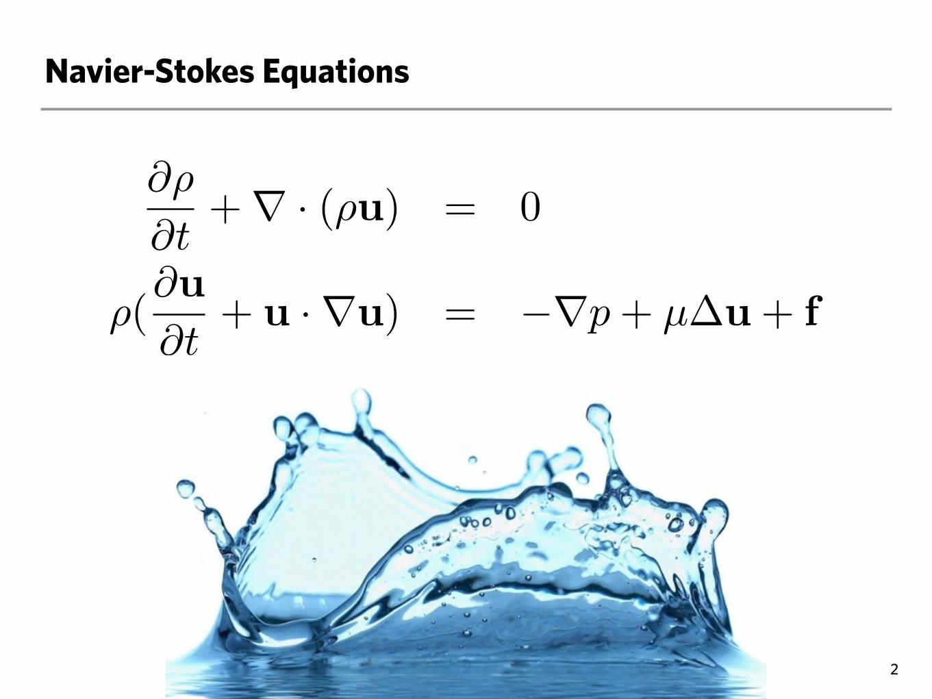
Navier-Stokes Equations
2
∂ρ
∂t+∇ · (ρu) = 0
ρ(∂u
∂t+ u ·∇u) = −∇p+ µ∆u+ f
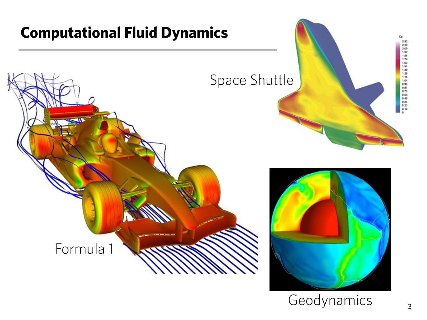
Computational Fluid Dynamics
3
Formula 1
Space Shuttle
Geodynamics

Computational Grid
4
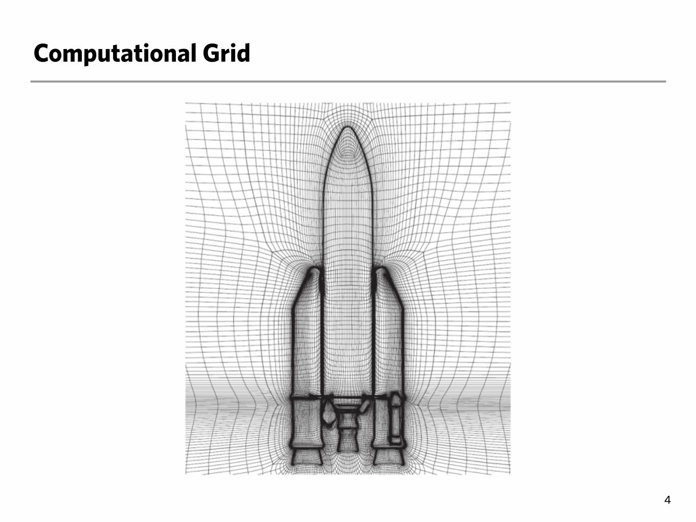
Computational Grid
4
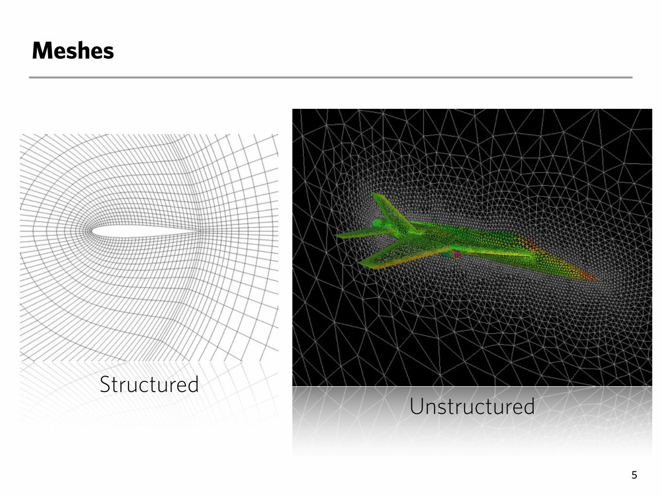
Meshes
5
StructuredUnstructured
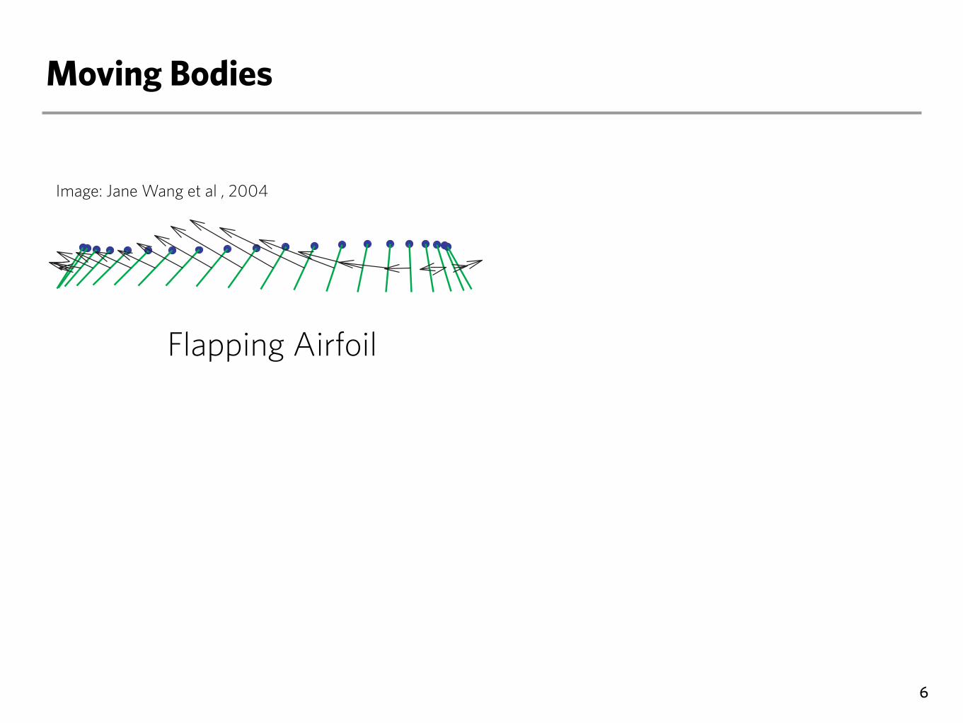
Moving Bodies
6
453Computation vs experiment in insect flight
The constants depend on the Reynolds number, details ofthe wing, etc. Unlike the Kutta–Joukowski lift, which is validat small values of ! and is proportional to sin!,Equations·12,13 and 14,15 are valid for all values of ! and
depend explicitly on 2!, rather than !. The 2! dependenceis consistent with the symmetry of a plate. Moreover, it isconsistent with the theoretical prediction of lift and drag of astalled wing:
CL = "sin(2!)/(4 + "sin!)·, (16)
CD = "sin2(!)/(4 + "sin!)·, (17)
which is derived assuming complete flow separation in thewake (von Karman and Burgers, 1963). The theoryunderpredicts the magnitude of the forces, but gives roughlythe right shape of the force curve. In addition, Equations·16,17make it apparent that the net force in the stalled case is normalto the wing, a prediction confirmed by our computations andexperiments (Figs·2–4). We refer to the forces, G#u2CL and
Fig.·2. Computational and experimental lift and drag coefficientsduring advanced rotation ($="/4; A0/c=2.8). (A) Lift (CL) and drag(CD) during the first four complete strokes. Red, experimentalmeasurements; blue, computations. The time is normalized with theflapping period. The force is normalized by the maxima of thecorresponding quasi-steady forces. (B) Experimental and (C)computational force vectors superimposed on wing positions, plottedat equal time intervals. The green line represents the wing chord;filled circles, the leading edge; arrows indicate force vectors on thewing. R, right; L, left.
0 0.5 1 1.5 2 2.5 3 3.5 4
0 0.5 1 1.5 2 2.5 3 3.5 4
–1 –0.50
0.51
1.52
C L –1.5
–1 –0.50
0.51
1.52
TimeC D
A
Stroke L
Stroke R
B
Stroke L
Stroke R
C
Fig.·3. Computational and experimental lift and drag coefficientsduring symmetrical rotation ($=0; A0/c=2.8). Details as in Fig.·2.
0 0.5 1 1.5 2 2.5 3 3.5 4
0 0.5 1 1.5 2 2.5 3 3.5 4
–1–0.50
0.51
1.52
C L
–1.5 –1
–0.50
0.51
1.52
Time
C D
A
Stroke L
Stroke R
B
Stroke L
Stroke R
C
Flapping Airfoil
Image: Jane Wang et al , 2004
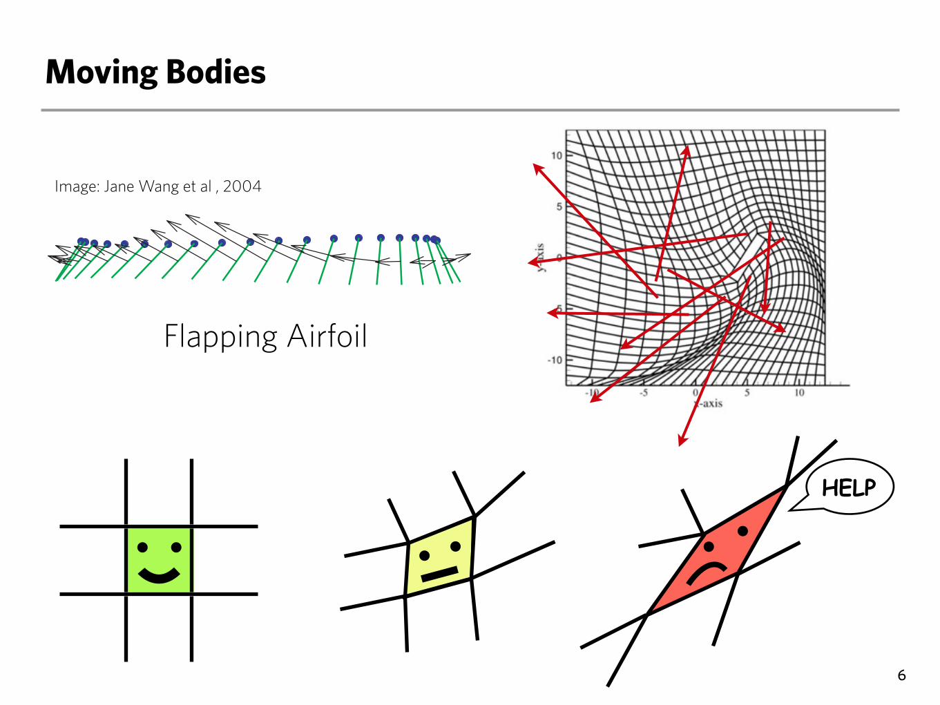
Moving Bodies
6
453Computation vs experiment in insect flight
The constants depend on the Reynolds number, details ofthe wing, etc. Unlike the Kutta–Joukowski lift, which is validat small values of ! and is proportional to sin!,Equations·12,13 and 14,15 are valid for all values of ! and
depend explicitly on 2!, rather than !. The 2! dependenceis consistent with the symmetry of a plate. Moreover, it isconsistent with the theoretical prediction of lift and drag of astalled wing:
CL = "sin(2!)/(4 + "sin!)·, (16)
CD = "sin2(!)/(4 + "sin!)·, (17)
which is derived assuming complete flow separation in thewake (von Karman and Burgers, 1963). The theoryunderpredicts the magnitude of the forces, but gives roughlythe right shape of the force curve. In addition, Equations·16,17make it apparent that the net force in the stalled case is normalto the wing, a prediction confirmed by our computations andexperiments (Figs·2–4). We refer to the forces, G#u2CL and
Fig.·2. Computational and experimental lift and drag coefficientsduring advanced rotation ($="/4; A0/c=2.8). (A) Lift (CL) and drag(CD) during the first four complete strokes. Red, experimentalmeasurements; blue, computations. The time is normalized with theflapping period. The force is normalized by the maxima of thecorresponding quasi-steady forces. (B) Experimental and (C)computational force vectors superimposed on wing positions, plottedat equal time intervals. The green line represents the wing chord;filled circles, the leading edge; arrows indicate force vectors on thewing. R, right; L, left.
0 0.5 1 1.5 2 2.5 3 3.5 4
0 0.5 1 1.5 2 2.5 3 3.5 4
–1 –0.50
0.51
1.52
C L –1.5
–1 –0.50
0.51
1.52
TimeC D
A
Stroke L
Stroke R
B
Stroke L
Stroke R
C
Fig.·3. Computational and experimental lift and drag coefficientsduring symmetrical rotation ($=0; A0/c=2.8). Details as in Fig.·2.
0 0.5 1 1.5 2 2.5 3 3.5 4
0 0.5 1 1.5 2 2.5 3 3.5 4
–1–0.50
0.51
1.52
C L
–1.5 –1
–0.50
0.51
1.52
Time
C D
A
Stroke L
Stroke R
B
Stroke L
Stroke R
C
Flapping Airfoil
HELP
Image: Jane Wang et al , 2004
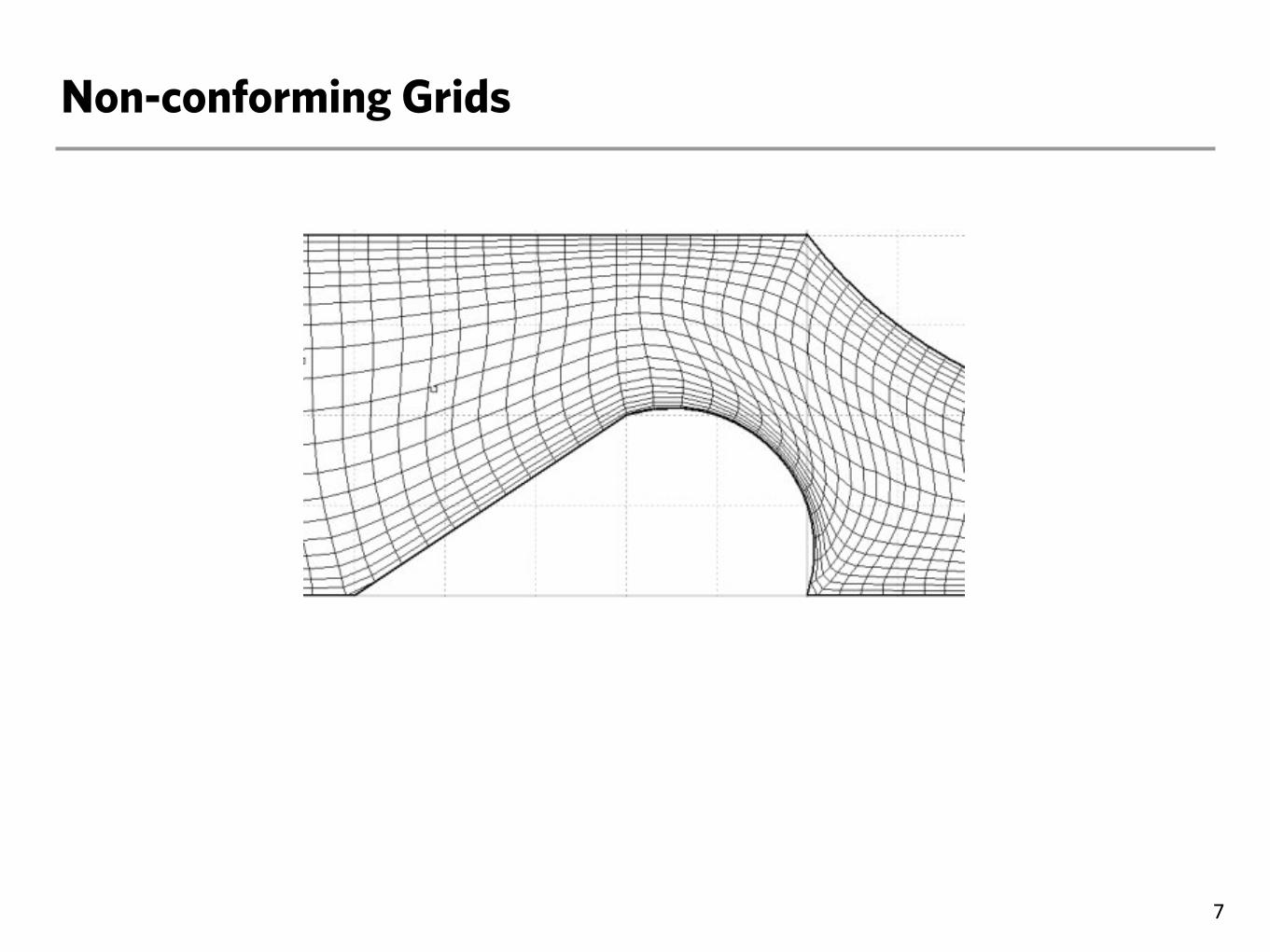
Non-conforming Grids
7
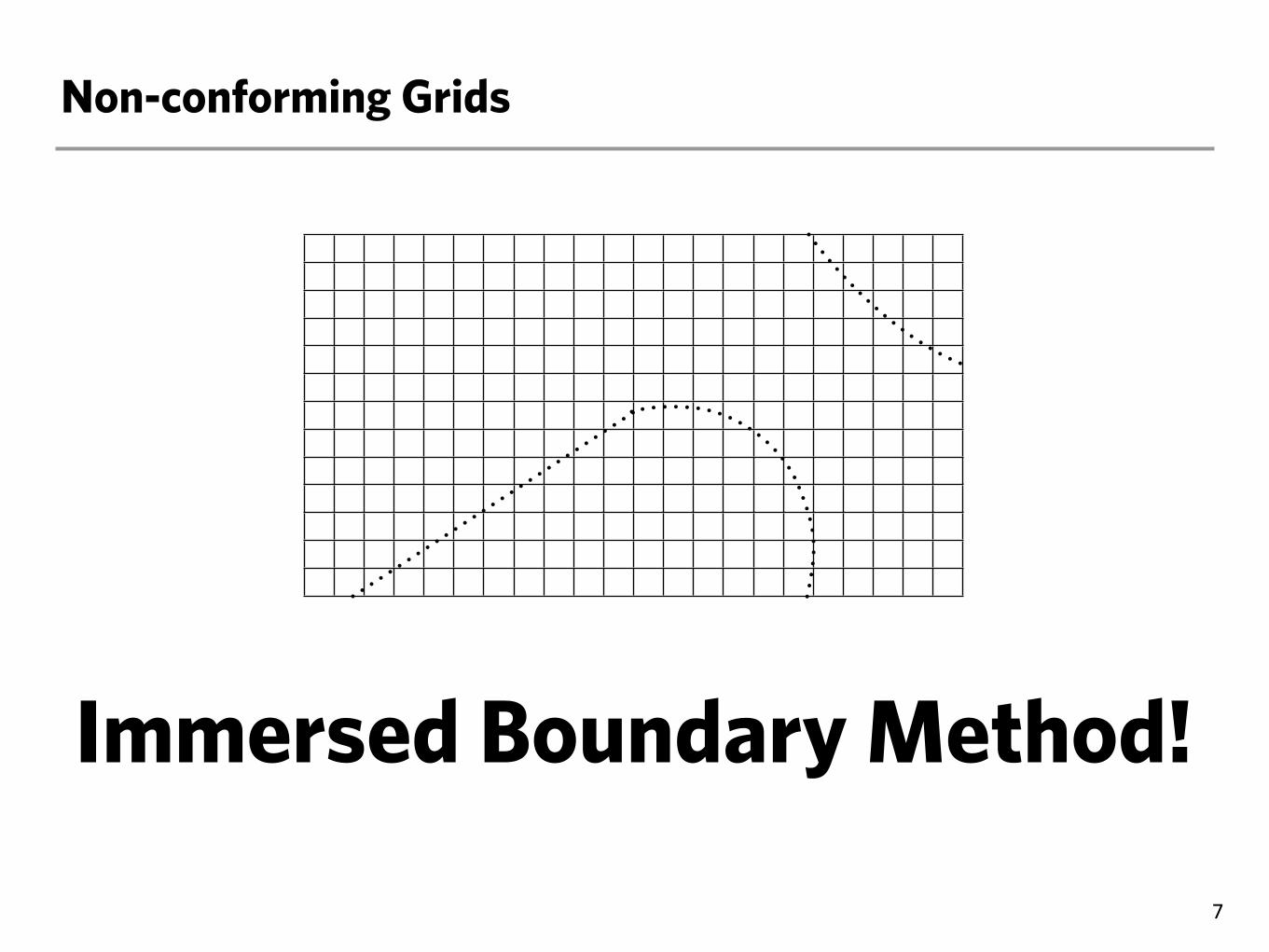
Non-conforming Grids
7
Immersed Boundary Method!
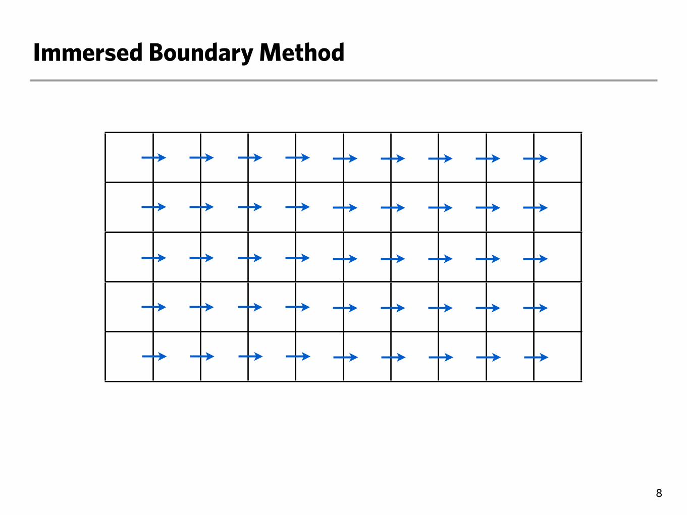
Immersed Boundary Method
8
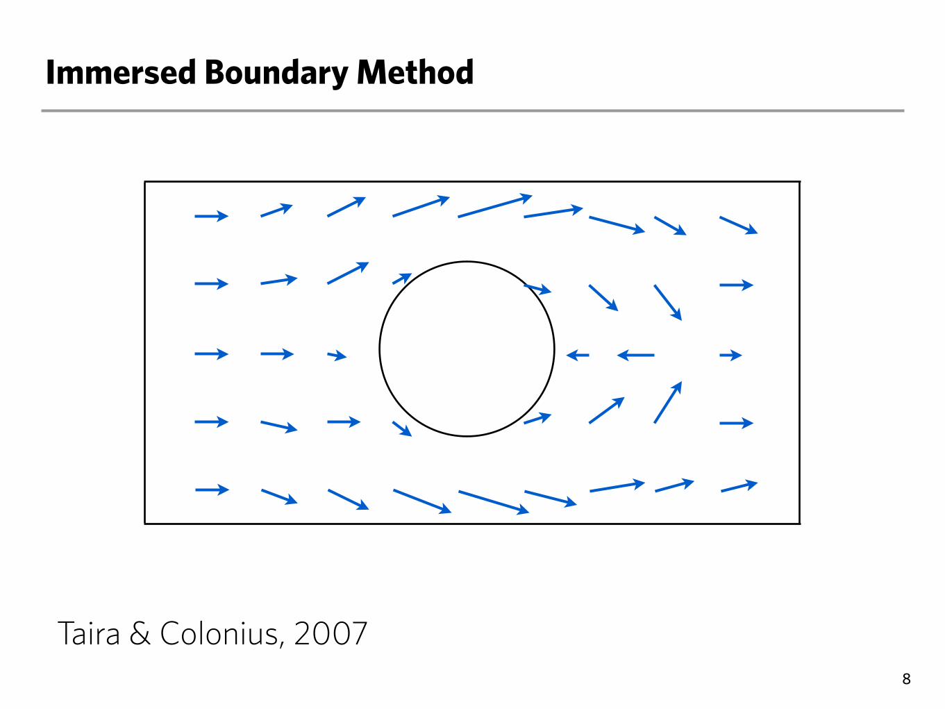
Immersed Boundary Method
8
Taira & Colonius, 2007
Immersed Boundary Method
9
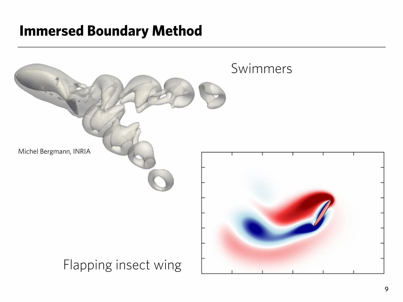
Flapping insect wing
Swimmers
Michel Bergmann, INRIA
Immersed Boundary Method
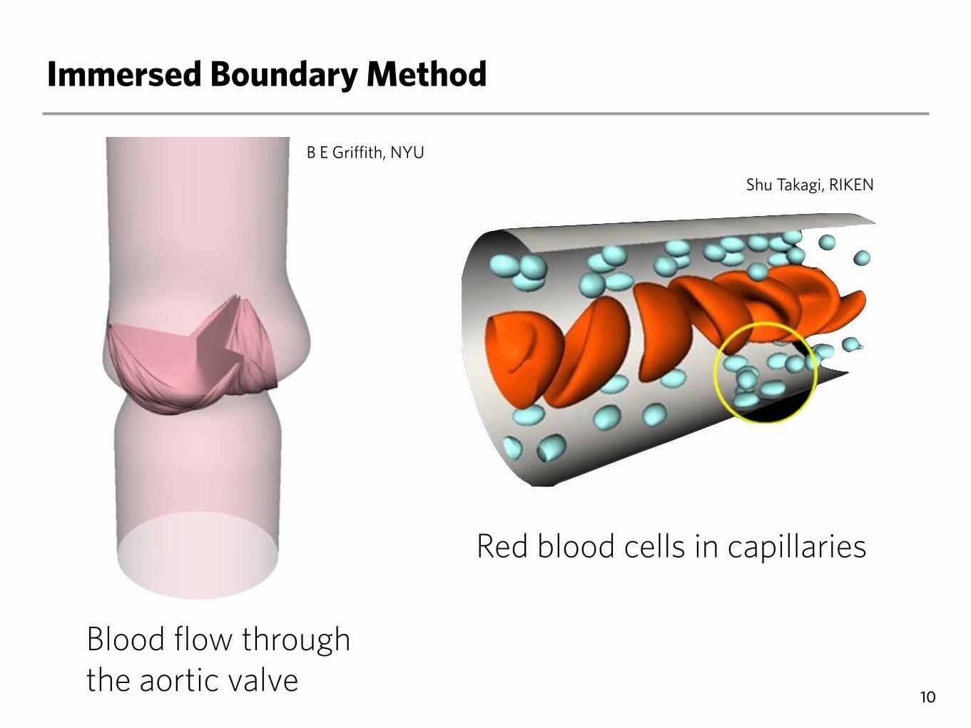
10
Blood flow through the aortic valve
Red blood cells in capillaries
B E Griffith, NYU
Shu Takagi, RIKEN
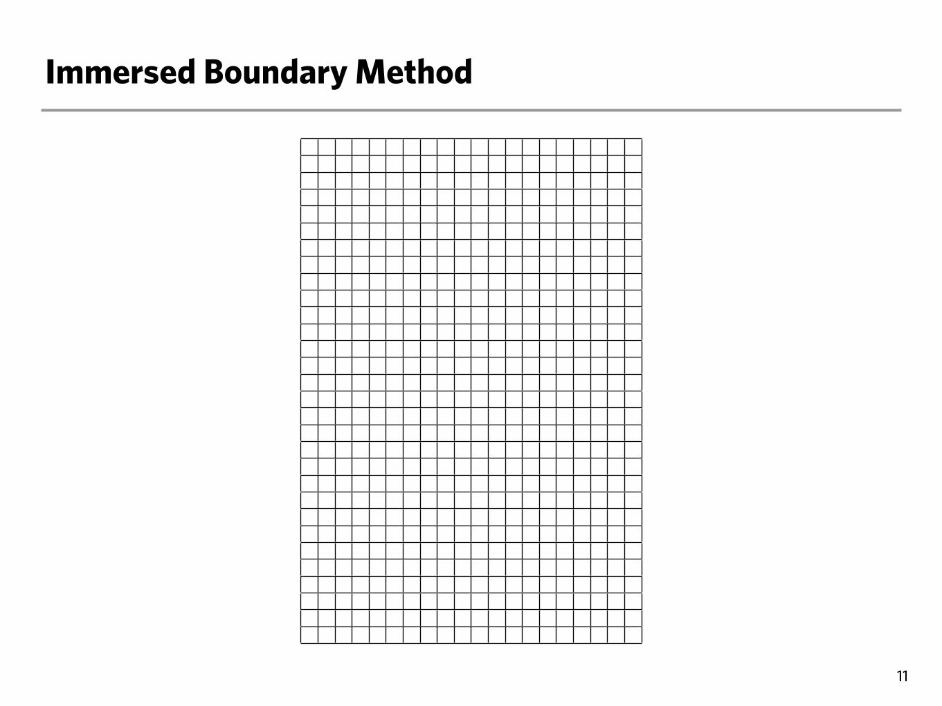
Immersed Boundary Method
11
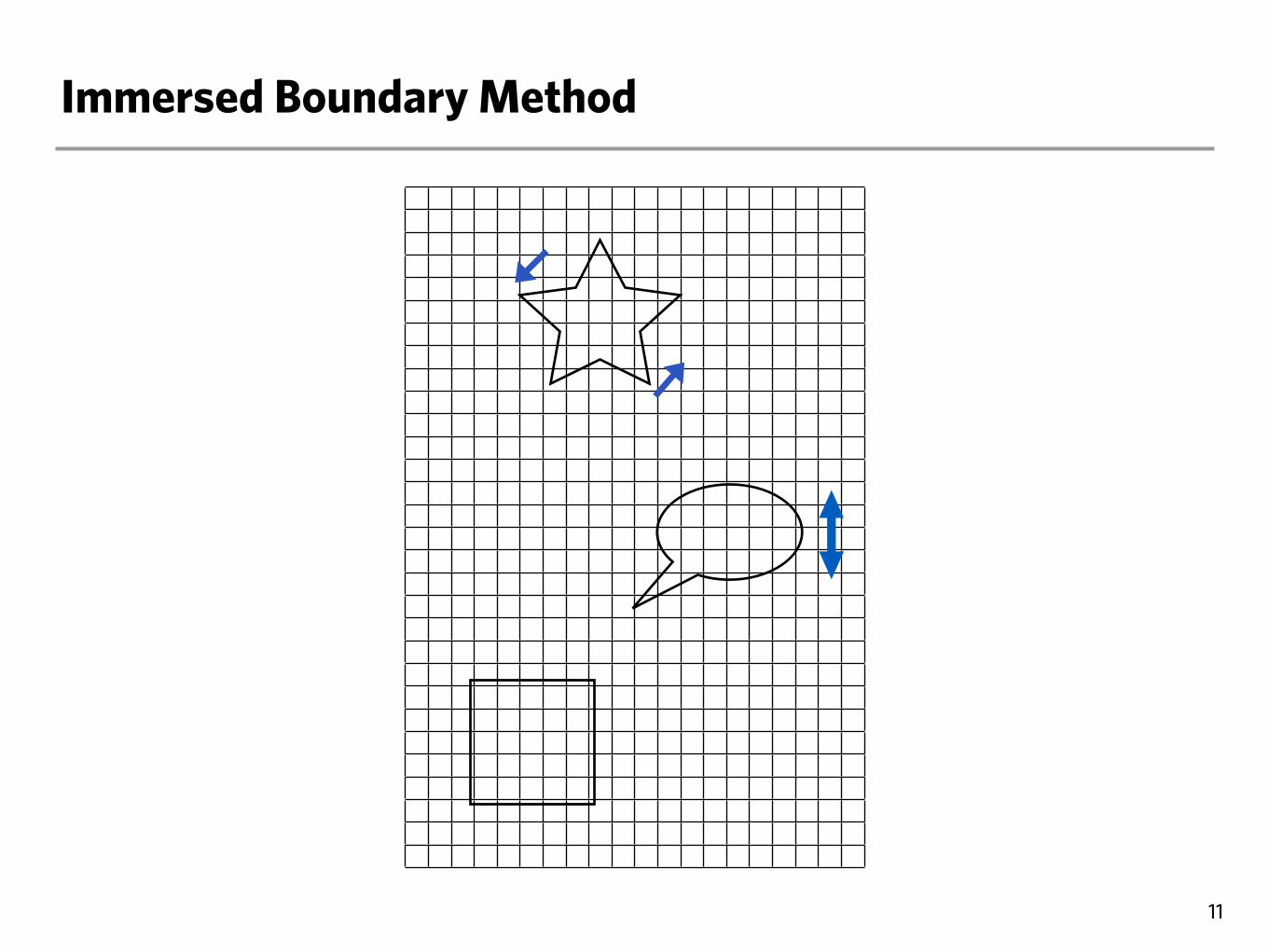
Immersed Boundary Method
11
Immersed Boundary Method
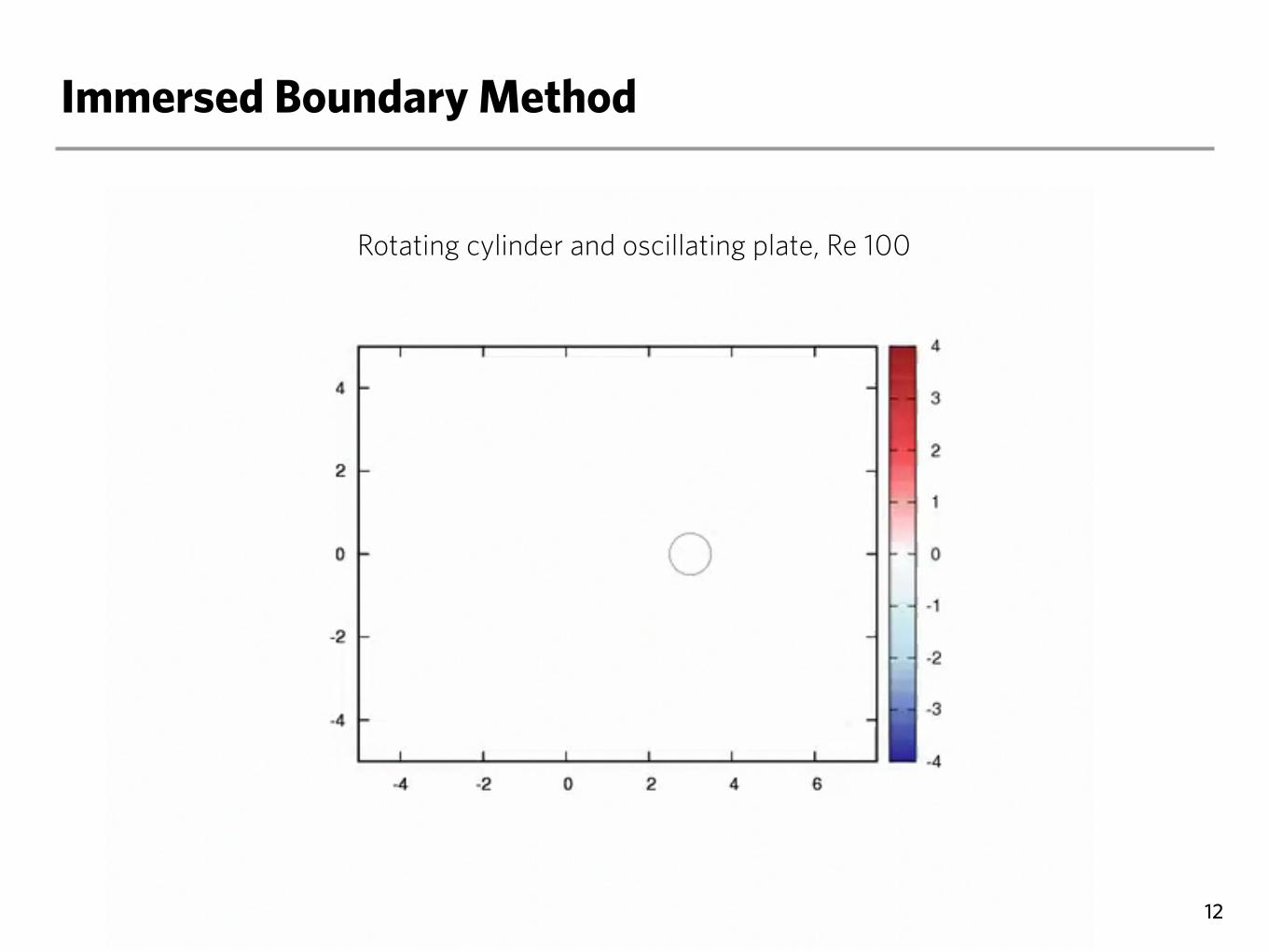
12
Rotating cylinder and oscillating plate, Re 100
GPU Acceleration
‣Pressure & force calculation - 90%
- Sparse Linear system
‣CUSP
- NVIDIA Research
‣Pressure solve (2-D)
- 9x faster (1 GPU vs 1 CPU core)
13
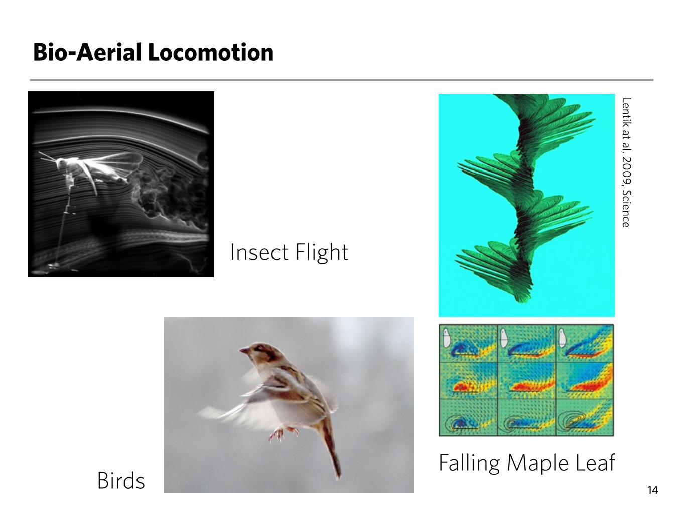
Bio-Aerial Locomotion
14
Insect Flight
BirdsFalling Maple Leaf
Lentik at al, 200
9, Science
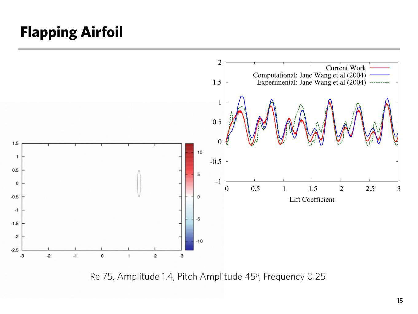
Flapping Airfoil
15
Re 75, Amplitude 1.4, Pitch Amplitude 45o, Frequency 0.25
-1
-0.5
0
0.5
1
1.5
2
0 0.5 1 1.5 2 2.5 3
Lift Coefficient
Current WorkComputational: Jane Wang et al (2004)
Experimental: Jane Wang et al (2004)
Flying Snakes
16
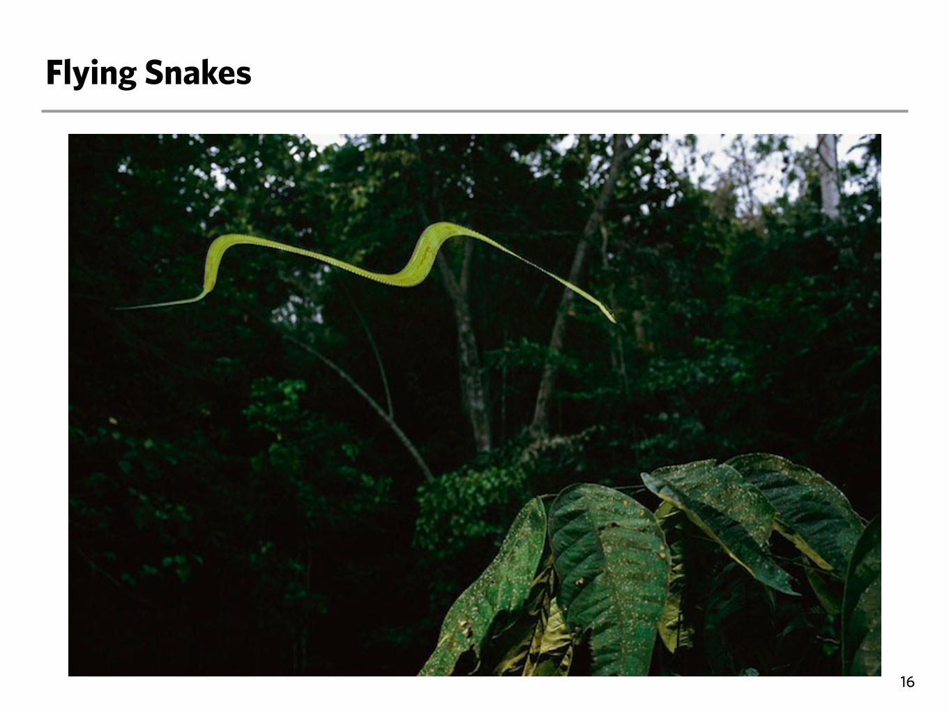
Flying Snakes
16
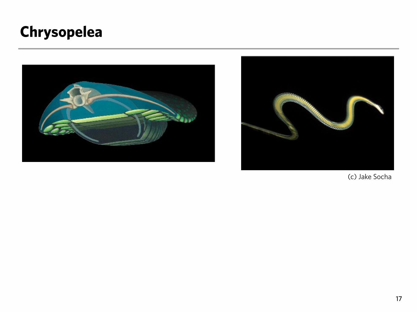
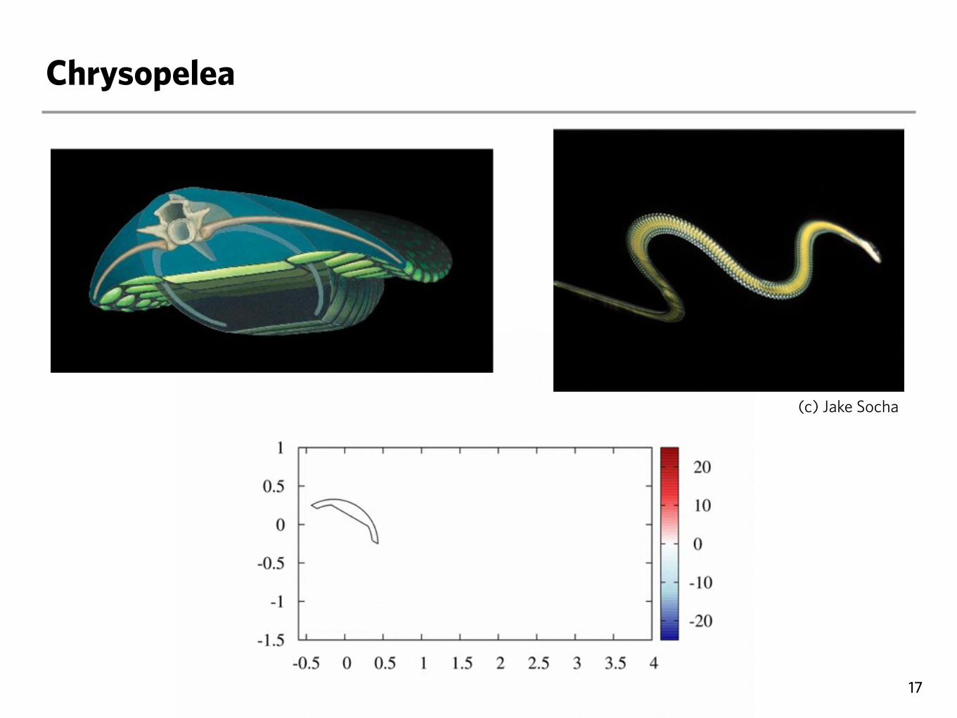
Chrysopelea
17
(c) Jake Socha
Chrysopelea
17
(c) Jake Socha
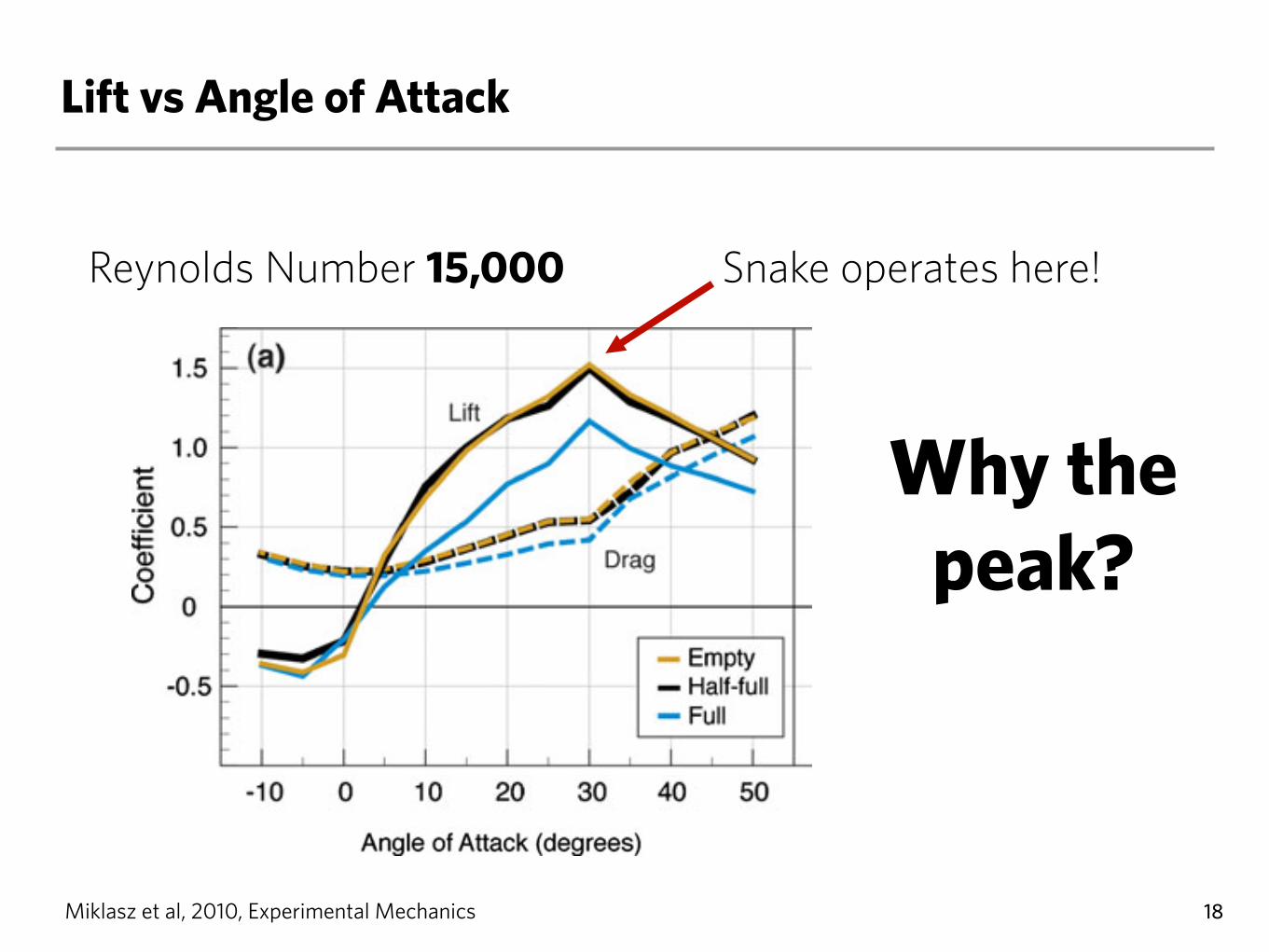
Lift vs Angle of Attack
18
Reynolds Number 15,000
Why the peak?
of the sharp model was similar to the half-full model withrounded edges [Figs. 3(b, e) and 4(b)] and polar plots forthese models were nearly identical [Fig. 4(b)].
Effects of a Dorsal (Top Surface) Protuberance
The ‘backbone’ model displayed much greater (and near-constant) drag and slightly lower lift [Fig. 3(b) and 4(b)]than the half-full model at each angle of attack between 0°and 30°. Both the backbone and the half-full model had thesame stall angle, 30°, and performed similarly at post-stallangles of attack. The maximum lift coefficient and maximalL/D ratio were smaller for the backbone model [Fig. 3(e)];L/D ratio peaked sharply over a very narrow range ofangles of attack (25° to 30°), unlike the 20° range (!=10°to 30°) of near-maximal L/D ratio in the base (half-full)model [Fig. 3(e)].
Tandem Models
We positioned models in tandem—upstream and down-stream—and measured aerodynamic forces on the down-stream model. When the downstream model was positioneddirectly behind the upstream model (stagger = 0; ‘draft-ing’), the drag coefficient of the downstream model (basedon free-stream airspeed) markedly decreased [Fig. 6(a)]relative to a solitary model at the same angle of attack(25°). The effect of drafting decreased as the gap increased.As the stagger increased (either in the positive or negativedirection), the drag coefficients of the downstream modelapproached those of a solitary model.
The lift coefficient of the downstream model exhibiteda more complicated relationship with relative position[Fig. 6(b)]. When the downstream model was directlybehind the upstream model (stagger = 0), the calculated
Fig. 3 Lift and drag character-istics vs. angle of attack for allmodels. Lift and drag coeffi-cients are plotted in (a–c), withlift represented by solid linesand drag represented by dashedlines; corresponding lift-to-drag(L/D) ratios are plotted in (d–f).(a, d) Comparisons of the emptyand full models to the half-fullmodel. (b, e) Comparisons ofthe sharp edge and backbonemodels to the half-full(= rounded edge) model. (c, f)Computational modeling results.For reference, the results for thehalf-full physical model are alsoshown (in gray)
Exp Mech (2010) 50:1335–1348 1341
Snake operates here!
Miklasz et al, 2010, Experimental Mechanics
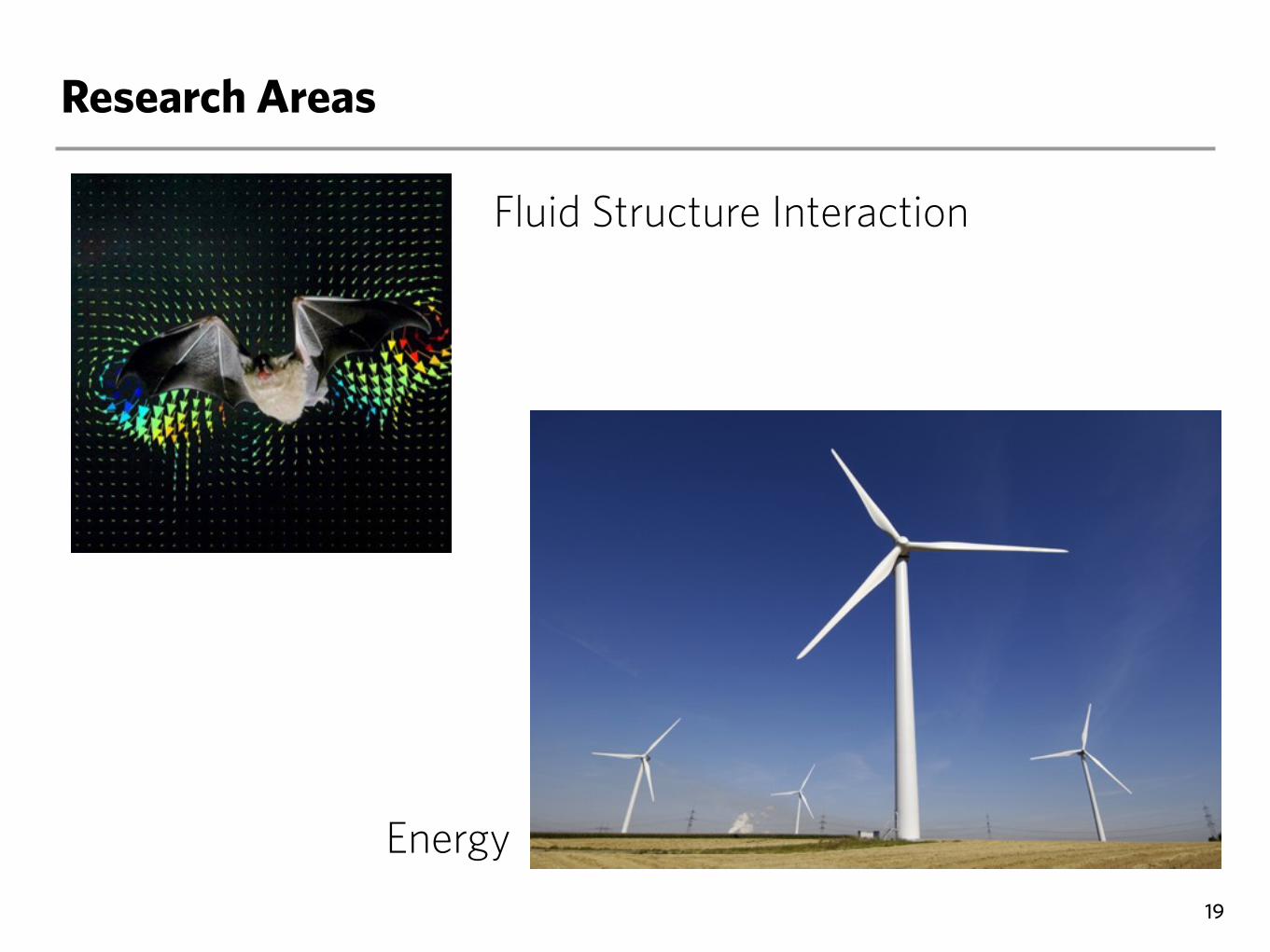
Research Areas
19
Fluid Structure Interaction
Energy
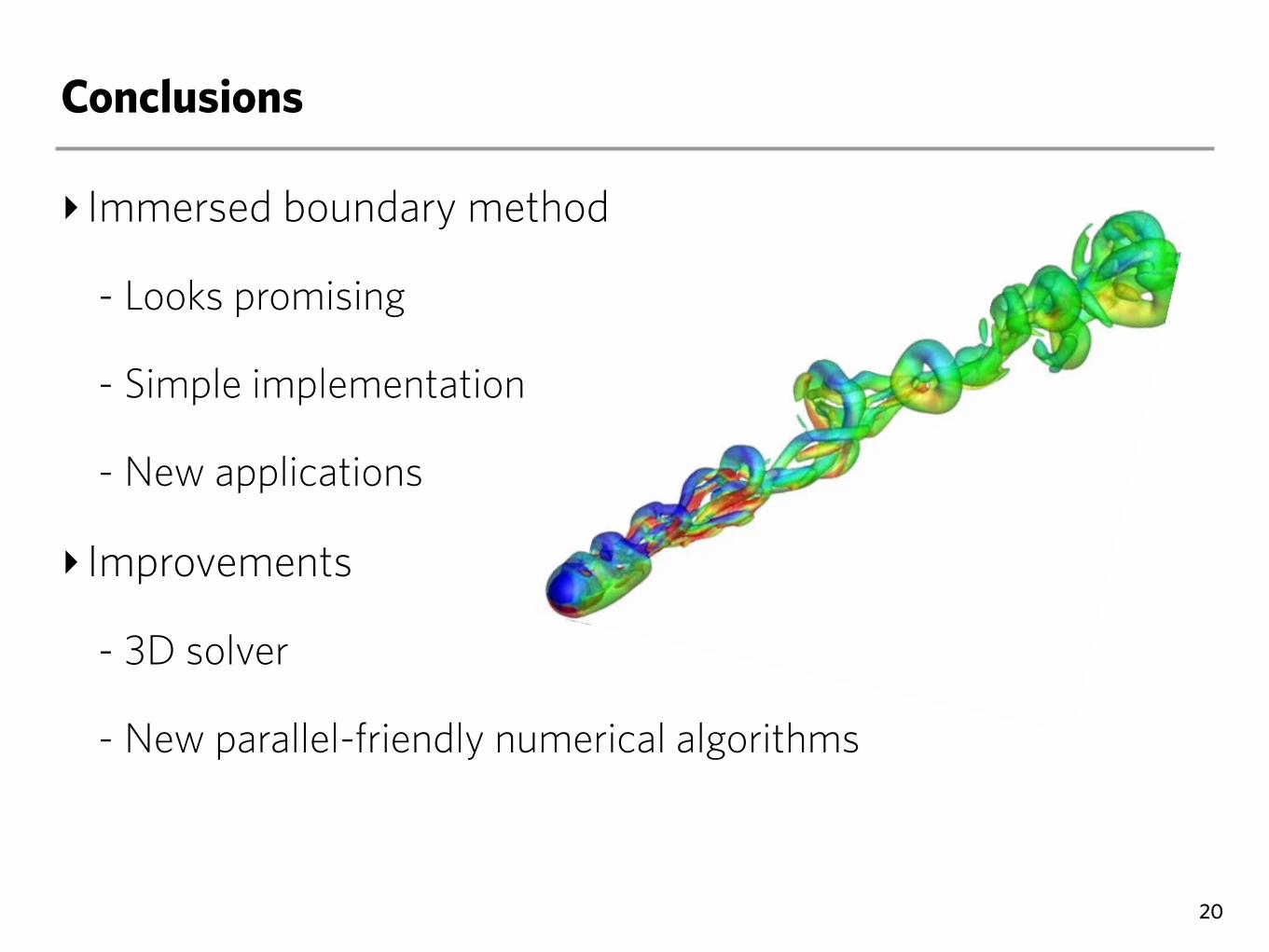
‣ Immersed boundary method
- Looks promising
- Simple implementation
- New applications
‣ Improvements
- 3D solver
- New parallel-friendly numerical algorithms
Conclusions
20


![Using GPUs for the Boundary Element Method · Boundary Element Method - Matrix Formulation ‣Apply for all boundary elements at 3 Γ j x = x i x 0 x 1 x 2 x 3 x = x i [A] {X } =[B](https://static.fdocument.org/doc/165x107/5fce676661601b3416186b00/using-gpus-for-the-boundary-element-method-boundary-element-method-matrix-formulation.jpg)