Paper presented at 48th Congress of the ERSA

How do Agglomeration Economies and Migration explain

the Change of Interregional Income Disparities?

Ryohei Nakamura¶ Department of Economics

Okayama University Japan

August, 2008

This paper investigates the causes of changing income disparities across regions by the extension of β convergence model. Increasing returns to scale in presence of agglomeration economies and of interregional population migration are included in the model. Agglomeration economies induce population in-migration due to higher productivity. The region experiencing population in-migration will decreases its productivity in a sense of neoclassical economic theory, i.e., the existence of decreasing returns to scale. At the same time, however, population in-migration has a possibility of enhancing agglomeration economies. If marginal effect of agglomeration economies is greater than decreasing marginal productivity of labour, then regional disparities may expand. This suggests a kind of the Verdoorn effect. Of course the differences of industrial composition across regions are another important cause of disparities. In this paper I present a consistent model which explains changing regional disparities and try to estimate the magnitudes of IRS by considering the existence of human capital. The model is a kind of the integration of Kaldorian model and endogenous growth model. The estimations are carried out by using Japanese regional data. Keywords: agglomeration economies, migration, income transfer, convergence/divergence,

regional income disparity ¶ E-mail ubbz0252@cc.okayama-u.ac.jp

1. Introduction

Convergence or divergence of per-capita income in an inter-regional economic system is an

essential topic to policy maker as well as scholars. In the long run, which implies more than

thirty years, interregional income disparities tend to show marked convergence. This is

confirmed in several countries including Japans by Barro and Sala-i-Martin (2004), and others.

However, the rate of decline in regional per-capita income disparities is not constant over the

period. Furthermore, in the course of economic progress we have often experienced

divergence of per-capita income across regions.

There are two competing theories which explain convergence/divergence of regional

disparities. The one is neoclassical growth theory including endogenous growth theory which

states convergence to the steady state solution. The other is cumulative growth theory which

suggests differential growth among regions. This is initially advocated by Kalor and

subsequently integrated to Verdoorn Law by Dixon and Thirlwall (1975).1

A number of papers have applied convergence model by Barro and Sala-i-Martin and also

structural convergence model proposed by Mankiw, Romer and Weil (1992) to regional

disparities in many countries.2 Although some earlier studies found regional convergence in

the long-run by applying β-convergence model, recent research is directed to explain

non-convergence trend or even divergence trend in regional disparities and to extend the

conditional convergence model. This is because of recent detection of increasing regional

disparities shown in several countries. For examples, Funke and Strulik (1999) found

increasing disparities of per-capita income since 1990 for Länder (states) in West Germany,

and Terrasi (1999) also verified divergence across Italian regions since 1975, and more

recently Longhi and Musolesi (2007) found the convergence process of the national

economies of the EU coexists with divergence process between regions in EU countries.

In order to overcome a shortcoming of the cross-sectional approach which neglects the

dynamic effects of growth and incorporate divergence effect into conditional convergence

model, several efforts have been done. Funke and Strulik propose an estimation model

1 Targetti and Foti (1999) estimated convergence equation and cumulative growth equation simultaneously for cross-country pooled data. 2 Crihfield and Panggabean (1995), Crihfield et al. (1955), Lall and Yilmaz (2001), Miller and Genc (2004) for US regions (states or metropolitan areas); Terrasi (1999) for Italian regions; de la Fuente (2002) for Spanish regions; Badinger et al (2004) for NUT 2 regions; Christopouls and Tsionas (2004) for Greece; Carluer and Gaulie (2005) for French regions; Armstrong (1955) for EU regions; and Henley (2003) for regions in the UK.

1

allowing for different convergence rate as well as different steady-states across regions and

estimate by panel data. 3 Hammond (2006) suggests divergence of regional disparities due to

the existence agglomeration economies created by knowledge spillovers and resulting

increasing returns to scale regional production function. Time variant model with a data

generating process is estimated by using time series of the US metropolitan data and shows

divergence between metropolitan and non-metropolitan incomes.

In a historical view the period when the nation is experiencing high economic growth,

income disparities across regions tend to increase, and then the relatively higher income

regions often accomplish higher growth rate of per-capita income than lower income regions

in such a period. The large metropolitan regions, which often exhibit relatively higher

income, are likely to generate endogenous growth and attract human capitals due to their

agglomeration economies. This cumulative causation implies the tradeoff between aggregate

efficiency and interregional equality.

When we observe decreasing regional disparities, economic disparities across regions

converge to a steady state level. On the contrary, in case of increasing or expanding regional

disparities, the economy is in transition to another steady state due to changing industrial

structure.

There are many sources which could change inter-regional income disparities. In a dynamic

context, migration is an important factor which can be the cause and/or result of regional

disparities as well as regional difference of technological progress. Many empirical studies

find agglomeration economies arising from population and industrial concentration will raise

regional productivity.

A regional income transfer by the national government is another important factor affecting

income disparities. Income transfer usually is implemented to poor regions in order to adjust

differences in local public finance. The total amount of transfer, in case of Japan, is

determined by the national tax revenue and political judgement.

In this paper I will focus on three main factors, which have been neglected in the

convergence model but important for changing regional income disparities, i.e.,

agglomeration, migration, and income transfers. Starting by the findings the contributions of

those factors to income disparities graphically, I provide the base of specification of the

3 Wang and Ge (2004) applied their model to Chinese provinces.

2

model. This is presented in the following section. The trends of regional per-capita income

disparities measured by the CV (Coefficient of Variation) are depicted with/without income

transfers and with excluding Tokyo. The graphical relationships between per-capita income

growth and agglomeration, income transfers, migration are also exhibited. Section 3 provide

neoclassical convergence model including agglomeration and regional migration.

Specification of the model presented in Section 3 is estimated and results are interpreted in

Section 4 by using Japanese regional data. Concluding remarks are given in Section 5.

2. Fact Findings on Regional Convergence/Divergence

In this section we will focus on the trend of regional disparities and examine some factors

which are seemed to be related to the change in regional income disparities. The candidates

for factors are agglomeration and migration, and income transfers. After graphically

examining such factors, I proceed to construct the model explaining regional

convergence/divergence.

2.1 Trend of Coefficient of Variation

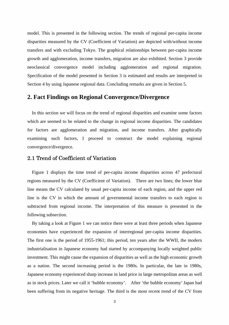
Figure 1 displays the time trend of per-capita income disparities across 47 prefectural

regions measured by the CV (Coefficient of Variation). There are two lines; the lower blue

line means the CV calculated by usual per-capita income of each region, and the upper red

line is the CV in which the amount of governmental income transfers to each region is

subtracted from regional income. The interpretation of this measure is presented in the

following subsection.

By taking a look at Figure 1 we can notice there were at least three periods when Japanese

economies have experienced the expansion of interregional per-capita income disparities.

The first one is the period of 1955-1961; this period, ten years after the WWII, the modern

industrialisation in Japanese economy had started by accompanying locally weighted public

investment. This might cause the expansion of disparities as well as the high economic growth

as a nation. The second increasing period is the 1980s. In particular, the late in 1980s,

Japanese economy experienced sharp increase in land price in large metropolitan areas as well

as in stock prices. Later we call it ‘bubble economy’. After ‘the bubble economy’ Japan had

been suffering from its negative heritage. The third is the most recent trend of the CV from

3

2000 to 2005.

Figure 1 Trend of per-capita income disparities measure by the CV: per-capita income with and without the governmental income transfer

'5557

5961

6365

6769

7173

7577

7981

8385

8789

9193

9597

'9901

0305

0.05

0.10

0.15

0.20

0.25

0.30

C.V.

After Transfer Before Transfer

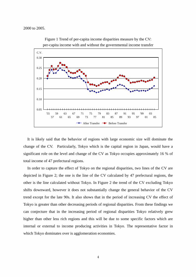
It is likely said that the behavior of regions with large economic size will dominate the

change of the CV. Particularly, Tokyo which is the capital region in Japan, would have a

significant role on the level and change of the CV as Tokyo occupies approximately 16 % of

total income of 47 prefectural regions.

In order to capture the effect of Tokyo on the regional disparities, two lines of the CV are

depicted in Figure 2; the one is the line of the CV calculated by 47 prefectural regions, the

other is the line calculated without Tokyo. In Figure 2 the trend of the CV excluding Tokyo

shifts downward, however it does not substantially change the general behavior of the CV

trend except for the late 90s. It also shows that in the period of increasing CV the effect of

Tokyo is greater than other decreasing periods of regional disparities. From these findings we

can conjecture that in the increasing period of regional disparities Tokyo relatively grew

higher than other less rich regions and this will be due to some specific factors which are

internal or external to income producing activities in Tokyo. The representative factor in

which Tokyo dominates over is agglomeration economies.

4

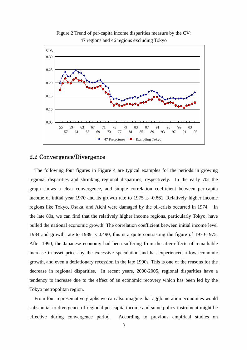
Figure 2 Trend of per-capita income disparities measure by the CV: 47 regions and 46 regions excluding Tokyo

'5557

5961

6365

6769

7173

7577

7981

8385

8789

9193

9597

'9901

0305

0.05

0.10

0.15

0.20

0.25

0.30

C.V.

47 Prefectures Excluding Tokyo

2.2 Convergence/Divergence

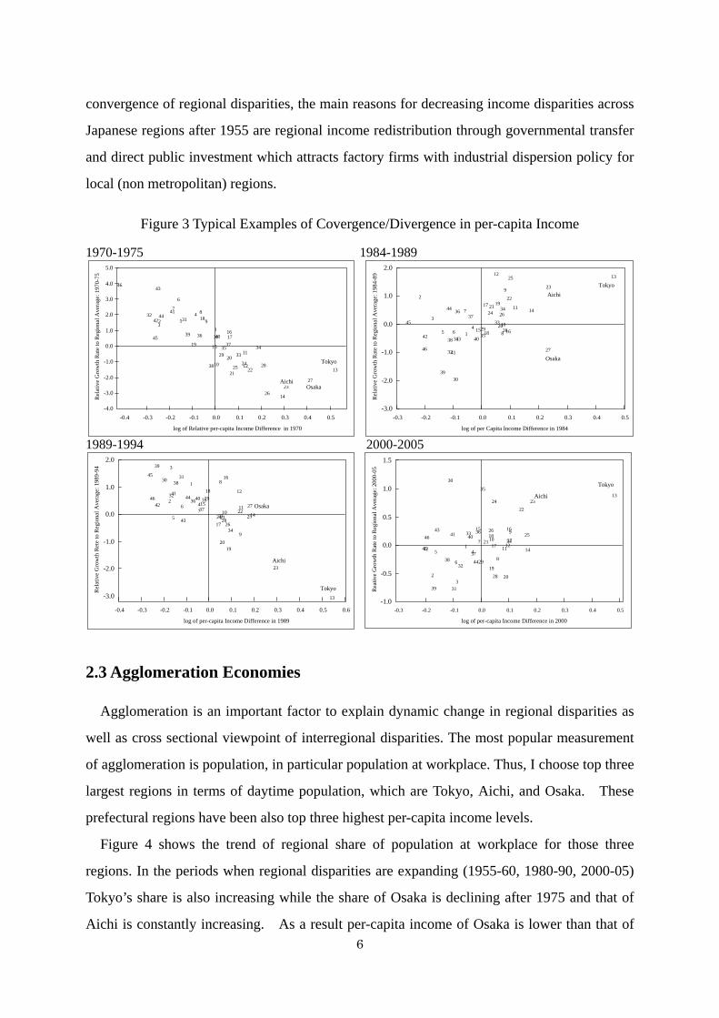
The following four figures in Figure 4 are typical examples for the periods in growing

regional disparities and shrinking regional disparities, respectively. In the early 70s the

graph shows a clear convergence, and simple correlation coefficient between per-capita

income of initial year 1970 and its growth rate to 1975 is -0.861. Relatively higher income

regions like Tokyo, Osaka, and Aichi were damaged by the oil-crisis occurred in 1974. In

the late 80s, we can find that the relatively higher income regions, particularly Tokyo, have

pulled the national economic growth. The correlation coefficient between initial income level

1984 and growth rate to 1989 is 0.490, this is a quite contrasting the figure of 1970-1975.

After 1990, the Japanese economy had been suffering from the after-effects of remarkable

increase in asset prices by the excessive speculation and has experienced a low economic

growth, and even a deflationary recession in the late 1990s. This is one of the reasons for the

decrease in regional disparities. In recent years, 2000-2005, regional disparities have a

tendency to increase due to the effect of an economic recovery which has been led by the

Tokyo metropolitan region.

From four representative graphs we can also imagine that agglomeration economies would

substantial to divergence of regional per-capita income and some policy instrument might be

effective during convergence period. According to previous empirical studies on 5

convergence of regional disparities, the main reasons for decreasing income disparities across

Japanese regions after 1955 are regional income redistribution through governmental transfer

and direct public investment which attracts factory firms with industrial dispersion policy for

local (non metropolitan) regions.

Figure 3 Typical Examples of Covergence/Divergence in per-capita Income

1970-1975 1984-1989

1989-1994 2000-2005

123

45

6

78

9

10

11

1213

14

15

1617

18

19

20

2122

23

2425

26

27

28

29

30

3132

333435

36

37

38

39 40

41

42

43

44

45

46

-0.4 -0.3 -0.2 -0.1 0.0 0.1 0.2 0.3 0.4 0.5

log of Relative per-capita Income Difference in 1970

-4.0

-3.0

-2.0

-1.0

0.0

1.0

2.0

3.0

4.0

5.0

Rel

ativ

e G

row

th R

ate

to R

egio

nal A

vera

ge: 1

970-

75

Tokyo

OsakaAichi

1

2

3

45 6

7

8

9

10

11

12 13

14

15 16

17

18

19

20

2122

23

24

25

26

27

2829

30

31

32

33

34

35

3637

38

39

40

41

42 43

44

45

46

-0.3 -0.2 -0.1 0.0 0.1 0.2 0.3 0.4 0.5

log of per Capita Income Difference in 1984

-3.0

-2.0

-1.0

0.0

1.0

2.0

Rel

ativ

e G

row

th R

ate

to R

egio

nal A

vera

ge: 1

984-

89

TokyoAichi

Osaka

1

2

3

4

5

67

8

9

1011

12

13

14

15

16

17

18

1920

2122

23

24 2526

27

28

29

30 31

32

33

34

3536

37

38

39

4041

42

43

44

45

46

-0.4 -0.3 -0.2 -0.1 0.0 0.1 0.2 0.3 0.4 0.5 0.6

log of per-capita Income Difference in 1989

-3.0

-2.0

-1.0

0.0

1.0

2.0

Rel

ativ

e G

row

th R

ete

to R

egio

nal A

vera

ge: 1

989-

94

Aichi

Osaka

Tokyo

1

23

45

6

7

8

910

1112

13

14

15 16

17

18

19

20

21

222324

2526

27

28

29

30

31

32

3334

35

36

3738

39

4041

42

43

44

45

46

-0.3 -0.2 -0.1 0.0 0.1 0.2 0.3 0.4 0.5

log of per-capita Income Difference in 2000

-1.0

-0.5

0.0

0.5

1.0

1.5

Rea

tive

Gro

wth

Rat

e to

Reg

iona

l Ave

rage

: 200

0-05

Tokyo

Aichi

2.3 Agglomeration Economies

Agglomeration is an important factor to explain dynamic change in regional disparities as

well as cross sectional viewpoint of interregional disparities. The most popular measurement

of agglomeration is population, in particular population at workplace. Thus, I choose top three

largest regions in terms of daytime population, which are Tokyo, Aichi, and Osaka. These

prefectural regions have been also top three highest per-capita income levels.

6

Figure 4 shows the trend of regional share of population at workplace for those three

regions. In the periods when regional disparities are expanding (1955-60, 1980-90, 2000-05)

Tokyo’s share is also increasing while the share of Osaka is declining after 1975 and that of

Aichi is constantly increasing. As a result per-capita income of Osaka is lower than that of

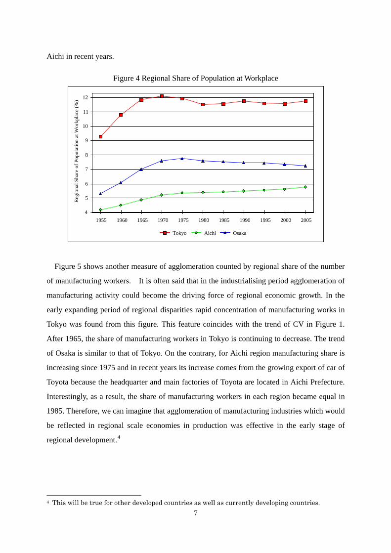
Aichi in recent years.

Figure 4 Regional Share of Population at Workplace

1955 1960 1965 1970 1975 1980 1985 1990 1995 2000 20054

5

6

7

8

9

10

11

12

Reg

iona

l Sha

re o

f Pop

ulat

ion

at W

orkp

lace

(%)

Tokyo Aichi Osaka

Figure 5 shows another measure of agglomeration counted by regional share of the number

of manufacturing workers. It is often said that in the industrialising period agglomeration of

manufacturing activity could become the driving force of regional economic growth. In the

early expanding period of regional disparities rapid concentration of manufacturing works in

Tokyo was found from this figure. This feature coincides with the trend of CV in Figure 1.

After 1965, the share of manufacturing workers in Tokyo is continuing to decrease. The trend

of Osaka is similar to that of Tokyo. On the contrary, for Aichi region manufacturing share is

increasing since 1975 and in recent years its increase comes from the growing export of car of

Toyota because the headquarter and main factories of Toyota are located in Aichi Prefecture.

Interestingly, as a result, the share of manufacturing workers in each region became equal in

1985. Therefore, we can imagine that agglomeration of manufacturing industries which would

be reflected in regional scale economies in production was effective in the early stage of

regional development.4

7

4 This will be true for other developed countries as well as currently developing countries.

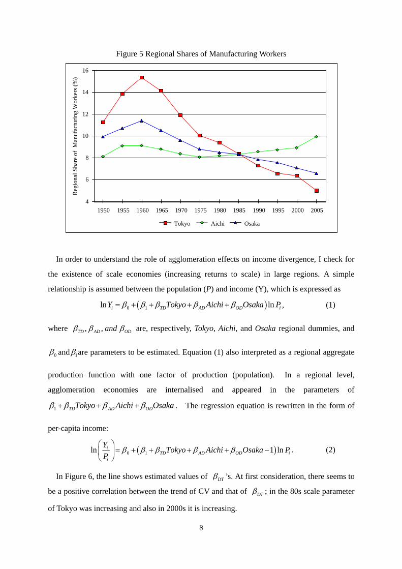
Figure 5 Regional Shares of Manufacturing Workers

1950 1955 1960 1965 1970 1975 1980 1985 1990 1995 2000 20054

6

8

10

12

14

16R

egio

nal S

hare

of

Man

ufac

turin

g W

orke

rs (%

)

Tokyo Aichi Osaka

In order to understand the role of agglomeration effects on income divergence, I check for

the existence of scale economies (increasing returns to scale) in large regions. A simple

relationship is assumed between the population (P) and income (Y), which is expressed as

, (1) ( )0 1ln lni TD AD ODY Tokyo Aichi Osaka Pβ β β β β= + + + + i

where , ,TD AD ODandβ β β are, respectively, Tokyo, Aichi, and Osaka regional dummies, and

0β and 1β are parameters to be estimated. Equation (1) also interpreted as a regional aggregate

production function with one factor of production (population). In a regional level,

agglomeration economies are internalised and appeared in the parameters of

1 TD ADTokyo Aichi ODOsakaβ β β β+ + + . The regression equation is rewritten in the form of

per-capita income:

( )0 1ln 1 lniTD AD OD i

i

Y Tokyo Aichi Osaka PP

β β β β β⎛ ⎞

= + + + + −⎜ ⎟⎝ ⎠

. (2)

In Figure 6, the line shows estimated values of DTβ ’s. At first consideration, there seems to

be a positive correlation between the trend of CV and that of DTβ ; in the 80s scale parameter

of Tokyo was increasing and also in 2000s it is increasing.

8

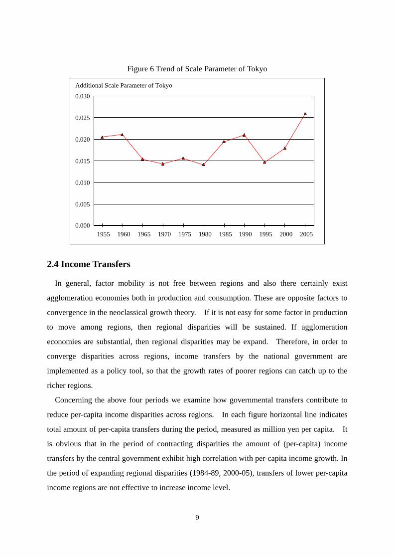
Figure 6 Trend of Scale Parameter of Tokyo

1955 1960 1965 1970 1975 1980 1985 1990 1995 2000 20050.000

0.005

0.010

0.015

0.020

0.025

0.030

Additional Scale Parameter of Tokyo

2.4 Income Transfers

In general, factor mobility is not free between regions and also there certainly exist

agglomeration economies both in production and consumption. These are opposite factors to

convergence in the neoclassical growth theory. If it is not easy for some factor in production

to move among regions, then regional disparities will be sustained. If agglomeration

economies are substantial, then regional disparities may be expand. Therefore, in order to

converge disparities across regions, income transfers by the national government are

implemented as a policy tool, so that the growth rates of poorer regions can catch up to the

richer regions.

Concerning the above four periods we examine how governmental transfers contribute to

reduce per-capita income disparities across regions. In each figure horizontal line indicates

total amount of per-capita transfers during the period, measured as million yen per capita. It

is obvious that in the period of contracting disparities the amount of (per-capita) income

transfers by the central government exhibit high correlation with per-capita income growth. In

the period of expanding regional disparities (1984-89, 2000-05), transfers of lower per-capita

income regions are not effective to increase income level.

9

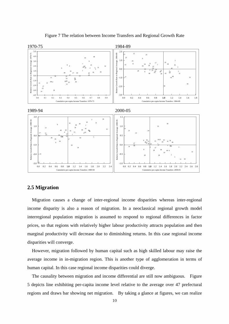
Figure 7 The relation between Income Transfers and Regional Growth Rate

1970-75 1984-89

12

3

45

6

78

9

10

11

1213

14

15

1617

18

19

20

2122

23

2425

26

27

28

29

30

3132

3334 35

36

37

38

3940

41

42

43

44

45

46

0.0 0.1 0.2 0.3 0.4 0.5 0.6 0.7 0.8 0.9

Cumulative per-capita Income Transfers: 1970-75

-4.0

-3.0

-2.0

-1.0

0.0

1.0

2.0

3.0

4.0

5.0

Rel

ativ

e G

row

th R

ate

to R

egio

nal A

vera

ge: 1

970-

75

1

2

3

456

7

8

9

10

11

1213

14

1516

17

18

19

20

21

22

23

24

25

26

27

28 29

30

31

32

33

34

35

3637

38

39

40

41

4243

44

45

46

0.0 0.2 0.4 0.6 0.8 1.0 1.2 1.4 1.6 1.81.0Cumulative per-capita Income Transfers: 1984-89

-3.0

-2.0

-1.0

0.0

1.0

2.0

Rel

ativ

e G

row

th R

ate

to R

egio

nal A

vera

ge: 1

984-

89

1989-94 2000-05

1

2

3

4

5

67

8

9

1011

12

13

14

15

16

17

18

1920

2122

23

242526

27

28

29

30 31

32

33

34

35 36

37

38

39

4041

42

43

44

45

46

0.0 0.2 0.4 0.6 0.8 1.0 1.2 1.4 1.6 1.8 2.0 2.2 2.41.0Cumulative per-capita Income Transfers: 1989-94

-3.0

-2.0

-1.0

0.0

1.0

2.0

Rel

ativ

e G

row

th R

ate

to R

egio

nal A

vera

ge: 1

989-

94

1

23

4 5

6

7

8

910

1112

13

14

1516

17

18

19

20

21

2223 24

2526

27

28

29

30

31

32

3334

35

36

3738

39

40 41

42

43

44

45

46

0.0 0.2 0.4 0.6 0.8 1.0 1.2 1.4 1.6 1.8 2.0 2.2 2.4 2.6 2.81.0Cumulative per-capita Income Transfers: 2000-05

-1.0

-0.5

0.0

0.5

1.0

1.5R

elat

ive

Gro

wth

Rat

e to

Reg

iona

l Ave

rage

: 200

0-05

2.5 Migration

Migration causes a change of inter-regional income disparities whereas inter-regional

income disparity is also a reason of migration. In a neoclassical regional growth model

interregional population migration is assumed to respond to regional differences in factor

prices, so that regions with relatively higher labour productivity attracts population and then

marginal productivity will decrease due to diminishing returns. In this case regional income

disparities will converge.

However, migration followed by human capital such as high skilled labour may raise the

average income in in-migration region. This is another type of agglomeration in terms of

human capital. In this case regional income disparities could diverge.

The causality between migration and income differential are still now ambiguous. Figure

5 depicts line exhibiting per-capita income level relative to the average over 47 prefectural

regions and draws bar showing net migration. By taking a glance at figures, we can realize 10

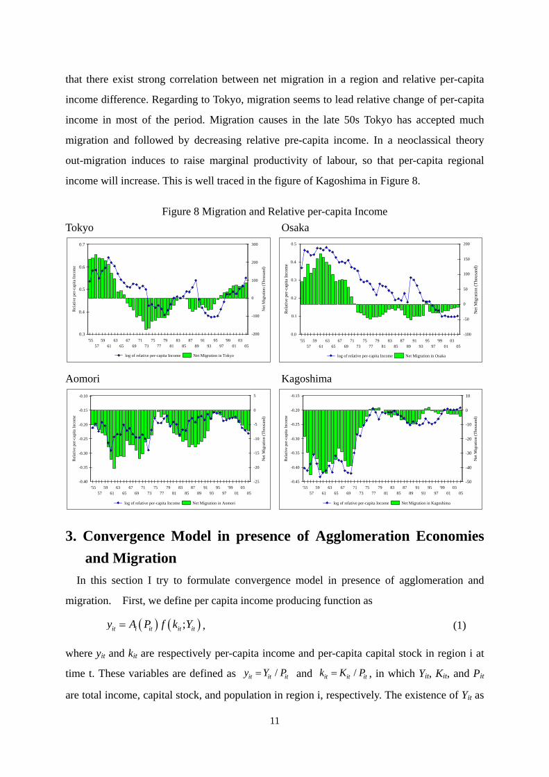
that there exist strong correlation between net migration in a region and relative per-capita

income difference. Regarding to Tokyo, migration seems to lead relative change of per-capita

income in most of the period. Migration causes in the late 50s Tokyo has accepted much

migration and followed by decreasing relative pre-capita income. In a neoclassical theory

out-migration induces to raise marginal productivity of labour, so that per-capita regional

income will increase. This is well traced in the figure of Kagoshima in Figure 8.

Figure 8 Migration and Relative per-capita Income Tokyo Osaka

'5557

5961

6365

6769

7173

7577

7981

8385

8789

9193

9597

'9901

0305

0.3

0.4

0.5

0.6

0.7

Rel

ativ

e pe

r-ca

pita

Inco

me

-200

-100

0

100

200

300

Net

Mig

ratio

n (T

hous

and)

log of relative per-capita Income Net Migration in Tokyo

'5557

5961

6365

6769

7173

7577

7981

8385

8789

9193

9597

'9901

0305

0.0

0.1

0.2

0.3

0.4

0.5

Rel

ativ

e pe

r-ca

pita

Inco

me

-100

-50

0

50

100

150

200

Net

Mig

ratio

n (T

hous

and)

log of relative per-capita Income Net Migration in Osaka

Aomori Kagoshima

'5557

5961

6365

6769

7173

7577

7981

8385

8789

9193

9597

'9901

0305

-0.40

-0.35

-0.30

-0.25

-0.20

-0.15

-0.10

Rel

ativ

e pe

r-ca

pita

Inco

me

-25

-20

-15

-10

-5

0

5

Net

Mig

ratio

n (T

hous

and)

log of relative per-capita Income Net Migration in Aomori

'5557

5961

6365

6769

7173

7577

7981

8385

8789

9193

9597

'9901

0305

-0.45

-0.40

-0.35

-0.30

-0.25

-0.20

-0.15

Rel

ativ

e pe

r-ca

pita

Inco

me

-50

-40

-30

-20

-10

0

10

Net

Mig

ratio

n (T

hous

and)

log of relative per-capita Income Net Migration in Kagoshima

3. Convergence Model in presence of Agglomeration Economies and Migration

In this section I try to formulate convergence model in presence of agglomeration and

migration. First, we define per capita income producing function as

( ) ( );it i it it ity A P f k Y= , (1)

where yit and kit are respectively per-capita income and per-capita capital stock in region i at

time t. These variables are defined as /it it ity Y P= and /it it itk K P= , in which Yit, Kit, and Pit

are total income, capital stock, and population in region i, respectively. The existence of Yit as

11

an argument in function f implies the possibility of increasing returns to scale due to

internalised agglomeration economies in a regional aggregated level. denotes Hicks

neutral shift factor of production.

( )i iA P

The change in capital stock, , is given by itK

, (2) it it itK I d K= − ⋅

where Iit is investment in region i and d is depreciation rate which is assumed to be constant

over the period and region. By dividing both side of equation (2) by Pit the change in per

capita capital, , is derived as itk

,it it

it it it K it it itit it

P Pk I d k s y d kP P

⎛ ⎞ ⎛ ⎞= − + = − +⎜ ⎟ ⎜ ⎟

⎝ ⎠ ⎝ ⎠, (3)

where sK,it is the proportion of investment in regional income.

In equation (3), unlike standard convergence model, population growth rate is variable over

the period. The reason for this is that there is high frequency of interregional migration

compared to international migration due to regional openness.5 Population change is divided

into natural change and social one. The separation of two factors is written as

. (4) it it it itP n P M= +

The migration rate is defined by it

itit

Mm =P , (5)

which is also dependent of regional characteristics such as relative per come level.

i

-capita in

Thus, m is rewritten as

( )/it it tm m y y= , (6)

where is the average value of yit over regions, and equation (6) is ( )/ /i it tty 0y y > .

At this point the causality between migration and per-capita income biguous. In

a neocla

dm d

level is am

ssical world, for regions experiencing positive net migration per-capita income will

decrease due to diminishing returns to scale with respect to labor. On the other hand, for

regions receiving in-migration of skilled-labor may increase per-capita income.

12

5 In their perspectives on regional economic growth, Niikamp and Poot (1998) formulate the endogenous growth model by considering labour migration.

Thus steady-state of capital intensity level is given by the equation:

( ) ( ) (, ,ln 0K it i it it itit it

it itit it

s A P f k Yd k k n d mdt k k

= = − + + =) . (7)

Let denote

(8a) ( ) ( ) ( ), /it Kit it it it it itG k s A P f k Y k=

and

( ) ( )it it itH k d n m k= + + , (8b)

where time subscript is added, and it ity k∝ is assumed. In equations (8a) and (8b), H(kit) is

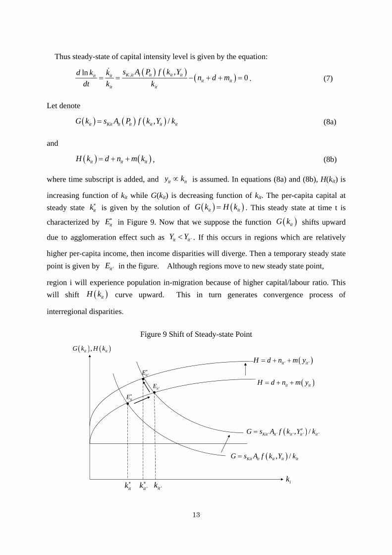
increasing function of kit while G(kit) is decreasing function of kit. The per-capita capital at steady state is given by the solution of itk∗ ( ) ( )it itG k H k= . This steady state at time t is

characterized by in Figure 9. Now that we suppose the function shifts upward

due to agglomeration effect such as

itE∗ ( )itG k

'Yit itY < . If this occurs in regions which are relatively

higher per-capita income, then income disparities will diverge. Then a temporary steady state point is given by ' in the figure. Although regions move to new steady state point, itE

region i will experience population in-migration because of higher capital/labour ratio. This will shift ( )itH k curve upward. This in turn generates convergence process of

interregional disparities.

Figure 9 Shift of Steady-state Point

ikitk∗

( )' ' ' ' ', /Kit it it it itG s A f k Y k′=

( )it itH d n m y= + +

( ), /Kit it it it itG s A f k Y k=

'itk

( ) ( ),it itG k H k

( )' 'it itH d n m y= + +

itE∗

'itE

'itE∗

'itk ∗

13

Even if region i is not on the steady state path at time t, per-capita income of region i

approaches to the steady state under the conditions that exhibits negative slope and

does positive slope, with respect to ki , respectively. Since there is no reason that at time t

region i is on the steady-state path, the approaching to steady-state in terms of per-capita

income of region i is usually described by the partial adjustment equation as

itE∗ G

H

'ln ln ln lnit it it it

t t t t

y y yb yy y y y

∗⎛ ⎞− = −⎜

⎝ ⎠⎟ , (9)

where yit is per-capita income at period t in region i and ity∗ is its equilibrium solution at t. The

convergence equation which has been tested in many regiona and countries is derived from

this equation and the coefficient which is derived from solving difference-equation (9), as a

function of , denotes a speed of convergence. The right hand side of equation is

approximately equal to the growth rate of per-capita income in region i measured by the

deviation from the regional average. The convergence equation is

b

'ln lnit it

it t

y yay

β= +y . (10)

In convergence model β is assumed to be constant over the period. If β takes the negative

value, then regions deviating from the steady state in terms of per-capita income would

converge. However, regions with relatively higher per-capita income may grow faster than the

regions with relatively lower per-capita income due to agglomeration effects, and furthermore

higher income level will attract human capital from lower regions, which in turn induces

in-migration. Therefore, we cannot deny the non-negativity of β as well as its constancy

over the period.6

As shown in Figure 9, the transition of steady-state may occur during [t, t’]. In this case

parameter β will depend upon the difference of two equilibrium levels of per-capita income,

'ln lneit ity y∗− (superscript ‘e’ means expectation of equilibrium value at current period), and

migration rate explaining the shift of equation (8b). Therefore, constant parameter β can be

14

6 There are some papers which try to specify and estimate the changing convergence parameters in order to capture regional divergence.

written by the functional form like

',( , ')ln ,

eit

i t tit

y my

β β ∗

⎛ ⎞= ⎜

⎝ ⎠⎟ . (11)

In equation (11), it is expected that the effect of migration on β will be positive because

migration promotes to converge inter-regional per-capita income disparities by diminishing

returns to labour in neoclassical model. On the other hand, the speed of convergence to new

steady-state will decline due to the additional change of steady-state or high expectation of

new steady-state may causes divergence.

4. Specification of the Model

First, I will define the Cobb-Douglas production function for firms with agglomeration

economies. In a specification of a firm-level production function agglomeration economies

are external to individual firms, and then the production function is expressed as 1

0ij i i iy P Y k lη γ α αα −= , (12)

and

, ,i ii i i

i i

Y Ky k lE E

= = = i

i

LE

,

where is the number of firms, is produced income per firm, is capital stock per

firm, and is labour which is measured as employees per firm. is the total produced

income in region i, and external to individual firms.

iE ijy ijk

iYijl

In aggregating into a regional level the production function is rewritten as

( )

1

1i i i i i i

i i i i i i

Y A P K L Y

A P K P Y

η α α γ

αη α κ

−

−

=

= γ, (13)

where labour is assumed to be the constant ratio of population, iκ .

Rewriting Equation (13) in terms of per-capita income gives the estimation form as 1/(1 ) (1 ) / (1 ) (1 )/ (1 ) / (1 )

i i i i iY A P Kγ α γ α η γ α γκ− − − − + − −= , (14)

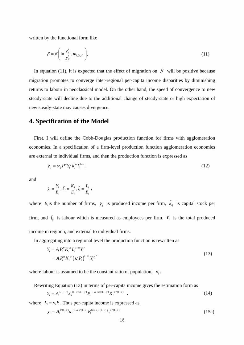
where ii iL Pκ= . Thus per-capita income is expressed as 1/(1 ) (1 ) / (1 ) ( ) / (1 ) / (1 )P ki i i i iy A γ α γ η γ γ α γκ− − − + − − = (15a)

15

or 1

i i i i i iy A k Y Pα α γ ηκ −= , (15b)

where

Equation (15a) indicates the industry-level production function in which agglomeration

ies presented by regional aggregate income are internalised. Thus, the regional

ag

/ , /i i i i ik K P and y Y P= = .i

econom

gregate production function exhibits increasing to returns to scale when γ is positive,

even given constant returns to scale at the firm level.

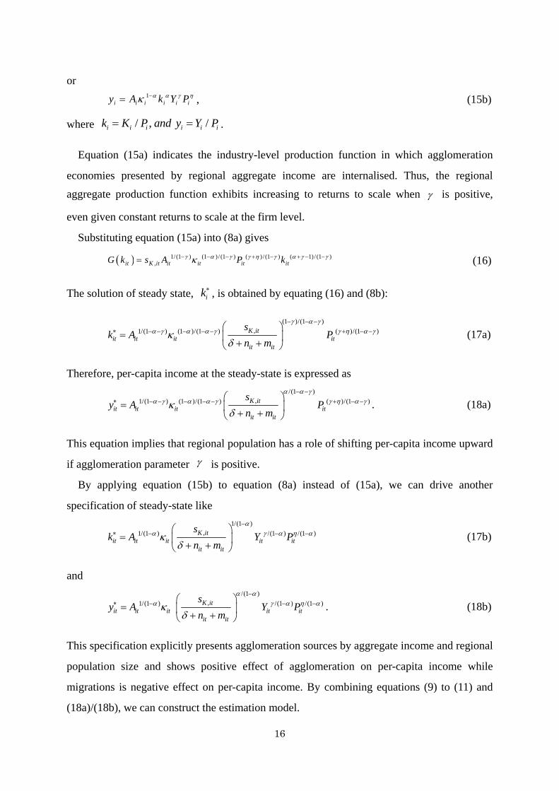
Substituting equation (15a) into (8a) gives

( ) 1/ (1 ) (1 ) / (1 ) ( ) / (1 ) ( 1,it K it it it it itG k s A P k ) / (1 )γ α γ γ η γ α γκ− − − + − + −= γ− (16)

The solution of steady state, , is obtained by equating (16) and (8b): ik∗

(1 )/(1 ),1/(1 ) (1 )/( ) ( )/(1 )K it

it it it itit it

k A Pn m

1 s γ α γα γ α γ γ η α γκ

δ∗ − − − − + − −= ⎜ ⎟+ +⎝ ⎠

α− − −

− ⎛ ⎞ (17a)

herefore, per-capita income at the steady-state is expressed as

T/(1 )

,1/(1 ) (1 )/(1 ) ( )/(1 )K itit it it it

it itn ms

y A Pα α γ

α γ α α γ γ η α γκ− −

∗ − − − − − + − −⎛ ⎞= ⎜ ⎟ . (18a)

This equation implies that regional population has a role of shifting

if agglomeration parameter

δ + +⎝ ⎠

per-capita income upward γ is positive.

By applying equation (15b) to equation (8a) instead of (15a), we can drive another

specification of steady-state like

1/(1 )

,1/(1 ) /(1 ) /(1 )K it

it

sk A Y P

n m

α

it it it it itit

α γ α η ακδ

−∗ − − −⎛ ⎞= ⎜ ⎟+ +⎝

(17b) ⎠

nd a/(1 )

,1/(1 ) /(1 ) /(1 )K itit it it it it

it it

sy A Y P

n m

α αα γ α η ακ

δ

−∗ − −⎛ ⎞= ⎜ ⎟+ +⎝ ⎠

− . (18b)

This specification explicitly presents agglomeration sour

population size and shows positive effect of agglomeration on per-capita income while

ces by aggregate income and regional

migrations is negative effect on per-capita income. By combining equations (9) to (11) and

(18a)/(18b), we can construct the estimation model.

16

5. Estimation of the Model

5.1 Data

n, the most relevant Japanese regional counterpart of

gions is ‘prefectures’ in Japan. There are 47 prefectures including the Tokyo

ion and job occupation by region are from

Census of Population which is issued by each five

lled grant-in-aid from tax revenue; it is redistributed to local

municipalities (cities, to

eter function

With regard to regional classificatio

NUTS 2 re

Metropolis, which has 23 special wards, similar to inner London. Each prefecture is a local

government and has its own governor. The average area over the 47 prefectural regions is

approximately 7,930 km2, which is slightly larger than the average of 36 NUTS 2 regions in

the UK, which is 6,773 km2.

The data on income are from the Cabinet Office in Japan, ‘Annual Report on Prefectural

Income’ (various issues) and data on populat

year. In terms of statistical availability we

can use data on the Regional System of Accounts (Annual Report on Prefectural Income) as

for back as 1955.

The data on income transfers by the national government are also available since 1955.

Income transfer is ca

wns, villages, and prefectures) for which the amount of local financial

demand exceeds local tax revenue.

5.2 Estimation Model

In specifying convergence param β we add two variables which will be

pita income level by the investigation of graphs in section 2. The significant to explain per-ca

one is the income transfers conducted by the national government, which would help to

converge income disparities across regions, denoted by itS . The other is the number of

skilled workers which acts as human capital in a regional economy. Migration brings skilled

labour force which will be affect positively per-capita in e growth. Hence, the varying

parameter model of convergence parameter

com

β is written as

' '' '

t t0 1ln ln

e t tit it it it

P H H Sit it itit

P H M Sb b b b bββ⎛ ⎞

= + + + +⎜ ⎟⎝ ⎠H P PP ∑ ∑ . (19)

The estimation equation is obtained by substituting equation (19) into equation (10) as

17

' '

lnt

it itS yb+ ∑ , (20)

' ' '0 1ln ln ln

tit it it it

P H H St tit it it it it t

y P H Ma b b b by P H P P yβ

⎛ ⎞⎛ ⎞= + + + +⎜ ⎟⎜ ⎟⎜ ⎟⎝ ⎠⎝ ⎠

∑

where the expected signs of parameters are 0bβ < , 0Pb > , 0 0Hb < ,

i

e regional disparities, i.e.,

1Hb >

es have negative im

0 , and 0Sb > .

The positive sign of parameter means agglom

convergence. Migration in general tends 0 0Hb

Pb eration econom

g

pact on

to conver <

because of diminishing returns to labour, while parameter b may be positive as human

capital represented by skilled labour can be brought with population in-migration t

contributes to increase regional per-capita income. Finally, the sign of income transfers is

expected to be positive since the role of transfers is contract to regional disparities

5.3 Estimation Results

In the estimation some variables have endogenous characteristics which

H1

and i

means a

m, so that we use the two-stage least squares method with

instrum

By considering figures 1 to 5 I select five typical sub-periods which shows increasing in

terms of the CV; 1955-1960, 1984-1989, 2000-2005, and decreasing in the CV; 1970-1975,

is that the purpose of this paper is to

investigate how agglom

correlation to the error ter

ental variables in order to deal this endogeneity problem. The candidates of

instruments are lagged dependent variables.

1989-1994. The reason I do not use the whole period

eration and migration economies affect change in regional disparities.

If we try to estimate agglomeration effect on regional disparities in the long-run, it will be

failed to capture it correctly.

The estimations are carried out by two types of specification of agglomeration economies

in addition to simple β -convergence model. The one is equation (19) in which the parameter

of regional population change reflect agglomeration effect, and the other is regional aggregate

incom

parameter of change in regional aggregate income,

e is adopted as the agglomeration variable instead of regional population, in which the

( )'it it

coefficient in Kaldorian cumulative growth model.

ln /Y Y , implies so-called Verdoorn

18

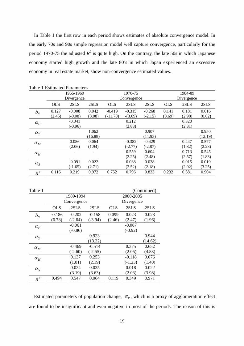
In Table 1 the first row in each period shows estim solute convergence model. In

period 1970-75 the adjusted R2 is quite high. On the contrary

ates of ab

the early 70s and 90s simple regression model well capture convergence, particularly for the

, the late 50s in which Japanese

econom

1984-89 Divergence

y started high growth and the late 80’s in which Japan experienced an excessive

economy in real estate market, show non-convergence estimated values.

Table 1 Estimated Parameters 1955-1960

Divergence 1970-75

Convergence OLS 2SLS 2SLS OLS 2SLS 2SLS OLS 2SLS 2SLS

bβ 0.127 -0.008 0.04(2.45)

2 (3.08)

-0.419 (-11.70)

-0.315 -0.268 (-2.15)

0.141 (3.69)

0.181 0.016 (0.62) (-0.08) -(3.69) (2.98)

Pα -0.041

(-0.96) 0.212 (2.88)

0.320 (2.31)

Yα 1.062 (16.88)

0.907 (11.93)

0.950 (12.19)

Mα 0.086 (2.06)

0.064 (1.94) (-2.87) (2.23)

-0.382 (-2.77)

-0.429 0.447 (1.82)

0.577

Hα - - 0.559 (2.25) (2.57)

0.604 (2.48)

0.713 0.545 (1.83)

Sα -0.091

(-1.65) 0.022 (2.71)

0.038 (2.52)

0.028 (2.18)

0.015 (2.92)

0.019 (3.25)

2R 0.1 0.752 0.232 16 0.219 0.972 0.796 0.833 0.381 0.904

Table (Continued) 19 4

Convergence 2 05 Divergence

189-199 000-20

OLS 2SLS 2SLS OLS 2SLS 2SLS

-0.186 -0.202 -0.158 0.099 0.023 0.023 bβ (6.78) (-3.94) (2.46) (1.96) (-2.64) (2.47)

Pα -0.061

(-0.86) -0.087(-0.92)

Yα 0.923 (13.32)

0.944 (14.62)

Mα -0.469 (-2.60)

-0.514 (-2.55) (4.83)

0.375(2.05)

0.652

Hα 0.1 7 3(1.81) (-1.23)

0.253 (2.19)

-0.118 0.076 (1.40)

Sα 0.024

(3.19) 0.035 (3.63)

0.018(2.03)

0.022 (3.98)

2R 0.494 0.1 9 0.547 0.964 1 0.349 0.971

Estimated parame po n change, ters of pulatio Pα , whic roxy of agglomeration effect

are found to be insignificant and even negative in most of the periods. The reason of this is

h is a p

19

th arat population change and net migration rate e often highly correlated. Concerning the estimated parameters Yα ’s show significant contribution to the positive change of per-capita

income rather in the period of increasing disparities than decreasing disparities across regions.

The parameter also in ates Verdoorn effect implying the elasticity of per-capita income

growth, and it seems to be stronger in the earlier period such as the beginning age of industrial

development in Japan.

Migration effects on the convergence provide positive sign for the periods, 1970-1975 and

1989-1994, which are decreasing in di

dic

sparities of regional per-capita income. However, the

pe

nsus of

Po

7 Figure 7 also shows transfers to lower

in

riods for the increasing disparities show positive sign which imply population net migration

may induce divergence. Although the causality between migration and income disparity has

been ambiguous, it can be said from our estimation results that population migration could

support convergence for the period of decreasing disparities while it contributes to divergence

due to transition to the new steady-state for the period in increasing disparities. In recent years,

after 2000, Japanese regional economies are experiencing increase in interregional income

disparities, in particular compared to Tokyo metropolitan region. The estimated results for

2000-2005 imply that population migration into fairly higher income regions represented by

Tokyo would increase regional disparities accompanied by agglomeration economies.

We also add a variable for human capital to account for migration parameter estimates.

Human capital is represented by the number of skilled labour which comes from Ce

pulation by occupation. It well controls the parameter of migration because of its positive

sign in most of the cases.

From Figure 1 it is likely said that income transfers by the national government have a role

of decreasing income disparities across regions.

come regions help catch up higher income regions in the period of decreasing regional disparities. The parameter of income transfers, Sα , would reflect the magnitude of

convergence in case of positive sign. Table 1 shows positive estimates and t-values are

greater than 2.0 in most of the periods. Income transfers are effective for lower income

regions in order to catch up higher per-capita income regions.

20

7 Barro and Sala-i-Martin (1996) states that interstate transfers are not responsible for the long-run decline in income in spite of admitting transfers help reduce per-capita income dispersion.

6. Concluding Remarks

In this paper I have focused on the role of agglomeration and migration in regional

conver

ith Japanese regional data which cover

from

aggregate incom

edium

term

gence/divergence in terms of per-capita income. Although numerous studies are

conducted about regional convergence as well as international comparison, there are few

studies shedding light on the role of agglomeration and migration in framework of

neoclassical (new) growth theory. I extended the beta-convergence model into varying

parameter version which allows divergence feature due to agglomeration as well as sources of

convergence such as income transfers. Migration effect also is incorporated into the extended

model with human capital variable.

The empirical implementation was conducted w

1955 to 2005. While it is available to estimate long-run convergence, I have chosen

typical periods which respectively show increasing and decreasing disparities. For the

developed countries like this case it will be natural to converge in the long-run.

The summary of the results are as follows. Agglomeration economies measured by regional

e have significant impact on regional disparities in divergence while income

transfers contribute to regional convergence. This indicates the existence of so-called

Verdoorn effect in divergence of regional disparities. Concerning another agglomeration

variable, regional population, which is alternately used to aggregate income, estimated

parameters also indicate divergence though the degree of divergence is decreasing.

Migration in general contribute regional convergence, but in the period of increasing

disparities it is attracted to higher income regions due to agglomeration economies.

These estimated results report important implications for regional policy. In the m

(not long-run) agglomeration economies raise per-capita income. It may be effective for

convergence, particularly in low growth years of GDP, to redistribute tax revenues to

relatively poorer regions by means of income transfer. However, it does not mean regional

sustainability. As shown in Figure 9 the share of income transfers in GDP is declining in

recent years and thus this may generate non-convergence. In order to get out of dependency

on transfers regional policy should be headed for fostering industrial clusters which most

likely exhibit agglomeration economies.

21

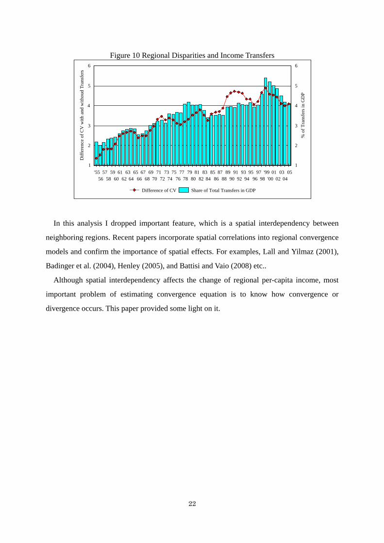
Figure 10 Regional Disparities and Income Transfers

In this analysis I dropped important feature, which is a spatial interdependency between

ne

capita income, most

im

'5556

5758

5960

6162

6364

6566

6768

6970

7172

7374

7576

7778

7980

8182

8384

8586

8788

8990

9192

9394

9596

9798

'99'00

0102

0304

051

2

3

4

5

6

Diff

eren

ce o

f CV

with

and

with

oud

Tran

sfer

s

1

2

3

4

5

6

% o

f Tra

nsfe

rs in

GD

P

Difference of CV Share of Total Transfers in GDP

ighboring regions. Recent papers incorporate spatial correlations into regional convergence

models and confirm the importance of spatial effects. For examples, Lall and Yilmaz (2001),

Badinger et al. (2004), Henley (2005), and Battisi and Vaio (2008) etc..

Although spatial interdependency affects the change of regional per-

portant problem of estimating convergence equation is to know how convergence or

divergence occurs. This paper provided some light on it.

22

References

Allington N.F.B. and McCombie J.S.L. (2007) Economic growth and beta-convergence in the east European transition economies, in Arestis eds. Economic Growth: New Direction in Theory and Policy, Edward Elgar, Massachusetts.

Armstrong H.W. (1995) Convergence among regions of the European Union, 1950-1990, Papers in Reg. Sci., 74, 143-152.

Badinger, H et al., (2003) Regional convergence in the European Union, 1985-1999: A Spatial Dynamic Panel Analysis,’ Regional Studies, 38, 3, 241-253, 2004(2003).

Barro R. and Sala-i-Martin X. (1996) Regional cohesion: Evidence and theories of regional growth and convergence, European Econ. Rev., 40, 1325-1352.

Barro R. and Sala-i-Martin X. (2004) Economic Growth, 2nd Edn. MIT Press, Cambridge, MA.

Battisiti M. and Di Vaio G. (2008) A spatially filtered mixture of convergenceβ − regression for EU regions, 1980-2002, Emp. Econ., 34, 105-121.

Carluer F. and Gaulier G. (2005) The impact of convergence in the industrial mix on regional comparative groth: Empirical evidence from the French case, Ann. Reg. Sci., 39, 85-105.

Crihfield J.B., J.F.Giertz, and S.Mehta (1995) Economic growth in the American States: the end of convergence? The Quart. Rev. of Econ. and Finance, 35, 551-577.

Chrihfield J. B. and Panggbean M.P.H. (1955) Growth and convergence in U.S. cities, J. Urban Econ., 38, 138-165.

Christopoulos, D.K. and Tsionas, E. (2004) Convergence and regional productivity differences: evidence from Greek prefectures, Ann. Reg. Sci., 38(3), 387-396.

Coulombe S. (2007) Globalization and Regional Disparity: A Canadian case study, Reg. Studies, 41, 1-17.

de la Fuente A. (2002) On the source of convergence: A close look at the Spanish regions, European Econ. Rev., 46, 569-599.

Desmet K. and Fafchamps M. (2006) Employment concentration across U.S. counties, Reg. Sci. Urban. Econ., 36, 482-509.

Dixon, R. and Thirlwall, A.P. (1975) A model of regional growth rate differences on Kaldorian lines, Oxford Econ. Papers, 27, 201-214.

Funke M. and Strulik H. (1999) Regional growth in West Germany: convergence or divergence? Econo. Modelling, 16, 489-502.

Hammond G.W. (2006) A time series analysis of U.S. metropolitan and non-metropolitan income divergence, Ann. Reg. Sci., 40, 8-94.

Helliwell, J. F., ‘Convergence and Migration among Provinces,’ Canadian Journal of Economics, 29, S324-S330, 1996.

Henley A. (2005) On regional growth convergence in Great Britain, Reg. Studies, 39, 1245-1260.

Kosfeld R. et al. (2006) Regional productivity and income convergence in the United

23

24

Germany, 1992-2000,’ Reg. Studies, 40, 755-767. Lall S.V. and Yilmaz S. (2001) Regional economic convergence: Do policy instruments make

a difference? Ann. Reg. Sci., 35, 153-166. Miller J.R. and Genc I. (2005) Alternative regional specification and convergence of U.S.

regional growth rates, Ann. Reg. Sci., 39, 241-253. Nijkamp P. and Poot J. (1998) Spatial perspectives on new theories of economic growth, Ann.

Reg. Sci., 32, 7-37. Terrasi M. (1999) Convergence and divergence across Italian regions, Ann. Reg. Sci., 33,

491-510. Wang Z. and Z. Ge (2004) Convergence and transition auspice of Chinese regional growth,

Ann. Reg. Sci., 38, 727-739. Webber D.J. and White P. (2003) Regional Factor price convergence across four major

European countries, Reg. Studies, 37, 773-782.