Heuristic procedures for solving the General Assembly Line Balancing Problem with Setups (GALBPS) Luigi Martino and Rafael Pastor EOLI: Enginyeria d’Organització i Logística Industrial IOC-DT-P-2007-15 Desembre 2007

1

Heuristic procedures for solving the General Assembly Line Balancing Problem with Setups (GALBPS)ϒ

Luigi Martino and Rafael Pastor*

IOC Research Institute Technical University of Catalonia

Av. Diagonal 647, 11th floor, 08028, Barcelona, Spain luigi.martino@gmx.de / rafael.pastor@upc.edu

Abstract: The General Assembly Line Balancing Problem with Setups (GALBPS) was recently defined in the literature. It adds sequence-dependent setup time considerations to the classical Simple Assembly Line Balancing Problem (SALBP) as follows: whenever a task is assigned next to another at the same workstation, a setup time must be added to compute the global workstation time, thereby providing the task sequence inside each workstation. This paper proposes over 50 priority-rule-based heuristic procedures to solve GALBPS, many of which are an improvement upon heuristic procedures published to date.

Keywords: assembly line balancing, sequence-dependent setup times

1. Introduction Assembly lines are components of many production systems, such as those used in the automotive and household appliance industries. The problem of designing and balancing assembly lines is very difficult to solve due to its combinatorial nature—it is NP-hard (see, e.g., Wee and Magazine, 1982)—and to the numerous tasks and constraints characteristic of real-life situations. The classic Assembly Line Balancing Problem (ALBP) basically consists of assigning a set of tasks (each characterized by its processing time) to an ordered sequence of workstations, such that the precedence constraints between tasks are maintained and a given efficiency measure is optimized. The problem of designing and balancing assembly lines has been examined extensively in the literature. A number of overviews have been published, including Baybars (1986), Ghosh and Gagnon (1989), Erel and Sarin (1998), Scholl (1999), Rekiek et al. (2002), Becker and Scholl (2006), Scholl and Becker (2006) and Boysen et al. (2007). However, most of these papers focus on the simple ALBP (SALBP). This problem has been approached using heuristic procedures (e.g., Talbot et al. (1986), and Ponnambalam et al. (1999)) as well exact procedures (e.g., Talbot and Patterson (1984), Kao and Queyranne (1982), and Scholl and Klein (1997)). Myriad complex cases have been examined, including problems that consider lines with parallel workstations or parallel tasks; mixed or multi-models; multiple products; U-shaped, two-sided, buffered or parallel lines; incompatibility between tasks; stochastic processing times; and equipment selection (e.g., Park et al. (1997), Miltenburg (2001), Pastor et al. (2002), Ağpak and Gökçen (2005), Amen (2006), Corominas et al. (2006), Gamberini et al. (2006), Gökçen et al. (2006) or Capacho and Pastor (2007)). Consequently, generalized problems have garnered much interest. ϒ This work was developed under research project DELIMER (DPI2004-03472), which is supported by the Spanish National Science and Technology Commission (CICYT) and co-financed by FEDER. * Corresponding author: Rafael Pastor, IOC Research Institute, Av. Diagonal, 647 (edif. ETSEIB), p. 11, 08028 Barcelona, Spain; Tel. + 34 93 401 17 01; fax + 34 93 401 66 05; e-mail: rafael.pastor@upc.edu.

2

Articles on assembly line balancing typically focus on the problem in a pure sense—as if, once the tasks were assigned to the workstations, there was nothing left to do. However, in some real production lines, the sequence in which tasks are executed inside the workstation is very important, since there are sequence-dependent setup times between tasks. Andrés et al. (2008) introduced, modelled and solved the General Assembly Line Balancing Problem with Setups (GALBPS). GALBPS not only requires that the assembly line has to be balanced, but also that the sequence of tasks assigned to every workstation must be defined (due to the existence of sequence-dependent setup times). Therefore, both the inter-station balancing and intra-station task sequencing must be solved simultaneously. This reflects a more realistic scenario for many assembly lines, especially those from the electronics industry or similar sectors featuring low cycle times. Andrés et al. (2008) employed a binary programming model which only provides optimal solutions for very small instances. The authors described eight different heuristic rules which were designed based on task-oriented and workstation-oriented strategies with different criteria for task-selection ordering. Finally, they presented a GRASP algorithm, and then evaluated it against the heuristic rules through an experimental study. In this paper, we propose over 50 heuristic procedures, based on priority rules, for solving GALBPS. Many of these procedures improve upon those published to date. The remainder of the paper is organized as described below. GALBPS is outlined in Section 2, and the heuristic procedures designed to solve it are explained in Section 3. These heuristic procedures were tested and evaluated through a computational experiment, the main results of which are presented in Section 4. Since there is no standard benchmark for this novel problem, the experimental study was carried out with a set of self-made instances generated from the well-known set of instances available on Scholl’s & Klein's homepage for assembly line balancing research (www.assembly-line-balancing.de). Finally, conclusions on this work and ideas for further research are presented in Section 5. 2. The General Assembly Line Balancing Problem with Setups GALBPS adds sequence-dependent setup time considerations to the classical Simple Assembly Line Balancing Problem (SALBP) as follows: whenever a task j is assigned next to another task i at the same workstation, a setup time ,i jτ must be added to compute the global workstation time, thereby providing the task sequence inside each workstation. Furthermore, if a task p is the last one assigned to the workstation in which task i was the first task assigned, then a setup time ,p iτ must also be considered. This is because the tasks are repeated cyclically; the last task in one cycle of the workstation is performed just before the first task in the next cycle. As an example, we can take a case in which there are three tasks (A, B and C) assigned to a workstation and having processing times ( it ) of 10At = , 12Bt = and 9Ct = , respectively. Moreover, we consider that are no precedence constraints between the

3

tasks, and that the setup times ( ),i jτ are the following: , 3A Bτ = , , 4A Cτ = , , 2B Aτ = ,

, 1B Cτ = , , 3C Aτ = and , 4C Bτ = . Table 1 shows two possible sequences for the three tasks, with the times to be considered as well as the global workstation time (which equals the sum of all processing times and setup times). As observed, the two solutions differ by three units of time.

Sequence Times to be considered Global workstation time A-B-C 10+3+12+1+9+3 38 B-A-C 12+2+10+4+9+4 41

Table 1. Two possible sequences for the tasks A, B and C In most industrial assembly lines these setup times exist but are usually not considered because they are very short compared to processing times. In certain cases, the setup times do not depend on the sequence of tasks, and are added to the processing times of the tasks. In other cases, the task sequence for every workstation is defined only after the tasks have been assigned and the line has subsequently been balanced; the problem is therefore solved in two separate stages. However, a better strategy to solve GALBPS is to simultaneously solve the line-balancing and the task-sequencing problems. Andrés et al. (2008) provided different real examples of GALBPS, including that of workers using different tools for different tasks and that of robotic lines. What is important in this situation is to define the best work sequence for the worker in order to minimize the global workstation time, including setup times. Robotic lines are another real case: often, the robot must remove one tool, select the corresponding new tool from a set and then make adjustments before starting the next assigned task. As mentioned in Graves and Lamar (1983), tool changes are especially important in robotic assembly because they may involve times that are comparable in magnitude to operation times. Another practical case is that in which components are located in separate containers: the time required to get to one container depends on the last component that was assembled for the product, meaning that the work sequence inside the workstation is significant. An overview of the relevant literature reveals a shortage of publications on this topic. On the one hand, we have focused on literature about scheduling research involving setup considerations (Allahverdi et al., 1999, 2006), but we were unable to find any references to evaluation of the work sequence inside the assembly line. On the other hand, we referred to the surveys on problems and methods in assembly line balancing (Baybars [1986]; Ghosh and Gagnon [1989]; Erel and Sarin [1998]; Scholl [1999]; Rekiek et al. [2002]; Becker and Scholl [2006]; and Scholl and Becker [2006]). In these, setup times are only included when mixed-model and multi-model lines are considered. However, in both cases the sequence refers to the products or models to be assembled on the line, not to the work sequence of tasks inside the workstations. In Merengo et al. (1999) both the line balancing problem and the sequencing problem are tackled separately for mixed-model assembly lines, whereas in Sawik (2002) both problems are handled simultaneously for the specific case of printed circuit board production lines.

4

One survey which does include the sequence-dependent task time increments is Boysen et al. (2007), p. 679, in which it is stated that “If two tasks are executed at a station one directly after the other, additional time might be required for setup operations or tool changes (Wilhelm, 1999) and repositioning of workpieces (Arcus, 1966; Bautista and Pereira, 2002)”. In Wilhelm (1999) the assembly system design problem with tool changes (ASDPTCs) is presented, and then solved by a column-generation approach. The objective is to minimize the cost of assigning machines, tooling and tasks (including loading and unloading tasks as well as tool changes) to workstations. In contrast to other methods, this column-generation approach calculates the optimal assembly sequence at each workstation, including tool-change time and cost. In Arcus (1966) the assembly line problem is first analyzed in its simple form, and then in its complex form, which includes consideration of additional times that depend on the sequence of tasks: obtaining tools, or changing the position of a worker or of a unit. In Bautista and Pereira (2002) a real problem from a bicycle assembly line is solved using an ant algorithm metaheuristic. This case includes division of tasks between right and left sides, depending on which side of the chassis the task must be performed. As the chassis is moved along the line by a platform, turning the bicycle involves a setup time between tasks from different sides of the platform. In Boysen et al. (2007), p. 679, it is also stated that “Indirect sequence-dependent time increments occur if the status achieved by completing particular tasks has an effect on the processing time of other tasks which are executed later in the same or another station (Scholl et al., 2006)”. This problem is handled in Scholl et al. (2006), in which the sequence-dependent assembly line balancing problem (SDALBP) is defined, and in Capacho and Pastor (2007), in which the Alternative Subgraphs Assembly Line Balancing Problem (ASALBP) is introduced. However, the aforementioned problem is not the same as the problem at hand: in GALBPS a setup time ,i jτ must be considered whenever a task j is assigned next to another i at the same workstation. As explained above, in Andrés et al. (2008) GALBPS is modelled through a binary programming model, eight different heuristic rules are designed, and finally, a GRASP algorithm is presented and evaluated. Finally, Agnetis and Arbib (1997) face a related problem, whereby the task precedence network is ‘comb’ shaped. This means that the operations leading to the different parts of the final product are first performed separately, and then subsequently assembled in a later stage. The problem consists of assigning operations to machines, and then sequencing them in every workstation to maximize defined performance indicators. Having the special ‘comb’ precedence network greatly reduces the combinatorial nature of the problem, enabling it to be solved in polynomial time. For a cyclic case in which the tasks p and i are the last and first assigned to a given workstation, respectively, then a setup time ,p iτ must be also considered. However, the majority of works cited above do not apply it. Moreover, only Andrés et al. (2008) describe rapid and facile solution procedures that can be applied by any practitioner. As in the classification of Baybars (1986), when the objective is to minimize the number of workstations for a given upper bound on the cycle time, the problem is referred to as GALBPS-1; when the objective is to minimize the cycle time given a

5

number of workstations, the problem is called GALBPS-2. Herein are presented improved heuristic procedures based on priority rules to solve GALBPS-1. 3. The heuristic procedures SALBP is known to be NP-hard; since SALBP is only one special case of GALBPS in which setup times do not exist, then GALBPS is also NP-hard. Hence, the use of heuristic methods to obtain good results at the computational speed required of real industrial environments is fully justified. In ALBP, most heuristic algorithms are based on generating feasible solutions by successively assigning tasks, or subsets of tasks, to workstations. Therefore, these algorithms consider partial solutions containing a number of assigned tasks and (partial) workstation loads, whereas the remaining tasks and workstation idle times constitute a residual problem (Scholl and Becker, 2006). The aim is to assign tasks to workstations and sequence them such that no precedence relationships are violated, and the value global time (including setup times) is less than the cycle time. Almost every solution procedure is based on one of the two following construction schemes, which define the main way of assigning tasks to workstations: Workstation-oriented assignment: In any step of the procedure a single available task is selected and then assigned to workstation k which is being completed, such that a complete load of assignable tasks is built for k before the next workstation 1k + is considered. Task-oriented assignment: In any step of the procedure a single available task is selected and then assigned to a workstation to which it can be assigned. This Section is organized as follows: the terminology used is presented (Subsection 3.1); the workstation-oriented procedure and designed simple heuristic rules are described (Subsection 3.2); use of the task-oriented procedure and designed simple heuristic rules for said procedure are explained (Subsection 3.3); and finally, new, more elaborate workstation-oriented procedures are introduced (Subsection 3.4). 3.1. Terminology The principal data and parameters used are described below: ,i j index for the tasks

k index for the workstations N number of tasks ( )1,...,i N= TC upper bound on the cycle time

iS set of successor tasks, at any step, of the task i

iP set of preceding tasks, at any step, of the task i

iNS number of successor tasks, at any step, of the task i ( )i iNS S=

iNIS number of immediate successors of task i

it processing time of task i

6

,i jτ setup time when task j is performed directly after task i inside the same workstation, assuming that , 0i iτ =

,last iτ setup time between the last task assigned to the workstation which is being completed and the task i

,i firstτ setup time between the task i and first task assigned to the workstation which is being completed

iτ average setup time of the task i (between i and either its successor or preceding tasks, at any step)

,i iE L earliest and latest workstation, respectively, to which task i can be assigned to; before assigning a task, the total time of the preceding tasks must be assigned and, likewise, after assigning a task, the total time of its successors must be assigned. The range of workstations [ ],i iE L to which task i can be assigned

(see, e.g., Scholl, 1999) is thereby obtained. The range [ ],i iE L is more restricted in this work, due to it is considered the minimum number of setup times between the task i and either its successor or preceding tasks.

3.2. Workstation-oriented procedure (WH ) The workstation-oriented procedure (WH ) is an iterative procedure which, at each iteration and according to a priority rule, assigns one of a group of candidate tasks to the workstation k which is being completed. A task i is considered a candidate once its preceding tasks have been assigned and it fits in the workstation k . If there are no candidate tasks available, but there are still tasks left to assign, then k is closed, and workstation 1k + is opened. The procedure ends once all of the tasks have been assigned. A vital element in the definition of the WH procedure is the definition of the priority rule, which orders the candidate tasks at the time of choosing the next task to be assigned. Table 2 lists the 38 priority rules used in the WH procedure (denoted R01 to R38). In all cases, the task *x is assigned with * max ix i

v v= . The priority rules R01 to

R15, which do not take into account setup times between tasks, have been reported in the literature for the SALBP: R01 (Moodie and Young, 1965); R02, R05, and R08 to R13 (Talbot and Patterson, 1984); R03 (Tonge, 1961); R04 (Helgeson and Birnie, 1961); R06 and R07 (Arcus, 1963); R14 (Bhattacharjee and Sahu, 1988); and R15 (e.g. Boctor, 1995). Rules R16 to R19 are described for GALBPS in Andrés et al. (2008). Rules R20 to R38 are new rules developed in this work. Priority rules R01 to R15, which do not take into account setup times between tasks, were nevertheless used to determine the influence of setup times at the time of selecting tasks. The new rules (R20 to R38) are based on taking into account the elements of the priority rules for SALBP described in the literature (i.e. it , i , iNS , iNIS ,

i

jj S

t∈∑ , iE and

iL ), as well as the setup times between tasks ( ,last iτ , ,i firstτ and iτ ). For example, according to R28, the highest priority task is the one having the greatest ratio of processing time to the setup time between itself and the last task assigned to the workstation which is being completed.

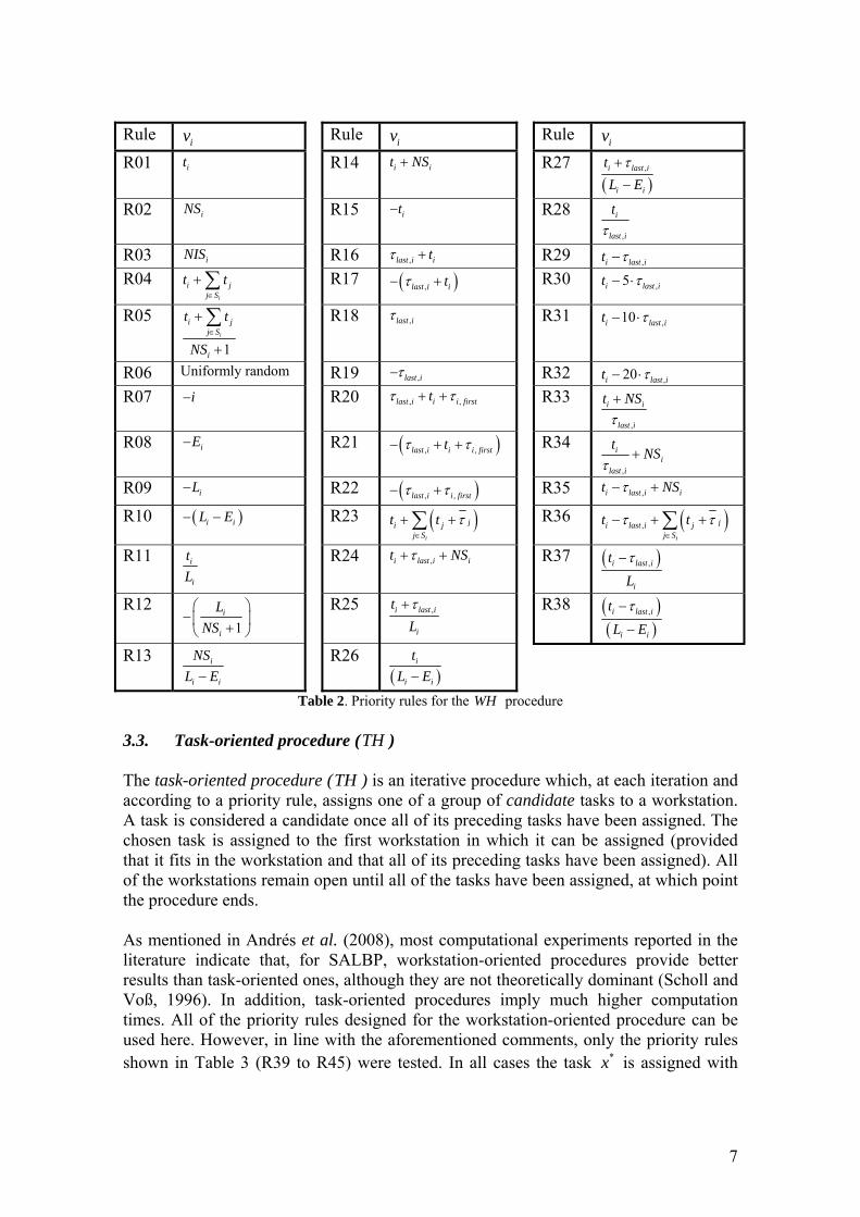
7

Rule iv Rule iv Rule iv R01 it R14 i it NS+ R27

( ),i last i

i i

tL Eτ+−

R02 iNS R15 it− R28 ,

i

last i

tτ

R03 iNIS R16 ,last i itτ + R29 ,i last it τ− R04

i

i jj S

t t∈

+ ∑ R17 ( ),last i itτ− + R30 ,5i last it τ− ⋅

R05

1i

i jj S

i

t t

NS∈

+

+

∑

R18 ,last iτ R31 ,10i last it τ− ⋅

R06 Uniformly random R19 ,last iτ− R32 ,20i last it τ− ⋅ R07 i− R20 , ,last i i i firsttτ τ+ + R33

,

i i

last i

t NSτ+

R08 iE− R21 ( ), ,last i i i firsttτ τ− + + R34 ,

ii

last i

tNS

τ+

R09 iL− R22 ( ), ,last i i firstτ τ− + R35 ,i last i it NSτ− +

R10 ( )i iL E− − R23 ( )i

ji jj S

t t τ∈

+ +∑ R36 ( ),i

ji last i jj S

t tτ τ∈

− + +∑

R11 i

i

tL

R24 ,i last i it NSτ+ + R37 ( ),i last i

i

tLτ−

R12 1

i

i

LNS

⎛ ⎞−⎜ ⎟+⎝ ⎠

R25 ,i last i

i

tLτ+ R38 ( )

( ),i last i

i i

tL Eτ−

−

R13 i

i i

NSL E−

R26 ( )

i

i i

tL E−

Table 2. Priority rules for the WH procedure 3.3. Task-oriented procedure (TH ) The task-oriented procedure (TH ) is an iterative procedure which, at each iteration and according to a priority rule, assigns one of a group of candidate tasks to a workstation. A task is considered a candidate once all of its preceding tasks have been assigned. The chosen task is assigned to the first workstation in which it can be assigned (provided that it fits in the workstation and that all of its preceding tasks have been assigned). All of the workstations remain open until all of the tasks have been assigned, at which point the procedure ends. As mentioned in Andrés et al. (2008), most computational experiments reported in the literature indicate that, for SALBP, workstation-oriented procedures provide better results than task-oriented ones, although they are not theoretically dominant (Scholl and Voß, 1996). In addition, task-oriented procedures imply much higher computation times. All of the priority rules designed for the workstation-oriented procedure can be used here. However, in line with the aforementioned comments, only the priority rules shown in Table 3 (R39 to R45) were tested. In all cases the task *x is assigned with

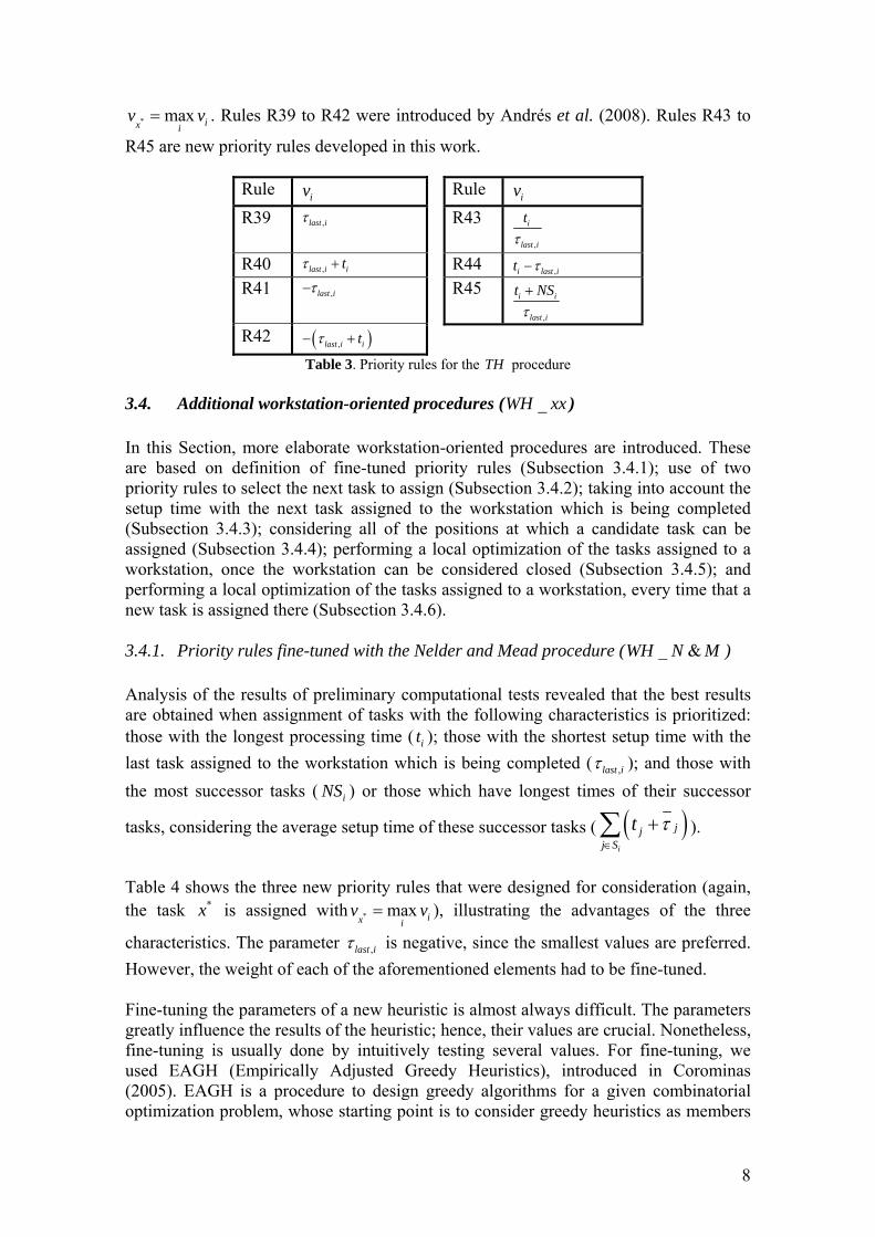
8

* max ix iv v= . Rules R39 to R42 were introduced by Andrés et al. (2008). Rules R43 to

R45 are new priority rules developed in this work.

Rule iv Rule iv R39 ,last iτ R43

,

i

last i

tτ

R40 ,last i itτ + R44 ,i last it τ− R41 ,last iτ− R45

,

i i

last i

t NSτ+

R42 ( ),last i itτ− + Table 3. Priority rules for the TH procedure

3.4. Additional workstation-oriented procedures ( _WH xx ) In this Section, more elaborate workstation-oriented procedures are introduced. These are based on definition of fine-tuned priority rules (Subsection 3.4.1); use of two priority rules to select the next task to assign (Subsection 3.4.2); taking into account the setup time with the next task assigned to the workstation which is being completed (Subsection 3.4.3); considering all of the positions at which a candidate task can be assigned (Subsection 3.4.4); performing a local optimization of the tasks assigned to a workstation, once the workstation can be considered closed (Subsection 3.4.5); and performing a local optimization of the tasks assigned to a workstation, every time that a new task is assigned there (Subsection 3.4.6). 3.4.1. Priority rules fine-tuned with the Nelder and Mead procedure ( _ &WH N M ) Analysis of the results of preliminary computational tests revealed that the best results are obtained when assignment of tasks with the following characteristics is prioritized: those with the longest processing time ( it ); those with the shortest setup time with the last task assigned to the workstation which is being completed ( ,last iτ ); and those with the most successor tasks ( iNS ) or those which have longest times of their successor

tasks, considering the average setup time of these successor tasks ( ( )i

jjj S

t τ∈

+∑ ).

Table 4 shows the three new priority rules that were designed for consideration (again, the task *x is assigned with * max ix i

v v= ), illustrating the advantages of the three

characteristics. The parameter ,last iτ is negative, since the smallest values are preferred. However, the weight of each of the aforementioned elements had to be fine-tuned. Fine-tuning the parameters of a new heuristic is almost always difficult. The parameters greatly influence the results of the heuristic; hence, their values are crucial. Nonetheless, fine-tuning is usually done by intuitively testing several values. For fine-tuning, we used EAGH (Empirically Adjusted Greedy Heuristics), introduced in Corominas (2005). EAGH is a procedure to design greedy algorithms for a given combinatorial optimization problem, whose starting point is to consider greedy heuristics as members

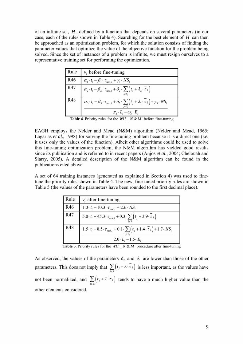
9

of an infinite set, H , defined by a function that depends on several parameters (in our case, each of the rules shown in Table 4). Searching for the best element of H can then be approached as an optimization problem, for which the solution consists of finding the parameter values that optimize the value of the objective function for the problem being solved. Since the set of instances of a problem is infinite, we must resign ourselves to a representative training set for performing the optimization.

Rule iv before fine-tuning R46 1 1 , 1i last i it NSα β τ γ⋅ − ⋅ + ⋅ R47 ( )2 2 , 2 2

i

ji last i jj S

t tα β τ δ λ τ∈

⋅ − ⋅ + ⋅ + ⋅∑

R48 ( )3 3 , 3 3 3

3 3

i

ji last i j ij S

i i

t t NS

L E

α β τ δ λ τ γ

π ω∈

⋅ − ⋅ + ⋅ + ⋅ + ⋅

⋅ − ⋅

∑

Table 4. Priority rules for the _ &WH N M before fine-tuning EAGH employs the Nelder and Mead (N&M) algorithm (Nelder and Mead, 1965; Lagarias et al., 1998) for solving the fine-tuning problem because it is a direct one (i.e. it uses only the values of the function). Albeit other algorithms could be used to solve this fine-tuning optimization problem, the N&M algorithm has yielded good results since its publication and is referred to in recent papers (Anjos et al., 2004; Chelouah and Siarry, 2005). A detailed description of the N&M algorithm can be found in the publications cited above. A set of 64 training instances (generated as explained in Section 4) was used to fine-tune the priority rules shown in Table 4. The new, fine-tuned priority rules are shown in Table 5 (the values of the parameters have been rounded to the first decimal place).

Rule iv after fine-tuning R46 ,1.0 10.3 2.6i last i it NSτ⋅ − ⋅ + ⋅ R47 ( ),5.0 45.3 0.3 3.9

i

ji last i jj S

t tτ τ∈

⋅ − ⋅ + ⋅ + ⋅∑

R48 ( ),1.5 8.5 0.1 1.4 1.7

2.0 1.5i

ji last i j ij S

i i

t t NS

L E

τ τ∈

⋅ − ⋅ + ⋅ + ⋅ + ⋅

⋅ − ⋅

∑

Table 5. Priority rules for the _ &WH N M procedure after fine-tuning As observed, the values of the parameters 2δ and 3δ are lower than those of the other

parameters. This does not imply that ( )i

jjj S

t λ τ∈

+ ⋅∑ is less important, as the values have

not been normalized, and ( )i

jjj S

t λ τ∈

+ ⋅∑ tends to have a much higher value than the

other elements considered.

10

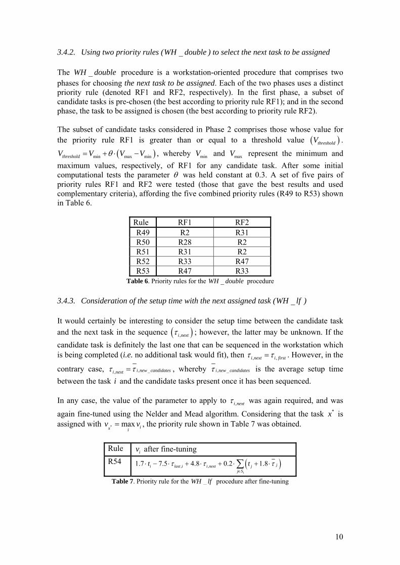
3.4.2. Using two priority rules ( _WH double ) to select the next task to be assigned The _WH double procedure is a workstation-oriented procedure that comprises two phases for choosing the next task to be assigned. Each of the two phases uses a distinct priority rule (denoted RF1 and RF2, respectively). In the first phase, a subset of candidate tasks is pre-chosen (the best according to priority rule RF1); and in the second phase, the task to be assigned is chosen (the best according to priority rule RF2). The subset of candidate tasks considered in Phase 2 comprises those whose value for the priority rule RF1 is greater than or equal to a threshold value ( )thresholdV .

( )min max minthresholdV V V Vθ= + ⋅ − , whereby minV and maxV represent the minimum and maximum values, respectively, of RF1 for any candidate task. After some initial computational tests the parameter θ was held constant at 0.3. A set of five pairs of priority rules RF1 and RF2 were tested (those that gave the best results and used complementary criteria), affording the five combined priority rules (R49 to R53) shown in Table 6.

Rule RF1 RF2 R49 R2 R31 R50 R28 R2 R51 R31 R2 R52 R33 R47 R53 R47 R33

Table 6. Priority rules for the _WH double procedure 3.4.3. Consideration of the setup time with the next assigned task ( _WH lf ) It would certainly be interesting to consider the setup time between the candidate task and the next task in the sequence ( ),i nextτ ; however, the latter may be unknown. If the candidate task is definitely the last one that can be sequenced in the workstation which is being completed (i.e. no additional task would fit), then , ,i next i firstτ τ= . However, in the

contrary case, , _, i new candidatesi nextτ τ= , whereby , _i new candidatesτ is the average setup time between the task i and the candidate tasks present once it has been sequenced. In any case, the value of the parameter to apply to ,i nextτ was again required, and was

again fine-tuned using the Nelder and Mead algorithm. Considering that the task *x is assigned with * max ix i

v v= , the priority rule shown in Table 7 was obtained.

Rule iv after fine-tuning R54 ( ), ,1.7 7.5 4.8 0.2 1.8

i

ji last i i next jj S

t tτ τ τ∈

⋅ − ⋅ + ⋅ + ⋅ + ⋅∑

Table 7. Priority rule for the _WH lf procedure after fine-tuning

11

R54 was designed considering R47, which provided the best results among the three priority rules fine-tuned with the Nelder and Mead algorithm (as explained in Section 4). 3.4.4. The position at which a candidate task can be assigned to ( _WH pos ) In the WH procedure, a task i is always assigned after the last task assigned to the workstation k which is being completed. Completion of said condition yields a set of candidate tasks and enables calculation of the priority rule associated with each of them. In the _WH pos procedure, a task i can also be assigned to intermediate positions in the partial task sequence that have already been assigned to the workstation k . Obviously, in this case precedence among tasks must be respected, and, considering the setup times for assigning a task i to position s of the sequence, the task i must fit in the workstation k . A task i can thereby have different values for the priority rule (as long as the rule accounts for setup times): one value for each possible position s of the sequence in which i can be assigned. The greatest value of the priority rule is assigned to the task i for all possible positions s at which i can be assigned. In the event of a tie, the position s which corresponds to the lowest value of the sum of the setup time with the previous task in the sequence, the processing time, and the setup time with the following task in the sequence is assigned. As may be deduced, the number of candidate tasks can—and does—increase: once a non-candidate task is sequenced after the last assigned task, it can become a candidate when it is assigned to an intermediate position of the partial sequence of already assigned tasks. A set of six priority rules (R01, R02, R28, R29, R33 and R47) which gave good results and used complementary criteria were tested with the _WH pos procedure. 3.4.5. Local optimization of the tasks assigned to a workstation ( _WH swap ) The _WH swap procedure consists of performing local optimization of the sequence of tasks assigned to the workstation k which has just closed because no additional tasks can fit, before opening a new workstation 1k + . As a result of said optimization, the tasks assigned to the workstation k can be tracked (i.e. candidate tasks reappear). The procedure used for local optimization consists of iteratively calculating all of the neighbouring sequences of a given sequence ( )currentSeq and then substituting currentSeq

with the best neighbouring sequence ( )_best neicurrentSeq . The local optimization continues as

long as _best neicurrentSeq is better than currentSeq , and stops once _best nei

currentSeq is not better than

currentSeq . For a given sequence currentSeq , only feasible neighbouring sequences are considered. A sequence 1Seq is considered to be better than another sequence 2Seq , if it has a shorter total required time (the sum of processing and setup times) than 2Seq . The neighbouring sequences of currentSeq are generated by swapping the tasks assigned to every pair of its consecutive positions in the workstation k .

12

_WH swap was tested with the same priority rules used to test _WH pos : R01, R02,

R28, R29, R33 and R47. 3.4.6. Local optimization of the tasks assigned to a workstation after each assignment ( _WH opt ) The _WH opt procedure consists of performing a local optimization of the sequence of tasks assigned to a workstation every time that a new task is assigned there—in other words, unlike the case of _WH swap , local optimization is performed without having to wait for the workstation to close. _WH opt differs from _WH swap in that the neighbouring sequences of currentSeq are generated by inserting every task assigned to the workstation k at each possible position of the sequence. In the _WH opt procedure, in order to increase the number of candidate tasks, a task i is initially assigned after the last task assigned to the workstation k , and then the local optimization described in the previous paragraph is immediately performed. This differs from the procedure WH (whereby the task i is assigned after the last task assigned to the workstation k which is being completed), and from the procedure _WH pos (in which the task i is assigned to the intermediate positions of the partial sequence of tasks already assigned to the workstation k ). Here, only feasible sequences are considered. The number of candidate tasks can and does increase: a non-candidate task, having not been sequenced in any position of the partial sequence of already assigned tasks, can become a candidate upon execution of the local optimization.

_WH opt was tested with the same priority rules used to test _WH pos and _WH swap : R01, R02, R28, R29, R33 and R47.

4. Computational experiment The heuristic procedures proposed in Section 3 were tested with a set of self-made instances. The results demonstrate that some of the new heuristic procedures based on priority rules improve upon those described to date, including the metaheuristic GRASP proposed by Andrés et al. (2008). This Section is broken down as follows: the method used to generate the set of benchmark instances is detailed (Subsection 4.1); a lower bound on GALBPS and a GRASP metaheuristic both defined by Andrés et al. (2008) are briefly introduced (Subsection 4.2 and 4.3); and lastly, commentary on the results of the computational experiment is provided (Subsection 4.4). 4.1. Generation of benchmark instances Since GALBPS is a novel problem, there is no set of benchmark instances with setup times available for testing. Therefore a set of self-made instances was generated from a well-known set of problems obtained from Scholl's and Klein's assembly line balancing

13

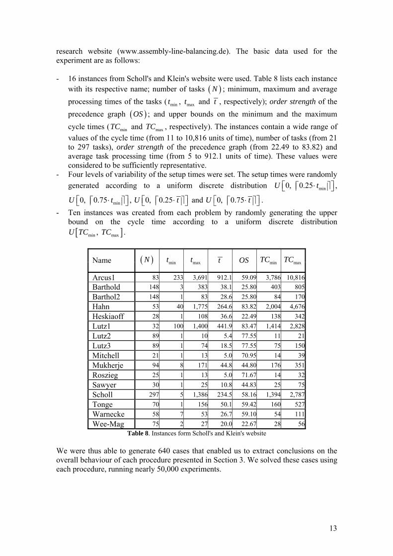
research website (www.assembly-line-balancing.de). The basic data used for the experiment are as follows: - 16 instances from Scholl's and Klein's website were used. Table 8 lists each instance

with its respective name; number of tasks ( )N ; minimum, maximum and average processing times of the tasks ( mint , maxt and t , respectively); order strength of the precedence graph ( )OS ; and upper bounds on the minimum and the maximum cycle times ( minTC and maxTC , respectively). The instances contain a wide range of values of the cycle time (from 11 to 10,816 units of time), number of tasks (from 21 to 297 tasks), order strength of the precedence graph (from 22.49 to 83.82) and average task processing time (from 5 to 912.1 units of time). These values were considered to be sufficiently representative.

- Four levels of variability of the setup times were set. The setup times were randomly generated according to a uniform discrete distribution min0, 0.25U t⎡ ⋅ ⎤⎡ ⎤⎢ ⎥⎣ ⎦ ,

min0, 0.75U t⎡ ⋅ ⎤⎡ ⎤⎢ ⎥⎣ ⎦ , 0, 0.25U t⎡ ⋅ ⎤⎡ ⎤⎢ ⎥⎣ ⎦ and 0, 0.75U t⎡ ⋅ ⎤⎡ ⎤⎢ ⎥⎣ ⎦ . - Ten instances was created from each problem by randomly generating the upper

bound on the cycle time according to a uniform discrete distribution [ ]min max, U TC TC .

Name ( )N mint maxt t OS minTC maxTC

Arcus1 83 233 3,691 912.1 59.09 3,786 10,816Barthold 148 3 383 38.1 25.80 403 805Barthol2 148 1 83 28.6 25.80 84 170Hahn 53 40 1,775 264.6 83.82 2,004 4,676Heskiaoff 28 1 108 36.6 22.49 138 342Lutz1 32 100 1,400 441.9 83.47 1,414 2,828Lutz2 89 1 10 5.4 77.55 11 21Lutz3 89 1 74 18.5 77.55 75 150Mitchell 21 1 13 5.0 70.95 14 39Mukherje 94 8 171 44.8 44.80 176 351Roszieg 25 1 13 5.0 71.67 14 32Sawyer 30 1 25 10.8 44.83 25 75Scholl 297 5 1,386 234.5 58.16 1,394 2,787Tonge 70 1 156 50.1 59.42 160 527Warnecke 58 7 53 26.7 59.10 54 111Wee-Mag 75 2 27 20.0 22.67 28 56

Table 8. Instances form Scholl's and Klein's website We were thus able to generate 640 cases that enabled us to extract conclusions on the overall behaviour of each procedure presented in Section 3. We solved these cases using each procedure, running nearly 50,000 experiments.

14

4.2. A lower bound on GALBPS A lower bound on GALBPS, GALBPSLB , was used to evaluate the efficiency of the proposed heuristic procedures. The lower bound used was that proposed by Andrés et al. (2008), 1GALBPSLB , which is an adaptation of the most common lower bound on SALBP. Further details on 1GALBPSLB can be found in Andrés et al. (2008). 4.3. GRASP metaheuristic for GALBPS (from Andrés et al., 2008) The GRASP (Greedy Randomized Adaptative Search Procedure) metaheuristic, first described by Feo and Resende (1995) and used in Andrés et al. (2008), is one of the most efficient heuristic procedures for solving GALBPS published to date. It involves two steps: constructing a solution and improving it. The two steps are repeated a prescribed number of times, _NS GRASP . We programmed GRASP to compare its efficiency to that of our new heuristic procedures. The GRASP metaheuristic of Andrés et al. (2008) is summarised below (for a more detailed explanation, see Andrés et al., 2008). In the first phase, in which an initial solution is constructed, two greedy procedures were used: the procedure used in Andrés et al. (2008), which corresponds to the WH procedure with the priority rule R16; and the WH procedure with the priority rule R47, which, as it can be seen in Subsection 4.4, is one of the procedures which yields the best results. The second phase, in which the solution is improved, comprised a local optimization procedure similar to that described for the _WH swap procedure: all of the neighbouring solutions of a given solution ( )currentSol are iteratively generated, and then

currentSol is substituted with the best neighbouring solution ( )_best neicurrentSol , as long as the

latter is better than the former. The process stops once _best neicurrentSol is no better than

currentSol . The neighbouring solutions of currentSol are generated by swapping the tasks assigned to each pair of consecutive positions of the complete sequence of tasks with which it can be described. It should be noted that in this case, as opposed to that of

_WH swap , the tasks assigned to different workstations can be also interchanged.

_NS GRASP (the number of times that the two steps are repeated) is equal to 5, which provides a computational time comparable to that of computationally-intensive heuristic procedures (TH procedures). 4.4. Results of the computational experiment We evaluated the performance of the heuristic procedures in order to identify the best one. The solutions obtained by using each heuristic procedure for each instance were compared. The results are shown in Table 9, in which the following notation is used: TofP , type of procedure; Rule , priority rule used; ∆ , average relative deviation from the value of the best solution BS (for each instance, BS is the value of the best of all solutions found by the heuristic procedures, and ∆ is computed, for each heuristic

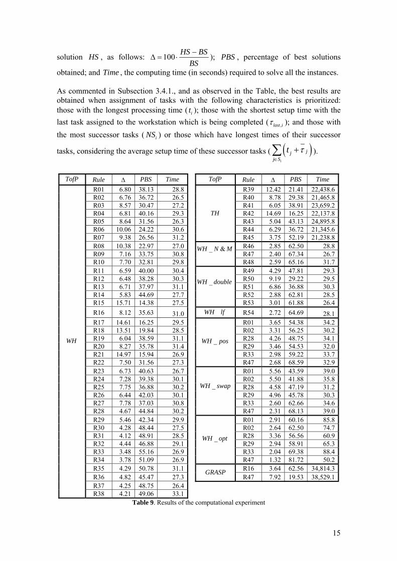
15

solution HS , as follows: 100 HS BSBS−

∆ = ⋅ ); PBS , percentage of best solutions

obtained; and Time , the computing time (in seconds) required to solve all the instances. As commented in Subsection 3.4.1., and as observed in the Table, the best results are obtained when assignment of tasks with the following characteristics is prioritized: those with the longest processing time ( it ); those with the shortest setup time with the last task assigned to the workstation which is being completed ( ,last iτ ); and those with the most successor tasks ( iNS ) or those which have longest times of their successor

tasks, considering the average setup time of these successor tasks ( ( )i

jjj S

t τ∈

+∑ ).

TofP Rule ∆ PBS Time TofP Rule ∆ PBS Time

R01 6.80 38.13 28.8 R39 12.42 21.41 22,438.6R02 6.76 36.72 26.5 R40 8.78 29.38 21,465.8R03 8.57 30.47 27.2 R41 6.05 38.91 23,659.2R04 6.81 40.16 29.3 R42 14.69 16.25 22,137.8R05 8.64 31.56 26.3 R43 5.04 43.13 24,895.8R06 10.06 24.22 30.6 R44 6.29 36.72 21,345.6R07 9.38 26.56 31.2

TH

R45 3.75 52.19 21,238.8R08 10.38 22.97 27.0 R46 2.85 62.50 28.8R09 7.16 33.75 30.8 R47 2.40 67.34 26.7R10 7.70 32.81 29.8

_ &WH N M R48 2.59 65.16 31.7

R11 6.59 40.00 30.4 R49 4.29 47.81 29.3R12 6.48 38.28 30.3 R50 9.19 29.22 29.5R13 6.71 37.97 31.1 R51 6.86 36.88 30.3R14 5.83 44.69 27.7 R52 2.88 62.81 28.5R15 15.71 14.38 27.5

_WH double

R53 3.01 61.88 26.4R16 8.12 35.63 31.0 _WH lf R54 2.72 64.69 28.1R17 14.61 16.25 29.5 R01 3.65 54.38 34.2R18 13.51 19.84 28.5 R02 3.31 56.25 30.2R19 6.04 38.59 31.1 R28 4.26 48.75 34.1R20 8.27 35.78 31.4 R29 3.46 54.53 32.0R21 14.97 15.94 26.9 R33 2.98 59.22 33.7R22 7.50 31.56 27.3

_WH pos

R47 2.68 68.59 32.9R23 6.73 40.63 26.7 R01 5.56 43.59 39.0R24 7.28 39.38 30.1 R02 5.50 41.88 35.8R25 7.75 36.88 30.2 R28 4.58 47.19 31.2R26 6.44 42.03 30.1 R29 4.96 45.78 30.3R27 7.78 37.03 30.8 R33 2.60 62.66 34.6R28 4.67 44.84 30.2

_WH swap

R47 2.31 68.13 39.0R29 5.46 42.34 29.9 R01 2.91 60.16 85.8R30 4.28 48.44 27.5 R02 2.64 62.50 74.7R31 4.12 48.91 28.5 R28 3.36 56.56 60.9R32 4.44 46.88 29.1 R29 2.94 58.91 65.3R33 3.48 55.16 26.9 R33 2.04 69.38 88.4R34 3.78 51.09 26.9

_WH opt

R47 1.32 81.72 50.2R35 4.29 50.78 31.1 R16 3.64 62.56 34,814.3R36 4.82 45.47 27.3

GRASP R47 7.92 19.53 38,529.1

R37 4.25 48.75 26.4

WH

R38 4.21 49.06 33.1 Table 9. Results of the computational experiment

16

The best workstation-oriented procedure is that which is used by priority rule R33 ( _ 33WH R ), with an average relative deviation from the value of the best solution of

3.48%∆ = and a percentage of best solutions obtained of 55.16%PBS = . The best task-oriented procedure is that which is used by priority rule R45 ( _ 45TH R ), with values of 3.75%∆ = and 52.19%PBS = . _ 33WH R not only has better results than

_ 45TH R , but it is also 790 times faster (26.9 seconds of computational time required vs. 21,238.8 seconds). These results justified the development of the additional workstation-oriented procedures ( _WH xx ), presented in Subsection 3.4. The _ &WH N M procedure improves upon the results obtained using the WH or TH procedures, indicating that procedures to fine-tune the parameters should be considered when developing a heuristic procedure. Specifically, the _ &WH N M procedure with priority rule R47 ( _ & _ 47WH N M R ) has values of 2.40%∆ = and 67.34%PBS = . However, use of two consecutive priority rules to choose the next task to assign (the

_WH double procedure with priority rules R33 and R47; 2.88%∆ = and 62.81%PBS = ) does not improve the results compared to choosing directly with the

_ & _ 47WH N M R procedure. Considering the setup time between the candidate task and the next task to be sequenced (the _WH lf procedure with priority rule R54)—even when elaborately calculated with

,i nextτ , as presented in Subsection 3.4.3—does not provide better results than those obtained with _ & _ 47WH N M R ( 2.72%∆ = and 64.69%PBS = ). Considering all of the positions at which a candidate task can be assigned provides good results: 2.68%∆ = and 68.59%PBS = when priority rule R47 is used ( _ _ 47WH pos R ). Compared to the results obtained with _ & _ 47WH N M R , the percentage of best solutions ( )PBS obtained using _ _ 47WH pos R is better, but the

average relative deviation from the value of the best solution ( )∆ is worse. This indicates that _ _ 47WH pos R has a greater dispersion of results: the best solution is obtained more times, but when it is not obtained, the solutions obtained are worse than those obtained with _ & _ 47WH N M R . The procedures which perform a local optimization of the tasks assigned to a workstation, either once the workstation is considered to be closable (the _WH swap procedure) or each time that a new task is assigned there (the _WH opt procedure), afford better results tan those obtained with _ & _ 47WH N M R . The _WH swap procedure with priority rule R47 ( _ _ 47WH swap R ) has values of 2.31%∆ = and

68.13%PBS = , and the _WH opt procedure with priority rule R47 ( _ _ 47WH opt R ) has values of 1.32%∆ = y 81.72%PBS = . For _ _ 47WH opt R , which is the best of all the designed procedures, the computational time required to solve all of the instances is 50.2 seconds. As observed, the results obtained with the two GRASP procedures are worse than those obtained with _ _ 47WH opt R , and also require much longer computational times.

17

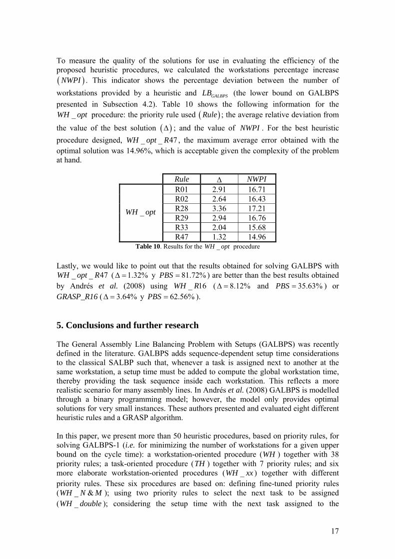
To measure the quality of the solutions for use in evaluating the efficiency of the proposed heuristic procedures, we calculated the workstations percentage increase ( )NWPI . This indicator shows the percentage deviation between the number of workstations provided by a heuristic and GALBPSLB (the lower bound on GALBPS presented in Subsection 4.2). Table 10 shows the following information for the

_WH opt procedure: the priority rule used ( )Rule ; the average relative deviation from

the value of the best solution ( )∆ ; and the value of NWPI . For the best heuristic procedure designed, _ _ 47WH opt R , the maximum average error obtained with the optimal solution was 14.96%, which is acceptable given the complexity of the problem at hand.

Rule ∆ NWPI R01 2.91 16.71 R02 2.64 16.43 R28 3.36 17.21 R29 2.94 16.76 R33 2.04 15.68

_WH opt

R47 1.32 14.96 Table 10. Results for the _WH opt procedure

Lastly, we would like to point out that the results obtained for solving GALBPS with

_ _ 47WH opt R ( 1.32%∆ = y 81.72%PBS = ) are better than the best results obtained by Andrés et al. (2008) using _ 16WH R ( 8.12%∆ = and 35.63%PBS = ) or GRASP_R16 ( 3.64%∆ = y 62.56%PBS = ). 5. Conclusions and further research The General Assembly Line Balancing Problem with Setups (GALBPS) was recently defined in the literature. GALBPS adds sequence-dependent setup time considerations to the classical SALBP such that, whenever a task is assigned next to another at the same workstation, a setup time must be added to compute the global workstation time, thereby providing the task sequence inside each workstation. This reflects a more realistic scenario for many assembly lines. In Andrés et al. (2008) GALBPS is modelled through a binary programming model; however, the model only provides optimal solutions for very small instances. These authors presented and evaluated eight different heuristic rules and a GRASP algorithm. In this paper, we present more than 50 heuristic procedures, based on priority rules, for solving GALBPS-1 (i.e. for minimizing the number of workstations for a given upper bound on the cycle time): a workstation-oriented procedure (WH ) together with 38 priority rules; a task-oriented procedure (TH ) together with 7 priority rules; and six more elaborate workstation-oriented procedures ( _WH xx ) together with different priority rules. These six procedures are based on: defining fine-tuned priority rules ( _ &WH N M ); using two priority rules to select the next task to be assigned ( _WH double ); considering the setup time with the next task assigned to the

18

workstation that is being completed ( _WH lf ); considering all of the positions at which a candidate task can be assigned (Subsection _WH pos ); and performing a local optimization of the tasks assigned to a workstation, either once the workstation is considered to be closable ( _WH swap ) or every time a new task is assigned there ( _WH opt ). We tested the proposed heuristic procedures with a set of self-made instances, and found that the new _WH opt procedure with priority rule R47 ( _ _ 47WH opt R ) yields better results than those published to date for solving GALBPS. Our future work will focus on the design of other metaheuristic procedures for the problem. 6. Acknowledgments The authors are very grateful to Professor Albert Corominas (Technical University of Catalonia) for his valuable comments which have helped to enhance this paper. 7. References Agnetis, A., Arbib, C. (1997), Concurrent operations assignment and sequencing for

particular assembly problems in flow lines. Annals of Operations Research 69, 1–31.

Ağpak, K., Gökçen, H. (2005). Assembly line balancing: Two resource constrained cases. International Journal of Production Economics 96(1), 129–140.

Allahverdi A., Gupta J.N.D. and Aldowaisan T. (1999), A review of scheduling research involving setup considerations. Omega 27, 219–239.

Allahverdi, A., Ng, C.T., Cheng, T.C.E., Kovalyov, M.Y. (2008), A survey of scheduling problems with setup times or costs. European Journal of Operational Research 187, 985-1032.

Andrés, C., Miralles, C., Pastor, R. (2008), Balancing and scheduling tasks in assembly lines with sequence-dependent setup times. European Journal of Operational Research 187, 1212-1223.

Anjos, M.F., Cheng, R.C.H., Currie, C.S.M. (2004), Maximizing revenue in the airline industry under one-way pricing. Journal of the Operational Research Society 55, 535–541.

Amen, M. (2006), Cost-oriented assembly line balancing: Model formulations, solution difficulty, upper and lower bounds. European Journal of Operational Research 168, 747–770.

Arcus, A.L. (1963), An analysis of a computer method of sequencing assembly line operations. Ph.D. dissertation, University of California, Berkeley.

Arcus, A.L. (1966), COMSOAL: A computer method of sequencing operations for assembly lines. International Journal of Production Research 4, 259–277.

Bhattacharjee, T.K., Sahu, S. (1988), A heuristic approach to general assembly line balancing. International Journal of Operations and Production Management 8, 67–77.

19

Bautista, J., Pereira, J. (2002), Ant algorithms for assembly line balancing. Lecture Notes in Computer Science 2463, 65–75.

Baybars, I. (1986), A survey of exact algorithms for the simple assembly line balancing problem, Management Science 32, 909–932.

Becker, C., Scholl, A. (2006), A survey on problems and methods in generalized assembly line balancing. European Journal of Operational Research 168, 694–715.

Boctor, F.F. (1995), A multiple-rule heuristic for assembly line balancing. Journal of the Operational Research Society 46, 62–69.

Boysen, N., Fliedner, M., Scholl, A. (2007), A classification of assembly line balancing problems. European Journal of Operational Research 183, 674–693.

Capacho, L., Pastor, R. (2007), ASALBP: the Alternative Subgraphs Assembly Line Balancing Problem. International Journal of Production Research (first published on 09 April 2007, doi:10.1080/00207540701197010).

Chelouah, R., Siarry, P. (2005), A hybrid method combining continuous tabu search and Nelder-Mead simplex algorithms for the global minimization of multiminima functions. European Journal of Operational Research 161, 636–654.

Corominas, A. (2005), Empirically Adjusted Greedy Algorithms (EAGH): A new approach to solving combinatorial optimisation problems. Working paper IOC-DT-P-2005-22. Universidad Politécnica de Cataluña. Barcelona.

Corominas, A., Pastor, R., Plans, J. (2006), Balancing assembly line with skilled and unskilled workers. OMEGA (in press, corrected proof, available online 9 May 2006, doi: 10.1016/j.omega.2006.03.003).

Erel, E., Sarin, S. (1998), A survey of the assembly line balancing procedures. Production Planning and Control 9, 414–434.

Feo, T.A., Resende, M.G. (1995), Greedy randomized adaptative search procedures. Journal of Global Optimization 6, 109–133.

Gamberini, R., Grassi, A., Rimini, B. (2006), A new multi-objective heuristic algorithm for solving the stochastic assembly line re-balancing problem. International Journal of Production Economics 102, 226–243.

Ghosh, S., Gagnon R.J. (1989), A comprehensive literature review and analysis of the design, balancing and scheduling of assembly systems. International Journal of Production Research 27, 637–670.

Gökçen, H., Ağpak, K., Benzer, R. (2006), Balancing of parallel assembly lines. International Journal of Production Economics 103(2), 600–609.

Graves, S.C., Lamar, B.W. (1983), An Integer Programming Procedure for Assembly System Design Problems. Operations Research 31, 522–545.

Helgeson, W.B., Birnie, D.P. (1961), Assembly line balancing using the ranked positional weight technique. Journal of Industrial Engineering 12, 394–398.

Kao, E.P.C., Queyranne, M. (1982), On dynamic programming methods for assembly line balancing. Operations Research 30, 375–390.

Lagarias, J.C., Reeds, J.A., Wright, M.H., Wright, P.E. (1998), Convergence properties of the Nelder-Mead simplex method in low dimensions. SIAM Journal on Optimization 9, 112–147.

Merengo F. Nava A. Pozzetti (1999), Balancing and sequencing manual mixed model assembly lines. International Journal of Production Research 37(12), 2835–2860.

Miltenburg, J. (2001), U-shaped production lines: a review of theory and practice. International Journal of Production Economics 70(3), 201–214.

Moodie, C.L., Young, H.H. (1965), A heuristic method of assembly line balancing for assumptions of constant or variable work element times. Journal of Industrial Engineering 16, 23–29.

20

Nelder, J.A., Mead, R. (1965), A simplex method for function minimization. The Computer Journal 7, 308–313.

Park, K., Park, S., Kim, W. (1997), A heuristic for an assembly line balancing problem with incompatibility, range, and partial precedence constraints. Computers & Industrial Engineering 32, 321–332.

Pastor, R., Andrés, C., Duran, A., Pérez, M. (2002), Tabu search algorithms for an industrial multi-product and multi-objective assembly line balancing problem, with reduction of the tasks dispersion. Journal of the Operational Research Society 53, 1317–1323.

Ponnambalam, S.G., Aravindan, P., Mogileeswar, G. (1999), A comparative evaluation of assembly line balancing heuristics. International Journal of Advanced Manufacturing Technology 15, 577–586.

Rekiek, B., Dolgui, A., Delchambre, A., Bratcu, A. (2002), State of art of optimization methods for assembly line design, Annual Reviews in Control 26, 163–174.

Sawik, T. (2002), Balancing and scheduling of surface mount technology lines. International Journal of Production Research 40(9), 1973–1991.

Scholl, A. (1999), Balancing and sequencing of assembly lines. Physica-Verlag Heidelberg: Germany. 2nd edition.

Scholl, A., Becker, C. (2006), State-of-the-art exact and heuristic solution procedures for simple assembly line balancing. European Journal of Operational Research 168, 666–693.

Scholl, A., Boysen, N., Fliedner, M. (2006), The sequence-dependent assembly line balancing problem. OR Spectrum (online first 17 November 2006, doi: 10.1007/s00291-006-0070-3).

Scholl, A., Voß, S. (1996), Simple assembly line balancing-Heuristic approaches. Journal of Heuristics 2, 217–244.

Scholl, A., Klein, R. (1997), SALOME: a bidirectional branch and bound procedure for assembly line balancing. Informs Journal on Computing 9, 319–334.

Talbot, F.B., Patterson, J.H. (1984), An integer programming algorithm with network cuts for solving the assembly line balancing problem. Management Science 30, 85–99.

Talbot, F., Patterson, J.H., Gehrlein, W.V. (1986), A comparative evaluation of heuristic line balancing techniques. Management Science 32, 431–453.

Tonge, F.M. (1961), A heuristic program for assembly line balancing. Prentice-Hall. Englewood Cliffs, NJ.

Wee, T.S., Magazine, M.J. (1982), Assembly line balancing as generalized bin packing. Operations Research Letters 1, 56–58.

Wilhelm, W.E. (1999), A column-generation approach for the assembly system design problem with tool changes. International Journal of Flexible Manufacturing Systems 11, 177–205.