U.P.B. Sci. Bull., Series D, Vol. 77, Iss. 3, 2015 ISSN 1454-2358

GLOBAL KINEMATICS CHARACTERISTICS ANALYSIS OF PLANAR MECHANISMS

Guoying ZENG1,Dengfeng ZHAO2, Yubin LU3

Based on the singularity of constraint equations, the analysis method of global kinematics characteristics of planar single-loop mechanisms was studied by using singularity division of the dimension space and the solution space of mechanisms. Results show that this analysis method has two advantages, viz. all global kinematics characteristics are included in the division results and various global analysis problems can be translated into multifarious retrievals of condition-value of vertexes. Thus, this method is appropriate for analysis of complicated mechanisms by computers.

Keywords: planar mechanisms; singularity; solution space; global characteristics

1. Introduction Traditional mechanisms analysis is to solve variation with time about

kinematic parameters, under the condition that links connection relationship, links size and drive condition have been determined. Whereas, global analysis of mechanism motility performance is to discuss mechanisms performance distribution and its evolution process with links size. Traditional mechanisms analysis is based on the kinematics and dynamics, whose analysis method is already quite mature. Many software applications can solve very complicated problems. Global analysis is based on modern mathematics theories such as topology, singular bifurcation theory, group theory and so on.

The global characteristics of mechanisms were closely related with the singularity of mechanisms. However, the current researches only focus on singularity of mechanisms. In the early time, Ting et al. [1] studied the rotatability law for N-bar kinematic chains by a traditional method. Afterwards the researches on the singularity of mechanisms are widely conducted. Alici [2] focused on the determination of singularity contours for a manipulator. Jiang et al. [3] gave the singularity orientation of the Gough–Stewart platform. Hang et al. [4] presented the decoupling conditions of spherical parallel mechanisms. Wolf et al. [5] analyzed the singularities of a three degree of freedom spatial Cassino Parallel manipulators. Li et al.[6] performed a recursive matrix approach in kinematics and dynamics modelling of parallel mechanisms. Researches on the relations between the global kinematics characteristics and the singularity of mechanisms

1 Prof, Southwest University of Science and Technology, PR China, e-mail: zgywf@163.com 2 Prof, Southwest University of Science and Technology, PR China, e-mail: 1264879506 @qq.com 3 Prof, Southwest University of Science and Technology, PR China, e-mail: 289232944 @qq.com

4 Guoying Zeng, Dengfeng Zhao, Yubin Lu

are few. Gao et al. [7] introduce the concept of solution space to the mechanisms evolution analysis, the workspace atlas of parallel planar manipulators were obtained. Zhao et al. [8, 9] using the convex hull division method explored the classification method of single-loop planar and spherical mechanisms.

If viewed from mathematical, mechanisms can be looked as nonlinear geometric constraint equations defined on variables of motion space and dimension space. Variables of motion space here changes with time, such as motion parameter of motion pair. Variables of dimension space here remain constant during movement, such as the size of links. Solution set of constraint equations in motion space is termed as the solution space. Dimension of the solution space is the difference between the amount of motion parameter and the number of constraint equation, which also is the degree of freedom of the mechanism. All characteristics of mechanism depend on the characteristics of the constraint equations, and completely reflected in the solution space. The global analysis of mechanism should include the following two main parts.

(1) The classification of complicated mechanisms For the mechanisms with fixed connection relationship, the topology of

the solution space may mutate with the change of links size. The global structure of all mechanism performance will mutate with the topology mutations of solution space. Thus most natural classification of dimension is formed. Division of high-dimensional dimension space used by all the conditions of classification would generate multitudinous geometric objects (simple or complex). The relationship of geometric objects helps us to grasp overall evolution of the mechanisms types.

(2) The analysis of solution space of the complicated mechanisms The solution space of mechanism with fixed connection relationship and

sizes is determined. To find out the overall structure of the solution space, a straightforward method is that the solution space is divided into geometric objects with simple topologic structure. The boundary of geometric objects is corresponding to the singular motion position. The characteristic of mechanisms is no singular monotonic variation in each geometric object. The adjacency relationship of geometric objects may reveal the whole distribution of mechanisms motion performance.

The global performance analysis problem of general mechanism is complex. In this paper, the global performance analysis about the simplest mechanisms, that is planar single loop mechanism, is only discussed. The analysis conclusions are given for 4,5,6-link mechanisms.

2. Constraint equations and singularity of mechanisms

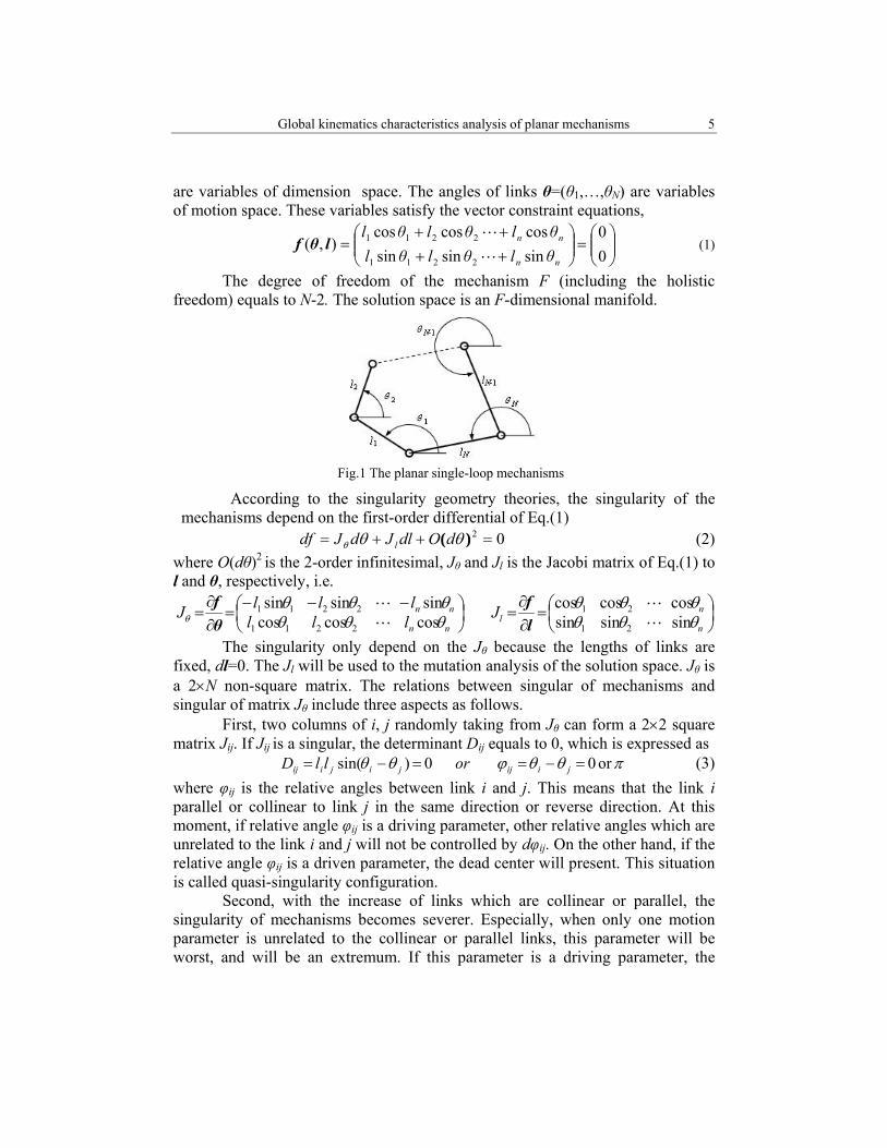
A single-loop N-link planar mechanism is shown in Fig.1, where N links are connected with N revolute joints. The lengths of links are l=(l1,…,lN), which

Global kinematics characteristics analysis of planar mechanisms 5

are variables of dimension space. The angles of links θ=(θ1,…,θN) are variables of motion space. These variables satisfy the vector constraint equations,

⎟⎟⎠

⎞⎜⎜⎝

⎛=⎟⎟

⎠

⎞⎜⎜⎝

⎛++++

=00

sinsinsincoscoscos

),(2211

2211

nn

nn

θlθlθlθlθlθl

lθf (1)

The degree of freedom of the mechanism F (including the holistic freedom) equals to N-2. The solution space is an F-dimensional manifold.

Fig.1 The planar single-loop mechanisms

According to the singularity geometry theories, the singularity of the mechanisms depend on the first-order differential of Eq.(1)

02 =++= )( θθθ dOdlJdJdf l (2) where O(dθ)2

is the 2-order infinitesimal, Jθ and Jl is the Jacobi matrix of Eq.(1) to l and θ, respectively, i.e.

⎟⎠⎞

⎜⎝⎛=

∂∂

=⎟⎠⎞

⎜⎝⎛ −−−=

∂∂

=n

nl

nn

nn JllllllJ θθθ

θθθθθθθθθ

θ sinsinsincoscoscos

coscoscossinsinsin

21

21

2211

2211

lf

θf

The singularity only depend on the Jθ because the lengths of links are fixed, dl=0. The Jl will be used to the mutation analysis of the solution space. Jθ is a 2×N non-square matrix. The relations between singular of mechanisms and singular of matrix Jθ include three aspects as follows.

First, two columns of i, j randomly taking from Jθ can form a 2×2 square matrix Jij. If Jij is a singular, the determinant Dij equals to 0, which is expressed as

πθθϕθθ or 0 0)sin( =−==−= jiijjijiij orllD (3) where φij is the relative angles between link i and j. This means that the link i parallel or collinear to link j in the same direction or reverse direction. At this moment, if relative angle φij is a driving parameter, other relative angles which are unrelated to the link i and j will not be controlled by dφij. On the other hand, if the relative angle φij is a driven parameter, the dead center will present. This situation is called quasi-singularity configuration.

Second, with the increase of links which are collinear or parallel, the singularity of mechanisms becomes severer. Especially, when only one motion parameter is unrelated to the collinear or parallel links, this parameter will be worst, and will be an extremum. If this parameter is a driving parameter, the

6 Guoying Zeng, Dengfeng Zhao, Yubin Lu

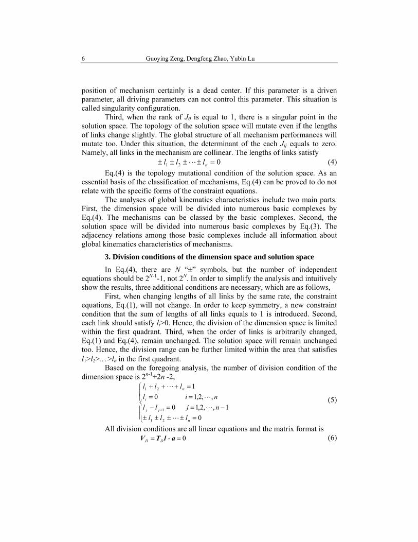
position of mechanism certainly is a dead center. If this parameter is a driven parameter, all driving parameters can not control this parameter. This situation is called singularity configuration.

Third, when the rank of Jθ is equal to 1, there is a singular point in the solution space. The topology of the solution space will mutate even if the lengths of links change slightly. The global structure of all mechanism performances will mutate too. Under this situation, the determinant of the each Jij equals to zero. Namely, all links in the mechanism are collinear. The lengths of links satisfy

021 =±±±± nlll (4) Eq.(4) is the topology mutational condition of the solution space. As an

essential basis of the classification of mechanisms, Eq.(4) can be proved to do not relate with the specific forms of the constraint equations.

The analyses of global kinematics characteristics include two main parts. First, the dimension space will be divided into numerous basic complexes by Eq.(4). The mechanisms can be classed by the basic complexes. Second, the solution space will be divided into numerous basic complexes by Eq.(3). The adjacency relations among those basic complexes include all information about global kinematics characteristics of mechanisms.

3. Division conditions of the dimension space and solution space

In Eq.(4), there are N “±” symbols, but the number of independent equations should be 2N-1-1, not 2N. In order to simplify the analysis and intuitively show the results, three additional conditions are necessary, which are as follows,

First, when changing lengths of all links by the same rate, the constraint equations, Eq.(1), will not change. In order to keep symmetry, a new constraint condition that the sum of lengths of all links equals to 1 is introduced. Second, each link should satisfy li>0. Hence, the division of the dimension space is limited within the first quadrant. Third, when the order of links is arbitrarily changed, Eq.(1) and Eq.(4), remain unchanged. The solution space will remain unchanged too. Hence, the division range can be further limited within the area that satisfies l1>l2>…>ln in the first quadrant.

Based on the foregoing analysis, the number of division condition of the dimension space is 2n-1+2n -2,

⎪⎪⎩

⎪⎪⎨

⎧

=±±±±−==−

===+++

+

01,,2,1 0

,,2,1 01

21

1

21

n

jj

i

n

lllnjllnil

lll

(5)

All division conditions are all linear equations and the matrix format is 0- == alTV DD (6)

Global kinematics characteristics analysis of planar mechanisms 7

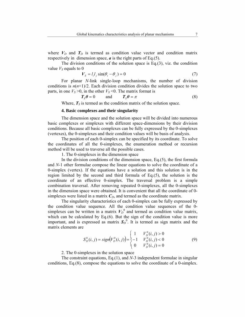
where VD and TD is termed as condition value vector and condition matrix respectively in dimension space, a is the right parts of Eq.(5).

The division conditions of the solution space is Eq.(3), viz. the condition value VS equals to 0

0)sin( =−= jijiS ll θθV (7) For planar N-link single-loop mechanisms, the number of division

conditions is n(n+1)/2. Each division condition divides the solution space to two parts, in one VS >0, in the other VS <0. The matrix format is

π== θTθT SS and0 (8) Where, TS is termed as the condition matrix of the solution space.

4. Basic complexes and their singularity

The dimension space and the solution space will be divided into numerous basic complexes or simplexes with different space-dimensions by their division conditions. Because all basic complexes can be fully expressed by the 0-simplexes (vertexes), the 0-simplexes and their condition values will be basis of analysis.

The position of each 0-simplex can be specified by its coordinate. To solve the coordinates of all the 0-simplexes, the enumeration method or recursion method will be used to traverse all the possible cases.

1. The 0-simplexes in the dimension space In the division conditions of the dimension space, Eq.(5), the first formula

and N-1 other formulae compose the linear equations to solve the coordinate of a 0-simplex (vertex). If the equations have a solution and this solution is in the region limited by the second and third formula of Eq.(5), the solution is the coordinate of an effective 0-simplex. The traversal problem is a simple combination traversal. After removing repeated 0-simplexes, all the 0-simplexes in the dimension space were obtained. It is convenient that all the coordinate of 0-simplexes were listed in a matrix CD, and termed as the coordinate matrix.

The singularity characteristics of each 0-simplex can be fully expressed by the condition value sequence. All the condition value sequences of the 0-simplexes can be written in a matrix VD

0 and termed as condition value matrix, which can be calculated by Eq.(6). But the sign of the condition value is more important, and is expressed as matrix SD

0. It is termed as sign matrix and the matrix elements are

( )⎪⎩

⎪⎨⎧

=<−>

==0),(00),(10),(1

),(),(0

0

0

00

jiVjiVjiV

jiVsignjiSD

D

D

DD (9)

2. The 0-simplexes in the solution space The constraint equations, Eq.(1), and N-3 independent formulae in singular

conditions, Eq.(8), compose the equations to solve the coordinate of a 0-simplex.

8 Guoying Zeng, Dengfeng Zhao, Yubin Lu

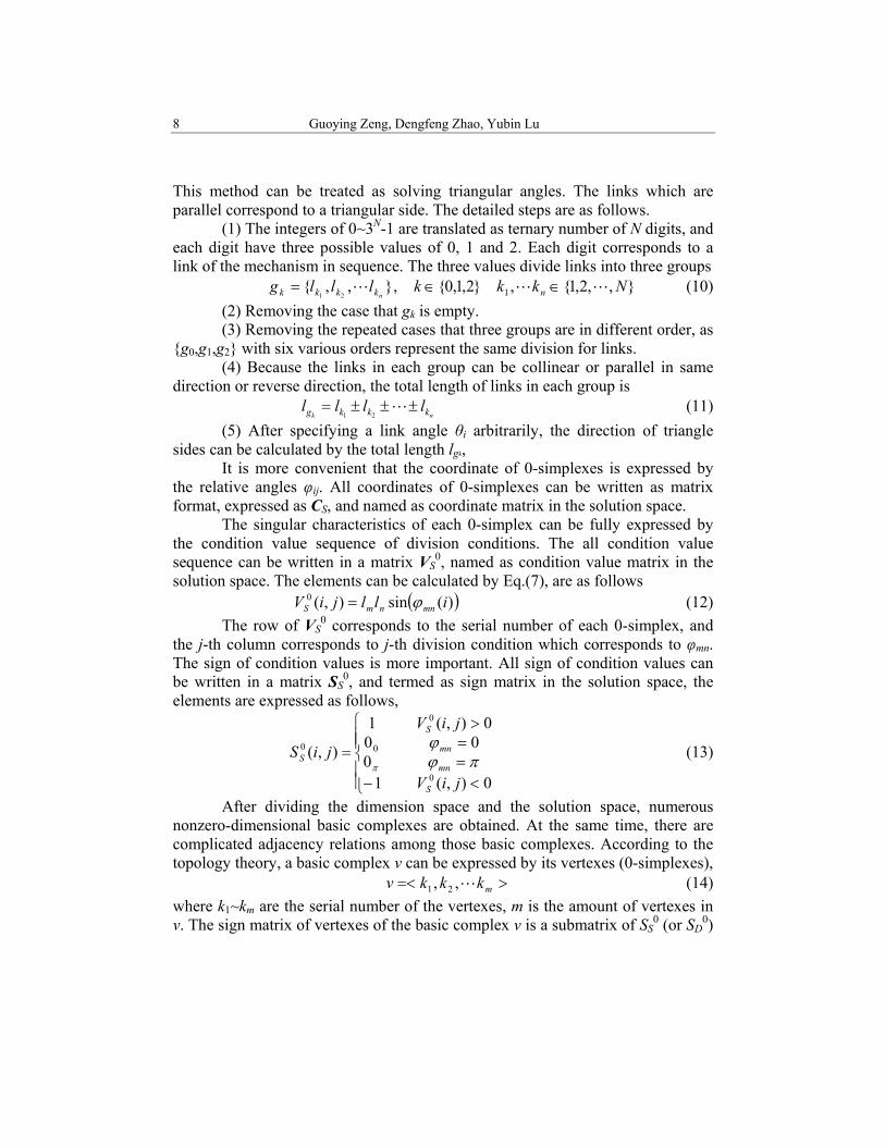
This method can be treated as solving triangular angles. The links which are parallel correspond to a triangular side. The detailed steps are as follows.

(1) The integers of 0~3N-1 are translated as ternary number of N digits, and each digit have three possible values of 0, 1 and 2. Each digit corresponds to a link of the mechanism in sequence. The three values divide links into three groups

},,2,1{,}2,1,0{,},,{ 121Nkkklllg nkkkk n

∈∈= (10) (2) Removing the case that gk is empty. (3) Removing the repeated cases that three groups are in different order, as

{g0,g1,g2} with six various orders represent the same division for links. (4) Because the links in each group can be collinear or parallel in same

direction or reverse direction, the total length of links in each group is nk kkkg llll ±±±=

21 (11)

(5) After specifying a link angle θi arbitrarily, the direction of triangle sides can be calculated by the total length lgk,

It is more convenient that the coordinate of 0-simplexes is expressed by the relative angles φij. All coordinates of 0-simplexes can be written as matrix format, expressed as CS, and named as coordinate matrix in the solution space.

The singular characteristics of each 0-simplex can be fully expressed by the condition value sequence of division conditions. The all condition value sequence can be written in a matrix VS

0, named as condition value matrix in the solution space. The elements can be calculated by Eq.(7), are as follows

( ))(sin),(0 illjiV mnnmS ϕ= (12) The row of VS

0 corresponds to the serial number of each 0-simplex, and the j-th column corresponds to j-th division condition which corresponds to φmn. The sign of condition values is more important. All sign of condition values can be written in a matrix SS

0, and termed as sign matrix in the solution space, the elements are expressed as follows,

⎪⎪⎩

⎪⎪⎨

⎧

<−==>

=

0),(10

000),(1

),(0

0

0

0

jiV

jiV

jiS

S

mn

mn

S

S πϕϕ

π (13)

After dividing the dimension space and the solution space, numerous nonzero-dimensional basic complexes are obtained. At the same time, there are complicated adjacency relations among those basic complexes. According to the topology theory, a basic complex v can be expressed by its vertexes (0-simplexes),

>=< mkkkv ,, 21 (14) where k1~km are the serial number of the vertexes, m is the amount of vertexes in v. The sign matrix of vertexes of the basic complex v is a submatrix of SS

0 (or SD0)

Global kinematics characteristics analysis of planar mechanisms 9

and be expressed as Sv0. The singularly and adjacency relations of all the basic

complexes can be obtained from sign matrix SS0 (or SD

0). 1. The analysis principle of nonzero-complexes (1) For the sign matrix Sv

0 of a basic complex v, there are not the elements with inverse sign. Hence, the all interior points have same sign and which can be calculated from the Sv

0 as follows

⎥⎦

⎤⎢⎣

⎡= ∑

=

m

iv jiSsignjs

1

0 ),()( (15)

All s(j) compose the sign sequence, Sv, of the basic complex v, which can fully express the singularity characteristics of the basic complex v. In the dimension space (or solution space), sign sequences of all the basic m-complexes can be written in a matrix SD

m (or SSm) and be termed as the sign matrix of basic

m-complexes. (2) Each basic complex can be identified by the sign sequence. (3) For two basic m-complexes with the sign sequences Sv and Sv’, if only

the k-th sign s(k) is reverse to s’(k) and other signs are same, the two basic complexes are adjacent each other. The adjacency boundary is a basic (m-1)-complex whose k-th sign is 0 and other signs are equaled to Sv or Sv’.

(4) For a basic complex v, the dimension of v is Dv, and the dimension of embedment space of v is DS. The 0 elements set of sign sequence Sv is {k1

0,…,kn0}

and those rows of the condition matrix TS (or TD) compose a matrix Tv. Obviously, the matrix Tv is the constraint matrix of v. Those parameters should satisfy

)( vSv TrankDD −= (16) 2. Method of obtaining all the basic nonzero-complexes Any basic complex can be uniquely specified by its sign sequence Sv, so

the enumeration method or recursion method can always traverse all possible cases, and all basic complexes can be obtained.

The traversal problem of a sequence Sv with finite length and finite value is easy. For each case, the analysis steps are as follows.

(1) According to the first and second item of the above section, “the analysis principle of nonzero-simplexes”, for a specified sign sequence Sv, the vertexes of the basic complex v, can be obtained by searching the sign matrix of 0-simplexes SD

0 (or SS0), and the sign matrix of the basic complex, Sv

0,can be obtained at the same time.

(2) According to the fourth item of the above section, “the analysis principle of nonzero-simplexes”, the dimension of the basic complex, Dv, can be calculated by Eq.(16).

(3) The sign matrix, SDm or SS

m can be formed by uniting all sign sequences of basic m-complexes.

10 Guoying Zeng, Dengfeng Zhao, Yubin Lu

For N-link mechanisms, the division results are many basic complexes in the dimension space or the solution space. The adjacency relations among those basic complexes can be fully expressed by the relational matrixes. If there are J basic k-complexes and I basic (k-1)-complexes, the relational matrix Lk is an I by J matrix and the elements are

⎪⎩

⎪⎨⎧

∂∉−∂∈−+∂∈

=

ji

ji

jik

vvvvvv

jiL 0 1

1),( (17)

where vi is a basic (k-1)-complex, vj is a basic k-complex, and ∂vj expresses the boundary of vj.

According to the first or fourth item in the above section, “the analysis principle of nonzero-simplexes”, all relational matrixes can be obtained.

5. Analysis of mechanisms global characteristics for typical problems

The analysis of mechanisms global characteristics is very comprehensive. In this paper, only three general problems are discussed and the 4, 5, 6-link mechanisms were given.

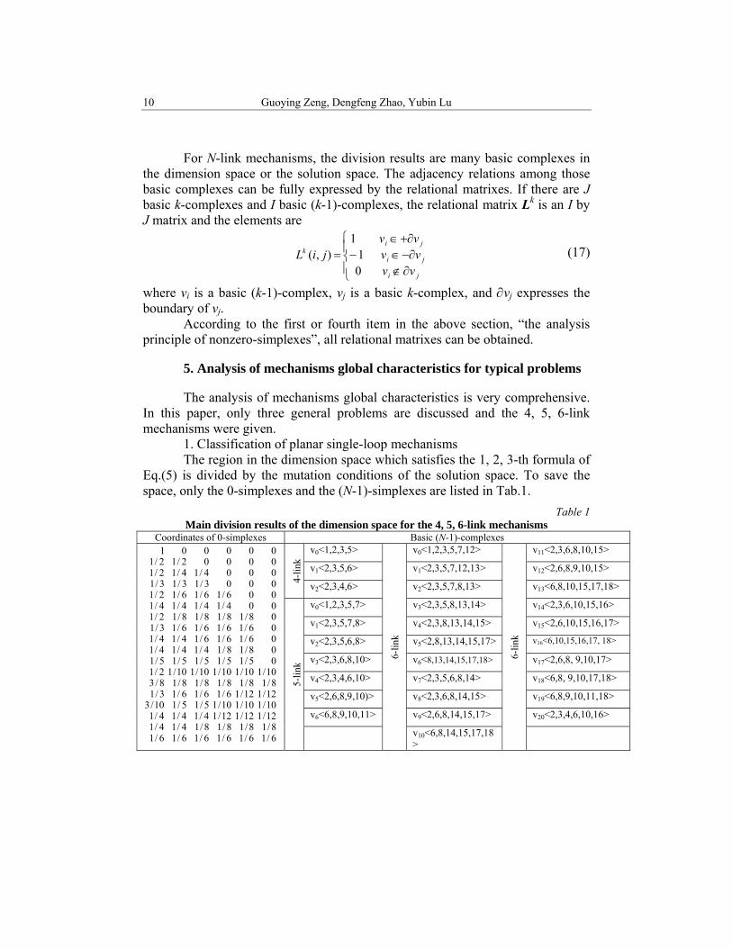
1. Classification of planar single-loop mechanisms The region in the dimension space which satisfies the 1, 2, 3-th formula of

Eq.(5) is divided by the mutation conditions of the solution space. To save the space, only the 0-simplexes and the (N-1)-simplexes are listed in Tab.1.

Table 1 Main division results of the dimension space for the 4, 5, 6-link mechanisms

Coordinates of 0-simplexes Basic (N-1)-complexes

6/16/16/16/16/16/18/18/18/18/14/14/1

12/112/112/14/14/14/110/110/110/15/15/110/312/112/16/16/16/13/1

8/18/18/18/18/18/310/110/110/110/110/12/1

05/15/15/15/15/108/18/14/14/14/106/16/16/14/14/106/16/16/16/13/108/18/18/18/12/1004/14/14/14/1006/16/16/12/10003/13/13/10004/14/12/100002/12/1000001

4-lin

k

v0<1,2,3,5>

6-lin

k

v0<1,2,3,5,7,12>

6-lin

k

v11<2,3,6,8,10,15>

v1<2,3,5,6> v1<2,3,5,7,12,13> v12<2,6,8,9,10,15>

v2<2,3,4,6> v2<2,3,5,7,8,13> v13<6,8,10,15,17,18>

5-lin

k

v0<1,2,3,5,7> v3<2,3,5,8,13,14> v14<2,3,6,10,15,16>

v1<2,3,5,7,8> v4<2,3,8,13,14,15> v15<2,6,10,15,16,17>

v2<2,3,5,6,8> v5<2,8,13,14,15,17> v16<6,10,15,16,17, 18>

v3<2,3,6,8,10> v6<8,13,14,15,17,18> v17<2,6,8, 9,10,17>

v4<2,3,4,6,10> v7<2,3,5,6,8,14> v18<6,8, 9,10,17,18>

v5<2,6,8,9,10)> v8<2,3,6,8,14,15> v19<6,8,9,10,11,18>

v6<6,8,9,10,11> v9<2,6,8,14,15,17> v20<2,3,4,6,10,16>

v10<6,8,14,15,17,18>

Global kinematics characteristics analysis of planar mechanisms 11

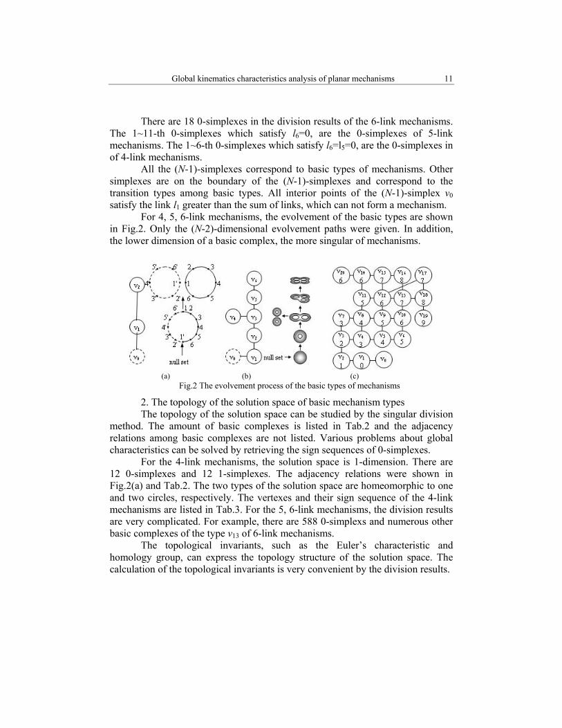
There are 18 0-simplexes in the division results of the 6-link mechanisms. The 1~11-th 0-simplexes which satisfy l6=0, are the 0-simplexes of 5-link mechanisms. The 1~6-th 0-simplexes which satisfy l6=l5=0, are the 0-simplexes in of 4-link mechanisms.

All the (N-1)-simplexes correspond to basic types of mechanisms. Other simplexes are on the boundary of the (N-1)-simplexes and correspond to the transition types among basic types. All interior points of the (N-1)-simplex v0 satisfy the link l1 greater than the sum of links, which can not form a mechanism.

For 4, 5, 6-link mechanisms, the evolvement of the basic types are shown in Fig.2. Only the (N-2)-dimensional evolvement paths were given. In addition, the lower dimension of a basic complex, the more singular of mechanisms.

(a) (b) (c)

Fig.2 The evolvement process of the basic types of mechanisms

2. The topology of the solution space of basic mechanism types The topology of the solution space can be studied by the singular division

method. The amount of basic complexes is listed in Tab.2 and the adjacency relations among basic complexes are not listed. Various problems about global characteristics can be solved by retrieving the sign sequences of 0-simplexes.

For the 4-link mechanisms, the solution space is 1-dimension. There are 12 0-simplexes and 12 1-simplexes. The adjacency relations were shown in Fig.2(a) and Tab.2. The two types of the solution space are homeomorphic to one and two circles, respectively. The vertexes and their sign sequence of the 4-link mechanisms are listed in Tab.3. For the 5, 6-link mechanisms, the division results are very complicated. For example, there are 588 0-simplexs and numerous other basic complexes of the type v13 of 6-link mechanisms.

The topological invariants, such as the Euler’s characteristic and homology group, can express the topology structure of the solution space. The calculation of the topological invariants is very convenient by the division results.

12 Guoying Zeng, Dengfeng Zhao, Yubin Lu

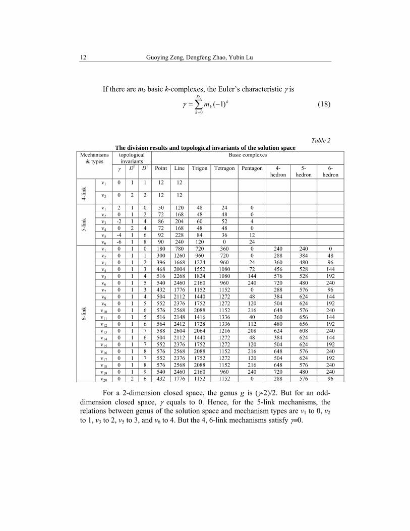
If there are mk basic k-complexes, the Euler’s characteristic γ is

∑=

−=sD

k

kkm

0)1(γ (18)

Table 2 The division results and topological invariants of the solution space

Mechanisms & types

topological invariants

Basic complexes

γ D0 D1 Point Line Trigon Tetragon Pentagon 4- hedron

5-hedron

6- hedron

4-lin

k

v1 0 1 1 12 12

v2 0 2 2 12 12

5-lin

k

v1 2 1 0 50 120 48 24 0 v2 0 1 2 72 168 48 48 0 v3 -2 1 4 86 204 60 52 4 v4 0 2 4 72 168 48 48 0 v5 -4 1 6 92 228 84 36 12 v6 -6 1 8 90 240 120 0 24

6-lin

k

v1 0 1 0 180 780 720 360 0 240 240 0 v2 0 1 1 300 1260 960 720 0 288 384 48v3 0 1 2 396 1668 1224 960 24 360 480 96 v4 0 1 3 468 2004 1552 1080 72 456 528 144 v5 0 1 4 516 2268 1824 1080 144 576 528 192 v6 0 1 5 540 2460 2160 960 240 720 480 240 v7 0 1 3 432 1776 1152 1152 0 288 576 96 v8 0 1 4 504 2112 1440 1272 48 384 624 144 v9 0 1 5 552 2376 1752 1272 120 504 624 192 v10 0 1 6 576 2568 2088 1152 216 648 576 240 v11 0 1 5 516 2148 1416 1336 40 360 656 144 v12 0 1 6 564 2412 1728 1336 112 480 656 192 v13 0 1 7 588 2604 2064 1216 208 624 608 240 v14 0 1 6 504 2112 1440 1272 48 384 624 144 v15 0 1 7 552 2376 1752 1272 120 504 624 192 v16 0 1 8 576 2568 2088 1152 216 648 576 240 v17 0 1 7 552 2376 1752 1272 120 504 624 192 v18 0 1 8 576 2568 2088 1152 216 648 576 240 v19 0 1 9 540 2460 2160 960 240 720 480 240 v20 0 2 6 432 1776 1152 1152 0 288 576 96

For a 2-dimension closed space, the genus g is (γ-2)/2. But for an odd-dimension closed space, γ equals to 0. Hence, for the 5-link mechanisms, the relations between genus of the solution space and mechanism types are v1 to 0, v2 to 1, v3 to 2, v5 to 3, and v6 to 4. But the 4, 6-link mechanisms satisfy γ≡0.

Global kinematics characteristics analysis of planar mechanisms 13

Table 3 3 All the 0-simplexes and their sign sequences of the 4-link mechanisms

Type v1 Type v2 1 1’ 2 2’ 3 3’ 4 4’ 5 5’ 6 6’ 1 1’ 2 2’ 3 3’ 4 4’ 5 5’ 6 6’

φ12 0π 0π -1 1 -1 1 -1 1 -1 1 -1 1 -1 1 -1 1 -1 1 -1 1 -1 1 -1 1 φ13 -1 1 0π 0π -1 1 1 -1 1 -1 1 -1 1 -1 1 -1 1 -1 1 -1 1 -1 1 -1 φ14 1 -1 1 -1 1 -1 0π 0π -1 1 1 -1 0π 0π 00 00 1 -1 -1 1 -1 1 1 -1 φ23 1 -1 -1 1 00 00 -1 1 -1 1 -1 1 -1 1 -1 1 -1 1 -1 1 -1 1 -1 1 φ24 -1 1 -1 1 -1 1 -1 1 00 00 -1 1 -1 1 1 -1 0π 0π 00 00 1 -1 -1 1 φ34 -1 1 -1 1 -1 1 1 -1 1 -1 00 00 1 -1 -1 1 -1 1 1 -1 0π 0π 00 00

For a solution space G and the integer group Z, the k-dimensional homology group is expressed as Hk(G,Z) and its dimension Dk is

)()( 1+−−= kkk

k LrankLrankmD (19) where rank(Lk) is the rank of the relational matrix Lk. For an m-dimensional solution space, there are m+1 homology groups. But their dimension satisfy Dk=Dm-k, so only the D1 and D0 are listed in Tab.2. The D0 is number of connected branches and the D1 corresponds to the genus. The types of mechanisms that the number of connected branches is equal to 2 include the v2 of 4-link, v4 of 5-link and v20 of 6-link mechanism. For 6-link mechanisms, genus of the solution space increases 1 at each evolvement.

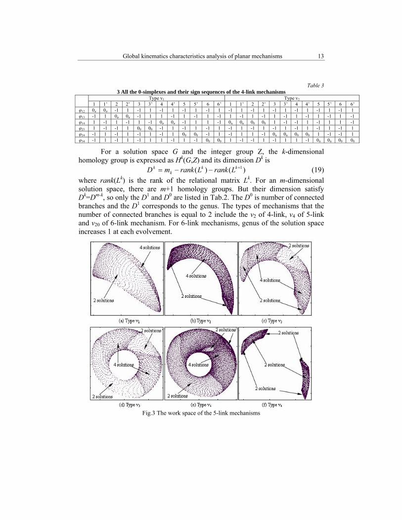
Fig.3 The work space of the 5-link mechanisms

14 Guoying Zeng, Dengfeng Zhao, Yubin Lu

The work space of a mechanism can be treated as the projection of the solution space on the physics space. For a mechanism with Ns-dimension solution space and Nw-dimension work space, a generic point in work space correspond to a (Ns-Nw)-dimension space. The work space can be divided into many regions by some singularly conditions and the topology is different in different regions.

For a 5-link mechanism, typical work space is shown in Fig.3. The topology of solution space of the 6 types of mechanisms can be clearly observed from the work space. The work space is divided into several regions. The number of solutions is different in different regions. There are two types of regions, two solutions and four solutions. For example, the 4-link mechanisms have three types of the work spaces, . Deep discussion can be referenced in Ref. [9].

3. Rotatability analysis of the mechanisms The rotatability analysis of a mechanism is to ascertain whether a relative

angle φij (or combination of relative angles) can fully rotate. A relative angle which can fully rotate be termed as full-angle. After division, rotatability analysis can be completed by retrieving the sign matrix SS

0. For a φij, if the sign 00 and 0π are included simultaneously in the signs of all 0-simplexes, the φij is a full angle.

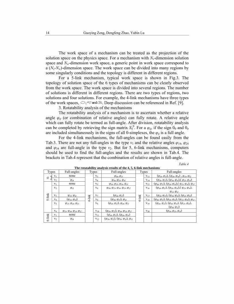
For the 4-link mechanisms, the full-angles can be found easily from the Tab.3. There are not any full-angles in the type v1 and the relative angles φ14, φ24 and φ34 are full-angle in the type v2. But for 5, 6-link mechanisms, computers should be used to find the full-angles and the results are shown in Tab.4. The brackets in Tab.4 represent that the combination of relative angles is full-angle.

Table 4 The rotatability analysis results of the 4, 5, 6-link mechanisms

Types Full-angles Types Full-angles Types Full-angles

4- link v1 none

6-ln

k

v3 φi6, φi5

6-in

k

v13 (φi6, φi5), (φi6, φi4) , φi3, φi2 v2 φi4 v4 φi6, φi5, φi4 v14 (φi6, φi5), (φi6, φi4),( φi5, φi4)

5-lin

k

v1 none v5 φi6, φi5, φi4, φi3 v15 (φi6, φi5), (φi6, φi4),( φi5, φi4), φi3 v2 φi5 v6 φi6, φi5, φi4, φi3, φi2 v16 (φi6, φi5), (φi6, φi4),( φi5, φi4),

φi3, φi2 v3 φi5, φi4 v7 (φi6, φi5) v17 (φi6, φi5), (φi6, φi4), (φi3, φi6) v4 (φi5, φi4) v8 (φi6, φi5), φi4 v18 (φi6, φi5), (φi6, φi4), (φi3, φi6), φi2 v5 φi5, φi4, φi3 v9 (φi6, φi5), φi4, φi3 v19 (φi6, φi5), (φi6, φi4), (φi3, φi6),

(φi6, φi2) v6 φi5, φi4, φi3, φi2 v10 (φi6, φi5), φi4, φi3, φi2 v20 (φi6, φi5, φi4)

6-lin

k v1 none v11 (φi6, φi5), (φi6, φi4) v2 φi6 v12 (φi6, φi5), (φi6, φi4), φi3

Global kinematics characteristics analysis of planar mechanisms 15

In addition, for multi-degree of freedom mechanisms, motion path which evade the singularity configurations can be programmed by retrieving of the condition value sign of 0-simplexes.

6. Conclusions

The analysis method discussed in this paper is mainly consisted of three parts. (1) All the singularity conditions of the planar single-loop mechanisms are obtained from the singularity of constraint equations. (2) The singularity division method is the basic method. (3) The global characteristics analysis is translated into the multifarious retrieval for the sign matrix of 0-simplexes. The analysis method is suitable for computerized analysis on more complex mechanisms.

However, the current study is still inadequate. Further research will be conducting in the following aspects, i.e., popularizing this method to more complicated mechanisms, and developing analysis software concerning the global characteristics of the mechanisms.

Acknowledgment This paper was supported by National Natural Science Foundation of China

(51375410).

R E F E R E N C E S

[1] K.L. Ting and Y.W. Liu, Rotatability laws for N-bar kinematic chains and their proof. ASME Journal of Mechanisms Transmissions and Automation in Design, vol.108,no.1, Jan.1991,pp 32-39

[2] G. Alici, Determination of singularity contours for five-bar planar parallel manipulators. Robotica, vol.18, no. 5, May.2000, pp.569- 575

[3] Q.M. Jiang and C.M. Gosselin, Determination of the maximal singularity-free orientation workspace for the Gough–Stewart platform. Mechanism and Machine Theory, vol.44, no.6, Jun.2009, pp.1281-1293

[4] L.B. Hang and Y. Wang, Study on the decoupling conditions of the spherical parallel mechanism based on the criterion for topologically decoupled parallel mechanisms, Chinese Journal of Mechanical Engineering, vol. 41, no. 9, Sep. 2005, pp.28-32

[5] Alon Wolf, Erika Ottaviano, Moshe Shoham, Marco Ceccarelli, Application of line geometry and linear complex approximation to singularity analysis of the 3-DOF CaPaMan parallel manipulator, Mechanism and Machine Theory, vol.39, no.1, Jan.2004, pp.75-95

[6] Yangmin Li, Stefan Staicu, Inverse dynamics of a 3-PRC parallel kinematic machine, Nonlinear Dynamics, vol.67, no.1, Jan.2012, pp. 1031-1041

16 Guoying Zeng, Dengfeng Zhao, Yubin Lu

[7] F. Gao, X.Q Zhang and Y.S. Zhao, A physical model of the solution space and the atlas of reachable workspace for 2-DOF parallel planar manipulators, Mechanism and Machine Theory vol.31, no.2, Feb. 1996, pp. 173-184

[8] D.F. Zhao, Dimension Classification Method of Planar Mechanism Based on Convex Hull Division, Chinese Journal of Mechanical Engineering , vol.45 , no.4, Apr.2009, pp.100-104

[9] D.F. Zhao, G.Y. Zeng, Y.B. Lu, The classification method of spherical single-loop mechanisms, Mechanism and Machine Theory,vol. 51, no. 5, May.2012, pp.46-57