Uppsala UniversityDepartment of Physics and Astronomy

Division of Theoretical PhysicsDegree Project in Physics 15 HP

Geometrical structures inBlack holes

Author:Roberto Goranci

Supervisor:Giuseppe Dibitetto

Subject reader:Ulf Lindstrom

June 26, 2014

Abstract

We solve the Einstein field equations with a negative cosmological constant (Λ < 0)where the solution gives us topological black holes. Furthermore, we define the surfacegravity’s relation to the black hole temperature and express the mass of the black holes.At the singularity we see that the Euclidean metric possesses a conical structure whichindicates that the black hole is unstable everywhere except the singularity. Using theEuclidean metric to formulate the temperature and the mass of the black holes we cansee that the heat capacity is positive and therefore these black holes are stable.

Sammanfattning

Vi loser Einstein field equations med en negativ kosmologisk konstant (Λ < 0) darlosningarna ger oss topologiska svarta hal. Dessutom kan vi definiera ytgravitationensrelation till svarta halens temperature och formulera massan. Vid singulariteten ser viatt den euklidiska metriken besitter en konisk struktur som indikerar att dessa svarta halar instabila overallt forutom vid singulariteten. Genom att anvanda euklidiska metrikenkan vi definiera temperaturen och massan av dessa svarta hal, som vi sedan kan anvandafor att se att varmekapaciteten ar positiv vilket visar att dessa svarta hal ar stabila.

I

Contents1 Introduction 1

2 Method 2

3 Differential geometry 23.1 Manifolds . . . . . . . . . . . . . . . . . . . . . . . . . . . . . . . . . . . . . . 33.2 Levi-Civita Connection . . . . . . . . . . . . . . . . . . . . . . . . . . . . . . . 43.3 Curvature . . . . . . . . . . . . . . . . . . . . . . . . . . . . . . . . . . . . . . 43.4 Ricci tensor and Ricci scalar . . . . . . . . . . . . . . . . . . . . . . . . . . . . 7

4 General Relativity 74.1 Einstein’s field equations . . . . . . . . . . . . . . . . . . . . . . . . . . . . . . 8

5 Black holes 115.1 Schwarzschild solution . . . . . . . . . . . . . . . . . . . . . . . . . . . . . . . 115.2 Reissner-Nordstrom Solution . . . . . . . . . . . . . . . . . . . . . . . . . . . 155.3 Kerr-Newman solution . . . . . . . . . . . . . . . . . . . . . . . . . . . . . . . 155.4 Black hole thermodynamics . . . . . . . . . . . . . . . . . . . . . . . . . . . . 16

6 Topological black holes 176.1 Geometrical structures . . . . . . . . . . . . . . . . . . . . . . . . . . . . . . . 186.2 Surface gravity and Temperature . . . . . . . . . . . . . . . . . . . . . . . . . 22

7 Discussion 24

Appendices 27

A Schwarzschild solution 27

B Riemann tensors for torus case 28

C Surface gravity 30

D Heat capacity for Schwarzschild metric 31

II

III

1 IntroductionThe theory of General Relativity describes how gravity shapes the spacetime, for examplehow a black hole forms under gravitational force in a region of spacetime. It has had muchsuccess when it comes to experiments and theoretical aspects of General Relativity. For ex-ample, Global positioning system(GPS) is a tool people use to navigate on the earth, whichwould not work if it wasn’t for the General Relativity and its corrections to Special Relativity.General Relativity is still an active research topic in physics. For anyone that is interestedin astrophysics, cosmology, string theory and particle physics.

Black holes were first studied by Pierre-Simon Laplace and John Michell as a thought exper-iment where an object had such strong gravitational fields that not even light could escapeit. The first solution to a black hole came few months after Einstein published his theory ofGeneral Relativity. The person that found the solution was Karl Schwarzschild, who unfor-tunately died two months after he published his results. In his results he found a solution tothe Einstein field equations that described spacetime of a non-rotating massive sphericallysymmetric object. The first real black hole solution where light could not even escape aregion of spacetime was first published 1958 by David Finkelstein. At first black holes wereonly a theoretical object. It wasn’t until the discovery of a pulsar 1967 that studying of grav-itational collapsed compact objects became of interest. In the early 1970 Jacob Beckensteinand Stephen Hawking formulated black hole thermodynamics. Black hole thermodynamicsdescribes the behaviour of a black hole in terms of the laws of thermodynamics by relatingmass to energy, horizon to entropy and surface gravity to temperature. The analogy wascomplete when Stephen Hawking in 1974 by using Quantum Field theory showed that blackholes should radiate like a black body with a temperature proportional to the surface gravityof the black hole. Hawking radiation would only occur if the black hole is warmer than theenvironment surrounding it because the black hole would need to radiate away energy inorder to reach thermal equilibrium. These black hole are hence unstable.

One of the main purposes of studying black holes, is to understand gravity in a betterway. On earth we experience Newtonian gravity where the gravity is very weak, but at blackholes the gravity becomes very strong. So we have to treat the black holes using QuantumMechanics and therefore we have a theory called quantum gravity, which is a theory thattries to combine the other fundamental forces with gravity.

We first consider a vacuum solution to the Einstein field equations where the only contri-bution is the Einstein tensor. By doing so we obtain the Schwarzschild metric as a solutionwhich has singularities at r = 0 and r = rs. Birkhoff’s theorem states that any spheri-cally symmetric solution of the vacuum field equations must be static and asymptoticallyflat1 [1]. No-hair theorem states that all black hole solutions that are asymptotically flat(Λ = 0) can be characterized by only three externally observable classical parameters, i.emass, electric charge and angular momentum. For example the Reissner-Nordstrom metricwhich is a static solution to the Einstein-Maxwell field equations2 which has a charge butis non-rotating i.e the angular momentum is zero. If the black hole was rotating we wouldhave the Kerr-Newman metric.

In order to understand the nature of black holes we have to formulate the black hole ther-modynamics: The zeroth law of black hole thermodynamics suggests that the surface gravityis equivalent to the temperature. The first law of black hole thermodynamics tells us thatthe energy has to be conserved. For black holes to satisfy the second law of black holethermodynamics the black holes need to have entropy. If black holes carried no entropy wewould violate the second law by throwing in mass into the black hole. The third law statesthat the surface gravity cannot be zero3, in other words the entropy of a system at absolutezero is well defined due to being in the ground state. Black hole thermodynamic laws aredifferent from the regular thermodynamic laws because when studying black holes we have

1curvature vanishes at large distances from some regions, i.e the larger the distance the closer the geometrybecome to that of Minkowski spacetime

2Einstein-Maxwell Field equations: the energy-momentum tensor is of an electromagnetic field in freespace i.e the electromagnetic stress-energy tensor

3Extremal black holes have vanishing surface gravity, this is the smallest possible black hole that can exist.

1

to take the energy conditions from General relativity into consideration. Using these blackhole thermodynamic laws we can see that surface gravity of a black hole is related to thetemperature and the area of the event horizon is related with entropy.

In General Relativity it was assumed that black holes formed by gravitational collapse shouldhave a spherical horizon [2]. The Einstein field equations with a cosmological term Λ, admitsolutions to black holes which are asymptotic to either de Sitter (Λ > 0) or anti-de Sitter(Λ < 0) space. Asymptotic means here that we feel the presence of the cosmological constantin the entire universe. Solutions to these Einstein’s field equations (EFE’s) are not forcedto have a spherical horizon and obey thermodynamics laws like the asymptotically flat blackhole [3].

When we study the EFE’s with a negative cosmological constant the no-hair theoremfails because of the violation of the so called weak energy condition, which would imply thatthe Black holes would not need to have a spherical horizon. Instead we could find so-calledtopological black holes.

The aim for this thesis is to make an attempt to understand Black holes with unusualtopology [9]. The metric we consider will yield us three different geometrical shapes: sphere,torus and hyperbolic space. Given a solution to a metric we can find information aboutthe nature of its roots. From this information we can see what solutions are black holeinterpretation and which are not. Using statistical mechanics we can define the mass andthe size of the black hole and the surface gravity which is in itself related to the temperatureof the black hole. We can then explore the quantum effects of these black holes by studyingthe heat capacity.

2 MethodThe references [1] to [8] are mostly books but there are some articles there as well. Thesereferences are used to formulate the differential geometry and General Relativity sections forthis thesis. The black holes references [10] and [11] are used to formulate the thermodynamicsof black holes which we then use to find the temperature of the black holes and their heatcapacity. We used the Euclidean approach to find the temperature, because it is easier usingthe path integral formalism. The references [9], [12] and [13] are used when we formulate thetopological black holes. More specific [12] and [13] is used to show that topological censorshipdoes not imply topological horizons which is not assumed to be a sphere. Since we cannotconnect two points in a simple way on a torus or a geometrical shape of higher genus4, weobtain topological black holes.

Most of the calculations have been proven by myself but there are a few exceptions in thedifferential geometry section. In the paper “Black holes with unusual topology” [9] the authorgave the results for the non-vanishing Ricci tensor components which I have calculated as wellto see that my results coincide with the authors. I have used Wolfram Mathematica to firstcalculate the different components of the EFE’s in order to find out which are non-vanishing.The calculations can be found in the appendix for the different cases. We have also madea comparison between spherical horizons and topological horizons to see whether the blackholes are unstable or stable.

3 Differential geometryIn order to understand the mathematics behind General Relativity we need to first understanddifferential geometry. General Relativity claims that the universe is a smooth manifold witha pseudo-Riemannian5 metric, which describes the curvature of spacetime. In this section wewill cover basic concepts of differential geometry from manifolds, curvature, Riemann tensor,Ricci tensor and Ricci scalar. Defining these concepts is needed later on for us to calculateEFE’s. The key references in this section are [4], [5] and [6].

4genus describes the amount of holes in the surface5pseudo-Riemannian is locally MKwD (R(1,D−1))

2

3.1 ManifoldsA topological space is a set M , a topology O on M is a class of open set, satisfying thefollowing properties

• The empty set and M are both in O

• The union of any collection of open sets is an open set⋃α∈I

Ωα ∈ O

if Ωα ∈ O, ∀α ∈ I

• The intersection of any finite collection of open sets is an open set⋂α∈I

ΩαO

if Ωα ∈ O, ∀α ∈ I whenever |I| < +∞

A topological space is called Hausdorff if any two distinct points x ∈ Ω1, y ∈ Ω2 have adisjoint neighborhood Ω1 ∩ Ω2 = ∅. M is called paracompact if any open covering possessesa locally finite refinement, i.e for any open covering Ωαα∈A there exist a locally finite opencovering Ω′ββ∈B with

∀β ∈ B∃α ∈ A : Ω′β ⊂ Ωαwhere A and B are arbitrary index set and the covering Ωαα∈A is locally finite if each pointis contained in only finitely many Ωα. A map between topological spaces is called continuousif the inverse image of any open set is again open. A bijective map which is continuous inboth directions is called a homeomorphism.

Definition 1. A manifold M of dimension n is a connected paracompact topological spacewhere any point x ∈ M has a neighborhood U that is homeomorphic to an open subsetΩ ⊂ Rn. Such a homeomorphism

x : U → Ω

is called a (coordinate) chart.

An atlas is a family Uα, xα of charts for which Uα constitute an open covering of Mi.e xα can be thought of as local coordinates.

Definition 2. An atlas Uα, xα on a manifold is called differentiable if all chart transitions

xβ x−1α : xα(Uα ∩ Uβ)→ xβ(Uα ∩ Uβ)

are differentiable of class C∞. A maximal differentiable atlas is called a differentiable struc-ture and differentiable manifold of dimensions n is a smooth manifold i.e differentiable ofclass C∞

Remark 1: A C∞ map is continuous and differentiable infinitely many times. Given twomanifolds M and N are diffeomorphic if there exists a C∞ map h :M→ N which has C∞inverse h−1 : N →M.

Definition 3. An atlas for a differentiable manifold is called oriented if all chart transitionshave positive Jacobian. A differentiable manifold is called orientable if it possesses an orientedclass.

Definition 4. A map h : M → N between differentiable manifolds M and N with chartsUα, xα and Vβ , yβ is called differentiable if all maps yβ hx−1

α are differentiable of classC∞. Such a map is called a diffeomorphism if bijective and differentiable in both directions.

3

3.2 Levi-Civita ConnectionLet g be a pseudo-Riemannian metric on a manifoldM. A linear connection ∇ is said to becompatible with g if it satisfies the following product rule for all vector fields X,Y, Z,

∇X〈Y, Z〉 = 〈∇XY,Z〉+ 〈Y,∇XZ〉 . (1)

We can rewrite equation (1) as g(X,Y ) = 〈X,Y 〉. A connection is metric compatible if thecovariant derivative of the metric with respect to the connection is zero everywhere. Withthis we can obtain two new properties, the first one is in order to find the inverse metric ofthe connection that also has zero covariant derivative

∇ρgµν = 0 ,

the other one is that a metric compatible covariant derivative commutes with raising andlowering of indices, e.g

gµλ∇ρV λ = ∇ρ(gµλV λ) = ∇ρVµ.

We need to also use the torsion tensor of connection which is the(

12

)-tensor field defined as

τ(X,Y ) = ∇XY −∇YX − [X,Y ] . (2)

There is exactly one torsion-free connection on a given manifold. We can now prove that theLevi-Civita connection is a torsion-free metric connection.

Proof. We expand the metric compatibility for three different permutations of the indices

∇ρgµν = ∂ρgµν − Γλρµ gλν − Γλρν gµλ = 0 (a)∇µgνρ = ∂µgνρ − Γλµν gλρ − Γλµρ gνλ = 0 (b)∇νgρµ = ∂νgρµ − Γλνρ gλµ − Γλνµ gρλ = 0 (c)

Expressing the third and the second equation in the following way

Γλνρ gλµ = ∂νgρµ − Γλνµ gρλ (c)Γλµρ gνλ = ∂µgνρ − Γλµν gρλ (b)

using these equations and inserting them into the first equation gives us

∂ρgµν − ∂µgνρ − ∂νgρµ + 2Γλµν gλρ = 0 ,

multiplying with the inverse metric gλρ yields us

Γλµν = 12g

λρ(∂µgνρ + ∂νgρµ − ∂ρgµν) . (3)

This equation is known as the Christoffel symbols which we need for finding the Riemanntensor later on.

3.3 CurvatureImagine that to parallel transport a vector V σ around the following closed loop defined bytwo vectors Aν and Bµ

4

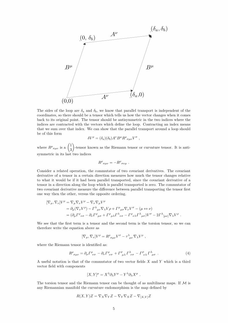
(0, δb)Aν

(δa, δb)

Bµ

(δa,0)Aν(0,0)

Bµ

The sides of the loop are δa and δb, we know that parallel transport is independent of thecoordinates, so there should be a tensor which tells us how the vector changes when it comesback to its original point. The tensor should be antisymmetric in the two indices where theindices are contracted with the vectors which define the loop. Contracting an index meansthat we sum over that index. We can show that the parallel transport around a loop shouldbe of this form

δV ρ = (δa)(δb)AνBµRρσµνV σ ,

where Rρσµν is a(

13

)-tensor known as the Riemann tensor or curvature tensor. It is anti-

symmetric in its last two indices

Rρσµν = −Rρσνµ .

Consider a related operation, the commutator of two covariant derivatives. The covariantderivative of a tensor in a certain direction measures how much the tensor changes relativeto what it would be if it had been parallel transported, since the covariant derivative of atensor in a direction along the loop which is parallel transported is zero. The commutator oftwo covariant derivative measure the difference between parallel transporting the tensor firstone way then the other, versus the opposite ordering.

[∇µ,∇ν ]V ρ = ∇µ∇νV ρ −∇ν∇µV ρ

= ∂µ(∇νV ρ)− Γλµν∇λV ρ+ Γ ρµσ∇νV σ − (µ↔ ν)= (∂µΓ ρνσ − ∂νΓ ρµσ + Γ ρµλΓ

λνσ − Γ ρνλΓλµσ)V σ − 2Γλ[µν]∇λV ρ .

We see that the first term is a tensor and the second term is the torsion tensor, so we cantherefore write the equation above as

[∇µ,∇ν ]V ρ = RρσµνVσ − τλµν∇λV ρ ,

where the Riemann tensor is identified as:

Rρσµν = ∂µΓρνσ − ∂νΓ ρνσ + Γ ρµλ Γ

λνσ − Γ ρνλ Γλµσ . (4)

A useful notation is that of the commutator of two vector fields X and Y which is a thirdvector field with components

[X,Y ]µ = Xλ∂λYµ − Y λ∂λXµ .

The torsion tensor and the Riemann tensor can be thought of as multilinear maps. If M isany Riemannian manifold the curvature endomorphism is the map defined by

R(X,Y )Z = ∇X∇Y Z −∇Y∇XZ −∇[X,Y ]Z

5

the notation ∇X refers to the covariant derivative along the vector field X, in components∇X = Xµ∇µ. The two vectors X and Y correspond to the two antisymmetric indices in thecomponent form of the Riemann tensor.

The curvature endomorphism is a(

13

)-tensor field.

Proof.

R(X, fY )Z = ∇X∇fY Z −∇fY∇XZ −∇[X,fY ]Z

= ∇X(f∇Y Z)− f∇Y∇XZ −∇f [X,Y ]+(Xf)Y Z

= (Xf)∇Y Z + f∇X∇Y Z − f∇Y∇XZ − f∇[X,Y ]Z − (Xf)∇Y Z= fR(X,Y )Z .

The same proof shows that R is linear over C∞(M) in X, because R(X,Y )Z = −R(Y,X)Zfrom the definition.

Here we used the Tensor characterization lemma which can be found in [5].Remark 2: The other case to be checked is the linearity over C∞(M) in Z, by following thesame procedure as above we see that this is indeed true.

If the components of the metric are constant in some coordinate system the Riemann tensorwill vanish, we can always construct a coordinate system in which the metric componentsare constant. It is necessary for the Riemann tensor to vanish for us to find components ofgµν that are constant everywhere. We choose Riemann normal coordinates at some pointp to be gµν = ηµν . Where ηµν is a matrix with either +1 or -1 for each diagonal elementand zero everywhere else. This is called locally inertial frame, i.e freely falling objects in agravitational field will not be able to detect the existence of a gravitational field.

Consider the components of this tensor in Riemann normal coordinates established at pointp. The Christoffel symbols will vanish but their derivatives will not so we have

Rρσµν = gρλ(∂µΓλνσ − ∂νΓλµσ)

= 12(∂µ∂σgρν − ∂µ∂ρgνσ − ∂ν∂σgρµ + ∂ν∂ρgµσ) .

From this we can infer three properties

• Rρσµν is antisymmetric in its first two indicesRρσµν = −Rσρµν .

• It is invariant under interchange of the first pair of indices with the secondRρσµν = Rµνρσ .

• The sum of cyclic permutations of the last three indices vanish:Rρσµν +Rρµνσ +Rρνσµ = 0 .

Riemann tensor obeys a differential identity which we will show in the following. Consider acovariant derivative of the Riemann tensor, evaluated in Riemann normal coordinates

∇λRρσµν = 12∂λ(∂µ∂σgρν − ∂µ∂ρgνσ − ∂ν∂σgρµ + ∂ν∂ρgµσ)

then considering the sum of cyclic permutations of the first three indices:

∇λRρσµν +∇ρRσλµν +∇σRλρµν = 12(∂λ∂µ∂σgρν − ∂λ∂µ∂ρgνσ − ∂λ∂ν∂σgρµ + ∂λ∂ν∂ρgµσ

+ ∂ρ∂µ∂λgσν − ∂ρ∂µ∂σgνλ − ∂ρ∂ν∂λgσµ + ∂ρ∂ν∂σgµλ

+ ∂σ∂µ∂ρgλν − ∂σ∂µ∂λgνρ − ∂σ∂ν∂ρgλµ + ∂σ∂ν∂λgµρ)= 0 .

6

This is a equation between tensors it is true in any coordinate system. Using theantisymmetry property Rρσµν = −Rσρµν allows us to write

∇[λRρσ]µν = 0 ,

this is known as the Bianchi identity. It can also be interpret as Jacobi identity[[∇µ,∇ν ],∇λ] = 0.

3.4 Ricci tensor and Ricci scalarSince 4-tensors are so complicated to calculate it is often useful to construct simpler tensorsthat summarize some of the information contained in the curvature. Consider contractionsof the Riemann tensor, even without the metric. We can form a contraction known as theRicci Tensor which is a covariant 2-tensor field as the trace of the Riemann tensor on itsfirst and last indices.

Rνγ = δµλRµνµγ = gµσg

σλRµνλγ . (5)

The Ricci tensor associated with the Christoffel connection is symmetric

Rµν = Rνµ ,

as a consequence of the various symmetries of the Riemann tensor. Using the metric gµν wecan take one further contraction and form Ricci scalar

R = Rµµ = gµνRµν .

Taking the contraction on the Bianchi identity twice we get

∇µRρµ = 12∇ρR .

If we define the Einsten tensor as

Gµν = Rµν −12Rgµν .

We see that the twice-contracted Bianchi identity implies

∇µGµν = 0 .

where Gµν is covariantly conserved of the stress-energy tensor.

Proof.

∇µGµν = ∇µ(Rµν −12Rgµν)

= ∇µRλµλν −12∇νR

= ∇µRλµλν −12∇νR

µλµλ

= ∇µRλµλν −12(−∇λRµλµλ −∇µR

µλµλ)

= ∇µRλµλν −12(∇λRλµλµ +∇µRλµλµ) = 0 .

(6)

The Einstein tensor is symmetric due to the symmetry of the Ricci tensor and the metric.

4 General Relativity“Matter tells space how to curve and space tells matter how to move”

-John Archibald Wheeler

7

This quote is a summary of General Relativity, how the gravitational field influences thebehavior of matter and how matter determines the gravitational field. In Newtoniangravity, these two aspects consist of the expression for the acceleration of a body ingravitational potential Φ. Gravitational fields are also conservative

a = −∇Φ .

By using Gauss Law we can express the field in terms of the volume of a sphere with amatter density and Newton’s gravitational constant we obtain

∇2Φ = 4πGρ .

General Relativity, which generalizes special relativity and Newton’s law of universalgravitation, describes the gravity as a geometric property of spacetime.

4.1 Einstein’s field equationsIn this section we will use a more modern approach to finding EFE’s, by taking the actionof a Lagrange density L and find the equation of motions. This was done by David Hilbertand this approach is known as the Einstein-Hilbert action. We can express the Lagrangedensity as

S =∫d4xL

where L = √−gR. Taking the variation of this action with respect to gµν , we obtain

δS =∫d4x

(√−ggµνδRµν +√−gRµνδgµν +Rδ

√−g). (7)

Let us first consider the first term in equation (7) which we will denote as δS1. By takingthe variation on the Riemann tensor we get the following equation

δRρσµν = ∂µδΓρνσ − ∂νδΓ ρµσ + δΓ ρµλ Γ

λνσ + Γ ρµλ δΓ

λνσ − δΓ ρνλ Γλµσ − Γ

ρνλ δΓ

λµσ . (8)

Where we used that any arbitrary variation can be written as Γ ρµν → Γ ρµν + δΓρµν andtherefore the variation is two different connections which in itself is a tensor. We can thencalculate the covariant derivative

∇λ(δΓ ρνµ ) = ∂λ(δΓ ρνµ ) + Γ ρσλ δΓσνµ − Γσνλ δΓ ρσµ − Γσµλ δΓ ρνσ . (9)

Now we look at the first term in the action and we see that we have to take the variation ofthe Ricci tensor.

δRµν = ∂λδΓρνµ − ∂νδΓ ρλµ + δΓ ρλσ Γ

σµν + Γ ρλσ δΓ

σµν

− δΓ ρσν Γσλµ − Γ ρσν δΓσλµ= ∂λδΓ

ρνµ − ∂νδΓ ρλµ + δΓ ρλσ Γ

σµν + Γ ρλσ δΓ

σµν

− δΓ ρσν Γσλµ − Γ ρσν δΓσλµ + Γσνλ δΓρσµ − Γσνλ δΓ ρσµ

=(∂λδΓ

ρνµ + Γσµν δΓ

ρλσ − Γσλµ δΓ ρσν − Γσνλ δΓ ρσµ

)−(∂νδΓ

ρλµ − Γ

ρλσ δΓ

σµν + Γ ρσν δΓ

σλµ − Γσνλ δΓ ρσµ

)= ∇λ(δΓ ρµν )−∇ν(δΓ ρµλ ) .

(10)

using this result we can rewrite δS1 in the following way

δS1 =∫d4x√−ggµν

[∇λ(δΓ ρµν )−∇ν(δΓ ρµλ )

]=∫d4x√−g

[∇λ(gµνδΓ ρµν )− δΓ ρµν∇λgµν −∇ν(gµνδΓ ρµλ ) + δΓ ρµλ∇νgµν

].

(11)

Going back to when we derived the Christoffel symbols, we used metric compatibility as acondition, i.e the covariant derivative is said to be compatible with the metric if thefollowing condition is satisfied

∇ρgµν = 0 .

8

Using this condition we then obtain the following action

δS1 =∫d4x√−g∇σ

[gµνδΓσµν − gµσδΓλλµ

]. (12)

Now we have to use Stokes theorem which relates the divergence of the vector field to itsvalue on the boundary. The vector field is the manifold M and the boundary is thehypersurface of the boundary Σ, then Stokes theorem is defined as∫

Md4x√|g|∇µV µ =

∫Σd3y√|γ|nµV µ . (13)

Now we use Stokes theorem on the action we obtain∫Md4x√|g|∇σ

[gµνδΓσµν − gµσδΓλλµ

]=∫

Σd3x√|h|nσ

[gµνδΓ ρµν − gµσδΓλλµ

], (14)

where nσ is the normal unit vector on the hypersurface which can be normalized tonσn

σ = −1. The tensor hµν is the induced metric on the hypersurface defined ashµν = gµν + nσn

σ. We integrate with respect to the volume element of the covariantdivergence of a vector. The boundary contribution at infinity can be set to zero, andtherefore the variation vanishes at infinity6.∫

Σd3x√|h|nσ

[gµνδΓ ρµν − gµσδΓλλµ

]= 0 .

So this term does not contribute to the action overall since it is zero.

Consider the third term now. We use the fact that for any square matrix M with nonvanishing determinant the following identity holds:

ln(detM) = Tr(lnM) .

The variation is then1

detM δ(detM) = Tr(M−1δM) .

Let us expand the determinant and obtain

g = gµνMµν

and then perform partial differentiation on both sides with respect to the metric

∂g

∂gµν= Mµν .

Consider the variation of the determinant g

δg = ∂g

∂gµνδgµν

= Mµνδgµν

= ggµνδgµν .

We can plug in the equation above and obtain

δ√−g = − 1

2√−g

= −12g√ggµνδg

µν .(15)

Rewriting the metric gives usδgµν = −gµβgνγδgβγ (16)

6Here we neglect the boundary term on the manifold M if we were to include the boundary term ∂Mthen we would have to take the variation on the action SEH + SGHY . Hence by only calculating SEH ourmanifold M is closed, for further details we refer to [7]

9

using this relation now and plugging it back into equation (15)

δ√−g = −1

2√−gggµνgµβgνγδgβγ

= −12δ

νβgµβδg

βγ

= −12√−ggβγδgβγ

= −12√−ggµνδgµν .

If we now take all the variations into consideration we can rewrite our Einstein-Hilbertaction (7) in the following way

δS =∫d4x√−g

[Rµν −

12Rgµν

]δgµν . (17)

The functional derivative of the action satisfies

δS =∫ ∑

i

(δS

δΦi δΦi

)dnx , (18)

where Φi is a complete set of fields being varied. So the stationary points are those wherethe boundary of the action terms are equal to zero, so we recover Einstein’s equation invacuum.

Rµν −12Rgµν = 0 . (19)

We would also want to obtain a non-vacuum field equation. We consider the action of theform

SEH = 18πGS + SM

where SM is the action for matter. Following the same procedure as above leads to

18πG

(Rµν −

12Rgµν

)+ 1√−g

δSMδgµν

= 0 (20)

and we recover Einstein’s equation if we set the stress-energy tensor to be

Tµν = − 1√−gδSMδgµν

.

We then recover the complete EFE’s

Rµν −12Rgµν = 8πGTµν , (21)

notice that the right hand side is from the Newtonian gravity where the density matter isexpressed in the Energy-momentum tensor. EFE’s can be thought of as a second orderdifferential equation for the metric tensor field gµν . The EFE’s are very complicated tosolve due to being a non-linear differential equations. It involves finding the Christoffelsymbols which we then need to find the Riemann tensor and then taking the contraction ofthe Riemann tensor yields us the Ricci tensor.

10

5 Black holesIn this section we will go through three black hole solutions to the EFE’s, the Schwarzschildsolution, the Reissner-Nordstrom solution and the Kerr-Newman solution. TheSchwarzschild solution is a static massive black hole. If we further add a charge we obtainthe Reissner-Nordstrom solution and if we add an angular momentum we obtain theKerr-Newman solution. These solutions present a black hole interpretation.

5.1 Schwarzschild solutionIn this section we will go through the derivation of the Schwarzschild solution as anexample just to see how to proceed in calculating EFE’s. This solution to the EFE’sdescribes the gravitational field outside a spherical mass where the electric charge of themass, angular momentum of the mass and the cosmological constant are all zero.

Figure 1: Schwarzschild geometry R× S2

Birkhoff’s TheoremAny spherically symmetric solution of the vacuum field equations must be static andasymptotically flat (curvature vanishes at large distances from some region, in other wordsthe larger the distance the closer the geometry becomes to that of Minkowski spacetime).This means that the exterior solution must be given by the Schwarzschild metric.

By using Birkhoff’s theorem, we can write our metric in the given form

ds2 = −e2α(t,r)dt2 + e2β(t,r)dr2 + r2dφ2 + r2 sin2 θdθ2 , (22)

where e2α(t,r) and e2β(t,r) are two positive functions which we need to evaluate in order toobtain the true solution. The Christoffel symbols can be obtained from equation (3) Themetric can be written in the matrix form, where all cross terms are zero

gµν =

−e2α(t,r)

e2β(t,r)

r2

r2 sin2 θ

The inverse metric components are then

gtt = −e−2α(t,r) , grr = e−2β(t,r) , gφφ = 1r2 , gθθ = 1

r2 sin2 θ

11

Γ ttt = 12g

tt (∂tgtt + ∂tgtt − ∂tgtt)

= −12e−2α(t,r)

(−2αte2α(t,r)

)= ∂tα ,

Γ ttr = 12g

tt (∂tgrt + ∂rgtt − ∂tgtr)

= −12e−2α(t,r)

(−2αre2α(t,r)

)= ∂rα ,

Γ trr = 12g

tt (∂rgrt + ∂rgtr − ∂tgrr)

= −12e−2α(t,r)

(−2βte2β(t,r)

)= e2(β−α)∂tβ ,

Γ rtt = 12g

rr (∂tgtr + ∂tgrt − ∂rgtt)

= 12e−2β(t,r)

(−2αre2α(t,r)

)= e2(α−β)∂rα ,

Γ rtr = 12g

rr (∂tgrr + ∂rgrt − ∂rgtr)

= 12e−2β(t,r)

(2αte2β(t,r)

)= ∂tβ ,

Γ rrr = 12g

rr (∂rgrr + ∂rgrr − ∂rgrr)

= 12e−2β(t,r)

(2αre2β(t,r)

)= ∂rβ ,

Γφrφ = 12g

φφ (∂rgφφ + ∂φgrr − ∂φgr0φ)

= 12

1r2(∂1r

2)= 1r,

Γ rφφ = 12g

rr (∂φgφr + ∂φgrφ − ∂rgφφ)

= 12e−2β(t,r) (−∂1r

2)= −re−2β(t,r) ,

Γ θrθ = 12g

θθ (∂rgθθ + ∂θgθr − ∂θgrθ)

= 12

1r2 sin θ

(∂rr

2 sin2 θ)

= 1r,

Γ rθθ = 12g

rr (∂θgθr + ∂θgrθ − ∂rgθθ)

= 12e−2β(t,r) (−∂1r

2 sin2 θ)

= −re−2β(t,r) sin2 θ ,

Γφθθ = 12g

φφ (∂θgθφ + ∂θgφθ − ∂φgθθ)

= 12

1r2(∂rr

2 sin2 θ)

= − sin θ cos θ ,

Γ θφθ = 12g

θθ (∂φgθθ + ∂θgθφ − ∂θgφθ)

= 12

1r2 sin2 θ

(∂rr

2 sin2 θ)

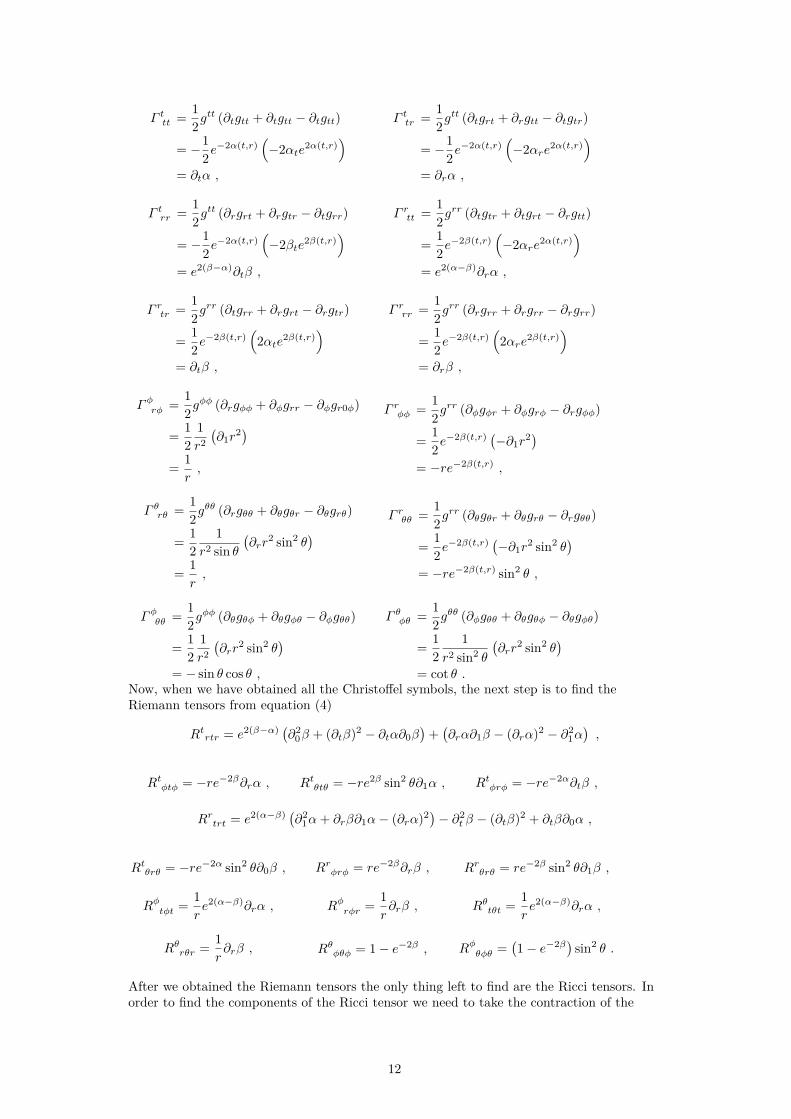
= cot θ .Now, when we have obtained all the Christoffel symbols, the next step is to find theRiemann tensors from equation (4)

Rtrtr = e2(β−α) (∂20β + (∂tβ)2 − ∂tα∂0β

)+(∂rα∂1β − (∂rα)2 − ∂2

1α),

Rtφtφ = −re−2β∂rα , Rtθtθ = −re2β sin2 θ∂1α , Rtφrφ = −re−2α∂tβ ,

Rrtrt = e2(α−β) (∂21α+ ∂rβ∂1α− (∂rα)2)− ∂2

t β − (∂tβ)2 + ∂tβ∂0α ,

Rtθrθ = −re−2α sin2 θ∂0β , Rrφrφ = re−2β∂rβ , Rrθrθ = re−2β sin2 θ∂1β ,

Rφtφt = 1re2(α−β)∂rα , Rφrφr = 1

r∂rβ , Rθtθt = 1

re2(α−β)∂rα ,

Rθrθr = 1r∂rβ , Rθφθφ = 1− e−2β , Rφθφθ =

(1− e−2β) sin2 θ .

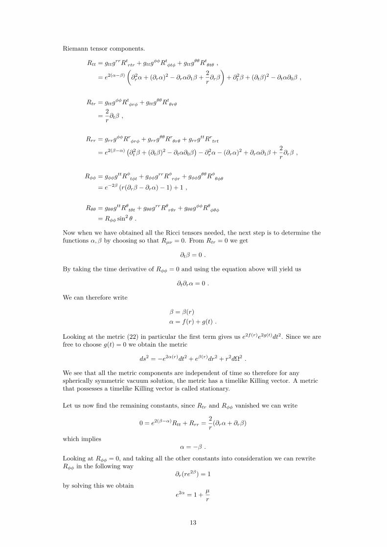
After we obtained the Riemann tensors the only thing left to find are the Ricci tensors. Inorder to find the components of the Ricci tensor we need to take the contraction of the

12

Riemann tensor components.

Rtt = gttgrrRtrtr + gttg

φφRtφtφ + gttgθθRtθtθ ,

= e2(α−β)(∂2rα+ (∂rα)2 − ∂rα∂1β + 2

r∂rβ

)+ ∂2

t β + (∂tβ)2 − ∂tα∂0β ,

Rtr = gttgφφRtφrφ + gttg

θθRtθrθ

= 2r∂tβ ,

Rrr = grrgφφRrφrφ + grrg

θθRrθrθ + grrgttRrtrt

= e2(β−α) (∂2t β + (∂tβ)2 − ∂tα∂0β

)− ∂2

rα− (∂rα)2 + ∂rα∂1β + 2r∂rβ ,

Rφφ = gφφgttRφtφt + gφφg

rrRφrφr + gφφgθθRφθφθ

= e−2β (r(∂rβ − ∂rα)− 1) + 1 ,

Rθθ = gθθgttRθtθt + gθθg

rrRθrθr + gθθgφφRθφθφ

= Rφφ sin2 θ .

Now when we have obtained all the Ricci tensors needed, the next step is to determine thefunctions α, β by choosing so that Rµν = 0. From Rtr = 0 we get

∂tβ = 0 .

By taking the time derivative of Rφφ = 0 and using the equation above will yield us

∂t∂rα = 0 .

We can therefore write

β = β(r)α = f(r) + g(t) .

Looking at the metric (22) in particular the first term gives us e2f(r)e2g(t)dt2. Since we arefree to choose g(t) = 0 we obtain the metric

ds2 = −e2α(r)dt2 + eβ(r)dr2 + r2dΩ2 .

We see that all the metric components are independent of time so therefore for anyspherically symmetric vacuum solution, the metric has a timelike Killing vector. A metricthat possesses a timelike Killing vector is called stationary.

Let us now find the remaining constants, since Rtr and Rφφ vanished we can write

0 = e2(β−α)Rtt +Rrr = 2r

(∂rα+ ∂rβ)

which impliesα = −β .

Looking at Rφφ = 0, and taking all the other constants into consideration we can rewriteRφφ in the following way

∂r(re2β) = 1

by solving this we obtaine2α = 1 + µ

r

13

the metric is then defined as

ds2 = −(

1 + µ

r

)dt2 +

(1 + µ

r

)−1dr2 + r2dΩ2 .

Now what is left is to determine the constant µ by using the weak field limit. We then seethat

gtt = −(1 + 2Φ)grr = (1− 2Φ) ,

with the potential Φ = −GM/r which is the Newtonian potential. Therefore the metricagrees with the limit when r →∞, if we set µ = −2GM .

The Schwarzschild metric then becomes

ds2 = −(

1− 2GMr

)dt2 +

(1− 2GM

r

)−1dr2 + r2dΩ2 .

This metric has two singularities: the first one is when r = 0 and the other one is whenr = rs where rs = 2M is the Schwarzschild radius. The Schwarzschild radius for the earthwould be approximately 8.9 millimeters meanwhile the sun’s radius would be 3 km.

Bending of starlight

In this section we will bring up a experimental verification of General Relativity. Theexperiment was done in 1919 by Sir Arthur Eddington though not very successful. Hetravelled to the west coast of Africa to observe the solar eclipse and measure the stars nearthe sun. His findings showed that the location of the star near the sun is not the stars trueposition and is instead a imaginary position. Let us demonstrate with a picture

We see that light bends so the true position of the star is in fact behind the sun and not atthe position we see the star at. So the spacetime does indeed change the direction of thelight and therefore we have a verification of Einstein’s theory of General Relativity. Let usdo a small calculation using the Schwarzschild metric with M being the mass of the Sun.We choose our angle to be θ = π/2 therefore we have sin θ = 1 and dθ = 0, we can nowwrite the metric in the following way

ds2 = −f(r)dt2 + dr2

f(r) + r2dφ2, f(r) = 1− 2MG

r(23)

Setting ds2 = 0 we can rewrite the metric as

dφ2 = 1r2

(f(r)dt2 − dr2

f(r)

). (24)

Choose φ as a affine parameter i.e we want to parameterize the geodesics curve by anarbitrary parameter. We choose ξ = ∂t which is a Killing vector and we obtain

ξµuµ = −C .

This is the integral of motion. We set

uµ = dlxµ

dφ

14

and obtain that ξt = 1 and ut = t′. Now our integral of motion becomes

C = −gttξtut = f(r)r2 t′ ⇒ 1 = r2

f(r)C2 − r′2

r2f(r) (25)

which after simplification gives us

r′2 = r4C2 − r2f(r) .

At maximum, when r = R, we get that r′ = 0. We therefore obtain that the constant canbe written as

C2 = f(r)R2 .

Plugging this into equation (24) gives us the following integral

2∫ ∞R

Rdr

r√r2f(r)−R2f(r)

=∫ π+∆φ

0dφ .

Evaluating the right side integral and substituting f(r) into the integral gives us

π + ∆φ = 2∫ ∞R

Rdr√r(r −R)((r2 −Rr)f(R)− 2MGR)

.

Making an approximation that RM under weak gravity we obtain

π + ∆φ = 2∫ ∞

1

dz

z√z2 − 1

+ 2M∫ ∞

1

z2 + z + 1z2(z + 1)

√z2 − 1

,

where ∆φ ≈ 4MR 1. So taking the Suns mass and the earth’s radius we obtain the angle

∆φ ≈ 8.5 ∗ 10−6 radiants. This calculation tells us that the spacetime curves the light,despite the angle being very small. But this is only due to the Sun’s mass not being largeenough for a significant result.

5.2 Reissner-Nordstrom SolutionThe Reissner-Nordstrom solution is also a static black hole but the difference between thissolution and the Schwarzschild solution is that this metric also has a charge. We obtain thecharge by solving the Einstein-Maxwell equations where we have a electromagneticstress-energy tensor and set the cosmological constant to zero. The metric is given in thefollowing form

ds2 = −(

1− rsr

+r2Q

r2

)dt2 +

(1− rs

r+r2Q

r2

)−1

dr2 + r2dΩ2 . (26)

If we let r2Q → 0 we obtain the Schwarzschild solution. This type of black hole has two

horizons, the event horizon and an internal Cauchy Horizon7

5.3 Kerr-Newman solutionThe Kerr-Newman metric is the solution to Einstein-Maxwell equations, where we nowhave a charged, rotating mass. We still assume that the cosmological constant is zero. Themetric is given in the following form

ds2 =−(

1− 2Mr −Q2

ρ2

)dt2 − 2a sin2 θ

(2Mr −Q2)ρ2 dtdφ+ ρ2

∆ dr2 + ρ2dθ2

+ sin2 θ

(r2 + a2 + a2 sin2 θ

2Mr −Q2

ρ2

)dφ2 .

(27)

7A Cauchy horizon is light-like domain that satisfies certain conditions which are given on a hypersurfacein the domian. For detailed discussion on this type of horizon we refer to [8]

15

the following definitions have been used

∆ = r2 − 2Mr + a2 +Q2

ρ2 = r2 + a2 cos2 θ

J = Ma .

If we were to set the angular momentum to zero we would obtain the Reissner-Nordstrommetric again, and setting the charge to zero we would end up with the Schwarzschild metric.The Kerr-Newman solution is a special case of more general exact solutions of theEinstein-Maxwell equations. The event horizons are the singularities defined as

r± = M ±√M2 − a2 −Q2 , (28)

where the positive singularity describes the outer event horizon and the negative singularitydescribes the inner horizon. This solution gives us a rotating black hole with an interestingattribute and that is that outside the event horizon we have a different horizon known asthe ergosphere8.

5.4 Black hole thermodynamicsIn this section we will go through the thermodynamics of black holes. We know that theblack holes need to have entropy in order not to violate the second law of thermodynamics.This section will cover the four laws of thermodynamics for black holes in order tounderstand how surface gravity relates to the temperature and the area of the event horizonwith the entropy. We will base this section on [10] and [11].

Zeroth Law

If the stress-energy tensor obeys the dominant energy condition then the surface gravity κgis constant on the future event horizon.

Definition 5. Tµν satisfies the dominant energy condition if for all future-directed timelikevector fields v, the vector field

j(v) ≡ −vµTµν , (29)is future-directed non-spacelike, or zero.

For simplicity we will not prove this and instead refer to [10] for a careful proof. Thesurface gravity is related to the temperature of the black hole, i.e the Hawking temperature

TH = κ

2π . (30)

First Law

Consider a stationary black hole of mass M , charge Q and angular momentum J withfuture event horizon of surface gravity κg. The electric surface potential ΦH and angularmomentum ΩH is perturbed such that when a black hole switches from one stationary toanother when taking the infinitesimal variation on the mass, charge and the angularmomentum, we then obtain

dM = κg8πdA+ ΩHdJ + ΦHdQ . (31)

Depending on the type of black hole the equation will be different, for example if we had aSchwarzschild black hole we would only have the first term, since this type of black hole hasno charge or no angular momentum. The first law with the second law together relates thearea of the event horizon with the entropy of the black hole. This is known as theBeckenstein-Hawking entropy defined as

SBH = A

4 . (32)

When we consider quantum mechanical effects the black holes then emit thermal radiationknow as Hawking radiation with the temperature defined in equation (33).

8For more detailed description on how to obtain the ergosphere, we refer to [6]

16

Second Law

If the stress-energy tensor satisfy the weak energy condition.

Definition 6. Weak energy condition

vµvµTµν ≥ 0 ∀non-spacelike v , (33)

then the area of the future event horizon of an asymptotically flat spacetime is anon-decreasing function of time.

dA

dt≥ 0 . (34)

This law can be violated when we take quantum effect into account, this was discovered byHawking. When black holes radiate away energy, the area and the mass of the black holewill decrease over time. Assume that the entropy is

S = SBH + Sext , (35)

where Sext is the entropy of matter in exterior spacetime. This suggest the generalized 2ndlaw of thermodynamics where equation (34) is always a non-decreasing function of time.This was suggested by Jacob Beckenstein, the meaning of this generalized 2nd law is that ifyou were to throw in mass into the black hole the exterior spacetime could decrease inentropy and this would violate the second law of thermodynamics unless the black hole hasan assigned entropy.

Third Law

It is not possible to form a black hole with vanishing surface gravity. κg = 0 is not possibleto achieve. Think of this as a thermodynamic system where T = 0 cannot be reached, sincewe know that the surface gravity is related to the temperature which implies the statementabove.

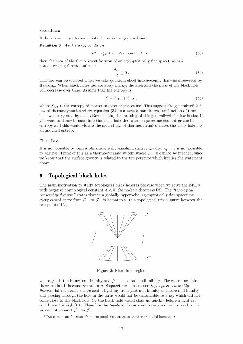
6 Topological black holesThe main motivation to study topological black holes is because when we solve the EFE’swith negative cosmological constant Λ < 0, the no-hair theorems fail. The “topologicalcensorship theorem” states that in a globally hyperbolic, asymptotically flat spacetimeevery casual curve from J− to J + is homotopic9 to a topological trivial curve between thetwo points [12],

J −

J +

Figure 2: Black hole region

where J + is the future null infinity and J− is the past null infinity. The reason no-hairtheorems fail is because we are in AdS spacetime. The reason topological censorshiptheorem fails is because if we sent a light ray from past null infinity to future null infinityand passing through the hole in the torus would not be deformable to a ray which did notcome close to the black hole. So the black hole would close up quickly before a light raycould pass through [13]. Therefore the topological censorship theorem does not work sincewe cannot connect J− to J +.

9Two continuous functions from one topological space to another are called homotopic

17

6.1 Geometrical structuresConsider the metric

ds2 = −V dt2 + V −1dr2 + r2σijdxidxj , (36)

where σij is the metric of a two-manifold, we assume that the metric does not describeneither topologically nor geometrically sphere and V = f(r). This metric will yield us threedifferent geometrical structures: a torus, sphere and a hyperbolic surface. These threesolutions will have different singularities describing the event horizon. Now when we try tosolve EFE’s our cosmological constant is negative (Λ < 0) where Λ = −3`−2. The onlynon-vanishing components of the Ricci tensor are

Rtt = −V 2Rrr = 12V V

′′ + V V ′

r, Rij = Rij − (rV ′ + V )σij

where Rij refers to the two-manifold. From this we obtain the function V which is given as

V = K − k′

r+ r2

`2(37)

which makes the metric satisfy the EFE’s with negative cosmological constant, Rµν = Λgµν .The reason this two-manifold generates three different solutions is because for the metric tosatisfy EFE’s we need to have constant curvature. The curvature does not need to be asphere, so if K = −q2 < 0 the two-manifold S must be a surface with constant negativecurvature. If the surface is compact and orientable then it must be a Riemann surface ofgenus g > 1 for q2 > 0. If q = 0 then the surface is a torus, and q = ±i/R gives a sphere ofradius R [9]. We can define the metric for a uncharged, genus-g black hole

ds2 = −(−1− 2η

r+ r2

`2

)dt2 +

(−1− 2η

r+ r2

`2

)−1

dr2 + r2σijdxidxj . (38)

Where Rij = −σij describes a Riemann surface with genus g > 1. This metric will be thekey component to obtain the surface gravity and event horizon temperature for black holeswith genus g > 1.

We start with the simplest case where our two-manifold describes a topological sphere. TheChristoffel symbols are

Γ trt = 12g

tt(∂rgtt + ∂tgtr − ∂tgtt)

= V ′

2V ,

Γ rtt = 12g

rr(∂tgtr + ∂tgtr − ∂rgtt)

= 12V V

′ ,

Γ rrr = 12g

rr(∂rgrr + ∂tgrr − ∂tgrr)

= − V′

2V ,

Γ rφφ = 12g

rr(∂φgφr + ∂φgφr − ∂rgφφ)

= −rV ,

Γ rθθ = 12g

rr(∂θgθr + ∂θgθr − ∂rgθθ)

= −rV sin2 θ ,

Γφφr = 12g

φφ(∂φgrφ + ∂rgφφ − ∂φgφφ)

= 1r,

Γφθθ = 12g

φφ(∂θgθφ + ∂θgθφ − ∂φgθθ)= − cos θ sin θ ,

Γ θθr = 12g

θθ(∂θgrθ + ∂rgθθ − ∂θgθr)

= 1r,

Γ θθφ = 12g

θθ(∂θgφθ + ∂φgθθ − ∂tθgθθ)= cot θ .

18

These are the Christoffel symbols for topological sphere. Now when we have these we canwrite down the Riemann tensor components for this metric

Rtrrt = V ′′

2V , Rtφφt = 12rV

′ , Rtθθt = 12rV

′ sin2 θ ,

Rrtrt = 12V V

′′ , Rrφφr = rV ′

2 , Rrθθr = 12rV

′ sin2 θ ,

Rφtφt = V V ′

2r , Rφrφr = − V ′

2rV , Rφθθφ = (−1 + V ) sin2 θ ,

Rθtθt = V V ′

2r , Rθrθr = − V ′

2rV , Rθφθφ = 1− V .

These are the non-vanishing Riemann tensor components. We can now finally obtain theRicci tensor components

Rtt = −gttgrrRtrtr − gttgφφRtφtφ − gttgθθRtθtθ

= V

2

(V ′′ + 2V ′

r

),

Rrr = grrgttRrrtr − grrgφφRrφrφ − grrgθθRrθrθ

= −2V ′ + rV ′′

2rV ,

Rφφ = gφφgttRφtφt + gφφg

rrRφrφr − gφφgθθRφθφθ

= 1− V − rV ′ ,

Rθθ = gθθgrrRθrθr + gθθg

φφRθφθφ + gθθgttRθtθt

= − sin2 θ(−1 + V + rV ′) .

We can now solve Rµν = Λgµν to obtain the non-vanishing differential equations.

Gtt = V

2

(−−6`2

+ 2V ′r

+ V ′′),

Grr = −(−−6`2 + 2V ′

r + V ′′

2rV

),

Gφφ = 1 + 3r2

`2− V − rV ′ ,

Gθθ = sin2 θ

(1 + 3r2

`2− V − rV ′

).

Choosing Gφφ = 0 and solving this equation gives us that the function V (r)

V (r) = 1− 2ηr

+ r2

`2.

Then the metric is defined as

ds2 = −(

1 + k′

r+ r2

`2

)dt2 +

(1 + k′

r+ r2

`2

)−1

+ r2dΩ2 . (39)

This is the Schwarzschild solution with a negative cosmological constant if we set k′ = −2ηwhere η is the mass of the object10.

10It is often called the Schw-AdS metric

19

For the torus case we need to define some things first. Since a torus has genus g = 1 weintroduce a complex parameter τ11. This complex number specifies a class of conformallyequivalent tori i.e if there exist an angle preserving transformation such as a Mobiustransformation

f(z) = az + b

cz + d.

So in order for the two tori to be equivalent if and only if the complex parameters areconnected by a Mobius transformation with an integer coefficient. We can therefore rewritethe flat metric of the torus as

dσ2 = |τ |2dx2 + dy2 + 2 Re τdxdy .

Let us derive the torus case to see that we actually get the non-vanishing Ricci tensorsgiven above. We start by writing the metric in matrix form and its inverse.

ds2 =

−V 0 0 00 V −1 0 00 0 r|τ |2 r2 Re τ0 0 r2 Re τ r2

(40)

and the inverse matrix

ds2 =

V −1 0 0 0

0 V 0 00 0 1

r2τ22− τ1r2τ2

2

0 0 − τ1r2τ2

2

|τ |2r2τ2

2

(41)

where τ = τ1 + iτ2. We can now obtain the Christoffel symbols using the equation (3).

Γ trt = 12g

tt(∂rgtt + ∂tgtr − ∂tgtt)

= V ′

2V ,

Γ rtt = 12g

rr(∂tgtr + ∂tgrt − ∂rgtt)

= V V ′

2 ,

Γ rrr = 12g

rr(∂rgrr + ∂rgrr − ∂rgrr)

= V ′

2V ,

Γ rφφ = 12g

rr(∂φgφr + ∂φgφr − ∂rgφφ)

= −rV |τ |2 ,

Γ rθφ = 12g

rr(∂θgφr + ∂φgrθ − ∂rgθφ)

= −rV τ1 ,Γ rθθ = 1

2grr(∂θgθr + ∂θgθr − ∂rgθθ)

= −rV ,

Γφφr = 12g

φφ(∂φgrφ + ∂rgφφ − ∂φgφr)

= 1r,

Γ θθr = 12g

θθ(∂θgrθ + ∂rgθθ − ∂θgθr)

= 1r.

These are the non-vanishing Christoffel symbols, now we can obtain the Riemann tensors forthis metric by using the equation (4). The non-vanishing Riemann tensor components are

Rtφφt = V ′′

2V , Rtθθt = 12r|τ |

2V ′ , Rtφθt = 12rτ1V

′ ,

Rtθφt = 12rτ1V

′ , Rtθθt = 12rV

′ , Rrrtr = 12V V

′′ ,

Rrφφr = 12r|τ |

2V ′ , Rrφθr = 12rτ1V

′ , Rrθφr = 12rτ1V

′ ,

11this is known as the Teichmuller complex parameter

20

Rrθθr = 12rV

′ , Rθtθt = V V ′

2r , Rθφθφ = − V ′

2rV ,

Rφφθφ = τ1V , Rφθθφ = V , Rθtθt = V V ′

2r ,

Rθrθr = − V ′

2rV , Rθφθφ = −|τ |2V , Rθθθφ = −τ1V ,

the calculations for the Riemann tensors can be found in the appendix B. Now when wehave obtained the Riemann tensor, we can finally obtain the Ricci tensors, using theequation (5)

Rtt = −gttgrrRtrtr − gttgφφRtφtφ − gttgθθRtθtθ

= V

2

(V ′′ + 2V ′

r

),

Rrr = grrgttRrrtr − grrgφφRrφrφ − grrgθθRrθrθ

= −2V ′ + rV ′′

2rV ,

Rφφ = gφφgttRφtφt + gφφg

rrRφrφr − gφφgθθRφθφθ

= −|τ |2(rV ′ + V ) ,

Rθφ = −gθθgθφRθrφr − gθθgθφRθtφt − gθθgθφRθθφθ= τ1(rV ′ + V ) ,

Rθθ = gθθgrrRθrθr + gθθg

φφRθφθφ + gθθgttRθtθt

= −rV ′ − V .

These are the non-vanishing Ricci tensors, the only thing left to do now is to solve theEFE’s Rµν = Λgµν . The Einstein tensors are then given as

Gtt = V

2

(−−6`2

+ 2V ′r

+ V ′′),

Grr = −(−−6`2 + 2V ′

r + V ′′

2rV

),

Gφφ = |τ |2(−V + r

(3r`2− V ′

)),

Gφθ = 3r2τ1`2− τ1(V + rV ′) ,

Gθφ = 3r2τ1`2− τ1(V + rV ′) ,

Gθθ = −V + r

(3r`2− V ′

).

Choosing the simplest Einstein tensor and solving the differential equation Gµν = 012. Sofor example choosing Gθθ = 0 gives us that the function V (r) which in the torus case is

V (r) = −2ηr

+ r2

`2,

12The reason we choose the simplest is because it is the easiest one to calculate, the others are morecomplicated due to being 2nd order ODE.. Actually choosing any Gµν = 0 will give us the same functionV (r), this can be checked for any given Einstein tensor by using for example Mathematica.

21

where K = 0 because the constant curvature is zero if the surface is a torus. The metric isthen given as

ds2 = −(−2ηr

+ r2

`2

)dt2 +

(−2ηr

+ r2

`2

)−1

dr2 + r2(|τ |2dx2 + dy2 + 2 Re τdxdy) . (42)

We can define the area of these type of black holes with a genus g ≥ 1, by introducingGauss-Bonnet theorem.

Definition 7. Let S be an oriented compact two-manifold with a Riemannian manifold withboundary ∂S. Let C be the Gaussian curvature of S, and let kg be the geodesics curvatureof ∂S. Then ∫

S

KdA+∫∂S

kgds = 2πχg ,

where dA is the surface area and χg is the Euler characteristic number defined asχg = 2− 2g where g is the number of holes [5].

The Euler characteristic number is equal to two if the manifold S is a sphere, zero when itis a torus and 2− 2g if the manifold is a orientable surface of genus g. If a compactorientable surface has negative Gaussian curvature the Gauss-Bonnet theorem forces thegenus to be g > 1.

The area of manifold S is then defined as

A = −2πχg + | Im τ |δ(g, 1) = 4π(g − 1) + | Im τ |δ(g, 1) . (43)

This is the area of the black holes, this area is very important when discussing the entropyof the black holes as we saw from the formulation in section 4.4. Let us now discuss thesingularities in the two cases. When the curvature becomes infinite our interpretation of thesingularities are wrong. One could say that if the curvature invariant13 does not blow up wehave chosen a bad coordinate system14. In the case where r = 0 we see that the curvatureinvariant RµνρσRµνρσ = r−6 blows up when r = 0 so therefore this is a good singularity. Soin our case we should study the metric when r > 0. We now need to solve cubic equationgiven in the metric for the general case i.e r3 − `2r − 2η`2 = 0. Every cubic equation has atleast one solution therefore we can find information about the nature of the roots by usinga discriminant D = η2`4 − `6/27, since we only study positive sign of the roots we end upwith the following root

r+ = 21/3`2

3[2η`2 + 2(D)1/2]1/3 + [2η`2 + 2(D)1/2]1/321/3 . (44)

This is the only real root, where we chose D > 0 and η > 0. Since the root is positive thesingularity is spacelike and located inside the event horizon.

6.2 Surface gravity and TemperatureIn the section black hole thermodynamics where we said that the zeroth law of BHthermodynamics relates the surface gravity to the temperature of the surface. So thereforewe can formulate the temperature of these topological black holes by finding the surfacegravity and relating it to the Hawking temperature. The surface gravity for thesetopological black holes are defined as

κ =3r2

+ +K`2

2r+`2. (45)

Here C describes the curvature for the black holes, for example for the torus case K = 0,and for the case when g > 1 we have that K = −1. For the derivation of the surface gravity

13curvature invariant are scalar quantities14This method is quite simply since we found our answer by only taking the forth order Ricci scalar. In

general you have to consider all possible curvature invariants in order to say something about the singularitiesof the curvature and this is not a valid approach since it would take infinite long.

22

we refer the reader to appendix C. One of the approaches to finding the temperature is todo a Wick rotation to imaginary time t→ iτ on the metric. We saw that the only positiveroot was defined as (43) which was said to be a root that is located inside the eventhorizon, so therefore it would only make sense for us to investigate the temperature whenwe are at r = r+. We start with the metric (36)

ds2 = −f(r)dt2 + dr2

f(r) + r2dΩ22 .

We then define the constantρ2 = λf(r) .

Since we choose to be at the event horizon we set r = r+ and use the Wick rotation then weobtain the following metric

ds2 = ρ2

λdτ2 + 4

λ(f ′(r))2 dρ2 + r2

+dΩ22 . (46)

Now we need to identify the time coordinate with the periodicity 2π, we then see thatτ√λ∈ [0, 2π]. Relating this to the temperature we obtain

TBH = 12π√λ

= f ′(r+)4π . (47)

We can now find the constant λ to obtain the temperature for each topological black holeby just taking the derivative with respect to the radial component of f(r), we then see that

d

drf(r) = 2η

r2 + 2r`2

∣∣∣∣r=r+

=3r2

+ +K`2

r+`2.

Which is exactly the surface gravity we obtain by choosing the right curvature constant, wecan identify the temperature for the given structure. Hence the temperature for the g > 1case and g = 1 are

TBH =3r2

+ − `24πr+`2

, TBH = 3r+4π`2 . (48)

We see that in order to obtain the temperature we need to identify the time coordinatewith the right periodicity, which is 2π. Since we are treating the black holes with quantumeffects, the temperature has to be equal to the Hawking temperature in order for thequantum effects to be in equilibrium with the black hole.

• At any other temperature, the Euclidean metric of these topological black holes willhave a conical singularity, which means that there is no equilibrium

• Equilibrium at Hawking temperature is unstable since, if the black hole absorbsradiation its mass increases and its temperature decreases, i.e the black holes hasnegative specific heat. [10]

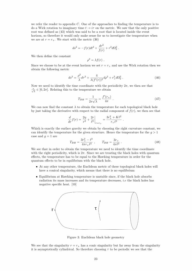
Figure 3: Euclidean black hole geometry

We see that the singularity r = r+ has a conic singularity but far away from the singularityit is asymptotically cylindrical. So therefore choosing τ to be periodic we see that the

23

Hawking temperature is T = κ2π where κ is the surface gravity which was what we obtained

in the derivation. The stability condition criteria is fulfilled when the black hole equilibriumis unstable by looking at the Hawking temperature of the black hole, i.e if the heat capacityof the black hole is positive then this condition is fulfilled.

To see that the heat capacity is positive we need to define what the mass of the black holeis, using the mass defined in [9] we get the following mass for the topological black holes

M = (η − η0)(g − 1) + η| Im τ |4π δ(g, 1) . (49)

Using the equation (44) and equation (48) we can formulate the mass as a function of thetemperature, this can be obtained by expressing r+ in terms of the temperature for g > 1and g = 1

r+ = 2π`2T3

(1 +

√3

4π2`2T 2

), r+ = 4π`2T

3 ,

so for g > 1 case we get the formula

M = (g − 1)4π3`4T 3

27

(1 +

√3

4π2`2T 2

)((2 + 3

4π2`2T 2 + 2√

1 + 34π2`2T 2 − `2

))− η0(g − 1) ,

(50)

and for the g = 1 case we get

M = | Im τ |8π2`4T 3

27 . (51)

Therefore using the heat capacity formula

Cv = ∂M

∂T, (52)

we see that by taking the derivative with respect to temperature of the mass functions wewould obtain a positive heat capacity. Since both mass functions are ∂M

∂T > 0, therefore thestability condition is fulfilled. If we would do the same procedure to the EuclideanSchwarzschild metric we would obtain that the heat capacity is negative and is an unstablethermodynamic system. For the calculation i refer you to the appendix D.

7 DiscussionWe first started with reviewing the solutions to the EFE’s for a static uncharged black holeknown as the Schwarzschild black hole, where Birkhoff’s theorem states that any sphericallysymmetric solution of the vacuum field equations must be static and asymptotically flat.The Schwarzschild solution has a spherical horizon in which the no-hair theorems apply aswell as topological censorship. Solutions to EFE’s have spherical horizon and obeythermodynamic laws like the asymptotically flat black holes.

We then solved EFE’s with a negative cosmological constant (Λ < 0) with a metriccontaining a two-manifold that didn’t have to be a topological sphere, but instead thesolution could admit a toroidal black hole with genus g ≥ 1. This is quite interesting sinceit would violate the topological censorship as well as the no-hair theorems. So the questionarises whether these topological black holes could obey thermodynamical laws like theasymptotically flat black holes. In order to show that these black holes obeythermodynamics we had to define the horizons of the metric and investigate the nature ofthe roots, in order to find a good singularity. The only real singularity was when r = r+which was located inside the event horizon. In section 6.2 we used the Euclidean approachto find the Hawking temperature of the event horizon for the given genus-g black hole. Inorder to obtain the Hawking temperature we had to identify the time coordinate with theright periodicity. Figure (3) described how the black holes are in equilibrium with quantumeffects at the singularity. Our singularity had conical geometry so therefore the topological

24

black hole is not in equilibrium with the system. Such an equilibrium at the Hawkingtemperature is said to be unstable if its mass increases while its temperature decreaseswhen the black hole absorbs radiation i.e the heat capacity is negative. We showed that theheat capacity for Schwarzschild black hole is indeed negative and therefore is unstable.Meanwhile the stability condition ∂M

∂T > 0 for the topological black holes is positive andthey are in fact stable black holes. Let us look more closely on the mass equations (50) and(51) where M is a function of T . We see that at very high temperatures (T →∞) therelation between mass and temperature is M ∼ T 3. Since the topological black holes arestable one can assume that the universe they live in is very hot. They could even existduring the inflationary era. This would mean that the black holes are colder than theenvironment, so if the black holes have relatively high temperature the mass of the blackholes will also be massive.

The conclusion is that we can have topological black holes that obey thermodynamical lawslike the asymptotically flat black holes with spherical horizon. The topological censorshipdoes not apply to topological black holes with genus-g horizon because they close up tooquickly in order to connect the past null infinity to the future null infinity. Nevertheless wecan have topological black holes that indeed obey thermodynamical laws.

Black holes are interesting objects with a collection of challenging problems such as theinformation loss paradox. In String theory one tries to combine General Relativity andQuantum field theory. Since the universe we live in is not classical but quantum mechanicalit would only make sense to combine General Relativity with Quantum field theory toexplain for example black holes and its entropy.

AcknowledgmentsI would like to thank my supervisor Giuseppe Dibitetto, for the valuable input and takingtime and effort to answer my questions. Without his input I might never have beenintroduced to these topics. I would also like to thank my family and friends for encouragingme to continue my studies. Susanne Mirbt for her guidance and helpful advice.

References[1] Birkhoff, G. D. Relativity and Modern Physics Cambridge, Massachusetts:

Harvard University Press (1923)

[2] S.Hawking and G.F Ellis The large scale structure of spacetime, CambridgeUniversity Press (1973)

[3] S.Hawking Black holes in General Relativity Commun, math. Phys. 25 (1972)

[4] Jurgen Just Riemannian geometry and geometric analysis Springer-Verlag(2002)

[5] John M. Lee Riemannian manifolds, An introduction to curvatureSpringer-Verlag (1997)

[6] Sean M.Carroll Lecture notes on General Relativity gr-qc/9712019 (1997)

[7] Gibbsons, G.W and S.W Hawking Action integrals and partition functions inquantum gravity Physical review D 15 (1977)

[8] S.Chandrasekhar The mathematical theory of black holes Oxford Classictexts in the Physical Sciences (1983)

[9] L.Vanzo Black holes with unusual topology arXiv:gr-qc/9705004v3 (1997)

[10] P.K Townsend Lecture notes on Black holes arXiv:gr-qc/9707012 (1997)

[11] Simon F.Ross Black hole thermodynamics arXiv:hep-th/0502195

25

[12] J.L. Friedmann, K.Schleich and D.M. Witt. Topological censorship theoremPhys.Rev.Lett 71, 1486 (1993)

[13] T.Jacobsen and S.Venkataramani Topology of event horizon and topologicalcensorship Class. Quantum Grav (1995)

26

AppendicesA Schwarzschild solution

Rtrtr = ∂tΓtrr − ∂rΓ ttr + Γ tλt Γ

λrr − Γ trλ Γλtr

= ∂tΓtrr − ∂rΓ ttr + Γ ttt Γ

trr + Γ ttr Γ

rrr − Γ trt Γ ttr − Γ trr Γ rtr

= e2(β−α) (∂20β + (∂tβ)2 − ∂tα∂0β

)+(∂rα∂1β − (∂rα)2 − ∂2

1α)

Rtφtφ = ∂tΓtφφ − ∂φΓ ttφ + Γ ttλ Γ

λφφ − Γ rrλ Γλtφ

= ∂tΓφφφ − ∂φΓ ttφ + Γ ttλ Γ

λφφ − Γ rrλ Γλtφ

= −re−2β∂rα

Rtθtθ = ∂tΓtθθ − ∂θΓ ttθ + Γ ttr Γ

rθθ − Γ tθλ Γλθθ

= ∂tΓtθθ − ∂θΓ ttθ + Γ ttr Γ

rθθ − Γ tθλ Γλθθ

= −re2β sin2 θ∂1α

Rtφrφ = ∂tΓtφφ − ∂φΓ trφ + Γ trλ Γ

λφφ − Γ trλ Γλrφ

= ∂rΓtφφ − ∂φΓ trφ + Γ trr Γ

rφφ − Γ trφ Γφrφ

= −re−2α∂tβ

Rrtrt = ∂rΓrtt − ∂tΓ rrt + Γ rrλ Γ

λtt − Γ rtλ Γλrt

= ∂rΓrtt − ∂tΓ rrt + Γ rrt Γ

ttt + Γ rrr Γ

rtt − Γ rtt Γ trt − Γ rtr Γ rrt

= e2(α−β) (∂21α+ ∂rβ∂1α− (∂rα)2)− ∂2

t β − (∂tβ)2 + ∂tβ∂0α

Rtθrθ = ∂rΓtθθ − ∂θΓ trθ + Γ trλ Γ

λθθ − Γ tθλ Γλrθ

= ∂rΓtθθ − ∂θΓ trθ + Γ trr Γ

rθθ + Γ trφ Γ

φθθ − Γ tθθ Γ θrθ

= −re−2α sin2 θ∂0β

Rrφrφ = ∂rΓrφφ − ∂rΓ rrφ + Γ rrλ Γ

λφφ − Γ rφλ Γλrφ

= ∂rΓrφφ − ∂φΓ rrφ + Γ rrr Γ

rφφ − Γ rφφ Γφrφ

= re−2β∂rβ

Rrθrθ = ∂rΓrθθ − ∂θΓ rrθ + Γ rrλ Γ

λθθ − Γ rθλ Γλrθ

= ∂rΓrθθ − ∂θΓ rrθ + Γ rrr Γ

rθθ + Γ rrφ Γ

φθθ − Γ rθθ Γ θrθ

= re−2β sin2 θ∂1β

Rφtφt = ∂φΓφtt − ∂tΓφφt + Γφφλ Γλtt − Γφtλ Γλφt

= 1re2(α−β)∂rα

Rφrφr = ∂φΓrtt − ∂rΓφφr + Γφφλ Γ

λrr − Γφrλ Γλφr

= 1r∂rβ

27

Rθtθt = ∂θΓθtt − ∂tΓθθt + Γ θθλ Γλtt − Γ θrλ Γλθt

= 1re2(α−β)∂rα

Rθrθr = ∂θΓθrr − ∂rΓθθr + Γ θθλ Γλrr − Γ θrλ Γλθr

= 1r∂rβ

Rθφθφ = ∂θΓθφφ − ∂φΓφφr + Γ θθλ Γλφφ − Γ θφλ Γλθφ

= 1− e−2β

Rφθφθ = ∂rΓφθθ − ∂θΓ

φφθ + Γφφλ Γ

λθθ − Γφθλ Γ

φφθ

= ∂φΓφθθ − ∂θΓ

φφθ + Γφφφ Γ

φθθ − Γ

φθθ Γ

θφθ

=(1− e−2β) sin2 θ

B Riemann tensors for torus case

Rtrrt = ∂rΓttr − ∂tΓ rφφ − Γ ttλ Γλrr + Γ trλ Γ

λtr

= −Γ ttr Γφφφ + Γ trt Γtrt

= V ′′

2V

Rtφφt = ∂φΓttφ − ∂tΓ rθθ − Γ ttλ Γλφφ + Γ tφλ Γ

λtφ

= −Γ ttr Γφθθ= 1

2r|τ |2V ′

Rtφθt = ∂θΓttφ − ∂tΓ tθφ − Γ ttλ Γλθφ + Γ tθλ Γ

λtφ

= −Γ ttr Γ rθφ= 1

2rτ1V′

Rtθφt = ∂φΓttθ − ∂tΓ tφθ − Γ ttλ Γλφθ + Γ tφλ Γ

λtθ

= −Γ ttr Γ rφθ= 1

2rτ1V′

Rtθθt = ∂θΓttθ − ∂tΓ tθθ − Γ ttλ Γ ttλ Γλθθ + Γ tθλ Γ

λtθ

= −Γ ttr Γ rθθ= 1

2rV′

28

Rφrφr = ∂rΓrtt − ∂tΓ rrt − Γ rtλ Γλrt

= ∂r(12V V

′)− Γ rtt Γ trt + Γφφφ Γrtt

= 12V V

′′

Rrφφr = ∂φΓrrφ − ∂rΓφθθ − Γ rrλ Γλφφ + Γφφλ Γ

λrφ

= ∂r(r|τ |2V )− Γφφφ Γφθθ + Γφθθ Γ

θφθ

= 12r|τ |

2V ′

Rrφθr = ∂θΓrrφ − ∂rΓ rθφ − Γ rrλ Γλθφ + Γ rθλ Γ

λrφ

= ∂r(rτ1)− Γφφφ Γ rθφ + Γ rθφ Γθφθ

= 12rτ1V

′

Rrθφr = ∂φΓrrθ − ∂rΓ rφθ − Γ rrλ Γλφθ + Γ rφλ Γ

λrθ

= ∂r(rτ1V )− Γφφφ Γ rφθ + Γ rφθ Γθrθ

= 12rτ1V

′

Rrθθr = ∂θΓrrθ − ∂rΓ rθθ − Γ rrλ Γλθθ + Γ rθλ Γ

λrθ

= ∂r(rV )− Γ rθθ Γ θrθ + Γφφφ Γrθθ

= 12rV

′

Rθrθr = ∂φΓφtt − ∂tΓφφt − Γ

φtλ Γ

λφt + Γφφλ Γ

λtt

= Γφφr Γrtt

= V V ′

2r

Rθφθφ = ∂φΓφrr − ∂rΓφφr − Γ

φrλ Γ

λφr + Γφφλ Γ

λrr

= −∂r(1r

)− Γ θφθ Γφφr + Γφφr Γφφφ

= − V ′

2rV

Rφφθφ = ∂θΓφφφ − ∂φΓ

φθφ − Γ

φφλ Γ

λθφ + Γφθλ Γ

λφφ

= −Γφφr Γ rθφ= τ1V

Rφθθφ = ∂θΓφθθ − ∂φΓ

φθθ − Γ

φφλ Γ

λθθ + Γφθλ Γ

λφθ

= −Γφφr Γ rθφ= V

29

Rθtθt = ∂θΓθtt − ∂tΓ θθt − Γ θtλ Γλθt + Γ θθλ Γ

λtt

= Γ θθr Γrtt

= V V ′

2r

Rθrθr = ∂θΓθrr − ∂rΓ θθr − Γ θrλ Γλθr + Γ θθλ Γ

λrr

= −∂r(1r

)− Γ θrθ Γ θθr + Γ θθr Γφφφ

= − V ′

2rV

Rθφθφ = ∂θΓθφφ − ∂φΓ θθφ − Γ θφλ Γλθφ + Γ θθλ Γ

λφφ

= Γ θθr Γφθθ

= −|τ |2V

Rθθθφ = ∂θΓθφθ − ∂φΓ θθθ − Γ θφλ Γλθθ + Γ θθλ Γ

λφθ

= Γ θθr Γrφθ

= −τ1V

C Surface gravityWe use the formula which can be found in [6], where the surface gravity is defined as

κ2 = −12(∇aχb)(∇aχb)

Where χa is the Killing field for the horizon. The Killing vector is our case can be written as

χa ∼ (K − 2ηr

+ r2

`2, 0, 0, 0)

if one were to be sure that this was true you could obtain the Christoffel symbols Γ trt andΓ rtt and see that χaχa = 0 when r = r+, where r+ is the positive root located inside theevent horizon. Calculating ∇rχt gives us that

∇rχt =3r2

+ +K`2

2r+`2= −∇tχr

Using the equation given above gives us

κ2 = −12(∇tχr∇tχr +∇rχt∇rχt)

= −12(−∇tχr∇tχr −∇rχt∇rχt)

= ∇tχr∇tχr =(3r2

+ +K`2

2r+`2

)2

therefore the surface gravity is

κ =3r2

+ +K`2

2r+`2

where C stands for the curvature, where K = 0 gives a torus and K = −1 gives us a g > 1object.

30

D Heat capacity for Schwarzschild metricUsing the first law of black hole thermodynamics we see that the mass is related to thesurface gravity

dM = κ

8πdA

Using the Euclidean Schwarzschild solution

ds2 = ρ2

16M2 dτ2 + dρ2 + 4M2dΩ2

where we used Wick rotation to obtain the imaginary time, and identifying the imaginarytime to be periodic, we can therefore obtain the Hawking temperature for this metric whichis

T = 18πM

Using the free energy F (T, V ) which we can relate the mass and the first law of black holethermodynamics to, we the obtain that the free energy can be written as

F = 116πT

Now using the heat capacity formula we obtain

C = ∂E

∂T= −T ∂

2F

∂T 2 = −8πM2

here we see that the heat capacity is negative therefore the Schwarzschild metric is anunstable thermodynamic system.

31