Chapter 4

Geodesics of the Kerrmetric

Here we will study the geodesic motion outside a Kerr black hole;therefore, we will only consider the region outside the outer horizon,

r ! r+ (4.1)

which is the relevant region for astrophysical considerations.Let us consider a geodesic with a!ne parameter ! and tangent

vector

uµ =dxµ

d!" xµ (4.2)

in Boyer-Linquist coordinates (we remind that, in our conventions,the overdot has the meaning of derivation with respect to the a!neparameter !). The tangent vector uµ is solution of the geodesicequation

uµu!;µ = 0 . (4.3)

The geodesic equation (4.3) is equivalent to the Euler-Lagrangeequations

d

d!

"L"x"

="L"x"

(4.4)

associated to the Lagrangian

L (xµ, xµ) =1

2gµ! x

µx! . (4.5)

One can define the conjugate momentum pµ to the coordinate xµ as

pµ " "L"xµ

= gµ! xµ . (4.6)

67

In terms of the conjugate momenta, the Euler-Lagrange equationscan be written as

d

d!pµ =

"L"xµ

. (4.7)

Notice that, if the metric does not depend on a given coordinate xµ,the corresponding conjugate momentum is a constant of motion.The existence of such a constant can also be seen in a simpler way.We know that, if the metric is independent by a coordinate, thereis a Killing vector #µ corresponding to this symmetry, and #µxµ

is a constant of geodesic motion; actually, this constant of motioncoincides with the one arising from Euler-Lagrange equations (as wewill see, for instance, in the case of t and $ for the Kerr metric).

Let us come back to the geodesic equation for Kerr spacetime.Equation (4.3) (or, equivalently, (4.4)) in Kerr spacetime is verycomplicate to solve directly. To study geodesic motion in a simpleway, we would need to find a way to express the geodesic uµ in termsof conserved quantities, as we have done in the case of Schwarzschildspacetime. For this, we need four algebraic relations involving uµ.

As we have seen in Section 3.2, Kerr spacetime has two Killingvectors: a timelike Killing vector kµ = (1, 0, 0, 0) and a spacelikekilling vector mµ = (0, 0, 0, 1). This corresponds to the fact that themetric (in Boyer-Lindquist coordinates) does not depend explicitlyby t and $: the spacetime is stationary and axially symmetric.

Therefore, in geodesic motion there are two conserved quantities:

E " #kµuµ = #gtµu

µ = #pt constant along geodesics

(4.8)

L " mµuµ = g#µu

µ = p# constant along geodesics .

(4.9)

As explained in Section 3.2, in the case of massive particle E is theenergy at infinity per mass unit while L is the angular momentumper mass unit; in the case of massless particles, E is the energy atinfinity and L is the angular momentum.

Furthermore, we have the relation

gµ!uµu! = % (4.10)

where

% = #1 for timelike geodesics

68

% = 1 for spacelike geodesics

% = 0 for null geodesics . (4.11)

The relations (4.8), (4.9), (4.10) give us three algebraic relationsinvolving uµ, but they are not su!cient to to determine the fourunknowns uµ. This is di"erent from the case of Schwarzschild space-time, where we have the further condition of planarity of the orbit(u$(!) " 0 if &(! = 0) = '/2 and u$(! = 0) = 0) arising from theEuler-Lagrange equations, which have a simple form in that case.

Without this further condition, we cannot study geodesic motionusing only (4.8), (4.9), (4.10). Actually, there is a further conservedquantity, the Carter constant, which allows to find the tangent vec-tor uµ through algebraic relations.

Anyway, it is possible to study geodesic motion with the only helpof (4.8), (4.9), (4.10) in the particular case of equatorial motion, i.e.with & " '/2. Therefore, we will first study equatorial geodesics,and then, in Section 4.2, we will consider the case of general motionand derive the Carter constant.

4.1 Equatorial geodesics

In this section we study equatorial geodesics, i.e. geodesics with

& " '

2. (4.12)

First of all, let us prove that such geodesics exist, i.e. that equato-rial geodesics are solutions of the geodesic equation (4.3), or, equiv-alently, of the Euler-Lagrange equations (4.4). The & component of(4.4) is

d

d!(g$µx

µ) =d

d!(#&) = #& + #,µx

µ& =1

2gµ!,$x

µx! (4.13)

where we have used the fact that the only non-vanishing g$µ com-ponent in (3.1) is g$$ = #.

The right-hand side is

gµ!,$xµx! = #,$

!(r)2

$+ (&)2

"+ 2 sin & cos &(r2 + a2)($)2

# 2Mr

#2#,$

#a sin2 &$# t

$2+

4Mr

#

#a sin2 &$# t

$2a sin & cos &$

(4.14)

69

where #,$ = #2a2 sin & cos & and #,r = 2r. It is easy to check that& " '/2 is a solution of equation (4.13).

If, at ! = 0, the particles moves in the equatorial plane, &(! =0) = '/2 and &(! = 0) = 0; then we have a well-posed Cauchyproblem of the form

& = . . .

&(! = 0) = 0

&(! = 0) ='

2(4.15)

which admits one and only one solution; since & " '/2 is a solution,it is the solution. Thus, a geodesic which starts in the equatorialplane, remains in the equatorial plane.

This also happens in the Schwarzschild metric. But, while in thatcase it is possible to generalize the result to any orbit, thanks to thespherical symmetry, and prove that all Schwarzschild geodesics areplanar, such a generalization is not possible for the Kerr metricwhich is axially symmetric. We only can say that geodesics startingin the equatorial plane are planar.

On the equatorial plane, # = r2, therefore

gtt = #!1# 2M

r

"

gt# = #2Ma

r

grr =r2

$

g## = r2 + a2 +2Ma2

r(4.16)

and

E = #gtµuµ =

!1# 2M

r

"t+

2Ma

r$ (4.17)

L = g#µuµ = #2Ma

rt+

!r2 + a2 +

2Ma2

r

"$ . (4.18)

To solve (4.17), (4.18) for t, $ we define

A " 1# 2M

r

70

B " 2Ma

r

C " r2 + a2 +2Ma2

r(4.19)

so that (4.17), (4.18) can be written as

E = At+B$ (4.20)

L = #Bt + C$ . (4.21)

We also have

AC +B2 =

!1# 2M

r

"!r2 + a2 +

2Ma2

r

"+

4M2a2

r2

= r2 # 2Mr + a2 = $ . (4.22)

Therefore,

CE # BL = [AC +B2]t = $t

AL+BE = [AC +B2]$ = $$ (4.23)

i.e.

t =1

$

%!r2 + a2 +

2Ma2

r

"E # 2Ma

rL

&

$ =1

$

%!1# 2M

r

"L+

2Ma

rE

&. (4.24)

Equation (4.10) can be written in terms of A,B,C:

gµ!uµu! = %

= #At2 # 2Bt$+ C$2 +r2

$r2

= #[At +B$]t+ [#Bt + C$]$+r2

$r2

= #Et + L$+r2

$r2 (4.25)

where we have used (4.20), (4.21). Therefore,

r2 =$

r2(Et# L$+ %)

=1

r2'CE2 # 2BLE # AL2

(+

%$

r2

=C

r2(E # V+)(E # V!) +

%$

r2(4.26)

71

where V±(r) are the solutions of the equation in E

CE2 # 2BLE # AL2 = 0 , (4.27)

i.e.

V± =BL±

$B2L2 + ACL2

C=

1

C(BL± |L|

$$) . (4.28)

Some authors write this formula without the modulus (which isequivalent to exchange the definitions of V+ and V! when L < 0),but we prefer this notation, in which V+ ! V! for every value of L.

The quantity C can be rewritten as follows:

(r2 + a2)2 # a2$

r2=

1

r2[(r2 + a2)(r2 + a2)# a2(r2 + a2 # 2Mr)]

=1

r2[(r2 + a2)r2 + 2Mra2] = r2 + a2 +

2Ma2

r= C (4.29)

therefore (4.26) and (4.28) can be written as

r2 =(r2 + a2)2 # a2$

r4(E # V+)(E # V!) +

%$

r2(4.30)

V± =2MLar ± r2|L|

$$

(r2 + a2)2 # a2$. (4.31)

Notice that since (r2 + a2)2 # a2$ > 0, C > 0.In the Schwarzschild limit a % 0, we have

V+ + V! & a % 0 , V+V! % #L2$

r4(4.32)

therefore, if we define V " #V+V! # %$/r2, Eqns. (4.30), (4.31)reduce to the well known form

r2 = E2 # V (r)

V (r) = #%$

r2+

L2$

r4

=

!1# 2M

r

"!#% +

L2

r2

"(4.33)

where we recall that % = #1 for timelike geodesics, % = 0 for nullgeodesics, % = 1 for spacelike geodesics.

72

4.1.1 Null geodesics

In the case of null geodesics (4.30) becomes

r2 =(r2 + a2)2 # a2$

r4(E # V+)(E # V!) (4.34)

with

V± =2MLar ± |L|r2

$$

(r2 + a2)2 # a2$. (4.35)

We have two possibilities: La > 0 and La < 0, i.e. the photon andthe black hole corotating and counterrotating; notice that we alwayshave

V+ ! V! . (4.36)

Since r2 must be positive, from eq. (4.34) we see that, being (r2 +a2)2 # a2$ > 0, null geodesics are possible for massless particlewhose constant of motion E satisfies the following inequalities

E < V! or E > V+ . (4.37)

Thus, the region V! < E < V+ is forbidden.In general, we find that:

• The two curves coincide for $ = 0, i.e. at

r = r+ = M +$M2 # a2 (4.38)

while for r > r+, $ > 0 and then V+ > V!. Furthermore,

V+(r+) = V!(r+) =2Mr+La

(r2+ + a2)2= L%H , (4.39)

which is positive if La > 0, negative if La < 0.

• In the limit r % ', V± % 0.

• If La > 0 (corotating orbits), the potential V+ is definite posi-tive; V! (which is positive at r+) vanishes when

r$$ = 2M |a| ( r2(r2 # 2Mr + a2) = 4M2a2 (4.40)

which gives

r4 # 2Mr3 + a2r2 # 4M2a2 = (r# 2M)(r3 + a2r + 2Ma2) = 0;(4.41)

thus V! vanishes at r = 2M , which is the location of the ergo-sphere in the equatorial plane (rS+(& = '/2) = 2M).

73

• If La < 0 (counterrotating orbits), the potential V! is defi-nite negative and V+ (which is negative at r+) vanishes at theergosphere r = rS+ = 2M .

• The study of the derivatives of V±, which is too long to bereported here, tells us that both potentials, V+ and V!, haveonly one stationary point.

In summary, V+(r) and V!(r) have the shapes shown in Figure 4.1where in the two panels we show the cases La > 0 (up) and La < 0(down), respectively. Once we have drawn the curves V+(r), V!(r)

L

r+ S+r

rS+

L

r

V

r

V

V+

V

r+

V

V+

La < 0

La > 0

Figure 4.1: The potentials V+(r) and V!(r), for corotating (La > 0) and coun-terrotating (La < 0) orbits. The shadowed region is not accessible to the motionof photons or other massless particles.

for assigned values of a, M and L, we can make a qualitative study

74

of the orbits. To this purpose it is useful to compute the radialacceleration. By di"erentiating eq. (4.34)

(r)2 =C

r2(E # V+)(E # V!) (4.42)

with respect to the geodesic parameter !, we find

2rr =

%!C

r2

""

(E # V+)(E # V!)#C

r2V "+(E # V!)

#C

r2V "!(E # V+)

&r (4.43)

i.e.

r =1

2

!C

r2

""

(E#V+)(E#V!)#C

2r2'V "+(E # V!) + V "

!(E # V+)(.

(4.44)Let us consider the radial acceleration in a point where the radialvelocity r is zero, i.e. when E = V+ or E = V!:

r = # C

2r2V "+(V+ # V!) if E = V+

r = # C

2r2V "!(V! # V+) if E = V! . (4.45)

Since

V+ # V! =2|L|r2

$$

(r2 + a2)2 # a2$=

2|L|$$

C, (4.46)

we find

r = ) |L|$$

r2V "± if E = V± . (4.47)

This result shows that if, for example, E = V+(rmax) where rmax isa stationary point for V+ (i.e. V "

+(rmax) = 0), the radial accelerationvanishes; since when E = V+(rmax) the radial velocity also vanishes,a massless particle with that value of E can be captured on a circularorbit, but the orbit is unstable, as it is the orbit at r = 3M for theSchwarzschild metric.It is possible to show that rmax is the solution of the equation

r(r # 3M)2 # 4Ma2 = 0 . (4.48)

75

Note that this equation does not depend on L, thus the value of rmax

is independent of L. The solution of (4.48) is a decreasing functionof a, and, in particular,

rmax = 3M for a = 0

rmax = M for a = M

rmax = 4M for a = #M . (4.49)

Therefore, while for a Schwarzschild black hole the unstable circularorbit for a photon is located at r = 3M , for a Kerr black holeit can be located much closer to the black hole, in particular forlarge values of a; in the case of an extremal (a = M) black hole,rmax = M , which is the position of the horizon for such a black hole(see also Figure 4.2).

A photon coming from infinity with constant of motion E >V+(rmax), falls inside the horizon, whereas if 0 < E < V+(rmax), itapproaches the black hole reaching a turning point where E = V+(r)and r = 0, then reverts its motion (because r > 0 there, see eq.(4.47)), and escapes free at infinity. In all these cases E > 0.

It remains to consider the case when E < V!, and in particularto see whether negative values of E which are in principle admittedby eq. (4.37) have a physical meaning.

4.1.2 Is E < 0 possible?

From Figure 4.1 it appears that the constant of motion E can be, incertain cases, negative. This could appear strange, since E is, as wesaid, the energy of the particle at infinity; on the other hand, somegeodesics never reach infinity, thus the interpretation of E as theenergy at infinity cannot have a general meaning. To understandthis issue, we need to consider in more detail the definition of particleenergy in general relativity.

In special relativity, the energy E of a particle with four-momentumP µ is E = P 0 (remember we are using geometric units). More gen-erally, we define the energy measured by an observer uµ, as

E (u) = #uµPµ . (4.50)

For instance, the energy measured by the static observer uµst =

(1, 0, 0, 0) is E (ust) = #P0. From this is clear that a particle can-not have a negative energy, because it would be a particle moving

76

backwards in time. Furthermore, from a quantum-mechanical pointof view, the existence of negative energy particle states would leadto an unstable vacuum, since it would be energetically favourablethe creation of more and more of such particles.

The energy measured by a di"erent observer is di"erent, but itssign is the same: indeed, if uµ = ((, (V) with ( = (1 # V 2)!1/2,then

E (u) = #((P0 + PiVi) (4.51)

which has the same sign as#P0 since |PiV i| < |P0|. We can concludethat, in special relativity, particles must have positive energy withrespect to all observers; and that if the energy is positive as measuredby any observer (for instance the static observer), it is positive asmeasured by all observers.

In general relativity, we still define the energy of a particle mea-sured by an observer uµ as in eq. (4.50). Indeed, eq. (4.50) is atensor equation which holds in a locally inertial frame, and conse-quently in any other frame by the principle of general covariance.For the same reason, it must be

E (u) > 0 , (4.52)

and it is su!cient to prove this for any observer.Let us now consider a particle in the Kerr spacetime, located

at radial infinity (where a static observer with uµst = (1, 0, 0, 0) can

always be defined). According to the definition E (u) = #uµPµ, theenergy measured by the static observer will be E (ust) = #P0 and,according to eq. (3.21)1

E (ust) = #P0 = E (4.53)

We conclude that for a particle coming from radial infinity, theconstant of motion E can be identified with the energy as measuredby a static observer at infinity, and consequently orbits with negativevalues of E are not allowed.

Referring to figure 4.1, let us now consider a massless particle,say a photon, that moves in the ergoregion, i.e. between r+ and rS+ .A static observer cannot exist in this region, therefore we need toconsider a di"erent observer, for instance the ZAMO,

uµZAMO = C(1, 0, 0,%) (4.54)

1Note that eq. (4.53) holds for a massless particle; in the case of a massive particle, whereE is the energy at infinity per mass unit, we have to multiply E with the particle mass.

77

where (see eq. (3.29) )

% =2Mar

(r2 + a2)2 # a2$(4.55)

and C is found by imposing gµ!uµZAMOu

!ZAMO = #1. We have C > 0,

otherwise the ZAMO would move backwards in time.The energy of the photon with respect to the ZAMO is

EZAMO = #PµuµZAMO = C(E # %L) . (4.56)

Thus, the requirement EZAMO > 0 is equivalent to

E > %L . (4.57)

Notice that, by comparing (4.55) with (4.35) we find that

V! < %L < V+ . (4.58)

Therefore, the geodesics with E > V+ satisfy (4.57), have positiveenergies with respect to the ZAMO, and are then allowed. Thegeodesics with E < V!, instead, do not satisfy (4.57), have negativeenergies with respect to the ZAMO, and are then forbidden.

In the case La < 0 (counterrotating particles), V+ is negative inthe ergoregion; thus, the requirement

E > V+ (4.59)

(necessary and su!cient to have a particle with positive energy E)allows negative values of the constant of motion E. This is not acontradiction, because it is only at infinity that E represents thephysical energy of the particle; the geodesics we are consideringnever reach infinity.

We can conclude that the constant E (which is the energy atinfinity) must always be larger than V+

E > V+(r) (4.60)

and this guarantees that the energy of the particle, as measured bya local observer, is positive; in the counterrotating case La < 0, Ecan be negative still preserving (4.60), because inside the ergosphereV+ < 0.

78

4.1.3 The Penrose process

A short comment about notation: in this section we will use aslightly di"erent notation for the constants of motion E, L, whichhave been defined in Section 3.2 to be the energy at infinity andangular momentum per unit mass in the case of massive particles,and to be the energy at infinity and angular momentum in the caseof massless particles, namely,

E = #kµuµ , L = mµuµ . (4.61)

Here (only in this Section) we define E,L to be the energy at infinityand the angular momentum, both for massive and massless particles,i.e.

E = #kµPµ , L = mµPµ . (4.62)

This means that we have multiplied E and L, in the case of massiveparticles, with the mass m.

After this premise, let us consider an interesting consequenceof the possibility of having particles moving with negative E: it ispossible to extract rotational energy from a Kerr black hole, througha mechanism called Penrose process.

Let us assume that the black hole has a > 0. The same reasoningcan be repeated in the case of a < 0, getting the same conclusions.

We shoot a massive particle with energy E and angular momen-tum L from infinity radially towards the black hole in the equatorialplane. Its four-momentum, in covariant components, is

Pµ = (#E, Pr, 0, L) . (4.63)

As the particle approaches the black hole, Pµ changes, but

Pµkµ = #E and Pµm

µ = L (4.64)

remain constant.When the particle is in the ergoregion, it decays in two particles,

with momenta P1µ, P2µ and constants of motion given by

P1µkµ = #E1 , P1µm

µ = L1

P2µkµ = #E2 , P2µm

µ = L2 . (4.65)

The four-momentum is conserved in the decay process:

Pµ = P1µ + P2µ ; (4.66)

79

contracting with #kµ and with mµ we find

E = E1 + E2

L = L1 + L2 . (4.67)

We also assume that the particle 1 is massless (i.e. a photon), andthat r1 < 0 and r2 > 0: the particle 1 falls in the black hole, whilethe particle 2 comes back to infinity.

The photon 1 never goes outside the ergosphere, thus we canrequire E1 < 0, if L1 < 0. Then, it must be

V!(r+)(= V+(r+)) < E1 < 0 (4.68)

and the particle 2 reaches infinity with

E2 = E # E1 > E

L2 = L# L1 > L . (4.69)

In this way, at the end we have at infinity a particle more energeticthan the initial one. We say we have extracted rotational energy fromthe black hole because the photon 1, with E1 < 0, L1 < 0, reducesthe mass-energy M of the black hole and its angular momentumJ = Ma to the values Mfin, Jfin respectively:

Mfin = M + E1 < M (4.70)

Jfin = J + L1 < J . (4.71)

The expressions (4.70), (4.71) could appear strange, after we havestressed so much that the constant E is not really the energy of theparticle, but only its energy at infinity. To prove (4.70), we notethat the total mass-energy of the system is

P 0tot =

)

V

d3x(#g)(T 00 + t00) (4.72)

where V is the volume of a t = const. three-surface enclosing theblack hole and the space up to very large values of r. If we neglectthe gravitational field generated by the particle, t00 is only due tothe black hole, and it contributes to the total mass-energy with M(as we have shown in Section 2.3):

P 0tot =

)

V

d3x(#g)T 00particle +M . (4.73)

80

If we compute the integral at a time when the particle is far awayfrom the black hole, then the spacetime is flat where T 00

particle *=0; the stress-energy tensor for a point particle with energy E, inMinkowskian coordinates, has

T 00particle = E)3(x# x(t)) . (4.74)

Integrating in V we get

P 0tot = E +M (4.75)

computed when the initial particle is still far away from the blackhole.

On the other hand, this quantity is conserved, because [(#g)(T 0µ+t0µ)],µ = 0 implies P 0

tot ,0 = 0, since we neglect the outgoing gravita-tional flux generated by the particle. Therefore, repeating the com-putation when the particle 2 has reached infinity, when the mass ofthe black hole is Mfin,

P 0tot = E2 +Mfin . (4.76)

This proves the relation (4.70). A similar proof holds for the angularmomentum.

4.1.4 The innermost stable circular orbit for timelike geodesics

The study of timelike geodesics is much more complicate, becauseequation (4.26), which becomes when % = #1

r2 =C

r2(E # V+)(E # V!)#

$

r2, (4.77)

does not allow a simple qualitative study as in the case of nullgeodesics. Therefore, here we only report on some results one findsby a detailed study of these equations.

A very relevant quantity (with astrophysical interest) is the lo-cation of the innermost stable circular orbit (ISCO), which, in theSchwarzschild case, is at r = 6M . In Kerr spacetime, the expressionfor rISCO is quite complicate, but its qualitative behaviour is simple:there are two solutions

r±ISCO(a) , (4.78)

one corresponding to corotating orbits, one to counterrotating or-bits. For a = 0, obviously the two solutions coincide to 6M ; by

81

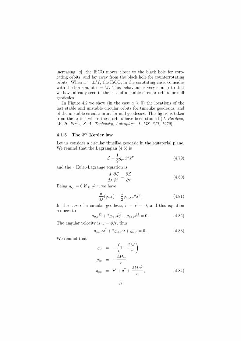
increasing |a|, the ISCO moves closer to the black hole for coro-tating orbits, and far away from the black hole for counterrotatingorbits. When a = ±M , the ISCO, in the corotating case, coincideswith the horizon, at r = M . This behaviour is very similar to thatwe have already seen in the case of unstable circular orbits for nullgeodesics.

In Figure 4.2 we show (in the case a ! 0) the locations of thelast stable and unstable circular orbits for timelike geodesics, andof the unstable circular orbit for null geodesics. This figure is takenfrom the article where these orbits have been studied (J. Bardeen,W. H. Press, S. A. Teukolsky, Astrophys. J. 178, 347, 1972).

4.1.5 The 3rd Kepler law

Let us consider a circular timelike geodesic in the equatorial plane.We remind that the Lagrangian (4.5) is

L =1

2gµ! x

µx! (4.79)

and the r Euler-Lagrange equation is

d

d!

"L"r

="L"r

. (4.80)

Being grµ = 0 if µ *= r, we have

d

d!(grrr) =

1

2gµ!,rx

µx! . (4.81)

In the case of a circular geodesic, r = r = 0, and this equationreduces to

gtt,r t2 + 2gt#,rt$+ g##,r$

2 = 0 . (4.82)

The angular velocity is * = $/t, thus

g##,r*2 + 2gt#,r* + gtt,r = 0 . (4.83)

We remind that

gtt = #!1# 2M

r

"

gt# = #2Ma

r

g## = r2 + a2 +2Ma2

r, (4.84)

82

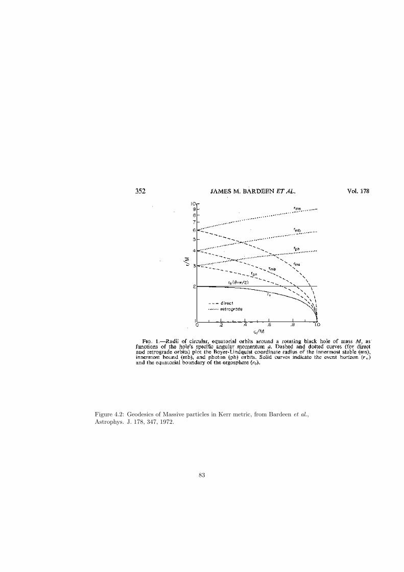
Figure 4.2: Geodesics of Massive particles in Kerr metric, from Bardeen et al.,Astrophys. J. 178, 347, 1972.

83

then

2

!r # Ma2

r2

"*2 +

4Ma

r2* # 2M

r2= 0 . (4.85)

The equation

(r3 #Ma2)*2 + 2Ma* #M = 0 (4.86)

has discriminant

M2a2 +M(r3 #Ma2) = Mr3 (4.87)

and solutions

*± =#Ma ±

$Mr3

r3 #Ma2= ±

$M

r3/2 ) a$M

r3 #Ma2

= ±$M

r3/2 ) a$M

(r3/2 + a$M)(r3/2 # a

$M)

= ±$M

r3/2 ± a$M

. (4.88)

This is the relation between angular velocity and radius of circularorbits, and reduces, in Schwarzschild limit a = 0, to

*± = ±*

M

r3, (4.89)

which is Kepler’s 3rd law.

4.2 General geodesic motion: the Carter con-stant

To study generic geodesics in Kerr spacetime, we need to applythe Hamilton-Jacobi approach, which allows to identify a furtherconstant of motion (not related to any isometry of the metric).

To apply the Hamilton-Jacobi approach, we first have to expressour system with an Hamiltonian description. Given the Lagrangianof the system

L(xµ, xµ) =1

2gµ! x

µx! (4.90)

84

we have defined the conjugate momenta2

pµ ="L"xµ

= gµ! x! . (4.91)

By inverting (4.91), we can express xµ in terms of the conjugatemomenta:

xµ = gµ!p! . (4.92)

The Hamiltonian is a functional of the coordinate functions xµ(!)and of their conjugate momenta pµ(!), defined as

H(xµ, p!) = pµ xµ(p!)# L (xµ, xµ(p!)) . (4.93)

In our case, we have

H =1

2gµ!pµp! . (4.94)

The geodesics equation is equivalent to the Euler-Lagrange equa-tions for the Lagrangian functional, which are equivalent to theHamilton equations for the Hamiltonian functional:

xµ ="H

"pµ

pµ = # "H

"xµ. (4.95)

To solve equations (4.95) is as di!cult as to solve the Euler-Lagrangeequations. Anyway, it is possible to apply the Hamilton-Jacobi ap-proach, which here we briefly recall.

In the Hamilton-Jacobi approach, we look for a function of thecoordinates and of the curve parameter !,

S = S(xµ,!) (4.96)

which is solution of the Hamilton-Jacobi equation

H

!xµ,

"S

"xµ

"+

"S

"!= 0 . (4.97)

In general such a solution will depend on four integration constants.It can be shown that, if S is a solution of the Hamilton-Jacobi

equation, then"S

"xµ= pµ . (4.98)

2Not to be confused with the four-momentum of the particle, which we denote with Pµ.

85

Therefore, once we have solved (4.97), we have the expressions ofthe conjugate momenta (and then of xµ) in terms of four constants,which allow to write the solutions of the geodesic equation in aclosed form, in terms of integrals.

In general, it is more di!cult to solve (4.97), which is a partialdi"erential equation, than to solve the geodesic equation, but in thiscase we can find such a solution.

First of all, we can use what we already know, i.e.

H =1

2gµ!pµp! =

1

2%

pt = #E constant

p# = L constant . (4.99)

These conditions require that

S = #1

2%!# Et+ L$+ S(r$)(r, &) (4.100)

where S(r$) is a function of r and & to be determined.Furthermore, we look for a separable solution, by making the

ansatz

S = #1

2%!# Et+ L$+ S(r)(r) + S($)(&) . (4.101)

Substituting (4.101) into the Hamilton-Jacobi equation (4.97), andusing the expression (3.16) for the inverse metric, we find

#% +$

#

!dS(r)

dr

"2

+1

#

!dS($)

d&

"2

# 1

$

%r2 + a2 +

2Mra2

#sin2 &

&E2 +

4Mra

#$EL+

$# a2 sin2 &

#$ sin2 &L2 = 0 .

(4.102)

Using the relation (3.12)

(r2 + a2) +2Mra2

#sin2 & =

1

#

'(r2 + a2)2 # a2 sin2 &$

((4.103)

and multiplying by # = r2 + a2 cos2 &, we get

#%(r2 + a2 cos2 &) +$

!dS(r)

dr

"2

+

!dS($)

d&

"2

86

#%(r2 + a2)2

$# a2 sin2 &

&E2 +

4Mra

$EL+

!1

sin2 &# a2

$

"L2 = 0

(4.104)

i.e.

$

!dS(r)

dr

"2

# %r2 # (r2 + a2)2

$E2 +

4Mra

$EL# a2

$L2

= #!dS($)

d&

"2

+ %a2 cos2 & # a2 sin2 &E2 # 1

sin2 &L2 .

(4.105)

We rearrange equation (4.105) by adding to both sides the constantquantity a2E2 + L2:

$

!dS(r)

dr

"2

# %r2 # (r2 + a2)2

$E2 +

4Mra

$EL# a2

$L2 + a2E2 + L2

= #!dS($)

d&

"2

+ %a2 cos2 & + a2 cos2 &E2 # cos2 &

sin2 &L2 .

(4.106)

In equation (4.106), the left-hand side does not depend on &, and itis equal to the right-hand side which does not depend on r; therefore,this quantity must be a constant C:

!dS($)

d&

"2

# cos2 &

%(%+ E2)a2 # 1

sin2 &L2

&= C

$

!dS(r)

dr

"2

# %r2 # (r2 + a2)2

$E2 +

4Mra

$EL# a2

$L2 + E2a2 + L2

= $

!dS(r)

dr

"2

# %r2 + (L# aE)2 # 1

$

'E(r2 + a2)# La

(2= #C .

(4.107)

Notice that in rearranging the terms between the last two lines, wehave used, for the LE terms, the relation

#2aLE + 2aLEr2 + a2

$=

4aMr

$LE . (4.108)

87

If we define the functions R(r) and &(&) as

&(&) " C + cos2 &

%(% + E2)a2 # 1

sin2 &L2

&

R(r) " $'#C + %r2 # (L# aE)2

(+'E(r2 + a2)# La

(2,

(4.109)

then!dS($)

d&

"2

= &

!dS(r)

dr

"2

=R

$2(4.110)

and the solution of the Hamilton-Jacobi equation has the form

S = #1

2%!#Et + L$+

) $R

$dr +

) $&d& . (4.111)

Once we have the solution of the Hamilton-Jacobi equations, de-pending on four constants (%, E, L, C), it is possible to solve thegeodesic motion. Indeed, from (4.98) we know the expressions ofthe conjugate momenta

p2$ = (#&)2 = &(&)

p2r =

!#

$r

"2

=R(r)

$2(4.112)

therefore

& = ± 1

#

$&

r = ± 1

#

$R (4.113)

which can be solved by simple integration. The constant C is calledCarter constant, and characterize, together with E and L, the geodesicmotion. Notice that di"erently from E and L, the Carter constantis not related to any isometry of the spacetime.

To integrate equations (4.113), it is convenient to define a newvariable !" to parametrize the geodesic, called “Mino time”:

d! = #d!" = (r2 + a2 cos2 &)d!" . (4.114)

88

Then we have

d&

d!" = ±+&(&)

dr

d!" = ±+

R(r) , (4.115)

thus the equations for r and &, once expressed in the Mino time, aredecoupled. An important consequence of this property is that forbound orbits, which satisfy R(r) > 0 for r1 < r < r2 and &(&) > 0for &1 < & < &2(= ' # &1), the functions r(!") and &(!") Are:

r(!") = r(!" + n'r)

&(!") = &(!" + k'$) (4.116)

with n, k integers and periods

'r = 2

) r2

r1

dr$R

'$ = 2

) $2

$1

d&$&

. (4.117)

The orbits, still, are very complicate, since the periods in r and &are di"erent, and t,$ are not periodic at all: a generic bound orbitdoes not resemble to an ellipse.

89