DECAY FOR SOLUTIONS OF THE WAVE EQUATION ON KERR …

DECAY FOR SOLUTIONS OF THE WAVE EQUATION

ON KERR EXTERIOR SPACETIMES I-II :

THE CASES ∣a∣ ≪M OR AXISYMMETRY

MIHALIS DAFERMOS AND IGOR RODNIANSKI

Abstract. This paper contains the first two parts (I-II) of a three-part se-ries concerning the scalar wave equation 2gψ = 0 on a fixed Kerr background

(M, ga,M ). We here restrict to two cases: (II1) ∣a∣ ≪ M , general ψ or (II2)

∣a∣ < M , ψ axisymmetric. In either case, we prove a version of ‘integratedlocal energy decay’, specifically, that the 4-integral of an energy-type density

(degenerating in a neighborhood of the Schwarzschild photon sphere and at

infinity), integrated over the domain of dependence of a spacelike hypersur-face Σ connecting the future event horizon with spacelike infinity or a sphere

on null infinity, is bounded by a natural (non-degenerate) energy flux of ψ

through Σ. (The case (II1) has in fact been treated previously in our ClayLecture notes: Lectures on black holes and linear waves, arXiv:0811.0354.)

In our forthcoming Part III, the restriction to axisymmetry for the general∣a∣ < M case is removed. The complete proof is surveyed in our companion

paper The black hole stability problem for linear scalar perturbations, which

includes the essential details of our forthcoming Part III. Together with pre-vious work (see our: A new physical-space approach to decay for the wave

equation with applications to black hole spacetimes, in XVIth International

Congress on Mathematical Physics, Pavel Exner ed., Prague 2009 pp. 421–433, 2009, http://arxiv.org/abs/0910.4957), this result leads, under suitable

assumptions on initial data of ψ, to polynomial decay bounds for the energy

flux of ψ through the foliation of the black hole exterior defined by the timetranslates of a spacelike hypersurface Σ terminating on null infinity, as well as

to pointwise decay estimates, of a definitive form useful for nonlinear applica-

tions.

Contents

1. Introduction 31.1. Overview 31.2. Statement of the main theorems 81.3. Other decay-type statements 121.4. Related spacetimes and equations 132. The Kerr spacetime 132.1. The fixed manifold-with-boundary R 132.2. Kerr-star coordinates 132.3. The coordinate r∗ 142.4. Boyer-Lindquist coordinates 142.5. The Kerr metric 152.6. The Carter-Penrose diagramme 16

Date: October 24, 2018.

1

arX

iv:1

010.

5132

v1 [

gr-q

c] 2

5 O

ct 2

010

http://arxiv.org/abs/0811.0354


2 MIHALIS DAFERMOS AND IGOR RODNIANSKI

2.7. The event horizon H+ as a Killing horizon 162.8. Asymptotics and angular momentum operators 172.9. The volume form 173. The geometry of Kerr 173.1. Surface gravity and the redshift 183.2. The ergoregion and superradiance 183.3. Separability of geodesic flow and trapped null geodesics 204. Preliminaries 214.1. Generic constants and fixed parameters 214.2. Vector field multipliers and commutators 214.3. Hardy inequalities 224.4. Admissible hypersurfaces 224.5. Well-posedness 234.6. A reduction 244.7. Uniform boundedness 245. A JN multiplier current and the red-shift 255.1. The construction of N 255.2. The red-shift estimate 265.3. The red-shift vs. superradiance 265.4. Red-shift commutation 285.5. The higher order statement 286. A current for large r 297. Separation 307.1. Oblate spheroidal harmonics 307.2. Carter’s separation 327.3. Basic properties of the decomposition 328. Cutoffs 339. The frequency localised multiplier estimates 349.1. The separated current templates 349.2. The frequency ranges 359.3. The F range (bounded frequencies) 359.4. The F range (angular dominated frequencies) 419.5. The F range (trapped frequencies) 429.6. The F♯ range (time-dominated frequencies) 4510. Summing 4610.1. The main term 4610.2. Error terms near the horizon and infinity 4710.3. Error terms from the cutoff 4710.4. Boundary terms 5010.5. Finishing the proof 5011. Acknowledgements 51Index 52References 54

DECAY FOR SOLUTIONS OF THE WAVE EQUATION ON KERR I-II 3

1. Introduction

The Kerr metrics gM,a constitute a remarkable two-parameter family of explicitsolutions to the Einstein vacuum equations

(1) Rµν = 0

and describe spacetimes corresponding to rotating stationary black holes with massM and angular momentum aM , as measured at infinity.

The family was discovered in local coordinates in 1963 by Kerr [53], and withinthe subsequent decade, its salient local and global geometric features were defini-tively understood, especially through work of Carter [16]. It is widely expectedthat the exterior region of the Kerr family is dynamically stable in the context ofthe Cauchy problem (see [21]) for (1), in fact, that for a wide range of initial datafor (1), not necessarily close to data arising from gM,a, the solution metric g inan appropriate region asymptotically settles down to a member of the family. Seethe discussion in [56]. Indeed, it is this expectation which lies at the basis for thecentrality of the Kerr metric in our current astrophysical world-view. At present,however, a mathematical resolution of even the stability question (i.e. the dynamicsfor spacetimes g initially very near gM,a) remains a great open problem in classicalgeneral relativity. Many of the important difficulties of this problem are alreadymanifest at the linear level, for the conjectured stability mechanism would rest fun-damentally on the dispersive properties of waves (an essentially linear phenomenon)in the black hole exterior region. One must certainly address, thus, the followingcentral mathematical question:

Do waves indeed disperse on Kerr backgrounds, and how does one properlyquantify this?

1.1. Overview. Motivated by the above, we consider the scalar homogeneous waveequation

(2) 2gψ = 0

on exactly Kerr spacetimes (M, gM,a). The study of (2) can be thought of as apoor-man’s linear theory associated to (1), neglecting, in particular, its tensorialstructure. For results pertinent to the latter, see Holzegel [51]. In the presentpaper, we shall restrict to either of the following cases:

The parameters of the Kerr metric satisfy ∣a∣ ≪M . The parameters of the Kerr metric are allowed to lie in the entire subex-

tremal range ∣a∣ <M , but ψ is assumed axisymmetric.

The significance of the restriction ∣a∣ ≪M is that the effect of superradiance (to bediscussed below) is weak, and this weakness can be exploited as a small parameter.In the axisymmetric case, superradiance is in fact entirely absent. A forthcomingpaper [39] will consider non-axisymmetric solutions for the general subextremalcase ∣a∣ <M , thus completing the study of the problem at hand. We provide in ourcompanion paper [38] the essential details of the proof in [39].

(Note: Part I of the present paper (consisting of Sections 1–7) alreadyprovides certain preliminary results relevant to the entire series. Withthe completion of Part III, Part I will be further extended so as to serveas an introduction to the entire series and will be broken off from part


II (Sections 8–10), which will retain the proofs in the cases (II1), (II2)above.)

1.1.1. Boundedness. The most primitive global question concerning solutions to(2) which one must address is that of boundedness. The essential difficulty ofthis problem lies in the phenomenon of ‘superradiance’. Briefly put, superradiancemeans that, since the stationary Killing field T becomes spacelike at some pointsof the exterior region for all Kerr spacetimes with ∣a∣ ≠ 0, the energy radiated toinfinity can be greater than the initial energy on a Cauchy hypersurface. In fact, itis not a priori obvious that the energy radiated to infinity (and hence the solutionpointwise, etc.) can be controlled at all.

This long-standing open problem of energy and pointwise boundedness has beenresolved previously in our [35] for solutions to (2) on a general class of axisymmetric,stationary black hole exterior spacetimes sufficiently close to the Schwarzschildmetric, a class which includes as a special case the Kerr family gM,a for ∣a∣ ≪ M ,as well as the Kerr-Newman family gM,a,Q for ∣a∣ ≪M , ∣Q∣ ≪M .

Recall that the Schwarzschild family, discovered already in 1916, is precisely thesubfamily of Kerr correponding to a = 0. For the Schwarzschild case, superradianceis absent as the stationary Killing field T is in fact non-spacelike everywhere in theexterior. Thus, the boundedness statement is much easier, though still non-trivialif one desires uniform control up to the horizon where T becomes null; for this,results go back to Wald [85] and Kay–Wald [52]. See the discussion in [36] formany further references.

The fact that under the assumptions of [34], superradiance is weak and can betreated as a small parameter is fundamental for the boundedness proof. It is in factmore natural to discuss briefly the strategy of this proof in the following section,after discussing some of the ideas involved in proving decay, in particular becausethe main theorem of the present paper will retrieve the boundedness statement inthe special case of the Kerr family with ∣a∣ ≪M .

We note finally that boundedness for axisymmetric solutions of (2) on Kerrexteriors in the entire subextremal range ∣a∣ < M also follows from [35]. Thislatter case shares the feature with Schwarzschild that superradiance is absent, asthe energy defined by T is nonnegative definite in the exterior when restricted toaxisymmetric ψ.

1.1.2. Integrated local energy decay. The present paper thus concerns the problemof decay for ψ precisely in the cases for which boundedness was previously known.Our main theorems (Theorem 1.1 and 1.2 below) state that, for the two casesoutlined above:

The spacetime integral of an energy-type density integrated over the domainof development of an appropriate surface Σ is bounded by an initial energy-type flux through Σ (see (4)).

The above spacetime energy density is non-degenerate at the horizon, but degener-ates at infinity and in a region to which “trapped null geodesics” (see Section 3.3)approach. Both these degenerations are necessary. The boundedness of a spacetimeintegral degenerating only at infinity can then be obtained (see (7)) in terms of ahigher order initial energy type quantity. Estimates (4) and (7) should be thoughtof as statements of dispersion which often go by the name “integrated local energydecay”.


Let us briefly put these results in perspective. In Minkowski space, the analogueof estimate (4), with degeneration only at infinity, was first shown in seminal workof Morawetz [69], via use of an identity associated to a virial-type current. In thatcase, the analogous estimate applied to Σ = t = 0 would take the form

(3) ∫R4

(1+r)−1−δ∣∂tψ∣

2+(1+r)−1−δ

∣∂rψ∣2+r−1

∣∇/ψ∣2 ≤ Cδ ∫t=0

∣∂tψ∣2+ ∣∂rψ∣

2+ ∣∇/ψ∣2.

for any δ > 0, where r is a standard spherical coordinate and ∇/ denotes the inducedgradient on the constant (r, t) spheres. Such estimates were extended to solutionsof the wave equation outside of non-trapping obstacles in [70]. On the other hand,it was shown by Ralston [76] that in the presence of trapping, the integrand of theleft-hand side of such an estimate must degenerate near trapped rays. Analoguesof (4) in the Schwarzschild case a = 0, exhibiting for the first time the expecteddegeneration associated with the photon sphere of trapped null geodesics (see Sec-tion 3.3), were pioneered by [60, 11], with unnecessary additional degeneration onthe horizon, however. This degeneration was related to the fact that naively, thenull generators of the horizon may seem to be subject to the trapping obstructionof Ralston, if one does not remark that their tangent vectors shrink exponentiallywith respect to the stationary Killing field. This is essentially the redshift effect.The degeneration at the horizon was then overcome in [32] by using a new vectorfield multiplier current which quantifies this celebrated effect. As we shall see, thisis essential for the stability of the construction. Analogues of (4), (7) for a = 0 haveby now been obtained, extended and refined by many authors [32, 12, 34, 2, 13, 64].See [36] for a detailed review.

In passing from Schwarzschild to Kerr, two major difficulties appear immediately.One is the superradiance effect mentioned earlier, the other is the more complicatedstructure of trapped null geodesics. In view of the previous work described justabove in Section 1.1.1, the former difficulty has been completely resolved in thecases under consideration. The latter difficulty was beautifully expounded upon byAlinhac [2], who explicitly showed that currents of the form of [32] can never yieldnonnegative definite spacetime estimates on Kerr spacetimes for ∣a∣ ≠ 0, even inthe high frequency approximation; this is essentially related to the fact that thereare trapped null geodesics for an open range of r, whereas the construction of thecurrents of [32] implicitly rely on the fact that in Schwarzschild, all such geodesicsapproach the codimension-1 hypersurface r = 3M .

It turns out that the “exceptionalism” of Schwarzschild from this point of view isin some sense merely an accident of the projection of geodesic flow to the spacetimemanifold. On the tangent bundle, the dynamics of geodesic flow near trapped nullgeodesics is stable upon passing from a = 0 to ∣a∣ ≪ M . This stability is in turnrelated to the separability and thus complete integrability of geodesic flow for Kerrmetrics, first discovered by Carter [17].

The geometric origin of the separability of geodesic flow is subtle. Besides Killingfields T and Φ, the Kerr geometry admits a nontrivial independent Killing ten-sor [86]. It turns out that using the Ricci flatness, this implies both separabilityof geodesic flow and separability of the wave equation [18]. The latter provides aconvenient way to frequency-localise the virial currents JX,w of [32, 12] and subse-quent papers, in a way intimately tied to both the local and global geometry of thesolution. This localisation allows us to capture the obstruction to integrated decayprovided by trapped null geodesics, overcoming the difficulty described in [2].


The properties of geodesic flow are only suggestive of the high frequency regimeof solutions ψ of (2). To retrieve the original spacetime integral estimates proven inthe Schwarzschild case with the Morawetz-type current, one must understand thebehaviour of such currents on all frequencies, including low frequencies outside ofthe “trapped” regime. For the case ∣a∣ ≪M , one can essentially infer positivity bystability considerations from the previous constructions on Schwarzschild. In thegeneral case ∣a∣ <M , however, the existence of suitable currents providing positivitywould depend on global geometric features of the Kerr metric. The geometricfrequency-localisation we have employed is particularly suitable for exploiting this.This is all the more important to make contact with our forthcoming part III [39],where low frequencies in the non-trapped but superradiant regime introduce a newimportant difficulty. See the discussion in our companion paper [38].

It is perhaps useful at this point to recall how boundedness was proven in [35] forthe wave equation on suitable axisymmetric, stationary perturbations of Schwarz-schild. After applying appropriate cutoffs and taking Fourier expansions associatedto the Killing directions T and Φ, one can partition general solutions into theirsuperradiant and non-superradiant part, where the latter part is distinguished bythe positivity of its energy flux through the horizon. The crucial observation isthat for sufficiently small perturbations of Schwarzschild space, the superradiantpart is non-trapped, and a Morawetz-type current could be constructed withoutdegeneration, essentially from the original Schwarzschild construction and stabilityconsiderations. Adding, a small part of the ‘red-shift vector field’ component of thecurrent as first introduced in [32], and in addition, the stationary Killing vector fieldT , the boundary terms of this current could also be shown to be positive, withoutdestroying the positivity of the spacetime integral. This observation (together witha new robust argument to show boundedness in the case where the energy flux ispositive through the horizon) was sufficient to prove boundedness for the sum ofthe superradiant and non-superradiant part.

Turning back to the problem at hand, in view of the fact that boundedness hasalready been proven, we need not worry here about the sign of boundary terms inour construction. Of course, the observation due to [32] that the boundary termscan be made positive by adding a small amount of the red-shift current can be ap-plied directly here. Thus, the proof of Theorem 1.1 in fact reproves the boundednessstatement, when specialised to the case of Kerr spacetimes with ∣a∣ ≪ M , and wehave indeed set things up so that the boundedness statement (see (11)) is retrievedrather than used. This emphasizes a philosophical point: when superradiance issmall, one need not distinguish the superradiant part from the nonsuperradiantpart, provided one is indeed proving dispersion for the total solution. This distinc-tion, however, is an important aspect of the general non-axisymmetric case ∣a∣ <M .In particular, as in the general boundedness theorem [35], it is essential to constructmultipliers separately for the superradiant and non-superradiant regimes. See thediscussion in Section 5.3. These constructions are already given in detail in Section11 of our companion paper [38].

1.1.3. Red-shift commutation and higher derivatives. Non-linear applications makeit imperative to understand boundedness and decay properties for higher orderquantities. In the usual application of the vector field method, these are typicallyproven via commutation with Killing fields, or, on dynamical geometries, vectorfields which become Killing asymptotically in time. It is here essential that the


set of commutators span a timelike direction, so that all derivatives can then berecovered by elliptic estimates.

Already in the Schwarzschild case, one is faced with the difficulty that the span ofthe Killing fields does not include a timelike direction at points on the event horizon.This difficulty was circumvented by Kay and Wald in their celebrated [52] for thepurpose of proving pointwise estimates for ψ itself on the horizon. Unfortunately,the method of [52] was very fragile. In addition, the method was not able, forinstance, to uniformly bound transversal (to the horizon) derivatives of ψ.

It was first shown in the context of our general boundedness theorem of [35],referred to above, that commutation by a suitable transverse vector field to thehorizon, though not Killing, has the property that the most dangerous error termswhich arise have a favourable sign. This is yet another manifestation of the redshift,and, as shown in Section 7 of [36], is in fact true for all Killing horizons with positivesurface gravity. Using this commutation, one can obtain higher order decay resultswhich do not degenerate at the horizon. We have included these statements in ourresults. See Theorem 1.3.

1.1.4. Further decay. On the surface, the local integrated decay statement of The-orems 1.1 and 1.2 appears to be a very weak statement of dispersion, seeminglyfar from the type of statements necessary to obtain non-linear stability results asin [25]. It turns out, however, that it is the essential ingredient in obtaining furtherdecay.

This fact was already partially apparent from work in the Schwarzschild case.In addition to proving a version of Theorem 1.1 for a = 0 incorporating for the firsttime a vector field estimate capturing the red-shift effect, our [32] gave a method forthen inferring quantitative decay of energy through a suitable foliation, through useof a suitably constructed conformal Morawetz multiplier. Independently, a relatedargument was developed in [14]. The construction of the conformal Morawetzmultiplier appeared however to still be sensitive to the global geometry all the wayup to the event horizon. In [37] and our companion [40], however, it is shown that fora wide class of metrics, (i) a local integrated decay statement as in Theorem 1.1, (ii)a uniform boundedness statement as in [35], and (iii) an additional estimate whosevalidity depends only on the asymptotic behaviour of the metric at null infinity aretogether in fact sufficient to prove quantitative decay of energy (through a suitablefoliation) and pointwise decay of the form useful for non-linear stability problems.We note that this argument has other potential applications unrelated to the blackhole case. In particular, one need not assume the metric to be stationary (or evenasymptotically stationary as t→∞; see the recent nonlinear application of [88]). Itis fundamental, however, that the local energy decay statement be nondegenerateat horizons, if the latter are present. For completeness, we will include in this papera version of the resulting decay estimates (Theorem 1.4) for the Kerr case. In thiscontext, we note also an independent Fourier based method of obtaining refinedpointwise decay estimates [81] from Theorem 1.1, relying heavily however on exactstationarity.

1.1.5. Final remarks. A version of Theorem 1.1 and its proof first appeared asProposition 5.3.1 of our Clay lecture notes [36], where, in addition, an earliermethod for turning this into energy and pointwise decay (Theorem 5.2), closelyfollowing [32], was also presented. The original method of proof of Theorem 5.2


has been extended to yield additional decay on Kerr by Luk [63] via commutationby the scaling vector field, following a method he introduced in the Schwarzschildcase [62]. Furthermore, this additional decay is then used in [63] to obtain a stabil-ity result for the wave-map equation on Kerr for ∣a∣ ≪M . Note that this additionaldecay is also retrieved in the statement of Theorem 1.4 and its corollaries.

We give here a new proof of Theorem 1.1 in order (i) to give a self-containedpresentation in paper form not depending on the previous delicate constructionson Schwarzschild (see [32, 12, 34] and subsequent papers), (ii) to unify it with theproof of Theorem 1.2 which appears here for the first time, and in addition, (iii) tointroduce constructions and notations which will be used in the forthcoming PartIII [39] concerning the case of non-axisymmetric solutions for the general parameterrange ∣a∣ <M . See also our companion [38] which gives a complete survey, includingthe essential details of the constructions of [39].

We mention finally that in parallel with the results of [36] concerning decay, thereare two independent other approaches to the problem for ∣a∣ ≪M which have sinceappeared, due to Tataru–Tohaneanu [82], and, more recently, Andersson–Blue [3].The former replaces frequency localisation via Carter’s separation with a techniquebased on the standard pseudo-differential calculus, whearas the latter introducesan innovative alternative technique for frequency localisation via commutation byhigher order operators related to the Killing tensor, but requires a high degree ofregularity and fast decay of initial data near spatial infinity. Another importantrelated development is due to Tohaneanu [83], who, starting from integrated decayestimates in [82], shows Strichartz estimates with nice applications to semi-linearproblems.

1.2. Statement of the main theorems.

1.2.1. Notations. The statement of the main theorem will depend on a number ofdefinitions and notations, which we briefly summarise here. These notions will bedeveloped formally further in the paper.

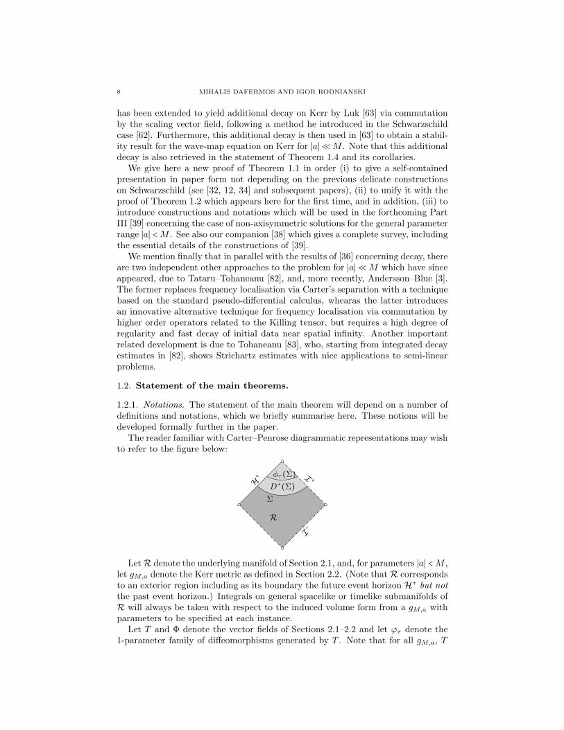
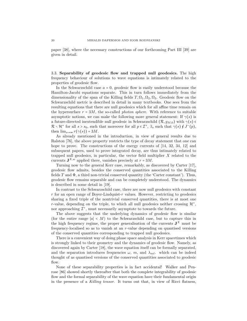
The reader familiar with Carter–Penrose diagrammatic representations may wishto refer to the figure below:

R

H+ I +

I−

Σ

φτ(Σ)D+(Σ)

LetR denote the underlying manifold of Section 2.1, and, for parameters ∣a∣ <M ,let gM,a denote the Kerr metric as defined in Section 2.2. (Note that R correspondsto an exterior region including as its boundary the future event horizon H+ but notthe past event horizon.) Integrals on general spacelike or timelike submanifolds ofR will always be taken with respect to the induced volume form from a gM,a withparameters to be specified at each instance.

Let T and Φ denote the vector fields of Sections 2.1–2.2 and let ϕτ denote the1-parameter family of diffeomorphisms generated by T . Note that for all gM,a, T


will correspond to the stationary Killing field, and Φ will correspond to the Killingfield generator of axisymmetry.

We will in general consider the class of so-called “admissible” hypersurfaces, to bedefined in Section 4.4. The definition of admissibility depends on the parametersM > a0, and applies for all metrics gM,a with ∣a∣ ≤ a0. What is depicted in thediagramme is an admissible hypersurface “of the second kind”.

The following notions will depend on the metric ga,M , i.e. on both the parameters∣a∣ <M chosen: Let r denote the coordinate of Section 2.2. Let Z∗ denote the uniquesmooth extension toR of the coordinate vector field ∂r defined with respect to Kerr-star coordinates, whereas let Z denote the unique smooth extension to int(R) of ∂rdefined with respect to Boyer-Lindquist coordinates (see Section 2.4). Note that Z∗

is transverse to H+, whereas Z would not extend smoothly to H+. Note also thatfor ∣a∣ ≪M , we have Z∗ = Z in r ≥ 5M/2, by our definition of Kerr star cordinates.Let N denote the vector field of Section 5. This is a timelike, ϕτ -invariant vectorfield transverse to H+, which coincides with T identically sufficiently far from the

horizon. Let r+ denote the limiting value of r on H+, r+ =M +√M2 − a2. Let g/, ∇/

denote the induced metric and covariant derivative from ga,M on the S2 factors ofR in the differential-topological product (13). For a general spacelike hypersurfaceΣ ⊂ R, we let nΣ denote the unit future normal. Let D+(Σ) denote the futuredomain of dependence of Σ in R. Finally, for a general vector field V , let JV [ψ]denote the 1-form ‘energy’ current defined in Section 4.2.

1.2.2. The statement for ∣a∣ ≪M .

Theorem 1.1. Fix M > 0. There exists a constant ε = ε(M) > 0 such that for all0 ≤ a0 ≤ ε, the following statement holds:

There exist smoothly depending positive values s±(a0,M) with with s±(0,M) = 0such that the following holds. Let Σ be an arbitrary admissible hypersurface in R(of the first or second kind) for parameter M . Then, for all δ > 0, there existsa constant B = B(Σ, δ) = B(ϕτ(Σ), δ) such that for all ∣a∣ ≤ a0, considering themetric gM,a on R, r+ < 5M/2 < 3M − s−, and such that for all sufficiently regularsolutions ψ of (2) with g = gM,a on D+(Σ), the following inequalities hold (allmetric dependent quantities referring to g = gM,a, as described above) for ψ

∫D+(Σ)

(r−1(1 − η[3M−s−,3M+s+])(1 − 3M/r)2(∣∇/ψ∣2 + r−δ((Tψ)2))

+r−1−δ(Z∗ψ)2 + r−3−δ(ψ − ψ∞)2)(4)

≤ B ∫Σ JNµ [ψ]nµΣ,

(5) ∫ϕτ (Σ)

JNµ [ψ]nµΣ ≤ B ∫Σ

JNµ [ψ]nµΣ, ∀τ ≥ 0,

(6) ∫H+∩D+(Σ)JNµ [ψ]nµH+ + (ψ − ψ∞)

2≤ B ∫

ΣJNµ [ψ]nµΣ,

where 4πψ2∞ = limr′→∞ ∫Σ∩r=r′ r

−2∣ψ∣2, and η denotes the indicator function.

The term ‘sufficiently regular’ above just means solutions of 2gψ on D+(Σ) such

that on any compact spacelike hypersurface-with-boundary Σ ⊂ D+(Σ), then ψ

and nΣψ have well-defined traces on Σ which are in H1loc(Σ), L2

loc(Σ) respectively.There exists a unique such solution for appropriately defined initial data along Σ.


See Section 4.5. Note that under these regularity assumptions, ψ∞ is well definedand is finite if the right hand side of (4) is finite.

Statement (4) is the analogue for Kerr of Morawetz’s estimate (3) for Minkowskispace and the integrated decay estimate of [32] for Schwarzschild. The inclusionof the (1 − 3M/r)2 factor is so as to obtain uniform constants as a0 → 0, so as toretrieve in particular the Schwarzschild result, for which Theorem 1.1 provides infact an independent proof.

Let us note that (5) followed from our previous boundedness theorem of [35],when the statement of the latter is restricted to the Kerr family. As discussedabove, our theorem gives an independent proof of this statement in the Kerr case.The theorem of [35] also gave an inequality similar to but weaker than (6), withJNµ [ψ]nµH+ replaced by ∣JTµ [ψ]n

µH+ ∣ and without the 0’th order term.

We note immediately:

Corollary 1.1. Under the assumptions of the above theorem,

(7) ∫D+(Σ)

r−1−δJNµ [ψ]Nµ+ r−3−δ

(ψ − ψ∞)2≤ B ∫

Σ(JNµ [ψ] + JNµ [Tψ])nµΣ.

Let us note finally that the proof in fact yields an estimate for solutions to theinhomogeneous equation

(8) 2gψ = F,

which we here omit for reasons of brevity.

1.2.3. The statement for axisymmetric solutions. Our second main theorem of thepresent paper concerns the entire subextremal range ∣a∣ < M but is restricted toaxisymmetric solutions.

Theorem 1.2. Fix M > 0. Then for each 0 ≤ a0 <M , δ > 0, and each Σ admissiblefor a0, M , then for all ∣a∣ ≤ a0, there exist values s±(a), with r+(a,M) < 3M −s−, aconstant B = B(a0, δ,Σ), and a cutoff function χa(r), with χa = 1 for r ≥ 3M − s−

and χa = 0 for r ≤ (r+ + 3M − s−)/2, such that defining Z∗ = χaZ + (1−χa)Z∗, then

the following statement holds.For all ∣a∣ ≤ a0, and all sufficiently regular solutions ψ of (2) with g = gM,a on

D+(Σ), which moreover satisfy

(9) Φ(ψ) = 0,

the inequalities (4)–(7) hold, with Z∗ in place of Z∗.

The restriction (9) is removed in our companion paper [39].A posteriori, we note that one could have defined Kerr star coordinates so as

for the distinction between Z∗ and Z∗ to be unnecessary, but this would requiremaking the definition depend on certain constants that only appear in the proof ofour theorem.

1.2.4. The higher order statement.

Theorem 1.3. Let M , a0, a, gM,a, s±, ψ be as in Theorem 1.1 or 1.2.


Then, for all δ > 0 and all integers j ≥ 1, there exists a constant B = B(Σ, δ, j) =B(ϕτ(Σ), δ, j) such that the following inequalities hold (all metric dependent quan-tities referring to g = gM,a, as described above) for ψ

∫D+(Σ)

r−1−δ(1 − η[3M−s−,3M+s+])(1 − 3M/r)2∑1≤i1+i2+i3≤j ∣∇/

i1T i2(Z∗)i3ψ∣2

+r−1−δ∑1≤i1+i2+i3≤j−1 (∣∇/

i1T i2(Z∗)i3+1ψ∣2 + ∣∇/i1T i2(Z∗)i3ψ∣2)

≤ B∑0≤i≤j−1 ∫Σ JNµ [N iψ]nµΣ,(10)

∫ϕτ (Σ)

∑1≤i1+i2+i3≤j

∣∇/i1T i2(Z∗

)i3ψ∣2 ≤ B ∑

0≤i≤j−1∫ϕτ (Σ)

JNµ [N iψ]nµΣ

≤ B ∑0≤i≤j−1

∫Σ

JNµ [N iψ]nµΣ, ∀τ ≥ 0(11)

(12) ∑1≤i1+i2+i3≤j+1,i3≤j

∫H+∩D+(Σ)∣∇/i1(ni2H+N

i3ψ)∣2g/≤ B ∑

0≤i≤j−1∫

ΣJNµ [N iψ]nµΣ,

where again, Z∗ should be replaced by Z∗ in the case of Theorem 1.2.

For given fixed j ≥ 1, the regularity assumption on ψ implicit in the above state-ment is that on any compact spacelike hypersurface-with-boundary Σ ⊂ D+(Σ),

then ψ and nΣψ have well-defined traces on Σ which are in Hjloc(Σ), Hj−1

loc (Σ)

respectively.Note that the first line of (11) is simply an elliptic estimate whereas the second

asserts uniform boundedness of non-degenerate higher order energies. Again, (11)in the case of the assumptions of Theorem 1.1 followed from our previous bound-edness theorem of [35], when the statement of the latter is restricted to the Kerrfamily.

1.2.5. The statement of further decay. In view of Theorem 1.1 and the resultsof [37, 40], we may obtain further decay estimates, precisely of the form in principlecompatible with non-linear applications.

We give here only an example of the type of statement that can be shown. Theformulation of the result will require expanding the set of multiplier and commuta-tor vector fields: Let Ωi, i = 1,2,3, denote a set of angular momentum operators forthe ambient Schwarzschild metric gM (see Section 2.8), let L denote the outgoingnull vector

L =ρ2

√∆(ρ2 − 2Mr)

T +Z

and let L = χL where χ = 0 for r ≤ 3M say, and χ = 1 for r ≥ 5M . We have

Theorem 1.4. Under the assumptions of the above theorems and Σ an admissiblehypersurface of the second kind, then there exists a constant B = B(Σ) = B(φτ(Σ)),and, for each δ > 0 a constant Bδ = B(Σ, δ) = B(φτ(Σ), δ), such that for all suffi-ciently regular solutions ψ of (2) on D+(Σ),

∫ϕτ (Σ)

JNµ [ψ]nµϕτ (Σ) ≤ B τ

−2∑

0≤k≤2∫

ΣJN+r2Lµ [T kψ],

∫ϕτ (Σ)

JNµ [Nψ]nµϕτ (Σ) ≤ Bτ

−4+δ∑

i1+i2≤1

∑0≤k≤2

3

∑`=1∫

Σ(JN+r2Lµ [N i1Ωi2l T

kψ]+JN+r4−δLµ [T kLψ])nµΣ


Note that the above statement, together with a re-application of Theorem 1.1–applied now with Σ replaced by φτ(Σ), yields decay results (in τ) for spacetimeintegral on the left hand side of (4). This type of statement is in fact used in thecourse of the proof of Theorem 1.4.

From the above results, applied to ψ, Tψ, etc., and standard application ofthe vector field method, elliptic estimates, Sobolev inequalities, together with theadditional red-shift commutation of Section 5.4, one can obtain pointwise decayresults of the form:

Corollary 1.2. Under the assumptions of the above, we have

supϕτ (Σ)

r∣ψ − ψ∞∣ ≤ B√E τ−1/2,

supϕτ (Σ)∩r≤R

∣ψ − ψ∞∣ ≤ BR,δ√Eτ−3/2+δ,

supϕτ (Σ)∩r≤R

∣JNµ [ψ]Nµ∣ ≤ BR,δEτ

−4+δ,

where in each inequality, E denotes an appropriate quadratic integral quantity de-fined on Σ.

All these estimates have extensions to arbitrary derivatives of the solution (ofarbitrary order), including derivatives transverse to the horizon.

From the point of view of applications to quasilinear problems, past experiencewould suggest that the above type of results should be viewed as the definitivestatements of decay (cf. the role of decay results in the stability of Minkowskispace [25]). Less decay may not be enough to absorb error terms in stability proofs,whereas more refined decay statements (e.g. the familiar Price law tails from thephysics literature, see [29]), requiring of course more restrictive assumptions ondata, are potentially unstable in the context of the dynamical geometries of interest,and in any case, do not yield any added benefit for non-linear stability proofs.

In fact, it is immediate from the identity of Proposition 5.1.1 extended (simply bycontinuity!) to a region r ≥ r+ − ε(a,M), that any boundedness and suitable decayresult holding uniformly up to the horizon is propagated for instance to r+ − ε.More interestingly, this observation (first due to [28]) is stable in the consequenceof dynamical spacetimes where the event horizon and apparent horizon do not ingeneral coincide. The interesting question for black hole interiors is not, however,one of stability, but instability as one approaches the Cauchy horizon. This problemhas a long tradition of study: see [74] and [27, 28] in the context of the Einstein-Maxwell-scalar field system under spherical symmetry. (In the Kerr solution, theCauchy horizon corresponds to a hypersurface r = r− in maximally extended Kerr.)Further discussion of the behaviour ψ in the black hole interior is thus best left tosuch a context.

1.3. Other decay-type statements. There are many other important statements(mode stability, some partial nonquantitative results on azimuthal modes) whichhave appeared in the literature, at various levels of rigour. As a representativesample, we mention [87, 75, 48, 43, 44]. See our [36] for a discussion of this literature.


1.4. Related spacetimes and equations. We note finally that there has alsobeen interesting work on the Dirac equation [42, 47] on Kerr backgrounds, forwhich superradiance does not occur, and the Klein-Gordon equation in [8, 46], inthe case of non-superradiant modes. In the Schwarzschild case, there are a numberof papers on related equations. We note especially the work of Blue [10] on theMaxwell equations.

All questions considered have analogues in higher dimensions. For the waveequation on higher dimensional Schwarzschild, Schlue [79] has recently obtainedboth integrated energy decay and decay bounds for the energy flux and the solutionpointwise. See also [61].

When a cosmological constant Λ is added to the Einstein equations to give

Rµν = Λgµν ,

there corresponds a related family of solution spacetimes, which in the case Λ > 0is known as Kerr-de Sitter, whereas in the case Λ < 0 is known as Kerr-anti deSitter. For the Λ > 0 case, results have been obtained for the Schwarzschild-deSitter subcase by [33, 15] and recently extended in [65, 66]. Putting together themethods described here with [33] should yield a generalisation to the Kerr-de Sittercase for small a, but it would be nice to work this out explicitly. In the case ofKerr-anti de Sitter, we note the recent work of Holzegel [50].

2. The Kerr spacetime

2.1. The fixed manifold-with-boundary R. Let R denote the manifold withboundary

(13) R = R+×R × S2.

We define standard coordinates y∗ for R+, t∗ for R, and standard spherical coor-dinates (θ∗, φ∗) . Strictly speaking, the latter is only a coordinate system on thesubset of S2 corresponding to (0, π) × (0,2π), but we shall extend these functionsand the associated coordinate vector fields to all of S2, in the usual fashion.

The collection (y∗, t∗, θ∗, φ∗) define a coordinate system on R, global modulothe degeneration of the spherical coordinates remarked upon above. We will referto these as fixed coordinates.

Let us introduce the notation H+ = ∂R = y∗ = 0. We will refer to H+ as theevent horizon.

Let us denote T = ∂t∗ , Φ = ∂φ∗ , where, as remarked above, the latter is to beunderstood as the extension of the coordinate vector field to all of S2 in the usualway.

Let ϕτ denote the one-parameter family of diffeomorphisms generated by T .We have defined fixed coordinates precisely so that the differential structure of

the ambient spacetimesR, the vector fields which are to be Killing, and the locationof the horizon, are all independent of the Kerr parameters to be introduced in whatfollows.

2.2. Kerr-star coordinates. Let P ⊂ R2 denote the subset (x1, x2) ∶ 0 ≤ x1 <

x2. Define a smooth map

r ∶ P × (0,∞)→ (x2 +

√

x22 − x

21,∞)


such that r∣(x1,x2)×(0,∞) is a diffeomorphism (0,∞) → (x2 +√x2

2 − x21,∞) which

moreover restricts to the identity map restricted to (x1, x2) × (3x2,∞).Now, for each fixed parameters 0 ≤ a <M , the collection (r(a,M, y∗), t∗, θ∗, φ∗)

determines a coordinate system on R, global modulo the well-known degenerationof the spherical coordinates on S2. These will be known as Kerr-star coordinates.In what follows, we shall denote r(a,M, y∗) simply as r. As opposed to our fixedcoordinates on R, this latter coordinate depends on the parameters, although inthe region y∗ ≥ 3M , then r = y∗ and is thus independent of parameter a. Thecoordinate vector fields ∂t∗ and ∂φ∗ of Kerr-star coordinates always correspond tothe coordinate vector fields of the original fixed coordinate system, i.e. for all a,Mwe have ∂t∗ = T , ∂φ∗ = Φ.

Let us define

r± =M ±√M2 − a2;

note that these are smooth functions of the parameters in the range in question,i.e. as functions r± ∶ P → R. The horizon H+ corresponds to r = r+.

Let us define Z∗ to be the smooth extension of the Kerr-star coordinate vectorfield ∂r to R.

2.3. The coordinate r∗. Given parameters ∣a∣ <M , we define a rescaled versionof the r coordinate on r > r+ by

(14)dr∗

dr=r2 + a2

∆,

where

(15) ∆ = r2− 2Mr + a2,

after suitably chosing a value for r∗ = 0. For definiteness, let us say r∗(3M) = 0.Note that ∆ vanishes to first order on H+. The coordinate range r > r+ correspondsto the range r∗ > −∞.

2.4. Boyer-Lindquist coordinates. Let ∣a∣ <M be fixed parameters and (t∗, r, θ∗, φ∗)be an associated system of Kerr star coordinates on R. In int(R), i.e. for r > r+,we define

t(t∗, r) = t∗ − t(r)

φ(φ∗, r) = φ∗ − φ(r) mod 2π

θ = θ∗

where

(16) t(r) = r∗(r) − r − r∗(9M/4) + 9M/4, for r+ ≤ r ≤ 15M/8,

(17) t(r) = 0 for r ≥ 9M/4

and t is chosen so as to satisfy everywhere

(18)d(r∗ − t)

dr> 0, 2 − (1 −

2Mr

ρ

2

)d(r∗ − t)

dr> 0.

One easily constructs such a t by smoothing the function defined by (16) for r ≤9M/4 and (17) for r ≥ 9M/4.

The coordinates (t, r, θ, φ) map int(R) to (−∞,∞)×(r+,∞)× [0, π]× [0,2π) andare global modulo the degeneration of the spherical coordinates; we shall call these


Boyer-Lindquist local coordinates. Note that all coordinates except θ depend infact on the parameters a, M .

As before, the Killing fields T and Φ correspond to the coordinate vector fields∂t and ∂φ. We apply here the standard abuse of notation in considering thesecoordinates at θ = 0, π, and at φ = 0, where they are not regular.

Let us define Z to be (the extension to int(R) of) the Boyer-Lindquist coordi-nate vector field ∂r. This vector field is significant as it will define the directionalderivative that does not degenerate in the integrated decay estimate due to trap-ping.

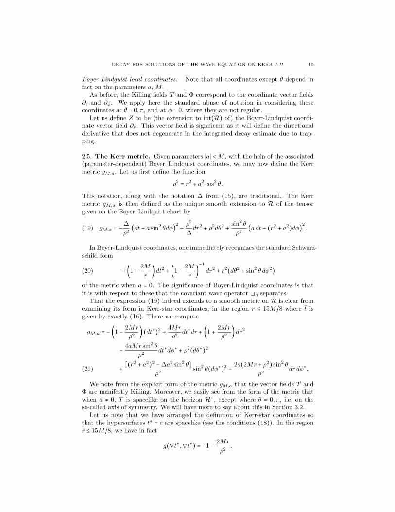
2.5. The Kerr metric. Given parameters ∣a∣ <M , with the help of the associated(parameter-dependent) Boyer–Lindquist coordinates, we may now define the Kerrmetric gM.a. Let us first define the function

ρ2= r2

+ a2 cos2 θ.

This notation, along with the notation ∆ from (15), are traditional. The Kerrmetric gM,a is then defined as the unique smooth extension to R of the tensorgiven on the Boyer–Lindquist chart by

gM,a = −∆

ρ2(dt − a sin2 θdφ)

2+ρ2

∆dr2

+ ρ2dθ2+

sin2 θ

ρ2(adt − (r2

+ a2)dφ)

2.(19)

In Boyer-Lindquist coordinates, one immediately recognizes the standard Schwarz-schild form

(20) − (1 −2M

r)dt2 + (1 −

2M

r)

−1

dr2+ r2

(dθ2+ sin2 θ dφ2

)

of the metric when a = 0. The significance of Boyer-Lindquist coordinates is thatit is with respect to these that the covariant wave operator 2g separates.

That the expression (19) indeed extends to a smooth metric on R is clear fromexamining its form in Kerr-star coordinates, in the region r ≤ 15M/8 where t isgiven by exactly (16). There we compute

gM,a = − (1 −2Mr

ρ2) (dt∗)2

+4Mr

ρ2dt∗dr + (1 +

2Mr

ρ2)dr2

−4aMr sin2 θ

ρ2dt∗dφ∗ + ρ2

(dθ∗)2

+[(r2 + a2)2 −∆a2 sin2 θ]

ρ2sin2 θ(dφ∗)2

−2a(2Mr + ρ2) sin2 θ

ρ2dr dφ∗.(21)

We note from the explicit form of the metric gM,a that the vector fields T andΦ are manifestly Killing. Moreover, we easily see from the form of the metric thatwhen a ≠ 0, T is spacelike on the horizon H+, except where θ = 0, π, i.e. on theso-called axis of symmetry. We will have more to say about this in Section 3.2.

Let us note that we have arranged the definition of Kerr-star coordinates sothat the hypersurfaces t∗ = c are spacelike (see the conditions (18)). In the regionr ≤ 15M/8, we have in fact

g(∇t∗,∇t∗) = −1 −2Mr

ρ2.


A final remark: It would be possible to define the Kerr family on the fixed R sothat one has smooth dependence up to and including the extremal case a =M , butone would have to set things up slightly differently.

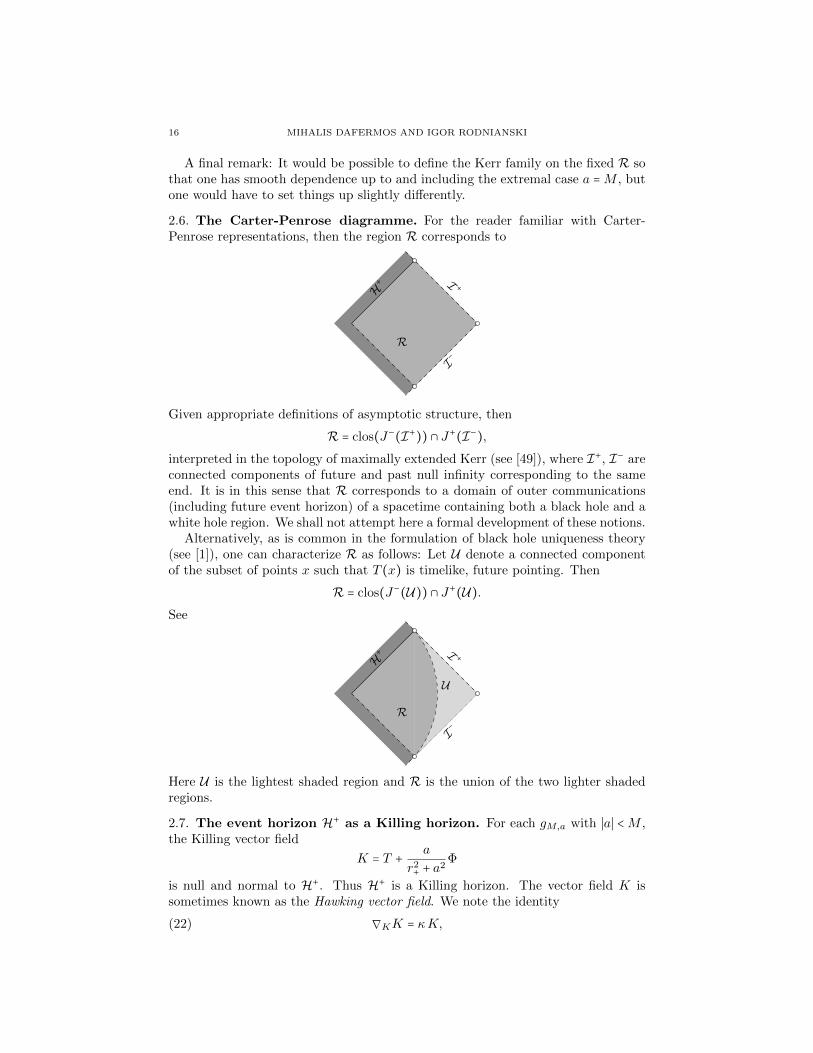
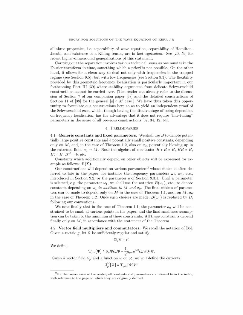
2.6. The Carter-Penrose diagramme. For the reader familiar with Carter-Penrose representations, then the region R corresponds to

H+ I +

I−R

Given appropriate definitions of asymptotic structure, then

R = clos(J−(I+)) ∩ J+(I−),

interpreted in the topology of maximally extended Kerr (see [49]), where I+, I− areconnected components of future and past null infinity corresponding to the sameend. It is in this sense that R corresponds to a domain of outer communications(including future event horizon) of a spacetime containing both a black hole and awhite hole region. We shall not attempt here a formal development of these notions.

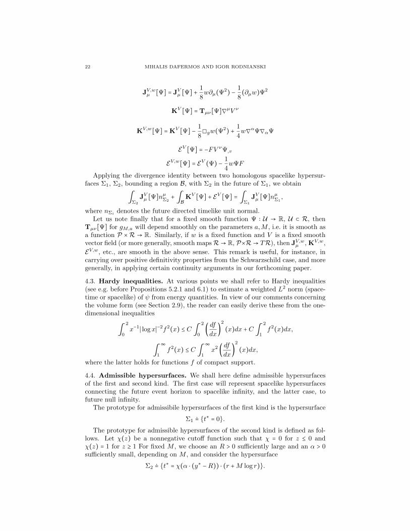
Alternatively, as is common in the formulation of black hole uniqueness theory(see [1]), one can characterize R as follows: Let U denote a connected componentof the subset of points x such that T (x) is timelike, future pointing. Then

R = clos(J−(U)) ∩ J+(U).

See

H+ I +

I−R

U

Here U is the lightest shaded region and R is the union of the two lighter shadedregions.

2.7. The event horizon H+ as a Killing horizon. For each gM,a with ∣a∣ <M ,the Killing vector field

K = T +a

r2+ + a2

Φ

is null and normal to H+. Thus H+ is a Killing horizon. The vector field K issometimes known as the Hawking vector field. We note the identity

(22) ∇KK = κK,


where

(23) κ =r+ − r−

2(r2+ + a2)

> 0.

The quantity κ is known as the surface gravity. We note that κ vanishes in theextremal case ∣a∣ =M .

We remark finally that the vector K restricted to the horizon coincides with thesmooth extension of the coordinate vector field ∂r∗ of the (r∗, t, θ, φ) coordinatesystem.

2.8. Asymptotics and angular momentum operators. Besides the smoothdependence of gM,a on a, it will be useful to remark that for fixed a and large rvalues, gM,a is very close to gM .

We may define a standard basis Ω1, Ω2, Ω3 of angular momentum operatorscorresponding to gM , such that moreover, Ω1 = Φ say. These are just a standardset of generators for the Lie algebra so(3) corresponding to the spherical symmetryof gM .

We note that Ωi span the tangent space to the S2 factors of the differential-topological product (13).

For future reference, let us introduce here the notation g/, ∇/ to denote the inducedmetric and covariant derivative from ga,M on the S2 factors of R in the differential-topological product (13).

2.9. The volume form. We shall often go back and forth between divergenceidentities which arise geometrically and those which are computed explicitly invarious coordinates. For this the following remarks may be useful.

We note that the volume form in Boyer-Lindquist coordinates satisfies

dV = v(r, θ)dt dr dVg/ with v ∼ 1

using the alternative r∗ coordinate,

dV = v(r∗, θ)dt dr∗ dVg/ with v ∼ ∆/r2

and in Kerr-star coordinates

dV = v(r, θ∗)dt∗ dr dVg/ with v ∼ 1.

Let γ denote the standard unit metric on the sphere in (θ, φ) coordinates. Wehave that g/ ∼ r2γ, and thus we may replace dVg/ in the above using

dVg/ = v(r, θ) r2 sin θ dθ dφ with v ∼ 1.

3. The geometry of Kerr

The geometry of the Kerr solution has been treated at length in the literature, seefor instance [72]. We will discuss here only those features that will be particularlyrelevant to the considerations of this paper.


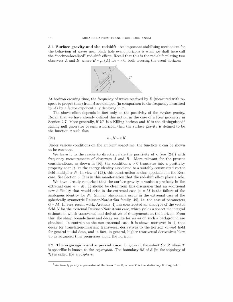
3.1. Surface gravity and the redshift. An important stabilising mechanism forthe behaviour of waves near black hole event horizons is what we shall here callthe “horizon-localised” red-shift effect. Recall that this is the red-shift relating twoobservers A and B, where B = ϕτ(A) for τ > 0, both crossing the event horizon:

H+

I+

A

B

At horizon crossing time, the frequency of waves received by B (measured with re-spect to proper time) from A are damped (in comparison to the frequency measuredby A) by a factor exponentially decaying in τ .

The above effect depends in fact only on the positivity of the surface gravity.Recall that we have already defined this notion in the case of a Kerr geometry inSection 2.7. More generally, if H+ is a Killing horizon and K is the distinguished1

Killing null generator of such a horizon, then the surface gravity is defined to bethe function κ such that

(24) ∇KK = κK.

Under various conditions on the ambient spacetime, the function κ can be shownto be constant.

We leave it to the reader to directly relate the positivity of κ (see (24)) withfrequency measurements of observers A and B. More relevant for the presentconsiderations, as shown in [36], the condition κ > 0 translates into a positivityproperty near H+ in the energy identity associated to a suitably constructed vectorfield multiplier N . In view of (23), this construction is thus applicable in the Kerrcase. See Section 5. It is in this manifestation that the red-shift effect plays a role.

We have already remarked that the surface gravity κ vanishes precisely in theextremal case ∣a∣ = M . It should be clear from this discussion that an additionalnew difficulty that would arise in the extremal case ∣a∣ = M is the failure of theanalogous identity for N . Similar phenomena occur in the extremal case of thespherically symmetric Reissner-Nordstrom family [49], i.e. the case of parametersQ =M . In very recent work, Aretakis [4] has constructed an analogue of the vectorfield N for the extremal Reissner-Nordstrom case, which yields a spacetime integralestimate in which transversal null derivatives of ψ degenerate at the horizon. Fromthis, the sharp boundedness and decay results for waves on such a background areobtained. In contrast to the non-extremal case, it is shown moreover in [4] thatdecay for translation-invariant transversal derivatives to the horizon cannot holdfor general initial data, and in fact, in general, higher transversal derivatives blowup as advanced time progresses along the horizon.

3.2. The ergoregion and superradiance. In general, the subset E ⊂R where Tis spacelike is known as the ergoregion. The boundary ∂E of E (in the topology ofR) is called the ergosphere.

1We take typically a generator of the form T + cΦ, where T is the stationary Killing field.


Under these conventions, we see easily that in the Schwarzschild case a = 0,E = ∅. If a ≠ 0, then E ≠ ∅, and ∂E ∩H+ = θ∗ = 0, π ∩H+ under our standardabuse of notation.

For all 0 < ∣a∣ <M , we havesupEr = 2M,

and thus

(25) lima→0

supEr − r+ = lim

a→0(2M − r+) = 0.

It follows that, for small ∣a∣ ≪M , the ergoregion lies very close to the horizon, inparticular, it is contained in the region where the red-shift mechanism operates, inthe sense of Section 5. More on this below.

The ergosphere allows for a particle “process”, originally discovered by Pen-rose [73], for extracting energy out of a black hole. This came to be known asthe Penrose process. In his thesis, Christodoulou [22] discovered the existence ofa quantity–the so-called irreducible mass of the black hole–which he showed to bealways nondecreasing in a Penrose process. The analogy between this quantity andentropy developed into a collection of ideas known as “black hole thermodynam-ics” [9]. This remains the subject of intense investigation from the point of view ofhigh energy physics.

In the context of solutions ψ of the wave equation, if p ∈ E , then it is no longerthe case that the energy density JTµ [ψ]n

µ(p) (see the notation of Section 4.2) isnecessarily non-negative for nµ a future-directed timelike vector at p. Thus, theconservation law for JTµ [ψ] no longer yields a priori control of a non-negative definitequantity in the derivatives of ψ. The flux of energy to null infinity can thus be largerthan the initial energy. This is the phenomenon of superradiance, first discussedby Zeldovich [89]. Moreover, a priori, this flux can be infinite. (Bounds for thestrength of superradiance were first derived heuristically by Starobinsky [80] invarious asymptotic regimes.) As discussed in the introduction, it is for this reasonthat the problem of obtaining any sort of boundedness property, even away fromthe horizon, is so difficult in Kerr. This was the difficulty which was first overcomein [35].

As in [35], the present paper exploits the fact that the “strength” of superradi-ance can be treated as a small parameter. Essentially this means that given thevector field N referred to in the section above, and given an arbitrary e > 0, thenfor sufficiently small a0 > 0, the vector field T + eN is timelike with respect to allgM,a with ∣a∣ ≤ a0. This is of course related to (25). See Section 5.3.

Let us note that in the case of arbitrary a0 <M , ∣a∣ ≤ a0, superradiance is absentif ψ is assumed axisymmetric, i.e. Φ(ψ) = 0. This is because, although T fails to beeverywhere causal, the flux JTµ [ψ]n

µH+ through the horizon is nonnegative. This in

turn is related to the fact that the null generator nH+ of the horizon is of the formT + c(a,M)Φ.

In the general case of arbitrary a0 <M , ∣a∣ ≤ a0, without axisymmetry, the effectof superradiance cannot be treated as a small parameter and is now a priori stronglycoupled to the other difficulties. In particular, there are trapped null geodesics (seeSection 3.3) that remain in the ergoregion for all positive affine time. Nonetheless,it turns out that the situation is much better than it initially appears and thedifficulty of superradiance can again be resolved, combining the ideas of [32] withthose of the present paper. See further comments in Section 5.3 and our companion


paper [38], where the necessary constructions of our forthcoming Part III [39] aregiven in detail.

3.3. Separability of geodesic flow and trapped null geodesics. The highfrequency behaviour of solutions to wave equations is intimately related to theproperties of geodesic flow.

In the Schwarzschild case a = 0, geodesic flow is easily understood because theHamilton-Jacobi equations separate. This in turn follows immediately from thedimensionality of the span of the Killing fields T,Ω1,Ω2,Ω3. Geodesic flow on theSchwarzschild metric is described in detail in many textbooks. One sees from theresulting equations that there are null geodesics which for all affine time remain onthe hypersurface r = 3M , the so-called photon sphere. With reference to suitableasymptotic notions, we can make the following more general statement: If γ(s) isa future-directed inextendible null geodesic in Schwarzschild (R, gM,0) with γ(s) ∈R ∖H+ for all s > s0, such that moreover for all p ∈ I+, ∃s such that γ(s) /∈ J−(p),then lims→∞ r(γ(s)) = 3M .

As already mentioned in the introduction, in view of general results due toRalston [76], the above property restricts the type of decay statement that one canhope to prove. The constructions of the energy currents of [14, 32, 34, 12] andsubsequent papers, used to prove integrated decay, are thus intimately related totrapped null geodesics, in particular, the vector field multiplier X related to thecurrents JX,w applied there, vanishes precisely at r = 3M .

Turning now to the general Kerr case, remarkably, as discovered by Carter [17],geodesic flow admits, besides the conserved quantities associated to the Killingfields T and Φ, a third non-trivial conserved quantity (the ‘Carter constant’). Thus,geodesic flow remains separable and can be completely understood. The dynamicsis described in some detail in [19].

In contrast to the Schwarzschild case, there are now null geodesics with constantr for an open range of Boyer-Lindquist-r values. However, restricting to geodesicssharing a fixed triple of the nontrivial conserved quantities, there is at most oner-value, depending on the triple, to which all null geodesics neither crossing H+,nor approaching I+, must necessarily asymptote to towards the future.

The above suggests that the underlying dynamics of geodesic flow is similar(for the entire range ∣a∣ < M) to the Schwarzschild case, but to capture this inthe high frequency regime, the proper generalisation of the currents JX must befrequency-localised so as to vanish at an r-value depending on quantised versionsof the conserved quantities corresponding to trapped null geodesics.

There is a convenient way of doing phase space analysis in Kerr spacetimes whichis strongly linked to their geometry and the dynamics of geodesic flow. Namely, asdiscovered again by Carter [18], the wave equation itself can be formally separated,and the separation introduces frequencies ω, m, and λm`. which can be indeedthought of as quantised versions of the conserved quantities associated to geodesicflow.

None of these separability properties is in fact accidental! Walker and Pen-rose [86] showed shortly thereafter that both the complete integrability of geodesicflow and the formal separability of the wave equation have their fundamental originin the presence of a Killing tensor. It turns out that, in view of Ricci flatness,


all three properties, i.e. separability of wave equation, separability of Hamilton-Jacobi, and existence of a Killing tensor, are in fact equivalent. See [20, 59] forrecent higher-dimensional generalisations of this statement.

Carrying out the separation involves various technical issues as one must take theFourier transform in time, something which a priori is not possible. On the otherhand, it allows for a clean way to deal not only with frequencies in the trappedregime (see Section 9.5), but with low frequencies (see Section 9.3). The flexibilityprovided by this geometric frequency localisation is particularly important in ourforthcoming Part III [39] where stability arguments from delicate Schwarzschildconstructions cannot be carried over. (The reader can already refer to the discus-sion of Section 7 of our companion paper [38] and the detailed constructions ofSection 11 of [38] for the general ∣a∣ < M case.) We have thus taken this oppor-tunity to formulate our constructions here so as to yield an independent proof ofthe Schwarzschild case, which, though having the disadvantage of being dependenton frequency localisation, has the advantage that it does not require “fine-tuning”parameters in the sense of all previous constructions [32, 34, 12, 64].

4. Preliminaries

4.1. Generic constants and fixed parameters. We shall use B to denote poten-tially large positive constants and b potentially small positive constants, dependingonly on M , and, in the case of Theorem 1.2, also on a0, potentially blowing up inthe extremal limit a0 → M . Note the algebra of constants: B + B = B, BB = B,Bb = B, B−1 = b, etc.

Constants which additionally depend on other objects will be expressed for ex-ample as follows: B(Σ).

Our constructions will depend on various parameters2 whose choice is often de-ferred to late in the paper, for instance the frequency parameters ω1, ω3, etc.,introduced in Section 9.2, or the parameter q of Section 9.3.1. Until a parameteris selected, e.g. the parameter ω1, we shall use the notation B(ω1), etc., to denoteconstants depending on ω1 in addition to M and a0. The final choices of parame-ters can be made to depend only on M in the case of Theorem 1.1, and, on M , a0

in the case of Theorem 1.2. Once such choices are made, B(ω1) is replaced by B,following our conventions.

We note finally that in the case of Theorem 1.1, the parameter a0 will be con-strained to be small at various points in the paper, and the final smallness assump-tion can be taken to the minimum of these constraints. All these constraints dependfinally only on M , in accordance with the statement of the Theorem.

4.2. Vector field multipliers and commutators. We recall the notation of [35].Given a metric g, let Ψ be sufficiently regular and satisfy

2gΨ = F.

We define

Tµν[Ψ] ≐ ∂µΨ∂νΨ −1

2gµνg

αβ∂αΨ∂βΨ.

Given a vector field Vµ and a function w on R, we will define the currents

JVµ [Ψ] = Tµν[Ψ]V ν

2For the convenience of the reader, all constants and parameters are referred to in the index,with reference to the page on which they are originally defined.


JV,wµ [Ψ] = JVµ [Ψ] +1

8w∂µ(Ψ

2) −

1

8(∂µw)Ψ2

KV[Ψ] = Tµν[Ψ]∇

µV ν

KV,w[Ψ] = KV

[Ψ] −1

82gw(Ψ2

) +1

4w∇αΨ∇αΨ

EV[Ψ] = −FV νΨ,v

EV,w

[Ψ] = EV(Ψ) −

1

4wΨF

Applying the divergence identity between two homologous spacelike hypersur-faces Σ1, Σ2, bounding a region B, with Σ2 in the future of Σ1, we obtain

∫Σ2

JVµ [Ψ]nµΣ2+ ∫B

KV[Ψ] + E

V[Ψ] = ∫

Σ1

JVµ [Ψ]nµΣ1,

where nΣi denotes the future directed timelike unit normal.Let us note finally that for a fixed smooth function Ψ ∶ U → R, U ⊂ R, then

Tµν[Ψ] for gM,a will depend smoothly on the parameters a,M , i.e. it is smooth asa function P ×R → R. Similarly, if w is a fixed function and V is a fixed smoothvector field (or more generally, smooth mapsR→ R, P×R→ TR), then JV,wµ , KV,w,

EV,w, etc., are smooth in the above sense. This remark is useful, for instance, incarrying over positive definitivity properties from the Schwarzschild case, and moregenerally, in applying certain continuity arguments in our forthcoming paper.

4.3. Hardy inequalities. At various points we shall refer to Hardy inequalities(see e.g. before Propositions 5.2.1 and 6.1) to estimate a weighted L2 norm (space-time or spacelike) of ψ from energy quantities. In view of our comments concerningthe volume form (see Section 2.9), the reader can easily derive these from the one-dimensional inequalities

∫

2

0x−1

∣ logx∣−2f2(x) ≤ C ∫

2

0(df

dx)

2

(x)dx +C ∫2

1f2

(x)dx,

∫

∞

1f2

(x) ≤ C ∫∞

1x2

(df

dx)

2

(x)dx,

where the latter holds for functions f of compact support.

4.4. Admissible hypersurfaces. We shall here define admissible hypersurfacesof the first and second kind. The first case will represent spacelike hypersurfacesconnecting the future event horizon to spacelike infinity, and the latter case, tofuture null infinity.

The prototype for admissibile hypersurfaces of the first kind is the hypersurface

Σ1 ≐ t∗ = 0.

The prototype for admissible hypersurfaces of the second kind is defined as fol-lows. Let χ(z) be a nonnegative cutoff function such that χ = 0 for z ≤ 0 andχ(z) = 1 for z ≥ 1 For fixed M , we choose an R > 0 sufficiently large and an α > 0sufficiently small, depending on M , and consider the hypersurface

Σ2 ≐ t∗ = χ(α ⋅ (y∗ −R)) ⋅ (r +M log r).


Note that Σ1 and (for suitable choice3 of R, α) Σ2 are spacelike for all gM,a

where 0 ≤ a0 < M , ∣a∣ ≤ a0. Notice also that for all choices of a, the hypersurfaceΣ2 asymptotes to null infinity with respect to usual constructions of asymptoticstructure. For reasons concerning dependence of constants on a0 in the statementsof our theorems, it is convenient to require these properties for all hypersurfaces tobe considered. This will thus be encorporated into the definition below:

Definition 4.1. Let 0 ≤ a0 < M . We will call a hypersurface-with-boundary Σadmissible of the first kind with respect to a0, M , if the following hold:

(1) Σ is spacelike with respect to gM,a for all ∣a∣ ≤ a0.(2) Σ ⊂R is closed as a subset, and ∂Σ ⊂H+ is compact and thus a topological

sphere.(3) There exists a τ ∈ (−∞,∞) such that for all ε > 0, there exists an y∗ε > 0

such that

Σ ∩ y∗ ≥ y∗ε ⊂ ⋃∣τ ′∣≤ε

ϕτ+τ ′(Σ1)

We call Σ admissible of the second kind with respect to a0, M , if the above holdwhere Σ1 is replaced by Σ2.

We will say that Σ is admissible . . . with respect to M if the there exists an a0 > 0sufficiently small such that the above is true.

Note that for an admissible Σ, its future domain of dependence with respect toall gM,a is given by

D+(Σ) = ⋃

τ∈[0,∞)ϕτ(Σ)

The main theorem of the present paper do not in fact distinguish between the typeof admissible hypersurfaces. These definitions are useful more to keep track of thedependence of constants. In the theorem of [40], stated here as Theorem 1.4, it isessential to consider admissible hypersurfaces of the second kind.

4.5. Well-posedness. First let us quote a general well-posedness statement.

Proposition 4.5.1. Let s ≥ 1, M > a0 ≥ 0 be fixed, and let Σ be an arbitraryadmissible hypersurface (of either kind) in R. Let ψ ∈ Hs

loc(Σ), ψ′ ∈ Hs−1loc (Σ).

Then for all ∣a∣ ≤ a0, there exists a unique solution ψ of 2gψ = 0 with g = gM,a inD+(Σ) such that

ψ ∈ C0τ∈[0,∞)(H

sloc(ϕτ(Σ))) ∩C1

τ∈[0∞)(Hs−1loc (ϕτ(Σ)))

and ψ∣Σ = ψ, (nΣψ)∣Σ = ψ′. Moreover, if X ⊂ Σ is open and ψ ∈ Hsloc(Σ), ψ′ ∈

Hs−1loc (Σ) such that ψ = ψ and ψ′ = ψ′ in X, then the corresponding unique solutions

ψ, ψ satsify ψ = ψ in D+(X).Finally the map (ψ,ψ′) × a ↦ ψa, where ψa denotes ψ above with g = gM,a is

C0 ×C∞.

The above theorem implies that solutions of the wave equation arising fromappropriate initial data exist globally, and their regularity in L2-based Sobolevspaces is preserved on any Cauchy surface, and moreover, the solutions dependcontinuously on initial data and smoothly on the parameters.

3Let these choices be made once and for all.


4.6. A reduction. First let us note that by extending initial data, an easy domainof dependence argument, and the fact that T is timelike for all Kerr metrics nearinfinity, one can show the following:

Proposition 4.6.1. Fix M > ∣a0∣ ≥ 0. Let Σ be admissible with respect to M , a0, ofthe first or second kind. Then there exists a constant B = B(Σ,M) = B(ϕτ(Σ),M)

such that the following holds:Let ψ be a solution of the wave equation (2) for g = gM,a on D+(Σ), with ∣a∣ ≤ a0,

such that ψ, nΣψ are smooth and compactly supported on Σ. Then there exists aτ ′ and a smooth solution ψ of (2) on R such that D+(Σ) ⊂ t∗ ≥ τ ′,

ψ = ψ

in D+(Σ), ψ, ∂∗t ψ are of compact support on t∗ = τ ′ and

B−1∫

ΣJNµ [ψ]nµΣ ≤ ∫

t∗=τ ′JNµ [ψ]nµt∗=τ ′ ≤ B ∫

ΣJNµ [ψ]nµΣ,

where N is the vector field of Section 5.

Taking the difference ψ − ψ∞, it follows easily from Proposition 4.6.1, a Hardyinequality and a density argument that without loss of generality, we may assumein Theorems 1.1, 1.2 that Σ = t∗ = 0 and ψ is smooth and of compact support.We shall assume this reduction starting in Section 8.

4.7. Uniform boundedness. Let us note that the results of [35] and the aboveproposition yield in particular

Theorem 4.1. Fix M > 0. Let Σ be admissible with respect to M . Then thereexists a constant B = B(Σ,M) = B(ϕτ(Σ),M) and a positive constant ε = ε(M),such that for all ∣a∣ ≤ ε, if ψ be a sufficiently regular solution of (2) on D+(Σ) withg = gM,a, then

∫ϕτ (Σ)

JNµ [ψ]nµϕτ (Σ) ≤ B ∫

ΣJNµ [ψ]nµΣ,

∫H+∩D+(Σ)JnH+µ [ψ]nµH+ ≤ B ∫

ΣJNµ [ψ]nµΣ,

where N is the vector field of Section 5. The same statement holds with arbitrary∣a∣ ≤ a0 <M if Σ is assumed admissible with respect to M , a0, for ψ with Φψ = 0.

We referred to N of Section 5 simply to fix the vector field once and for all. Ifone does not wish to refer to that particular vector field, one can alternatively takean arbitrary ϕτ -invariant timelike vector field N such that N = T for sufficientlylarge r. The constant B will then depend also on the choice of that N .

We shall avoid appealing to Theorem 4.1 in the case of the proof ofTheorem 1.1, in order to have a self-contained proof. See the discussionof Section 5.3.

In the case of Theorem 1.2, the proof of Theorem 4.1 should be considered asmore elementary than the considerations of the present paper in view precisely ofthe absense of superradiance, so, in particular, we shall freely use it.

This distinction between the proofs of Theorem 1.1 and 1.2 foreshadows theprinciple (essential in our forthcoming Part III [39]) that the superradiant andnonsuperradiant modes must be treated separately in the general ∣a∣ <M case. Seethe discussion in Section 7.3 of our companion [38].


5. A JN multiplier current and the red-shift

In this section, we define a timelike vector field N whose multiplier currentJN captures the red-shift effect. The existence of this current is in fact a generalproperty of stationary black hole spacetimes with Killing horizons of positive surfacegravity. We shall discuss in Section 5.3 how the properties of this current can beused to overcome the difficulty of superradiance in the small a0 case. We shall thenrecall in Section 5.4 the good commutation properties of the wave operator 2g witha related vector field Y (used in the construction of N) on H+, properties whichagain arise from the positivity of the surface gravity. Finally, in Section 5.5, weshall apply commutations with T and Y to infer Theorem 1.3 from Theorems 1.1and 1.2.

5.1. The construction of N . First, the completely general statement specialisedto a given Kerr metric: Theorem 7.1 of [36] yields

Proposition 5.1.1. Let ∣a∣ < M , ga,M be the Kerr metric and R, etc., be asbefore. There exist positive constants b = b(a,M) and B = B(a,M), parametersr1(a,M) > r0(a,M) > r+, and a ϕτ -invariant timelike vector field N = N(a,M) onR such that

(1) KN [Ψ] ≥ bJNµ [Ψ]Nµ for r ≤ r0

(2) −KN [Ψ] ≤ B JNµ [Ψ]Nµ, for r ≥ r0

(3) T = N for r ≥ r1,

where the currents are defined with respect to gM,a.

Proof. We recall the proof briefly: Given a Kerr metric g = gM,a and a constantσ > 0, we first note that we may define a vector field Y such that on H+ we have:

(a) Y is future directed null with g(Y,K) = −2,(b) ∇Y Y = −σ(Y +K) and(c) LTY = LΦY = 0,

where K is the Hawking vector field of Section 2.7.4 If we choose σ sufficientlylarge and r0(a,M) sufficiently close to r+, then, defining

N =K + Y, in r ≤ r0(a,M),

then, using (23), one sees easily that requirement 1 will hold, and moreover N istimelike in this region. The choice of Y , r0(a,M) can clearly be made to smoothlydepend on a. If r1(a,M) > r0(a,M) is such that T is timelike for r ≥ r1(a,M) itsuffices to smoothly extend N as a timelike vector field invariant to the Lie flow ofΦ and T such that N = T in r ≥ r1(a,M), satisfying requirement 3. Requirement 2then follows by compactness.

Moreover, in view of (25) we clearly have the following

Proposition 5.1.2. Fix M > 0. Then a ϕτ -invariant timelike vector field N canbe defined on the manifold R such that for a0 sufficiently small, and ∣a∣ ≤ a0 <M ,then 1, 2 and 3 of Proposition 5.1.1 hold where then b and B, r1, r0 can be chosento depend only on M with r1 ≤ 5M/2, and 2. can be strengthened to the statement

−KN[ψ] ≤ B JTν [Ψ]T ν , T is timelike for r ≥ r0.

4In Theorem 7.1 of [36] we in fact constructed Y to be only invariant under the flow definedby K, but in the presence of our two Killing fields T and Φ, one can clearly arrange also for this.


Let us note that in the case of ∣a∣ ≪ M , both the above propositions followdirectly from the existence of a vector field N on Schwarzschild satisfying the abovestatements and smooth dependence of the Kerr family on a (see Section 4.2), asfirst observed and exploited in [32]. See also [33, 34, 35]. In this case then, we needthus not appeal to the more general construction of [36].

In what follows, in the setting of Theorem 1.1, we shall always assume a0 suffi-ciently small so that Proposition 5.1.2 applies. Thus, in the setting of Theorem 1.1,we have in particular that T is timelike for r ≥ r0. In the setting of Theorem 1.2,all we know is that T is timelike for r ≥ r1.

5.2. The red-shift estimate. Given arbitrary r satisfying r+ < r ≤ r0 and δ > 0,then applying the energy identity of JχN in D+(Σ) ∩ J−(ϕτ(Σ)), where χ(r) is a

cutoff function with χ = 1 for r ≤ r and χ = 0 for r ≥ r + δ, and a Hardy inequalitywe obtain the following

Proposition 5.2.1. Let g = gM,a for ∣a∣ ≤ a0 < M , and let r0 be as in the abovePropositions. Then the following is true. Let Σ be an admissible hypersurface forM,a0. For all r+ ≤ r ≤ r0 and δ > 0, there exists a positive constant B = B(Σ, r, δ) =

B(ϕτ(Σ), r, δ), such that for all solutions ψ of (2) on D+(Σ) with g = gM,a, then

∫D+(Σ)∩J−(ϕτ (Σ))∩r≤r

(JNµ [ψ]Nµ+ ∣ log(∣r − r+∣)

−2∣∣r − r+∣

−1ψ2)

+∫H+∩D(Σ)∩J−(ϕτ (Σ))JNµ [ψ]nµH+ + ∫

ϕτ (Σ)∩r≤rJNµ [ψ]nµ

≤ B ∫Σ

JNµ [ψ]nµ +B ∫D+(Σ)∩J−(ϕτ (Σ))∩r≤r≤r+δ

(JNµ [ψ]Nµ+ ψ2

)

Recall that the additional dependence of B onM and a0 is now implicit accordingto our conventions.

5.3. The red-shift vs. superradiance. Superradiance concerns the fact that T isnot everwhere timelike. The smallness of superradiance with respect to the redshiftin the setting of Theorem 1.1 can be quantified by the following

Proposition 5.3.1. There exists an a0 > 0 and a differentiable nonnegative func-tion e0(a) defined for ∣a∣ ≤ a0, such that e0(0) = 0, a ⋅ (e0)

′(a) ≥ 0, and such thatT + eN is timelike for e > e0 in r > r+, and such that for all τ ′ ≥ τ , the followinginequalities hold:

∫Στ ′

JT+eNµ [ψ]Nµ≤ ∫

ΣτJT+eNµ [ψ]Nµ

+Be∫D+(Στ )∩J−(ϕτ ′(Σ))∩r≤r≤r+δ

JNµ [ψ]Nµ

∫H+∩τ≤t∗≤τ ′JT+eNµ [ψ]nµH+ ≤∫

ΣτJT+eNµ [ψ]Nµ

+Be∫D+(Στ )∩J−(ϕτ ′(Σ))∩r≤r≤r+δ

JNµ [ψ]Nµ,

with B = B(Σ, r, δ), r+ < r ≤ r0, δ > 0, as in the previous proposition.

Proof. The existence of an e0(a) as described so that T + eN is timelike is clear.Now just add e times the previous proposition to the energy identity of JT , for ane such that T + eN is timelike, and use that T is Killing, i.e. KT = 0, and that T istimelike for r ≥ r0, and thus JT+eNµ [ψ]Nµ ∼ JTµ [ψ]N

µ on r ≥ r0.


The above proposition is of course implied by Theorem 4.1 of [35] but we includeit as an independent statement so as to circumvent appeal to this theorem in thecase of the proof of Theorem 1.1. For this, we shall also need the following

Proposition 5.3.2. Given arbitrary ε > 0, there exists an a0 > 0 depending on ε,such that for ∣a∣ ≤ a0, and 1 ≥ e ≥ e0(a),

(26) ∫ϕτ (Σ)

JT+eNµ [ψ]Nµ≤ (1 +Be)∫

ΣJT+eNµ [ψ]Nµ, ∀0 ≤ τ ≤ ε−1,

(27) ∫D+(Σ)∩J−(ϕε−1(Σ))∩r0≤r≤r1

JNµ [ψ]Nµ≤ B ∫

ΣJNµ [ψ]Nµ.

Proof. The first inequality follows immediately from the second. The second in-equality follows from the fact that (27) holds for the Schwarzschild metric gM for allε (note the restriction on r1 in Proposition 5.1.2 which guarantees that the domainof integration on the left hand side is separated from the Schwarzschild photonsphere) together with the stability considerations of Section 4.2.

We note that the necessary Schwarzschild result was proven in [32]. The currentpaper can be read independently of [32], as follows: While the present propositionis appealed to in the proof of Theorem 1.1, if the latter is specialised to the casea0 = 0, then, just as in the m = 0 case, the use of the present proposition is in factnot necessary, as appeal has only been made to circumvent use of Theorem 4.1 inthe case a ≠ 0. Thus, the proof of Theorem 1.1 specialised to a0 = 0 yields thepresent proposition, which can then be used in the proof of Theorem 1.1 for thegeneral ∣a∣ ≪M case.

The significance of the above two propositions is the following: As in the proofof Theorem 4.1 of [35], we shall be able to absorb the boundary terms of our virialidentities for sufficiently small a using solely Propositions 5.3.1 and 5.3.2 exploitingthe fact that one can take e very close to 0. It is the use of this argument thatmathematically represents one of the insights first used in [35], namely:

If superradiance is sufficiently weak, it can be overcome provided one canconstruct a virial current with positive definite divergence, whose boundaryterms can be controlled with the positive definite current formed by addinga small amount of the red-shift current JN to the conserved energy currentJT .

What we are essentially able to avoid using here is the second main insight of [35],summarised as follows:

To obtain just the boundedness statement, it suffices to construct a virialcurrent as above for the projection of the solution to its superradiant fre-quencies. Such a projection can be defined for arbitrary axisymmetric sta-tionary black hole spacetimes whose Killing fields span the null generatorof the horizon. Moreover, for suitably small such perturbations of Schwarz-schild, this projection is not “trapped”, thus the existence of the virial cur-rent follows from stability considerations from Schwarzschild!

The above insight allowed boundedness to be understood without understandingdecay and without understanding trapping. This is why the result of [35] is sogeneral, not requiring the properties of geodesic flow which are so crucial for thepresent paper. We have no need for the second insight here, precisely because, for


the special case of the Kerr solution, we are indeed proving decay, that it is to say,we are indeed producing such a virial current for the total solution.

It is to highlight this distinction that we have been careful to avoid use of ourgeneral boundedness theorem [35] and its superradiant projection. The reader hop-ing that one can understand the Kerr family without understanding superradiancewill be severely disappointed however! In particular, the superradiant projectionof [35] is used heavily in our forthcoming [39] which considers the general case∣a∣ <M , precisely because superradiance can no longer be treated simply as a smallparameter and the above insight is not sufficient. See the discussion in Section 7.3of our companion paper [38], and Section 11 of [38] for the details of the necessaryconstructions in all frequency ranges for the general case.

5.4. Red-shift commutation. We specialise Theorem 7.2 of [36] to the Kerr case.

Proposition 5.4.1. Let g = gM,a and Y be as in Proposition 5.1.1. Then, on H+,extending K to a translation invariant standard null frame E1,E2,K,Y , then forall k ≥ 0 and multi-indices m = (m1,m2,m3.m4),

2g(YkΨ) = κkY

k+1Ψ + ∑∣m∣≤k+1,m4≤k

cmEm1

1 Em2

2 Lm3Y m4Ψ

where κk > 0.

The above proposition, which is another manifestation of the red-shift effect,effectively allows us not only to apply a transversal vectorfield to the horizon asa multiplier, but also as a commutator. This is fundamental for retrieving higherorder statements as in Theorem 1.3.

5.5. The higher order statement. Commuting the wave equation with T and Y ,in the latter case applying Propostion 5.4.1, we show the statement of Theorem 1.3,given Theorems 1.1 and 1.2.

For j = 1: We commute the equation first with T . It follows that the estimates ofTheorem 1.1 or 1.2 hold with Tψ in place of ψ. Now we commute also with Y andfollow [35, 36]. The quantity Y ψ satisfies a wave equation with an inhomogeneousterm, but by Proposition 5.4.1, the most dangerous term arising in EN [Y ψ] (recallthe notation of Section 4.2) has a good sign sufficiently near the horizon. In thecase of the assumptions of Theorem 1.1, we may assume that T is strictly timelikeoutside this region. Elliptic estimates then suffice to bound all remaining termsin EN [Y ψ] from the good terms in KN [Y ψ] and those already bounded by thecommutation by T . In the case of m = 0, T is effectively timelike everywhereexcept the horizon from the perspective of axisymmetric solutions, in the sensethat for every x ∈R ∩H+ there is a T + c(x)Φ which is timelike in a neighborhoodof x. Thus, again, all terms not manifestly controlled can be easily obtained byelliptic estimates in view of the fact that NNψ is controlled locally in L2.

The case of higher j is similar and the required positivity of the most danger-ous additional terms appearing in EN [Y jψ] is precisely that provided by Proposi-tion 5.4.1 above for j = k ≥ 2.

Recall that in our forthcoming Part III [39], it will be shown that the statementof Theorem 1.2 is true without the restriction (9). The above arguments can beextended to show that, in general, given parameters M > a for which the statementof Theorem 1.2 holds without the restriction (9), one can infer the validity ofTheorem 1.3 for those parameters M , a. Let us first note that Proposition 5.4.1


still applies, yielding positivity for the most dangerous terms in EN [Y ψ] in a smallneighborhood of the horizon. The only additional difficulty is that one can no longerappeal to smallness of a0 (as in the case of Theorem 1.1) to argue that T is timelikeoutside this region and thus, outside this region, all second derivatives can becontrolled by the integrated decay bound applied to Tψ (a statement which, as wesaw above, can similarly be inferred in the case of Theorem 1.2 using the assumptionof axisymmetry). In the more general setting, in addition to commutations with Tand Y as above, we must simply also commute with χΦ (where χ = 1 for r ≤ R,and ∇χ is thus supported away from trapping), and exploit the fact that the spanof T and Φ is timelike away from the horizon. The error terms resulting in thecommutation with χΦ are easily absorbed with the integrated decay statement.Thus, commutations with Y , T and χΦ ensure that one always has a timelikedirection in the span of commutators up to and including the horizon. Applicationof elliptic estimates allows one as before to absorb all error terms and obtain allsecond derivatives. One then proceeds by induction on j. We shall insert the detailsof this more general argument with the completion of Part III [39].

6. A current for large r

We construct here a current JX,w as follows. Recall (see e.g. [35]) that in theSchwarzschild geometry gM , defining

X = f(r∗)∂r

w = 2f ′(r∗) + 41 − 2M/r

rf − 2δ

1 − 2M/r

r1+δ f,

we have

KX,wgM

[Ψ] = (f ′

1 − 2M/r−

fδ

2r1+δ )(∂r∗Ψ)2+

fδ

2r1+δ (∂tΨ)2

+f (r − 3M

r2−δ(r − 2M)

2r2+δ ) ∣∇/Ψ∣2−

1

22wΨ2

where ′ denotes differentiation with respect to r∗. Let χ be a cutoff function suchthat χ = 1 for r ≥ R, χ = 0 for r ≤ R − 1 and let δ > 0. Choose now

f = χ(1 − r−δ)∂r.

We note that for R sufficiently large, we have

KX,wgM

(Ψ) ≥ b(δ) (r−1−δ(∂rΨ)

2+ r−1−δ

(∂tΨ)2+ r−1

∣∇/Ψ∣2gM

+ r−3−δΨ2)

and that this inequality is preserved when X, w, are defined for gM,a again asabove, where ∣∇/Ψ∣2gM is now replaced by ∣∇/Ψ∣2

g/defined in the sense of Section 2.9.

From the energy identity of JX,w and a Hardy inequality to control 0’th orderterms on the boundary, we have

Proposition 6.1. Fix M > 0, let Σ be an admissible hypersurface for M , and let e0

be as above. For each δ > 0, there exist positive values R0 < R, and positive constantsB = B(δ,Σ) = B(δ,ϕτ(Σ)) such that for all Kerr metrics gM,a with ∣a∣ ≤ a0 <M , if


ψ denotes a solution of (2) with g = gM,a and ψ∞ = 0, then for all τ ≥ 0

∫D+(Σ)∩J−(ϕτ (Σ))∩r≥R

r−1(r−δ ∣∂rψ∣

2+ r−δ ∣∂tψ∣

2+ ∣∇/ψ∣2

g/+ r−2−δψ2

)

≤B ∫Σ

JT+e0Nµ [ψ]nµΣ +B ∫ϕτ (Σ)

JT+e0Nµ [ψ]nµΣ

+B ∫D+(Σ)∩J−(ϕτ (Σ))∩R0≤r≤R

(∣∂rψ∣2+ ∣∂tψ∣

2+ ∣∇/ψ∣2

g/+ ψ2

).

7. Separation

As described in Section 3.3, we will exploit Carter’s separation of the waveequation [18] to frequency-localise our virial type estimates in a manner particularlysuited to the local and global geometry of Kerr. The separation of 2gψ = 0 requirestaking the Fourier transform in t, and then expanding into what are known asoblate spheroidal harmonics. Since, a priori, we do not know that solutions ψ(t, ⋅)of our problem are L2(dt), we must in fact apply this separation to solutions of theinhomogeneous equation

(28) 2gΨ = F,

where Ψ is related to ψ by the application of a suitable cutoff. We will defer thediscussion of such cutoffs to Section 8, and will in the meantime in Section 7.2 belowgive a general discussion of solutions of (28) in r > r+ for which one can indeed takethe Fourier transform (see Section 7.2) in t. First, however, we quickly review theclassical oblate spheroidal harmonics.

7.1. Oblate spheroidal harmonics. Let L2(sin θ dθ dφ) denote the space of complex-valued L2 functions on the sphere with standard spherical coordinates θ, φ. Let L2

m

denote the eigenspace of ∂φ with eigenvalue m. Recall that

L2= ⊕m∈Z

L2m

orthogonally, and that

(29) L2m = L2

R(sin θ dθ)⊗Ceimφ.For ξ ∈ R, define the operator P (ξ) on a suitable dense subset of L2(sin θ dθ dφ)

by

P (ξ) f = −1

sin θ

∂

∂θ(sin θ

∂

∂θf) −

∂2f

∂φ2

1

sin2 θ− ξ2 cos2 θf.

Note that P (0) is the standard spherical Laplacian, whereas P (ξ) in fact corre-sponds to the Laplacian on an oblate spheroid. We have certainly that [P (ξ), ∂φ] =0 and thus P (ξ) preserves L2

m, and under the identification (29), P (ξ) induces anoperator Pm(ξ) defined on a dense subset of L2(sin θ dθ) by

Pm(ξ) f = −1

sin θ

d

dθ(sin θ

d

dθf) +

m2

sin2 θf − ξ2 cos2 θf.

The following proposition is classical and can be distilled from standard elliptictheory and the form of Pm:

Proposition 7.1.1. Let ξ ∈ R. There exists a complete basis of L2(sin θ dθ dφ) ofeigenfunctions of P (ξ) of the form Sm`(ξ, cos θ)eimφ, with real eigenvalues λm`(ξ):

P (ξ)Sm`(ξ, cos θ)eimφ = λm`(ξ)Sm`(ξ, cos θ)eimφ


where for each m ∈ Z, the collection Sm`(ξ, cos θ)eimφ are a basis in L2m of real

eigenfunctions of Pm(ξ):

Pm(ξ)Sm`(ξ, cos θ) = λm`(ξ)Sm`(ξ, cos θ)

indexed by the set ` ≥ ∣m∣. The functions Sm`(ξ, cos θ) are smooth in ξ and θ, and,λm`(ξ) is smooth in ξ. Finally, for ξ = 0, these reduce to spherical harmonics, i.e.Sm`(0, cos θ)eimφ = Ym`, where Ym` denote the standard spherical harmonics, and

λm`(0) = `(` + 1).

The functions Sm` are known classically as oblate spheroidal harmonics.Let us introduce the notation

(30) α(ξ)m` = ∫

2π

0dϕ∫

1

−1d(cos θ)α(θ, φ) e−imφSm`(ξ, cos θ).

The completeness and orthogonality conditions of Proposition 7.1.1 are givenexplicitly below:

∫

2π

0dϕ∫

1

−1d(cos θ)eimφSm`(aω, cos θ) e−im

′φSm′`′(ξ, cos θ) = δmm′δ``′ ,

(31) α(θ, φ) =∑m`

α(ξ)m`Sm`(ξ, cos θ)eimφ.

The statement (31) is to be understood in L2(sin θ dθ dφ), but, if α(θ, φ) is in fact,say, a smooth function on the standard sphere, then (31) holds pointwise in thetopology of the sphere. (We shall not require such pointwise statements, however.)

In the application to the Kerr geometry, ξ = aω for ω ∈ R, where ω will be afrequency associated to the Fourier transform with respect to t of a cutoff versionof the solution ψ. We note that the case of complex ξ is also of interest in theformal mode analysis associated to this problem (see for instance [87]). In view ofour setting, however, we shall only need to consider real ξ here.

Let us note that from the smooth dependence statement of Proposition 7.1.1(applied with the application ξ = aω in mind) one immediately obtains

Proposition 7.1.2. Given any ω1 > 0, λ1 > 0, and ε > 0, then there exists an a1 > 0such that for ∣a∣ < a1, ∣ω∣ ≤ ω1, and λm` ≤ λ1,

∣λm`(aω) − `(` + 1)∣ ≤ ε.

Rewriting the equation for the oblate spheroidal function

−1

sin θ

d

dθ(sin θ

d

dθSm`) +

m2

sin2 θSm` = λm`Sm` + a

2ω2 cos2 θSm`,

the smallest eigenvalue of the operator on the left hand side of the above equationis ∣m∣(∣m∣ + 1). This implies that

Proposition 7.1.3.

(32) λm`(aω) ≥ ∣m∣(∣m∣ + 1) − a2ω2.

The above propositions will be all that we require about λm`. For a more detailedanalysis of λm`, see [45].

Let us finally note that by integration by parts and the above orthogonality weobtain


Proposition 7.1.4.

∫ ∣γ∇α∣2γ sin θ dθ dφ − ∫ ξ2 cos2 θ ∣α∣2 sin θ dθ dφ = ∫ (P (ξ)α)α sin θ dθ dφ

=∑m`

λm`(ξ)∣α(ξ)m` ∣

2

Here, γ denotes the standard unit metric defined by standard spherical coordi-nates (θ, φ) on the fixed (r, t) spheres, and γ∇ denotes the covariant derivative withrespect to this metric.

7.2. Carter’s separation. Let Ψ(t, r, θ, φ), Υ(t, r, θ, φ), be functions with theproperty that Ψ, Υ are smooth and of Schwartz class in t, smooth in r > r+,and smooth on the (θ, φ) spheres.

Let Ψ(ω, r, θ, φ) denote the Fourier transform with respect to t, i.e.

Ψ(ω, r, θ, φ) =1

√2π∫

∞

−∞Ψ(t, r, θ, φ) eiωtdt.

Note that under our assumptions, Ψ is smooth and of Schwartz class in ω ∈ R,smooth in r > r+, and smooth on the spheres.

Given a ∈ R, for fixed ω, r, we may define the coefficients Ψ(aω)m` (ω, r) by (30),

choosing the value ξ = aω. Let us agree to drop the from the notation, andreplace the argument pair (ω, r) by the singlet (r), since the ω-dependence is alsoimplicit in the superscript, and denote these coefficients

Ψ(aω)m` (r).

We may now state a suitable version of Carter’s celebrated separation of thewave operator on Kerr.

Theorem 7.1 (Carter [18]). Let ga,M be a Kerr metric for ∣a∣ < M , let t, r, θ, φbe the Boyer-Lindquist coordinates defined in Section 2.4, and let Ψ(t, r, θ, φ) beSchwartz class in t, smooth in r > r+, and smooth on the (θ, φ) spheres, with

2gΨ = F.

Then defining the coefficients Ψ(aω)m` (r), F

(aω)m` (r) as above, the following holds:

∆d

dr

⎛

⎝∆dΨ

(aω)m`

dr

⎞

⎠+ (a2m2

+ (r2+ a2

)2ω2

−∆(λm` + a2ω2

))Ψ(aω)m`

= (r2+ a2

)∆F(aω)m` .(33)

7.3. Basic properties of the decomposition. The coefficients can be relatedback to Ψ by

Ψ(ω, r, θ, φ) =∑m`

Ψ(aω)m` (r)Sm`(aω, cos θ)eimφ.

The above equality is to be interpreted in L2(sin θ dθ dφ). (It in fact also holdspointwise under the smoothness assumptions given here, but we shall not need to


make use of this.) From Plancherel’s formula, and Proposition 7.1.1, we have

∫

2π

0∫

π

0∫

∞

−∞∣Ψ∣

2(t, r, θ,ϕ) sin θ dϕdθ dt = ∫

∞

−∞∑m,`

∣Ψ(aω)m` (r)∣2dω,

∫

2π

0∫

π

0∫

∞

−∞Ψ ⋅Υ sin θdϕdθ dt = ∫

∞

−∞∑m,`

Ψ(aω)m` ⋅ Υ

(aω)m` dω.

With respect to Boyer-Lindquist coordinates, we clearly have for r > r+

d

drΨ

(aω)m` = (∂rΨ)

(aω)m` .

On the other hand, from well-known properties of the Fourier transform,

(∂tΨ)(aω)m` = −iωΨ

(aω)m` .

In particular, we have

∫

2π

0∫

π

0∫

∞

−∞∣∂rΨ∣


∞

−∞∑m,`

∣d

drΨ

(aω)m` (r)∣

2

dω,

∫

2π

0∫

π

0∫

∞

−∞∣∂tΨ∣


∞

−∞∑m,`

ω2∣Ψ

(aω)m` (r)∣2dω.

Finally, let us note that from Proposition 7.1.4 and the above, we obtain

∫

∞

−∞∑m`

λm`(aω)∣Ψaωm`(r)∣

2dω =∫

∞

−∞ ∫2π

0∫

π

0∣γ∇Ψ∣

2γ sin θ dθ dφdt

− a2∫

∞

−∞ ∫2π

0∫

π

0∣∂tΨ∣

2 cos2 θ sin θ dθ dφdt,

where γ, γ∇ are defined previously.

8. Cutoffs

From now onwards, we shall assume the reduction of Section 4.6.We are considering always solutions ψ of (2) for g = gM,a for parameters to beconstrained at each instance. To apply the results of Section 7 to ψ, we must firstcut off in time.

Let ξ(z) be a smooth cutoff function such that ξ = 0 for z ≤ 0, ξ = 1 for z ≥ 1.Let ε > 0.5 Let τ ′ ≥ 2ε−1 be fixed, we define ξτ ′,ε(t

∗) = ξ(εt∗)ξ(ε(τ ′ − t∗)) and

ψQ(t∗, ⋅) = ξτ ′,ε(t∗)ψ(t∗, ⋅)

with respect to coordinates (t∗, r, θ, φ). We note that ψQ ∶ R → R is smooth andsupported in 0 ≤ t∗ ≤ τ ′. The function ψQ is a solution of the inhomogeneousequation

2gψQ = F, F = 2∇αξτ ′,ε∇αψ + (2gξτ ′,ε)ψ.

Note that ∇ξτ ′,ε and F are supported in

0 ≤ t∗ ≤ ε−1 ∪ τ ′ − ε−1

≤ t∗ ≤ τ ′

5We introduce the parameter ε solely for the purpose of avoiding reference to Theorem 4.1 in

proving Theorem 1.1. If we were to allow appeal to Theorem 4.1, one could simply take ε = 1.This remark should be considered in the context of the m = 0 or a = 0 case, where Theorem 4.1 is

a much more elementary statement.


and that, with respect to Kerr-star coordinate derivatives:

∣2gξτ ′,ε∣ ≤ ε2B

∣∇αξτ ′,ε∇αψ∣ ≤ Bε(∣∂rψ∣

2+ ∣∂t∗ψ∣

2+ ∣∇/ψ∣2).

Finally, we note that restricted to r > r+, the function ψQ is smooth in Boyer-Lindquist coordinates and for each fixed r > r+ is compactly supported in t. Inwhat follows, we may thus apply Theorem 7.1 to Ψ = ψQ.

9. The frequency localised multiplier estimates

We shall construct in this section analogues of the JX,w currents used in [32, 34],

localised however to each Ψ(aω)m` .

9.1. The separated current templates. To describe the analogue of multipliersof the form JX,w localised to frequency triplet (ω,m, `), it will be convenient todefine the following current templates.

First, we may recast the ode (33) (applied to Ψ = ψQ) in a more compact formas follows: Recall the definition (14) of r∗ and set

u(aω)m` (r) = (r2

+ a2)1/2Ψ

(aω)m` (r), H

(aω)m` (r) =

∆F(aω)m` (r)

(r2 + a2)1/2 .

Then u satisfies

(34)d2

(dr∗)2u(aω)m` + (ω2

− V(aω)m` (r))u

(aω)m` =H

(aω)m`

where

V(aω)m` (r) =

4Mramω − a2m2 +∆(λm` + ω2a2)

(r2 + a2)2+

∆(3r2 − 4Mr + a2)

(r2 + a2)3−

3∆2r2

(r2 + a2)4.

Observe the Schwarzschild case:

(35) V(0ω)m` (r) = (r − 2M) (

λm`r3

+2M

r4) ,

(36) (dV

dr∗)

(0ω)

m`(r) =

r − 2M

r(

2λm`(3M − r)

r4+

2M(8M − 3r)

r5) .

In what follows, let us suppress the dependence of u, H and V on aω, m, ` inour notation.6

Now, with the notation ′ = ddr∗ , for arbitrary functions h(r∗), y(r∗), let us define

the currents

ϟy[u] = y (∣u′∣2 + (ω2

− V )∣u∣2) ,

Ϙh[u] = hRe(u′u) −

1

2h′∣u∣2.

We compute:

(37) (ϟy[u])′ = y′ (∣u′∣2 + (ω2

− V )∣u∣2) − yV ′∣u∣2 + 2yRe(u′H),

6Before suppressing the dependence, it might be useful to remark that in fact, the functions u,

H, V , etc., depend on both aω and a, whereas the parameters λm` depend only on aω. For theformer 3, will view reference to the a-dependence as implicit in the reference to a in aω. Hence,

our writing 0ω instead of 0 in (35).


(38) (Ϙh[u])′ = h (∣u′∣2 + (V − ω2

)∣u∣2) −1

2h′′∣u∣2 + hRe(uH).

The currents we shall employ will be various combinations of Ϙ, ϟ with suitablyselected functions h, y. Note that the choice of these functions may depend on a,aω, m, `, but, again, we temporarily suppress this from the notation.

A particular combination of Ϙ and ϟ shall appear so often that we shall give ita new name; consideration of this current is motivated by removing the ω2 termfrom the right hand side of (37), (38). Let us define

Qf[u] = Ϙf

′[u] + ϟf [u] = f (∣u′∣2 + (ω2

− V )∣u∣2) + f ′Re (u′u) −1

2f ′′∣u∣2.

We see immediately

(39) (Qf[u])′ = 2f ′∣u′∣2 − fV ′

∣u∣2 +Re(2fHu′ + f ′Hu) −1

2f ′′′∣u∣2.

A word of warning: For fixed gM,a, we shall often refer to r∗-ranges by theircorresponding r ranges, and functions appearing in most estimates will be writtenin terms of r. Moreover, given an r-parameter such as R, then R∗ will denoter∗(R). It is important to remember at all times that ′ always means d

dr∗ !

9.2. The frequency ranges. Let ω1, λ1 be (potentially large) parameters to bedetermined, and λ2 be a (potentially small) parameter to be determined. We definethe frequency ranges F, F, F, F♯ by

F = (ω,m, `) : ∣ω∣ ≤ ω1, λm`(aω) ≤ λ1

F = (ω,m, `) : ∣ω∣ ≤ ω1, λm`(aω) > λ1

F = (ω,m, `) : ∣ω∣ ≥ ω1, λm`(aω) ≥ λ2ω2

F♯ = (ω,m, `) : ∣ω∣ ≥ ω1, λm`(aω) < λ2ω2.

The nature of our constructions will be of quite different philosophy for each of theabove ranges.

9.3. The F range (bounded frequencies). This is a compact frequency rangeand, in view of the fact that we have already constructed multipliers in the Schwarz-schild case (see [32, 34]), by stability considerations, their positivity properties carryover for ∣a∣ ≪M . See our proof in [36].

To give a completely self-contained presentation in this paper which allows oneto treat Theorem 1.1 and Theorem 1.2 together, we will present here a differentconstruction with a greater range of validity. These constructions will also be usefulfor our companion paper [39] where one must further decompose into superradiantand nonsuperradiant frequencies.

First some preliminaries: Let us define

Vnew =4Mramω − a2m2

(r2 + a2)2,

V+ = V − Vnew

=∆

(r2 + a2)4((λm` + ω

2a2)(r2

+ a2)2+ (2Mr3

+ a2r2+ a4

− 4Mra2)) .

(40)


Remark that by Proposition 7.1.3, the first term of (40) is nonnegative, whereasthe second term is easily seen to be strictly positive for r > r+ and all ∣a∣ <M . Thus,we have in particular

V+ > 0

for r > r+. We have, moreover, according to our conventions, for all ∣a∣ ≤ a0,

B(∆/r2)(λm` + a

2ω2)r−2

+Br−3≥ V+ ≥ (∆/r2

)b(λm` + a2ω2

)r−2+ b(∆/r2

)r−3.

In the case of Theorem 1.1, we may now fix an arbitrary r0 > rc > 2M , wherer0 is as in Proposition 5.1.2, and it follows that for sufficiently small a0 dependingin particular on this choice, we have for ∣a∣ ≤ a0 and (ω,m, `) ∈ F the followinginequality in the region r ≥ rc:

(41) B(∆/r2)(λm` +a

2ω2)r−2

+Br−3≥ V ≥ (∆/r2

)b(λm` +a2ω2

)r−2+ b(∆/r2

)r−3,

whereas, for all r > r+, we have

(42) ∣V ′(r∗)∣ ≤ B(∆/r2

)(λm` + a2ω2

)r−3+B(∆/r2

)r−4.

We are using here Proposition 7.1.3. Finally, again choosing a0 sufficiently small,it follows that for all r ≤ rc

(43) V ′(r∗) ≥ b(∆/r2

)(λm` + a2ω2

),

whereas there exists a constant R6 such that for r ≥ R6,

(44) − V ′(r∗) ≥ (∆/r2

)b(λm` + a2ω2

)r−3+ b(∆/r2

)r−4

in this frequency range.In the general case a0 < M , ∣a∣ ≤ a0, but m = 0 (Theorem 1.2), the above four

inequalities similarly hold for (ω,m, `) ∈ F, with (41) holding in fact for all r > r+,and with (43) holding in a region r ≤ rc, where rc = r+ + sc for some sc dependingonly on a0, with rc → 0 as a0 → M . Let the choice of sc and thus rc(a) be nowfixed.

We will now split the frequency range F into two subcases, considering eachseparately.

9.3.1. The subrange ∣ω∣ ≤ ω3 (the near-stationary subcase). The motivation for thecurrent to be constructed here is that in the Schwarzschild or m = 0 case, applyingϘh with h = 1 immediately excludes nontrivial stationary solutions ω = 0.

We will fix an ω3 > 0 which will be constrained in this subsection to be small.Because ω3 is not exactly 0 the naive current Ϙh with h = 1 must be modified.

We begin with a Ϙ current which will be defined with non-constant seed functionh = h(r∗).

In the case of Theorem 1.1, the function h will be independent of the parametersω, m, `, but will depend on a.7 In the case of Theorem 1.2, the choice of ω3 willwill potentially depend on a0. Always remember that in this latter case, constantsb, B will in general depend also on a0, following our conventions.

Note first that given arbitrary a0 <M and q > 0, p > 0, R3 > 0 such that e−p−1R3

is sufficiently large and p sufficiently small, for each ∣a∣ ≤ a0, we can define a functionh(r∗), such that the following hold: For r ≤ rc,

0 ≤ h ≤ R−23 , ∣h′′(r∗)∣ ≤ q/∣r∗∣2,

7This latter dependence could easily be removed by altering the construction slightly. It arisesfor instance because the values of r∗c depends on a, even though rc does not.


with h(r∗) moreover of compact support when restricted to −∞ < r∗ ≤ r∗c , whereas

for rc ≤ r ≤ e−p−1R3,

h ≥ R−23 ∆/r2, h′′(r∗) ≤ 0,

whereas for e−p−1R3 ≤ r ≤ R3,

∣h′(r∗)∣ ≤ 4R−23 p/r, ∣h′′(r∗)∣ ≤ 4R−2

3 p/r2,

whereas, finally, for r ≥ R3,

h = 0.

This h will be useful in view of the positivity of V+. We note finally that h can bechosen so that h restricted to r ≥ rc is independent of the parameter q.

Let us also consider a current ϟ defined with a y = y(r∗). Like h, the function ywill be independent of ω, m, and ` in the allowed range. Given the parameters R3,

p, with e−p−1R3 sufficiently large and p sufficiently small, the function will satisfy

the following properties: We set y(r∗c ) = 0, and for r ≤ rc,

y′(r∗) = h,

noting that y is bounded below in r ≤ rc by a potentially large negative constantdepending on q, in view of the fact that h is identically 0 for sufficiently low r∗.

For rc ≤ r ≤ e−p−1R3, we require

y′(r∗) ≥ 0, (yV )′(r∗) ≤

1

2R−2

3 ∆/r2,

whereas for e−p−1R3 ≤ r ≤ R3

y′(r∗) ≥ bR−23 , −(yV )

′(r∗) ≥ bR−2

3 /r2,

whereas finally, for r ≥ R3,

y = 1.

In general, for sufficiently large e−p−1R3 and small p, we can indeed construct such

a y in view essentially of (41), (42) and (44). Let us add that y restricted to r ≥ rccan be chosen independently of the choice of h.

Consider now the current Ϙh + ϟy. In r ≤ rc, recall the one-sided bound

−yV ′≥ 0

which follows from (43). It follows that in r ≤ rc,

Ϙ′(r∗) + ϟ′(r∗) ≥ −q∣r∗∣−2

∣u∣2 + hRe(uH) + 2yRe(u′H).

In the case of Theorem 1.1, for rc ≤ r ≤ e−p−1R3, choosing p appropriately,

choosing ω3, a0 sufficiently small

Ϙ′+ ϟ

′≥ R−2

3 (∆/r2)∣u′∣2 + bV+∣u∣

2+ hRe(uH) + 2yRe(u′H).

In the case of Theorem 1.2, given arbitrary a0 < M , one can again choose ω3 sothat the above holds for all ∣a∣ ≤ a0.

Now in the case of both theorems, for e−p−1R3 ≤ r ≤ R3, we have for p, ω3 suitably

small

Ϙ′+ ϟ

′≥ bR−2

3 (∆/r2)∣u′∣2 + hRe(uH) + 2yRe(u′H).

Finally, for r ≥ R3 we have

Ϙ′+ ϟ

′= ϟ

′≥ 2yRe(u′H).


We will choose in particular R3 ≥ R. We obtain finally for r∞ ≥ R3, r−∞ ≤ rc,

b(λ1)∫

R∗

r∗c

1

2(∆/r2

)∣u′∣2 + (∆/r2)r−3

(1 + (λm` + a2ω2

) + ω2)∣u∣2 dr∗

≤∫

r∗c

r∗−∞q∣r∗∣−2

∣u∣2 dr∗

+ ∫

r∗∞

r∗−∞(2yRe(u′H) + hRe(Hu)) dr∗

+ ϟ(r∗∞) − (Ϙ + ϟ)(r∗−∞).

The above will be the prototype of the type of inequality we shall derive forall frequencies. We note that the bad dependence of the constant b(λ1) as λ1 →

∞ arises only from the bound (λm` + a2ω2) ≤ λ1 + a

2ω23 which we have used to

introduce the term (λm` +a2ω2). We choose this particular combination because it

is manifestly nonnegative (see Proposition 7.1.3) and will in particular bound theangular derivatives upon summation.

The constants ω3, R3 and p are now chosen, but not yet q. In accordance withour conventions, the constant b in the inequality above is in particular independentof q. It is worth warning, however, that y restricted to r ≤ rc still depends on thechoice of q, and that the boundary term limr∗∞→−∞ ϟ(r

∗−∞) < ∞, but diverges as

q → 0. We must thus be careful to absorb this boundary term properly.

9.3.2. The subrange ∣ω∣ ≥ ω3 (the non-stationary subcase). The construction of thissection will yield a positive current for ω3 arbitrarily small and ω1, λ1 arbitrarilylarge, if, in the case of Theorem 1.1, we are prepared to restrict to ∣a∣ ≤ a0, with a0

depending on these choices. The choice of ω3 has in fact already been determinedbut ω1, λ1 are determined later. The relevant constants arising grow as ω3 → 0,ω1 →∞, λ1 →∞ and we shall for now continue to track these dependences.

Let us note that in fact, the construction of this section is quite general anddepends only on the asymptotic properties of V (modulo ‘small’ terms), and not,in particular, on the sign of V ′, which will be crucial in Section 9.5. We note thatsimilar constructions have a long tradition in spectral theory and are typically usedto prove continuity of the spectrum away from ω = 0.

First, the idea: We search for a ϟ-current with seed function y. Recall that,dropping the terms arising from the cutoff, we have

ϟ′(r∗) = y′∣u′∣2 + ω2y′∣u∣2 − (yV )

′∣u∣2.

In both the Schwarzschild case and the m = 0 case we have that V > 0. If we restrictto y with y′ > 0 such that y is moreover bounded at the ends, we have in these cases

∫

∞

−∞(yV )

′∣u∣2 = −∫

∞

−∞yV (uu′ + u′u) ≤

1

2∫

∞

−∞y′∣u′∣2 + 2∫

∞

−∞(y2V 2

/y′)∣u∣2.

Thus, to control the (yV )′∣u∣2 term from the y′∣u∣2 term, it suffices if

4y2V 2/y′ ≤ ω2

3y′.

If we assume in addition y > 0, we may rewrite this condition as

y′/y ≥ 2ω−13 V

which is ensured if we define, say, y = e2ω−13 ∫r∗−∞ V dr∗ . Note that in these two special

cases, y is well-defined and bounded in view of the asymptotics of V as r∗ → ±∞.


We adapt the above heuristic to our situation. We shall argue somewhat dif-ferently, however. First of all, we do not want to choose y to depend on ω, andsecondly, for technical reasons related to how we sum the terms arising from theinhomogeneity F (see Section 10.3), the above choice of y would not be sufficientlyflat at infinity.

Given arbitrary a0 < M in the case m = 0 (Theorem 1.2) or sufficiently smalla0 in the case of Theorem 1.1, and given in addition an arbitrary sufficiently smallparameter ε2 > 0 and an arbitrary R2 ≥ R, using the properties (41), (42) and (44),it follows that for all ∣a∣ ≤ a0, we may decompose V yet again as

(45) V = V+,flat + Vjunk

where

V+,flat ≥ 0

for all r ≥ r+, and specifically,

V+,flat = 0, V ′junk < 0

for r ≥ ε−12 R2, whereas

Vjunk = 0

for R ≤ r ≤ R2, whereas

(46) b(∆/r2)r−3

≤ V+,flat ≤ B(λ1 + a20ω

21)(∆/r2

)r−2

∣Vjunk∣ ≤ Ba0(λ1 + a20ω

21)r

−3, ∣V ′junk∣ ≤ Ba0(λ1 + a

20ω

21)(∆/r2

)r−4

for r ≤ R2, and whereas finally,

∣Vjunk∣ ≤ B(λ1 + a20ω

21)r

−2, ∣V ′junk∣ ≤ Bε2(λ1 + a

20ω

21)r

−2

for r ≥ R2. Note that the decomposition (45) in the region r ≤ R can be chosenindependently of the parameters ε2, R2.

In the case of Theorem 1.2, we may further impose that in fact

(47) Vjunk = 0

for r ≤ R2.Finally we may define Vind(r

∗) ≥ 0 to be independent of ω,m, ` in this rangesuch that

B(λ1 + a20ω1)(∆/r2

)r−2≥ Vind ≥ V+,flat ≥ 0

in r ≤ ε−12 R2, whereas

Vind = 0

for r ≥ ε−12 R2. Let us also note that Vind can be chosen independent of the param-

eters ε2, R2 in the region r ≤ R and that

∫

∞

r∗Vinddr

∗≥ b(λ1 + a

20ω

21)r

−1

for r∗ ≤ R∗, where we are using (46) and the properties of the decompositions. Inparticular, there is no dependence on ε2, R2, ω3 in the above inequality. We haveon the other hand for all r∗ > −∞,

∫

∞

r∗Vinddr

∗≤ B(λ1 + a

20ω

21)

and Vind can be chosen such that there is no dependence of B on ε2, R2.


Using (45) we may now write

ϟ′

= y′∣u′∣2 + ω2y′∣u∣2 − (yV )′∣u∣2 + 2yRe(u′H)

= y′∣u′∣2 + ω2y′∣u∣2 − (yV+,flat)′∣u∣2 − y′Vjunk − yV

′junk + 2yRe(u′H).(48)

Note that for general y ≥ 0, y′ > 0, we have

∫

r∗∞

r∗−∞(yV+,flat)

′∣u∣2 = −∫

r∗∞

r∗−∞yV+,flat(uu

′+ u′u) + yV+,flat∣u∣

2(r∗∞) − yV+,flat∣u∣

2(r∗−∞)

≤1

2∫

r∗∞

r∗−∞y′∣u′∣2 + 2∫

r∗∞

r∗−∞(y2V 2

+,flat/y′)∣u∣2

+ yV+,flat∣u∣2(r∗∞) − yV+,flat∣u∣

2(r∗−∞)

≤1

2∫

r∗∞

r∗−∞y′∣u′∣2 + 2∫

r∗∞

r∗−∞(y2V 2

ind/y′)∣u∣2

+ yVind∣u∣2(r∗∞).

We now define

(49) y = e−2ω−13 ∫∞r∗ Vinddr

∗.

Note that in this case, we have that

y′ = 2ω−13 Vinde

−2ω−13 ∫∞r∗ Vinddr

∗.

We thus have for this choice of y that

∫

r∗∞

r∗−∞(yV+,flat)

′∣u∣2 ≤

1

2∫

r∗∞

r∗−∞y′∣u′∣2 +

1

2∫

r∗∞

r∗−∞ω2

3y′∣u∣2

+ yVind∣u∣2(r∗∞).

We certainly have

0 ≤ y ≤ 1, y′ ≥ 0

for all r > r+. In rc ≤ r ≤ R, we have

y′(r∗) ≥ b(∆/r2)r−3e−2ω−13 br−1(λ1+a20ω

21),

whereas in general for r ≤ R we have

y′(r∗) ≤ Bω−13 (λ1 + a

20ω

21)(∆/r2

)r−2.

For r ≥ ε−12 R2, we have

y = 1, y′ = 0.

Finally, in R2 ≤ r ≤ ε−12 R2, we have

0 ≤ y′(r∗) ≤ Bω−13 (λ1 + a

20ω

21)r

−2.

Putting everything together, integrating (48), and in the case of Theorem 1.1,restricting to sufficiently small a0 (depending on the final choices of ω1, λ1 and ω3),


we obtain finally for r∞ ≥ ε−12 R2, r−∞ ≤ rc, the inequality:

b(ω3, ω1, λ1)∫

R∗

r∗c(∆/r2

)∣u′∣2 + (∆/r2)(1 + (λm` + a

2ω2) + ω2

)∣u∣2

≤∫

r∗c

r∗−∞Ba0(∆/r2

)∣u∣2

+ ∫

(ε−12 R2)∗

R∗2

B(ε2r−2+ r−3

)ω2∣u∣2

+ ∫

r∗∞

r∗−∞2yRe(u′H)

+ ϟ(r∗∞) + yVind∣u∣2(r∗∞) − ϟ(r∗−∞).

As before, the integrals are with respect to dr∗. Note that the first term on theright hand side above is absent in the case of Theorem 1.2, in view of (47). Notealso that the final appeal to small a0 in the case of Theorem 1.1 here was to absorb

an additional term ∫R∗

r∗cBa0(∆/r2)(λ1 + a0ω

21)(1 + ω

−13 (λ1 + a0ω

21))r

−3∣u∣2 into the

term on the left hand side.

9.4. The F range (angular dominated frequencies). The considerations ofthis section will constrain λ1 to be suitably large, depending on the choice of ω1.

In the case of Theorem 1.1, for sufficiently small a0, then there exist constantsc1, c2 > 0, constants r3M− < 3M < r3M+, a constant R6 ≥ R and a function f = f(r∗)satisfying

f ′(r∗) ≥ 0

for r > r+,f ′(r∗) ≥ c1

for rc ≤ r ≤ R6

f = 1

for r ≥ R6 + 1, and near the horizon

f ∼ −1 + (r − r+),

and such that for all ∣a∣ ≤ a0 and all (ω,m, `) ∈ F, we have

fV ′≤ c2V

for r3M− ≤ r ≤ r3M+, whereasfV ′

< 0

for r ≤ r3M−, r ≥ r3M+. Moreover, the constants r3M− < 3M < r3M+ can be chosenarbitrarily close to 3M as a0 → 0.

In the case of Theorem 1.2, recalling that V > 0 and the asymptotics of V ′, theresimilarly exist such f , c1, c2, r3M−, r3M+.

Given a0 <M , we choose constants

−∞ < r∗mp1 < r∗mp2 < r

∗3M− < r

∗3M+ < r

∗at1 < r

∗at3 <∞,

such that f ≤ − 12

for r ≤ rmp2, f ≥ 12

for r ≥ rat1, and we fix a function h such thath = 0 in r ≤ rmp1 , h = c2 in rmp2 < rat1, h = 0 in r ≥ rat3.

Now we may choose λ1 depending on ω1 sufficiently large so that in r ≤ rmp2,r ≥ rat1

−1

2fV ′

≥ −1

2f ′′′ −

1

2h′′


in the F range. Note that this is possible in view of the asymptotics of f and Vand the choice of large λ1, no matter what the details of the choices of f , h.

It now follows by construction that the current Q + Ϙ satisfies

Q′+ Ϙ

′≥ 2f ′∣u′∣2 + b(∆/r2

)r−3(λm` + a

2ω2)∣u∣2 +Re(2fHu′ + f ′Hu) + hRe(uH).

We obtain thus in particular (for r∗−∞ < rmp1 , r∗∞ ≥ R∗)

∫

R∗

r∗cb∣u′∣2 + b(∆/r2

)r−3(1 + (λm` + a

2ω2) + ω2

)∣u∣2

≤∫

r∗∞

r∗−∞2fRe(u′H) + (f ′ + h)Re(Hu)

+ (Q + Ϙ)(r∗∞) −Q(r∗−∞).

(We note finally that an alternative approach to the construction of a currentfor this range would be considerations similar to Section 9.3.1.)

9.5. The F range (trapped frequencies). This is the frequency range of trap-ping. Here the current seed function will in general depend on ω, m, `, and a. Thedependence is smooth in ω and a.

Given an arbitrary choice of λ2, this section will require ω1 to be sufficiently large(specifically, 1 ≪ λ2ω

21). Note that this constraint on the largeness becomes tighter

in the limit λ2 → 0. The frequency parameter λ2 will be chosen in Section 9.6.For (ω,m, `) ∈ F, we have

(50) λm` + ω2a2

≥ (λ2 + a2)ω2

≥ (λ2 + a2)ω2

1 .

We set

V0 = (λm` + ω2a2

)r2 − 2Mr + a2

(r2 + a2)2

so that

V1 = V − V0 =4Mramω − a2m2

(r2 + a2)2+

∆(3r2 − 4Mr + a2)

(r2 + a2)3−

3∆2r2

(r2 + a2)4.

We easily see that

r3∣V ′

1 ∣ + ∣((r2 + a2)4

∆r2V ′

1)

′

∣ ≤ B∆r−2 (a2m2+ ∣amω∣ + 1) .(51)

On the other hand

V ′0(r

∗) = 2

∆

(r2 + a2)4(λm` + ω

2a2) ((r −M)(r2

+ a2) − 2r(r2

− 2Mr + a2))

= −2∆r2

(r2 + a2)4(λm` + ω

2a2)(r − 3M + a2 r +M

r2) .(52)

We notice that for all ∣a∣ < M , the function s(r) = r3 − 3Mr2 + a2r + a2M , andthus V ′

0 , has a unique simple zero on (r+,∞), which we denote za,M . To see this,in view of the fact that s′(r) has at most two zeros, it suffices to remark thatlimr→∞ s(r) =∞ and,

s(r+) = −M(r2+ − a

2) < 0,

d

drs(r+) = 3r2

+ − 6Mr2+ + a

2= −2a2

< 0.

We easily see moreover that ∣za,M − 3M ∣ ≤ Ba2.


Given any r-neighborhood of za,M , it follows from the inequality (51) (appliedwith the first term on the left hand side in mind) and the identity (52), taking intoaccount also the asymptotics of V ′

0 as r → r+, r → ∞, and using Proposition 7.1.3and the smallness of a0 in the case of Theorem 1.1, and the vanishing of m inthe case of Theorem 1.2, that, given arbitrary λ2, then for sufficiently large ω1

(depending on λ2, so that the right hand side of (50) is sufficiently large), forfrequencies in F, V

′ has at least one zero in this neighborhood, and no zerosoutside this neighborhood.

To see now that V ′ has in fact a unique simple zero in this neighborhood, wenote first that there exists a positive c = c(a,M) such that

(53) ((r2 + a2)4

∆r2V ′

0)

′

(za,M) ≤ −c∆r−2(λm` + ω

2a2).

To see this, we compute

((r2 + a2)4

∆r2V ′

0)

′

(za,M) = −2∆z−2a,M(λm` + a

2ω2)⎛

⎝1 −

a2

z2a,M

−2Ma2

z3a,M

⎞

⎠.

Since s(za,M) = 0, we have

1−a2

z2a,M

−2Ma2

z3a,M

= 2+a2

z2a,M

− 3Mza,M = z−2a,M(2z2

a,M − 3Mza,M +a2) ≥ 1−

M

za,M> 0,

which yields (53).From (53) and (51) (now with the second term on the left hand side in mind),

it follows that given λ2 arbitrary, then for ω1 sufficiently large (depending on λ2),and, in the case of Theorem 1.1, for ∣a∣ ≤ a0 with a0 sufficiently small, we have forfrequencies in F:

(54) ((r2 + a2)4

∆r2V ′

)

′

≤ −(c/2)∆r−2(λm` + ω

2a2)

in a neighborhood of za,M as described previously containing any zero of V ′. (Wehave used here Proposition 7.1.3 to estimate a2m2 from a2(λm` + a

2ω2), and it ishere that the smallness of a0 is relevant. In the case of Theorem 1.2, m = 0, andwe need not restrict to small a0.)

The relation (54) in the neighborhood of possible zeros shows now that V ′ hasexactly one simple zero, in fact:

Proposition 9.5.1. Under the assumptions of Theorem 1.1 or 1.2, then for ω1

sufficiently large (depending on λ2), V ′ has a unique zero r(aω)m` for (ω,m, `) ∈ F

depending smoothly on the parameters. For fixed m, ω,

lim`→∞

r(aω)m` = za,M .

There exist r−(a0,M,ω1, λ2) < r

+(a0,M,ω1, λ2) with r±

→ 3M as a0 → 0 such that

−V ′(r∗) ≥ bχ3(r

∗− ((r− )

∗+ (r+ )

∗)/2)(∆/r2

)(λ2ω21 + aω

21)

for r ≤ r−

, and

V ′(r∗) ≥ bχ3(r

∗− ((r− )

∗+ (r+ )

∗)/2)r−3

(λ2ω21 + aω

21)

for r ≥ r+

, where χ3 is a fixed function such that χ3(x) = ∣x∣ for ∣x∣ ≤ .5, χ3(x) ≥ .5

for ∣x∣ ≥ .5 and χ3 = 1 for ∣x∣ = 1.


In general, limit points of the collection r(aω)m` correspond to r-values which admit

trapped null geodesics. Let us note moreover that as a0 →M , we have r−→M =

r+(M,M).Note that we have included the χ3(r

∗ − ((r−)∗ + (r+

)∗)/2) merely so that our

estimates do not degenerate in the limit a0 → 0, in accordance with our conventionthat b, B be independent of a for Theorem 1.1.

One can now clearly construct functions f whose properties are summarised inthe proposition below:

Proposition 9.5.2. Let λ2 be given, ω1 be sufficiently large (depending on λ2),and, in the case of Theorem 1.1, let ∣a∣ ≤ a0 for sufficiently small a0, whereas,in the case of Theorem 1.2, let ∣a∣ ≤ a0 for arbitrary a0 < M . Then, for each

(m,`,ω) ∈ F, there exists a function f = f(aω)m` (r∗, a) depending smoothly on aω

and a such that

(1) f ′(r∗) ≥ 0 for all r∗, and f ′ ≥ b(∆/r2)r−2 > 0 for rc ≤ r ≤ R

(2) f < 0 for r < r(aω)m` and f > 0 for r > r

(aω)m` ,

(3) −fV ′ − 12f ′′′ ≥ b(∆/r2)r−3 > 0,

(4) fV ′ ≥ bχ23(r

∗ − ((r−)∗ + (r+

)∗)/2)(∆/r2)(λ2ω

21 + a

2ω21) in r ≤ r−

, fV ′ ≥

bχ23(r

∗ − ((r−)∗ + (r+

)∗)/2)r−3(λ2ω

21 + a

2ω21) in r ≥ r+

.

(5) limr∗→−∞ f(r∗) = −1,(6) for r∗ ≥ R∗

4, f = 1, for some R4.

As always, the convention is that b depends only on M , and, in the case ofTheorem 1.2, also on a0.

We apply now the energy identity corresponding to the current Qf . We obtain,for r∗−∞ < r∗c , r∗∞ > R∗,

b∫R∗

r∗c(∆/r2

)r−2∣u′∣2 + (∆/r2

)r−2∣u∣2

+∆/r2r−3χ23(r

∗− ((r− )

∗+ (r+ )

∗)/2)(1 − χ[r−

,r+])((λm` + a

2ω2) + ω2

)∣u∣2

≤∫

r∗∞

r∗−∞2fRe(u′H) + f ′Re(Hu)

+Q(r∗∞) −Q(r∗−∞),

where χ[r−,r+] denotes the indicator function of [r−

, r+].

In essentially replacing f by (1 − χ[r−,r+])χ3(r

∗ − ((r−)∗ + (r+

)∗)/2), we have

thrown away some information. This is because this extra positivity cannot becharacterized by a differential operator after summation, whereas for convenience,we have stated our main theorem as a classical integrated energy estimate. For amore refined “pseudodifferential” statement, one merely should retain the frequencydependent f multiplying the term (λm` +a

2ω2)+ω2. It is this sum which is provento be bounded.

It is worth adding here that in the case m = 0, or alternatively, in the Schwarz-schild case a = 0, by a slight variant of the above construction, one in fact could havechosen f independently of ω, m, `, centred always at za,M . Cf. the construction ofSection 4.1.1 of [36] for Schwarzschild.


9.6. The F♯ range (time-dominated frequencies). First some general facts:Note that for all ∣a∣ <M , we have

(55)∆a2

(r2 + a2)2< c < 1

for all r > r+. For small enough λ2 and large enough ω1, we have, using also (55)and Proposition 7.1.3, say

ω2− V ≥

1 − c

2ω2,

for frequencies in F♯. Finally, there exists an R5 such that, for all ∣a∣ <M and allfrequencies (not just in F♯), we have V ′(r) < 0 for r ≥ R5. We may take R5 ≥ R.

We shall define here a ϟy-current.In the case of Theorem 1.2, we note that under the decomposition V = V0 + V1

of the previous section, since m = 0, then V1 is independent of ω, and say

∣V ′1 ∣ ≤ C∆/r2r−3

in F♯, for ω1 sufficiently large. V = V+. Recalling za,M from the previous section, wemay now choose, for ω1 sufficiently large, a y = y(r∗) such that y′ ≥ 0 everywhere,y(za,M) = 0, y′ ≥ 2Cω−1

1 ∆/r2r−2 in (r+,R5] and y = 1 for y ≥ R5 + 1 say, withoutloss of generality we have selected R5 such that also V ′

1 ≤ 0 for r ≥ R5.In the case of Theorem 1.1, one does not in general have a unique vanishing

point for V ′0 in this frequency range. Let us note, however, that for (ω,m, `) ∈ F♯,

we have

∣V ′∣ ≤ B(∆/r2

)r−3((λm` + a

20ω

2) + 1).

We may now define a function y such that say y ≥ 0, y′ ≥ B∆/r2r−2 in (r+,R5] andy = 1 for y ≥ R5 + 1.

We apply now (37) with ϟy. For r ≤ rc, we have that

ϟ′≥ 2yRe(u′H)

where, in the case of Theorem 1.1, we must possibly further restrict ω1 to be large.On the other hand, for rc ≤ r ≤ R5, we have, choosing ω1, sufficiently large, λ2

sufficiently small, and in the case of Theorem 1.1, choosing a0 sufficiently small,

ϟ′≥ b(∆/r2

)r−2(ω2

+ (λm` + a2ω2

) + 1)∣u∣2 + 2yRe(u′H).

Finally, for r ≥ R5, we have

ϟ′≥ 2yRe(u′H).

In view of the inequality R5 ≥ R, we obtain thus for r∗∞ > R∗, r∗−∞ < r∗c

∫

R∗

r∗cb∆/r2r−2 (∣u′∣2 + (ω2

+ (λm` + a2ω2

) + 1)∣u∣2)

≤∫

r∗∞

r∗−∞2yRe(u′H)

+ ϟ′(r∗∞) − ϟ

′(r∗−∞).


10. Summing

We now wish to reinstate the dropped indices m,`, aω. For all r∗−∞, r∗∞ we haveobtained an identity which we may write as

∫

R∗

r∗cM

(aω)m` dr∗ ≤(∫

r∗c

r∗−∞+∫

r∗∞

R∗)E

(aω)m` dr∗

+ ∫

r∗∞

r∗−∞C

(aω)m` dr∗

+B(aω)m` (r∗∞) −B

(aω)m` (r∗−∞).

Here C represents the terms containing the inhomogeneous term F arising fromthe cutoff. Summing over m, ` and integrating over ω, we obtain

∫

∞

−∞ ∫R∗

r∗c∑m`

M(aω)m` dω dr∗ ≤ ∫

∞

−∞(∫

r∗c

r∗−∞+∫

r∗∞

R∗)E

(aω)m` dω dr∗

+ ∫

∞

−∞ ∫r∗∞

r∗−∞∑m`

C(aω)m` dω dr∗

+ ∫

∞

−∞∑m`

(B(aω)m` (r∗−∞) −B

(aω)m` (r∗−∞))dω,(56)

where we have used the regularity properties of the relevant functions to interchange

∫r∗∞r∗−∞

with ∑m`.

We thus have that the lim inf of the left hand side as r∗±∞ → ±∞ is less thanequal to the lim sup of the right hand side. This will be the main inequality.

Let us note finally that we may now consider the entirety of our frequencyparameters (ω1, λ1, λ2, ω3) to have been chosen, with the choices depending onlyon M , and, in the case of Theorem 1.2, possibly a0. Thus, constants which dependonly on these may in what follows be denoted simply by B, b.

10.1. The main term. For all r∗−∞ sufficiently negative and r∗∞ sufficiently positivewe have in view of the properties of Section 7.3 that

b∫rc≤r≤Rr−3 ((∂r∗ψQ)

2+ ψ2Q)

+ r−3(1 − χ[r−

,r+])χ

23(r

∗− ((r− )

∗+ (r+ )

∗)/2)((∂tψQ)

2+ ∣∇/ψQ∣

2

g/)

≤ ∫

∞

−∞ ∫r∗∞

r∗−∞∑m`

M(aω)m` dω dr∗.

In accordance with our conventions, the integral on the left is now with respectto the volume form. In particular, the inequality holds for the lim inf of the right


hand side. We obtain immediately

b∫0≤t∗≤τ ′∩rc≤r≤Rr−3

((∂r∗ψ)2+ ψ2

)

+ r−3(1 − χ[r−

,r+])χ

23(r

∗− ((r− )

∗+ (r+ )

∗)/2)((∂tψ)

2+ ∣∇/ψ∣2

g/)

≤ lim infr∗±∞→±∞

∫

∞

−∞ ∫r∗∞

r∗−∞∑m`

M(aω)m` dω dr∗

+B(rc,R)ε−1∫t∗=τ ′−ε−1

JT+e0Nµ [ψ]nµt∗=τ ′−ε−1

+B(rc,R)ε−1∫t∗=0

JT+e0Nµ [ψ]nµt∗=0,(57)

where the last term arises because the domain of integration on the left hand sideincludes [0, ε−1] and [τ ′−ε−1, τ ′], and (in the case of Theorem 1.1) we have appealedto (the first inequality of) Proposition 5.3.2. (In the case of Theorem 1.2, we maydefine e0 and ε to be 1 and appeal to Theorem 4.1.)

10.2. Error terms near the horizon and infinity. We have

∫

∞

−∞ ∫r∗c

r∗−∞∑m`

E(aω)m` dω dr∗ ≤ B ⋅ (a0 + q)∫r≤rc∩0≤t∗≤τ ′

JNµ [ψQ]Nµ

+ ∣ log(r − r+)∣−2

(r − r+)−1ψ2Q

≤ B ⋅ (a0 + q)∫r≤rc∩0≤t∗≤τ ′JNµ [ψ]Nµ

+ ∣ log(r − r+)∣−2

(r − r+)−1ψ2.(58)

Here q is the parameter of Section 9.3.1, which remains to be chosen. In the caseof Theorem 1.2, this estimate holds without the a0 term.

On the other hand, we have

∫

∞

−∞ ∫r∗∞

R∗∑E

(aω)m` dω dr∗ ≤B ∫R2≤r≤ε−12 R2∩0≤t∗≤τ ′

(ε2r−2+ r−3

)JTµ [ψQ]Tµ

≤Bδε−1

(ε2 +R−12 ) (∫t∗=0

JT+e0Nµ [ψ]nµ + ∫t∗=τ ′−ε−1JT+e0Nµ [ψ]nµ)

+Bδ(ε2R−1+δ2 +R−2+δ

2 )∫r≥R∩0≤t∗≤τ ′r−1−δJNµ [ψ]nµ(59)

where the spatial integrals arise in estimating the 0’th order term (via Hardy)which arises from the band where ψ and ψQ do not coincide. We have used thefirst inequality of Proposition 5.3.2 in the case of Theorem 1.1, while we have simplyappealed to Theorem 4.1 in the case of Theorem 1.2, taking in the latter case e0 = 1.

One should perhaps note in advance that these terms will be absorbed in Sec-tion 10.5 by the main term of Section 10.1, after appealing to Propositions 5.2.1, 5.3.1and 6.1, and choosing the parameters accordingly.

10.3. Error terms from the cutoff. These are the terms containing H.Let R7 ≥ R be such that for r ≥ R7, the current seed functions satisfy y = f = 1

for all frequencies. We may take R7 to be specifically:

(60) R7 = maxR3, ε−12 R2,R4,R6 + 1,R5 + 1.


Note that all these parameters have already been selected with the exception of ε2,R2.

We now split the error into two parts:

∫

∞

−∞ ∫r∗∞

r∗−∞∑m`

C(aω)m` dω dr∗ =∫

∞

−∞ ∫r∗∞

R∗7

∑m`

C(aω)m` dω dr∗

+ ∫

∞

−∞ ∫R∗

7

r∗−∞∑m`

C(aω)m` dω dr∗.(61)

The integrand in r∗ of the second term of (61) can be written (where we haveused the properties of Section 7.3)

∫

∞

−∞∑m,`

c(aω)m` (r)Re(F

(aω)m` (r)Ψ

(aω)m` (r) + d

(aω)m` (r)Re(F

(aω)m` (r)(∂r∗Ψ)

(aω)m` (r))dω

≤∫

∞

−∞∑m,`

ε−13 (∆/r2

)r2υ(r)∣F(aω)m` ∣

2(r) + ε3(∆/r2

)r2(r−3

∣Ψ(aω)m` ∣

2+ r−3

∣(∂r∗Ψ)(aω)m` ∣

2dω

=ε−13 (∆/r2

)r2υ(r)∫∞

−∞ ∫2π

0∫

π

0F 2 sin θ dφdθ dt

+ ε3(∆/r2)r2

∫

∞

−∞ ∫2π

0∫

π

0r−3

((ψQ)2+ (∂r∗ψQ)

2) sin θ dφdθ dt

≤ε−13 B(∆/r2

)υ(r)r2∫

∞

−∞ ∫2π

0∫

π

0F 2 sin θ dφdθ dt

+Bε3(∆/r2)r2

∫

τ ′

0∫

2π

0∫

π

0r−3

(ψ2+ (∂r∗ψ)

2) sin θ dφdθ dt∗,

(where the ∂r∗ derivative is still in (t, r, θ, φ) coordinates), where ε3 > 0 can bechosen arbitrarily, and where υ(r) is a nonnegative function depending on thechoice of R7 and q, with

supr>r+

υ(r) ≤ B(R7, q).

The reader should note that unfavourable powers of r have all been incorporatedin the definition of υ in view of the fact that in the domain of integration r ≤ R7.

Integrating thus with respect to r∗, and recalling our comments concerning thevolume form in Section 2.9, and using the estimates for F in Section 8, we obtain

∫

∞

−∞ ∫R∗

7

r∗−∞∑m`

C(aω)m` dω dr∗ ≤B(R7, q)ε

−13 ε2

(∫0≤t∗≤ε−1∩r≤R7+∫τ ′−ε−1≤t∗≤τ ′∩r≤R7

ψ2+ JNµ [ψ]Nµ

)

+Bε3 ∫0≤t∗≤τ ′∩r≤R7r−3

(ψ2+ (∂r∗ψ)

2)

≤B(R7, q)ε−13 ε(∫t∗=0

+∫t∗=τ ′−ε−1)JNµ [ψ]nµ

+Bε3 ∫0≤t∗≤τ ′∩r≤R7r−3

(ψ2+ (∂r∗ψ)

2)(62)

We have appealed in the above to the first inequality of Proposition 5.3.2. Notethat it is JN (equivalently JT+N ) and not JT+e0N which appeared above, and thisis why it is essential that we have the extra smallness parameter ε, arising from theestimate of F .


We turn to the first term of (61). In view of the fact that f(r) = 1 (or y(r) = 1)is independent of ω, m, `, we have in fact that this term equals precisely

∫

r∗∞

R∗7

∫

∞

−∞∑m,`

Re((r2+ a2

)1/2Ψ

(aω)m` )

′(∆(r2

+ a2)−1/2F

(aω)m` )dω dr∗

= ∫ ∫ ∫

r∗∞

R∗7

∫

∞

−∞(∂r∗((r

2+ a2

)1/2ψQ))∆(r2

+ a2)−1/2F sin θ dφdθ dt∗dr∗,

(63)

where we have here used the properties of Section 7.3. This integral is supportedonly in 0 ≤ t∗ ≤ ε−1 ∪ τ ′ − ε−1 ≤ t∗ ≤ τ ′ ∩ r ≥ R7. Recalling that

(64) F = 2∇αξτ ′,ε∇αψ + (2gξτ ′,ε)ψ,

and noting that ∂r∗ψQ = ξτ ′,ε∂r∗ψ for sufficiently large r, we see immediately thatthe contribution to (63) of the first term of (64) can be controlled (using the firstinequality of Proposition 5.3.2 and a Hardy inequality) by

(65) B (∫t∗=0+∫t∗=τ ′−ε−1

)JT+e0Nµ [ψ]nµ.

One should note in the estimate above that the ε−1 factor coming from the integralin time cancels the ε factor appearing in the estimate for F .

We also note that ∆(r2 + a2)−1/2 differs from (r2 + a2)1/2 by terms which arelower order in r and can as above be bounded by (65). We are thus left to bound

∫ ∫ ∫

∞

R∗7

∫

∞

−∞(∂r∗((r

2+ a2

)1/2ξτ ′,εψ)) (r

2+ a2

)1/22gξτ ′,εψ sin θ dφdθ dt∗dr∗,

which we may rewrite as

∫ ∫ ∫

∞

R∗7

∫

∞

−∞(∂r∗((r

2+ a2

)1/2ξτ ′,εψ)) ((r

2+ a2

)1/2ξτ ′,εψ) (ξ

−1τ ′,ε2gξτ ′,ε) sin θ dφdθ dt∗dr∗.

It follows that we may integrate the above by parts with respect to r∗ say, toyield a boundary term supported only in 0 ≤ t∗ ≤ ε−1∪τ ′−ε−1 ≤ t∗ ≤ τ ′∩r ≥ R,easily bound by (65), a vanishing boundary term at infinity for sufficiently large r∗

in view of the compactness of the support, and finally a term

1

2∫ ∫ ∫

∞

R∗7

∫

∞

−∞((r2

+ a2)1/2ξτ ′,εψ)

2∂r∗(ξ

−1τ ′,ε2gξτ ′,ε) sin θ dφdθ dt∗dr∗,

which, in view of the bound in r ≥ R7:

∣∂r∗ξ2gξ∣ + ∣ξτ ′,ε∂r∗2gξτ ′,ε∣ ≤ Bεr−2

is also easily bound by (65). (In fact the above bound holds with ε2 but this is nothere necessary.)

Thus we have obtained that

(66) lim supr∗±∞→±∞

∫

∞

−∞ ∫r∗∞

r∗−∞∑m`

C(aω)m` dω dr∗ ≤ B (∫t∗=0

+∫t∗=τ ′−ε−1)JT+e0Nµ [ψ]nµ.


10.4. Boundary terms. By the properties of Section 7.3, we obtain the estimate

∫

∞

−∞∑m`

B(aω)m` (r∗−∞)dω

≤B(q)∫∞

−∞ ∫2π

0∫

π

0((∂tψQ)

2+ (∂r∗ψQ)

2+ ∣a∣(∂φψQ)

2) (r∗−∞) sin θ dt dφdθ

+B(q)(∣r∗−∞∣ + 1)−1∫

∞

−∞ ∫2π

0∫

π

0(ψ2Q + ∣∇/ψQ∣

2)(r∗−∞) sin θ dt dφdθ.

Note that we have absorbed factors of r in B. The factor (∣r∗−∞∣+1)−1 could in factbe replaced by an exponential.

Taking the limit supremum as r∗−∞ → −∞, we have that the second term on theright side tends to 0, while the integral in the first term has a well-defined limitwhich can be expressed as an integral on the event horizon. We have thus

lim supr∗−∞→−∞

∫

∞

−∞∑m`

B(aω)m` (r∗−∞)dω

≤B(q)∫∞

−∞ ∫2π

0∫

π

0((∂tψQ)

2+ (∂r∗ψQ)

2+ ∣a∣(∂φψQ)

2) (r+) sin θ dt dφdθ

≤B(q)∫H+JT+e0Nµ [ψQ]nµH+ +B(q)a0 ∫H+

(∂φ∗ψQ)2

≤B(q)∫H+∩0≤t∗≤τ ′JT+e0Nµ [ψ]nµH+ +B(q)a0 ∫H+∩0≤t∗≤τ ′

JNµ [ψ]nµH+

+B(q)ε2(∫H+∩0≤t∗≤ε−1

+∫H+∩τ ′−ε−1≤t∗≤τ ′)ψ2

≤B(q)∫H+∩0≤t∗≤τ ′JT+e0Nµ [ψ]nµH+ +B(q)a0 ∫H+∩0≤t∗≤τ ′

JNµ [ψ]nµH+

+B(q)ε(∫t∗=0+∫t∗=τ ′−ε−1

)JNµ [ψ]Nµ.(67)

Here we have used the fact (see Section 2.7) that on H+, ∂r∗ −∂t = C(M,a)∂φ, with∣C ∣(M,a) ≤ Ba0, Proposition 5.3.2 and a Hardy inequality to deal with the 0’thorder horizon term.

Note that in the case of Theorem 1.2, the above inequality holds formally settinge0 and a0 to 0.

The other boundary term vanishes for sufficiently large r∗∞ in view of the com-pactness of the support as assumed in the reduction of Section 4.6.

10.5. Finishing the proof. We now add e times the estimate of Propositions 5.2.1and 6.1 (applied to the original ψ with Σ = t∗ = 0 and τ = τ ′) to the limit of (56),

choosing e sufficiently small, r sufficiently close to r+, and δ sufficiently small sothat r + 2δ ≤ r−

, so that the bulk terms on the right hand side of the former two

propositions are absorbed in the lower bound for the main term of (56), as derivedin Section 10.1. The constant e is now fixed, and we arrive at an inequality wherein particular

(68) b∫0≤t∗≤τ ′er−1−δJN [ψ] + (e∣ log(r − r+)∣

−2(r − r+)

−1+ r−3−δ

)ψ2

appears on the left hand side, together with the nonnegative boundary integrals onH+ and t∗ = τ. The constant e being chosen, we may in what follows encorporate


it into constants b, B, in accordance with our usual conventions. On the right handside are error terms which must be controlled, as well as a term of the form

(69) B(q,R7, ε3)∫t∗=0JN [ψ]Nµ,

our data term. We wish to absorb the right hand side error terms into (68),producing only more terms (69) on the right.

Choosing q > 0 sufficiently small (and, in addition, a0 > 0 sufficiently small inthe Case of Theorem 1.2) it follows that one can absorb the error terms arisingfrom the right hand side of (58) in Section 10.2 with (68). We choose ε3 so thatthe second term on the right hand side of (62) is absorbed also by (68). We maychoose ε2, R2 so that the second term of (59) is absorbed by (68). Note that thechoice of R2, ε2 determines R7 in view of the comments after (60).

In the case of Theorem 1.2, since we can safely appeal to Theorem 4.1, choosingε = 1, all remaining terms on the right hand side are controlled by (69) where wenow drop the dependence of B on the already-chosen constants, and the proof of(4) is complete.

In the case of Theorem 1.1: Restricting to sufficiently small a0, we may choosee0 < e = e′ < e such that the spacetime term on the right hand side of the firstinequality of Proposition 5.3.1 (applied for τ in place of τ ′, and 0 in place of τ , with

0 ≤ τ ≤ τ ′ arbitrary, and with r, δ chosen as above) can also be absorbed. (Theother term is of the form (69).) We choose ε sufficiently small so that the first termof (62) and the third term of (67) are absorbed by the positive boundary terms justgenerated. Given now arbitrary B0 > 0, by restricting to smaller a0, there existsan e0 < e = e

′′ < e such that, adding B0 times the inequalities of Proposition 5.3.1,the spacetime term on the right hand side can still be absorbed by (68). It sufficesto choose B0 large enough so that the left hand side absorbs the remaining futureboundary terms (the term of (57), the term of (59), the term of (66), and the firsttwo terms of (67)). We have obtained (4) for Theorem 1.1 for j = 0.

We retrieve the boundedness statement (5) as well as the statement (6) byrecalling that we still have the boundary terms on the left hand side of the inequalityarising from our application above of Proposition 5.2.1 (alternatively, by revisitingProposition 5.3.1).

11. Acknowledgements

The authors thank Stefanos Aretakis for comments on the manuscript. M. D. issupported in part by a grant from the European Research Council. I. R. is sup-ported in part by NSF grant DMS-0702270.

Index

Ψ-related

Ψ (used for a general smooth function),

21

Ψ(aω)m`

(r) (coefficients of Ψ with respect

to Carter’s separation), 32

Ψ(ω, r, θ, φ) (Fourier transform of Ψ(t, ⋅)

with respect to t), 32

H (suitably rescaled version of

F(aω)m`

(r)), 34

u (suitably rescaled version of Ψ(aω)m`

(r)

eventually applied to Ψ = ψQ), 34

ψ-related

ψ (a solution of 2gψ = 0 for g = gM,a), 3

ψQ (cutoff version of ψ), 33

admissible hypersurface, 22

Carter-Penrose diagramme, 8, 16

coordinates

φ (Boyer-Lindquist coordinate), 15

φ∗ (fixed or Kerr-star coordinate), 13, 14

θ (Boyer-Lindquist coordinate), 15

θ∗ (fixed or Kerr-star coordinate), 13, 14

r (Kerr-star or Boyer-Lindquist

coordinate), 14, 15

r∗ (Regge-Wheeler-type rescaled r

coodinate r∗ = r∗(r)), 14

t (Boyer-Lindquist coordinate), 15

t∗ (fixed or Kerr-star coordinate), 13, 14

y∗ (fixed coordinate), 13

energy currents

0-currents

KV[Ψ] (energy 0-current associated to

vector field V ), 22

KV,w[Ψ] (modified energy 0-current

associated to vector field V , function

w), 22

1-currents

JVµ [Ψ] (energy 1-current associated to

vector field V ), 22

JV,wµ [Ψ] (modified energy 1-current

associated to vector field V , function

w), 22

2-currents

Tµν[Ψ] (energy-momentum tensor),21

fixed-frequency current templates

Ϙ (pronounced ‘koppa’), 34

Q (Qf [u] = Ϙf′[u] + ϟf [u]), 35

ϟ (also pronounced ‘koppa’), 34

ergoregion, 18, 19

fixed functions

spacetime functions

∆ (∆ = r2− 2Mr + a2), 14

κ (surface gravity κ = κ(a,M)), 17

ρ (ρ =√

r2 + a2 cos2 θ), 15

V (potential V = V(aω)m`

(r∗) arising

from separation), 34

V0 (proportional to λm` + a2ω2,

satisfies V = V0 + V1), 42

V1 (satisfies V = V0 + V1), 42

V+,flat (satisfies V = V+,flat + Vjunk), 39

Vind (independent of aω, m, `, satisfies

Vind ≥ V+,flat), 39

Vjunk (satisfies V = V+,flat + Vjunk), 39

fixed parameters

r-parameters

R6 (large parameter associated with

F), 41

r±

(associated to F), 43

R (parameter associated with large-r

current), 29

r+ (larger root of ∆ = 0), 14

r− (smaller root of ∆ = 0), 14

r0 (associated to N), 25

r1 (associated to N), 25


F), 39


F), 44


F♯), 45


the seed functions being constant),

48

rc (near-horizon parameter), 36

r3M+ (parameter associated with F),

41

r3M− (associated with F), 41

rati (assoicated wtih F, i = 1,2), 41

r(aω)m`

(unique zero of V ′ for F

range),43

rmpi (associated with F, i = 1,2), 41

za,M (unique zero of V ′0 for F

range),

42

in statements of main theorems

ε (ε = ε(M), determines smallness ofa0, 0 ≤ a0 ≤ ε), 9

s± (s± = s±(a,M)), 9, 10

large parameters

λ1 (frequency parameter), 35

τ ′ (t∗-parameter associated to thecutoff), 33

R3 (large parameter associated withF), 36

small parameters

δ (associated with the large-r current),

29

ε2 (associated with F), 39

52


ε3 (associated to bounding cutoff

terms), 48

λ2 (frequency parameter), 35

ω1 (frequency parameter), 35

ω3 (frequency parameter), 36

ε (associated with the cutoff), 33

ci (associated with F, i = 1,2), 41

e0 (auxilliary smallness parameter

e0(a) such that T + e0N is timelike

in r > r+ for gM,a), 26

p (associated with F), 36

q (associated with F), 36

frequency labels

` (labels eigenspaces of Pm), 30

λm`(ξ) (eigenvalues of the operatorP (ξ)), 31

ω (frequency associated to Fouriertransform in t), 31, 32

m (azimuthal wave number, labelseigen-spaces of ∂φ), 30

frequency ranges

F

(frequency triplet range,

‘angular-dominated’ frequencies), 35

F

(frequency triplet range, ‘bounded’

frequencies), 35

F

(frequency triplet range,

‘time-dominated’ frequencies), 35

F

(frequency triplet range, ‘trapped’

frequencies), 35

general constants

B (generic large positive constantdepending on M and a0), 21

b (generic small positive constantdepending on M and a0), 21

Lorentzian-geometric concepts

∇/ (induced covariant derivativeassociated to g/), 17

D+(Σ) (future domain of dependence of

Σ), 23γ∇ (covariant derivative with respect tostandard unit-sphere metric γ), 32

maps

ϕτ (one-parameter family of diffeos

generated by T ), 13

metric parameters

a (specific angular momentum parameterof Kerr metric), 14

M (mass parameter of Kerr metric), 14

metrics

γ (standard unit metric on fixed-(r, t)spheres), 32

g/ (induced metric from gM,a on the S2

factors of the differential-topological

product defining R), 17

gM,a (the Kerr metric with mass M and

rotation parameter a), 15

operators

2g (wave operator associated to

Lorentzian metric g), 3P (ξ) (Laplacian on oblate spheroid with

parameter ξ), 30

Pm(ξ) (restriction of P (ξ) to L2m), 30

Penrose process, 19

photon sphere, 5, 20

redshift effect, 5–7, 18, 19, 25, 26

Reissner-Nordstrom, 18

Schwarzschild, 5, 20

seed functions

f (seed function f = f(r∗) used withtemplate Q), 35, 41, 44

h (seed function h = h(r∗) used with

template Ϙ), 34, 37y (seed function y = y(r∗) used with

template ϟ), 34, 37, 40

separability, 5, 20sets

E (the ergoregion), 18H+ (event horizon, H+

= ∂R), 13

R (manifold-with-boundary on which ψ

is defined), 13superradiance, 4, 6, 18, 19, 26–28

surface gravity, 17

trapped null geodesics, 5, 20

uniform boundedness, 4, 24

variable parameters

δ (used in application of red-shiftestimates), 26

e (used in application of red-shift

estimates), 26r (used in application of red-shift

estimates), 26

vector fieldsΩi (angular momentum operators for

gM , i = 1 . . .3), 17Φ (Killing ‘axisymmetric’ vector field), 13

K (Hawking vector field), 16N (‘red-shift’ vector field), 25T (Killing ‘stationary’ vector field), 13Z (the Boyer-Lindquist ∂r coordinate

vector field), 15Z∗ (the Kerr-star ∂r coordinate vector

field), 14

well-posedness, 23


References

[1] S. Alexakis, A. Ionescu and S. Klainerman Uniqueness of smooth stationary black holes invacuum: small perturbations of the Kerr spaces, arXiv:0904.0982

[2] S. Alinhac Energy multipliers for perturbations of Schwarzschild metric Comm. Math. Phys.

288 (2009), no. 1, 199–224[3] L. Andersson and P. Blue Hidden symmetries and decay for the wave equation on the Kerr

spacetime, arXiv:0908.2265

[4] S. Aretakis The wave equation on extreme Reissner-Nordstrm black hole spacetimes: stabilityand instability results, arXiv:1006.0283

[5] A. Bachelot Gravitational scattering of electromagnetic field by Schwarzschild black-hole An-nales de l’I. H. P., section A, 54 (1991), p. 261–320

[6] A. Bachelot Asymptotic completeness for the Klein-Gordon equation on the Schwarzschild

metric, Ann. Inst. H. Poincare Phys. Theor. 16 (1994), no. 4, 411–441[7] A. Bachelot and A. Motet-Bachelot Les resonances d’un trou noir de Schwarzschild Ann.

Inst. H. Poincare Phys. Theor. 59 (1993), no. 1, 368.

[8] H. Beyer On the stability of the Kerr metric, Comm. Math. Phys. 221 (2001), 659–676[9] J. D. Bekenstein Generalized second law of thermodynamics in black hole physics, Phys. Rev.

D 9 (1974), 3292

[10] P. Blue Decay of the Maxwell field on the Schwarzschild manifold, arXiv:0710.4102v1[11] P. Blue and A. Soffer Semilinear wave equations on the Schwarzschild manifold. I. Local

decay estimates, Adv. Differential Equations 8 (2003), no. 5, 595–614

[12] P. Blue and A. Soffer Errata for “Global existence and scattering for the nonlinearSchrodinger equation on Schwarzschild manifolds”, “Semilinear wave equations on the

Schwarzschild manifold I: Local Decay Estimates”, and “The wave equation on the Schwarz-schild metric II: Local Decay for the spin 2 Regge Wheeler equation”, gr-qc/0608073, 6 pages

[13] P. Blue and A. Soffer Phase space analysis on some black hole manifolds, preprint

[14] P. Blue and J. Sterbenz Uniform decay of local energy and the semi-linear wave equation onSchwarzschild space Comm. Math. Phys. 268 (2006), no. 2, 481–504

[15] J.-F. Bony and D. Hafner Decay and non-decay of the local energy for the wave equation in

the de Sitter-Schwarzschild metric Comm. Math. Phys. 282 (2008), no. 3, 697–719[16] B. Carter Black hole equilibrium states, in Black Holes (Les Houches Lectures), edited B. S.

DeWitt and C. DeWitt (Gordon and Breach, New York, 1972).

[17] B. Carter Global structure of the Kerr family of gravitational fields Phys. Rev. 174 (1968),1559–1571

[18] B. Carter Hamilton-Jacobi and Schrodinger separable solutions of Einstein’s equations

Comm. Math. Phys. 10 (1968), 280–310[19] S. Chandrasekhar The mathematical theory of black holes

[20] Z. W. Chong, G. W. Gibbons, H. Lu, and C. N. Pope Separability and Killing tensors in

Kerr-Taub-NUT-de Sitter metrics in higher dimensions Phys. Lett. B609 124–132 (2005)[21] Y. Choquet-Bruhat and R. Geroch Global aspects of the Cauchy problem in general relativity

Comm. Math. Phys. 14 (1969), 329–335[22] D. Christodoulou Reversible and irreversible transformations in black-hole physics Phys.

Rev. Lett. 25 (1970), 1596–1597[23] D. Christodoulou The action principle and partial differential equations, Ann. Math. Studies

No. 146, 1999

[24] D. Christodoulou and S. Klainerman Asymptotic properties of linear field equations in

Minkowski space Comm. Pure Appl. Math. 43 (1990), no. 2, 137–199.[25] D. Christodoulou and S. Klainerman The global nonlinear stability of the Minkowski space

Princeton University Press, 1993[26] D. Christodoulou The formation of black holes in general relativity arXiv:0805.3880[27] M. Dafermos Stability and instability of the Cauchy horizon for the spherically symmetric

Einstein-Maxwell-scalar field equations Ann. of Math. 158 (2003), no. 3, 875–928

[28] M. Dafermos The interior of charged black holes and the problem of uniqueness in generalrelativity Comm. Pure Appl. Math. 58 (2005), 0445–0504

[29] M. Dafermos and I. Rodnianski A proof of Price’s law for the collapse of a self-gravitatingscalar field, Invent. Math. 162 (2005), 381–457





http://arxiv.org/abs/gr-qc/0608073



[30] M. Dafermos The wave equation on axisymmetric stationary black hole backgrounds AIP

Conf. Proc. 1122, (2009) 19–38, arXiv:0901.4125

[31] M. Dafermos and I. Rodnianski Small-amplitude nonlinear waves on a black hole backgroundJ. Math. Pures Appl. 84 (2005), 1147–1172

[32] M. Dafermos and I. Rodnianski The redshift effect and radiation decay on black hole space-

times Comm. Pure Appl. Math. 52 (2009), 859–919[33] M. Dafermos and I. Rodnianski The wave equation on Schwarzschild-de Sitter spacetimes,

arXiv:0709.2766v1 [gr-qc]

[34] M. Dafermos and I. Rodnianski A note on energy currents and decay for the wave equationon a Schwarzschild background, arXiv:0710.0171v1 [math.AP]

[35] M. Dafermos and I. Rodnianski A proof of the uniform boundedness of solutions to the wave

equation on slowly rotating Kerr backgrounds, arXiv:0805.4309v1 [gr-qc][36] M. Dafermos and I. Rodnianski Lectures on black holes and linear waves, arXiv:0811.0354

[gr-qc][37] M. Dafermos and I. Rodnianski A new physical-space approach to decay for the wave equation

with applications to black hole spacetimes, in XVIth International Congress on Mathematical

Physics, P. Exner (ed.), World Scientific, London, 2009, arXiv:0910.4957v1 [math.AP][38] M. Dafermos and I. Rodnianski The black hole stability problem for linear scalar perturba-

tions, to appear in Proceedings of the Marcel Grossmann Meeting, Paris 2009, 48 pages

[39] M. Dafermos and I. Rodnianski Decay for solutions of the wave equation on Kerr exteriorspacetimes III: The case ∣a∣ <M , in preparation

[40] M. Dafermos and I. Rodnianski, forthcoming

[41] S. Detweiler Klein-Gordon equation and rotating black holes Phys. Rev. D 22 (1980), 2323–2326

[42] F. Finster, N. Kamran, J. Smoller, S.-T. Yau The long-time dynamics of Dirac particles in

the Kerr-Newman black hole geometry Adv. Theor. Math. Phys. 7 (2003), 25–52[43] F. Finster, N. Kamran, J. Smoller, S. T. Yau Decay of solutions of the wave equation in Kerr

geometry Comm. Math. Phys. 264 (2006), 465–503[44] F. Finster, N. Kamran, J. Smoller, S.-T. Yau Erratum: Decay of solutions of the wave

equation in Kerr geometry Comm. Math. Phys., online first

[45] F. Finster and H. Schmid Spectral estimates and non-selfadjoint perturbations of spheroidalwave operators J. Reine Angew. Math. 601 (2006), 71–107

[46] D. Hafner Sur la theorie de la diffusion pour l’equation de Klein-Gordon dans la metrique

de Kerr Dissertationes Mathematicae 421 (2003)[47] D. Hafner and J.-P. Nicolas Scattering of massless Dirac fields by a Kerr black hole Rev.

Math. Phys. 16(1) (2004), 29–123

[48] J. B. Hartle and D. C. Wilkins Analytic properties of the Teukolsky equation Commun. Math.Phys. 38 (1974), 47–63

[49] S. W. Hawking and G. F. R. Ellis The large scale structure of space-time Cambridge Mono-

graphs on Mathematical Physics, No. 1. Cambridge University Press, London-New York,1973

[50] G. Holzegel On the massive wave equation on slowly rotating Kerr-AdS spacetimesarXiv:0902.0973

[51] G. Holzegel, Ultimately Schwarzschildean spacetimes and the black hole stability problem,

arXiv:1010.3216[52] B. Kay and R. Wald Linear stability of Schwarzschild under perturbations which are nonva-

nishing on the bifurcation 2-sphere Classical Quantum Gravity 4 (1987), no. 4, 893–898[53] R. Kerr Gravitational field of a spinning mass as an example of algebraically special metrics

Phys. Rev. Lett. 11 (1963) 237–238

[54] S. Klainerman Uniform decay estimates and the Lorentz invariance of the classical wave

equation Comm. Pure Appl. Math. 38 (1985), 321–332[55] S. Klainerman The null condition and global existence to nonlinear wave equations Nonlinear

systems of partial differential equations in applied mathematics, Part 1 (Santa Fe, N.M.,1984), 293–326, Lectures in Appl. Math. 23 Amer. Math. Soc., Providence, RI, 1986.

[56] S. Klainerman Mathematical challenges of general relativity Rend. Mat. Appl. 27 (2007),

105–122

[57] K. Kokkotas and B. Schmidt Quasi-normal modes of stars and black holes Living Rev.Relativity 2 (1999)










[58] M. Kruskal Maximal extension of Schwarzschild metric Phys. Rev. 119 (1960), 1743–1745

[59] D. Kubiznak Hidden symmetries of higher-dimensional rotating black holes Ph.D. Thesis,

University of Alberta, September 2008[60] I. Laba and A. Soffer Global existence and scattering for the nonlinear Schrodinger equation

on Schwarzschild manifolds Helv. Phys. Acta 72 (1999), no. 4, 272–294

[61] P. Laul and J. Metcalfe Localized energy estimates for wave equations on high dimensionalSchwarzschild space-times, arXiv:1008.4626v2

[62] J. Luk Improved decay for solutions to the linear wave equation on a Schwarzschild black

hole, arXiv:0906.5588[63] J. Luk A Vector Field Method Approach to Improved Decay for Solutions to the Wave Equa-

tion on a Slowly Rotating Kerr Black Hole, arXiv:1009.0671

[64] J. Marzuola, J. Metcalfe, D. Tataru, M. Tohaneanu Strichartz estimates on Schwarzschildblack hole backgrounds arXiv:0802.3942

[65] R. Melrose A. Sa Barreto, A. Vasy Asymptotics of solutions of the wave equation on deSitter-Schwarzschild space, arXiv:0811.2229

[66] R. Melrose A. Sa Barreto, A. Vasy Analytic continuation and semiclassical resolvent esti-

mates on asymptotically hyperbolic spaces, in preparation.[67] J. Metcalfe Strichartz estimates on Schwarzschild space-times Oberwolfach Reports 44

(2007), 8–11.

[68] C. S. Morawetz The limiting amplitude principle Comm. Pure Appl. Math. 15 (1962), 349–361

[69] C. S. Morawetz Time decay for the nonlinear Klein-Gordon equations Proc. Roy. Soc. Ser.

A 206 (1968), 291–296[70] C. S. Morawetz, J. V. Ralston, and W. A. Strauss Decay of solutions of the wave equation

outside non- trapping obstacles Comm. Pure Appl. Math. 30 (1977), 447–508.

[71] E. Noether Invariante Variationsprobleme Nachr. d. Konig. Gesellsch. d. Wiss. zu Gottingen,Math-phys. Klasse (1918), 235–257

[72] B O’Neill The geometry of Kerr black holes A. K. Peters, Ltd., Wellesley MA, 1995[73] R. Penrose Gravitational collapse: the role of general relativity Rev. del Nuovo Cimento 1

(1969), 272–276

[74] E. Poisson and W. Israel Internal structure of black holes Phys Rev D (3) 41 (1990), no. 6,1796–1809

[75] W. H. Press and S. A. Teukolsky Pertubations of a rotating black hole. II. Dynamical stability

of the Kerr metric The Astrophysical Journal 185 (1973), 649–673[76] J. Ralston Solutions of the wave equation with localized energy Comm. Pure Appl. Math. 22

(1969), 807–823

[77] H. Ringstrom The Cauchy problem in general relativity ESI Lecture in Mathematics andPhysics, EMS, 2009

[78] A. Sa Barreto and M. Zworski Distribution of resonances for spherical black holes Math.

Res. Lett. 4 (1997), no. 1, 103–121[79] V. Schlue, Linear waves on higher dimensional Schwarzschild black holes, Rayleigh Smith

Knight Essay, Lent 2010, University of Cambridge[80] A. Starobinsky Amplification of waves during reflection from a black hole Soviet Physics

JETP 37 (1973), 28–32

[81] D. Tataru Local decay of waves on asymptotically flat stationary space-times, arXiv:0910.5290[82] D. Tataru and M. Tohaneanu Local energy estimate on Kerr black hole backgrounds,

arXiv:0810.5766[83] M. Tohaneanu Strichartz estimates on Kerr black hole backgrounds, arXiv::0910.1545[84] A. Vasy The wave equation on asymptotically de Sitter-like spaces Oberwolfach Reports 41

(2007), 2388–2392

[85] R. M. Wald Note on the stability of the Schwarzschild metric J. Math. Phys. 20 (1979),1056–1058

[86] M. Walker and R. Penrose On quadratic first integrals of the geodesic equations for type 22spacetimes Comm. Math. Phys. 18 (1970), 265–274

[87] B. Whiting Mode stability of the Kerr black hole J. Math. Phys. 30 (1989), 1301

[88] S. Yang Global solutions to nonlinear wave equations in time dependent inhomogeneous me-

dia, arXiv:1010.4341










[89] Y. Zeldovich The Generation of Waves by a Rotating Body Pisma v Redakstiyu Zhurnal

Eksperimentalnoi i Teoreticheskoi Fiziki 14, (1971), 270

[90] T. J. M. Zouros and D. M. Eardley Instabilities of massive scalar perturbations of a rotatingblack hole Ann. of Phys. 118 (1976), 139

University of Cambridge, Department of Pure Mathematics and Mathematical Sta-

tistics, Wilberforce Road, Cambridge CB3 0WB United Kingdom

Princeton University, Department of Mathematics, Fine Hall, Washington Road,

Princeton, NJ 08544 United States

DECAY FOR SOLUTIONS OF THE WAVE EQUATION ON KERR …

Documents

Transcript of DECAY FOR SOLUTIONS OF THE WAVE EQUATION ON KERR …