Functorial Kripke-Beth-Joyal models of the λΠ-calculusII: the LF logical framework

David J. Pym∗ Mark A. Price†

Hewlett Packard Labs University of Bath

January 11, 2007

Abstract

Kripke models.

1 Introduction

The order needs to be more logical. It needs to become the following:

• Introduction

• Judged Systems

• Models

• Meta-theorems about General Picture

• Vigano Intro

• Taking Vigano through square

• Meta-theorems about Vigano

∗The research reported herein, and in the two associated papers described in the introduction, was begunwhilst the author was associated with The University of Edinburgh, Scotland, U.K.; it was continued whilstthe author was associated with The University of Birmingham, England, U.K., and then with Queen Mary& Westfield College, University of London. The author has since acted in a supervisory role while Price hascompleted the research. The partial support of the UK EPSRC is gratefully acknowledged.

†The research reported herein, and in the two associated papers described in the introduction has beencompleted by the author as part of his Ph.D. research at the University of Bath under the supervision ofPym. The support of the UK EPSRC for this research is gratefully acknowledged.

1

This paper, “Functorial Kripke-Beth-Joyal models of the λΠ-calculus II: the LF logi-cal framework” (henceforth abbreviated to II), is second in a sequence of three connectedworks, beginning with “Functorial Kripke-Beth-Joyal models of the λΠ-calculus: type the-ory and internal logic” (henceforth abbreviated to III) [PP06] and concluding with “Functo-rial Kripke-Beth-Joyel models of the λΠ-calculus III: logic programming and its semantics”(henceforth abbreviated to III) [Pym01]. It is concerned with the basic model theory of theLF logical framework. Here we are concerned with logical frameworks in the original senseintroduced by Avron, Harper, Mason and Plotkin in [HHP87, HHP93, AHMP92, Pym90]and developed from the point of view of encoding or representation, in [AHMP98].

This paper builds on the work of I, in which we present the model theory of λΠ and itsinternal logic. In I, we present a categorical semantics for λΠ and prove that this semanticstogether with a suitable notion of satisfaction was sound and complete. We also gave a cate-gorical semantics to the internal logic of λΠ using the propositions-as-types correspondencean isomorphism of models is induced.

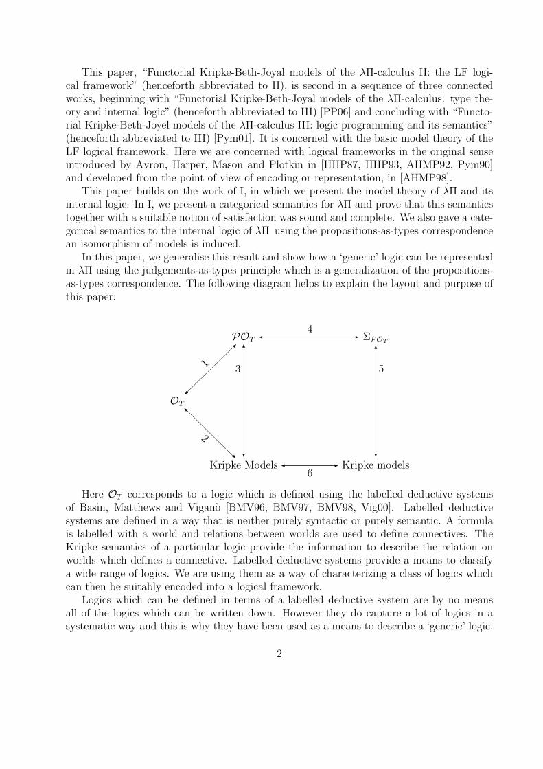
In this paper, we generalise this result and show how a ‘generic’ logic can be representedin λΠ using the judgements-as-types principle which is a generalization of the propositions-as-types correspondence. The following diagram helps to explain the layout and purpose ofthis paper:

POT�

4- ΣPOT

OT

�

1

-

Kripke Models

3

?

6

�6

-

�

2-

Kripke models

5

?

6

Here OT corresponds to a logic which is defined using the labelled deductive systemsof Basin, Matthews and Vigano [BMV96, BMV97, BMV98, Vig00]. Labelled deductivesystems are defined in a way that is neither purely syntactic or purely semantic. A formulais labelled with a world and relations between worlds are used to define connectives. TheKripke semantics of a particular logic provide the information to describe the relation onworlds which defines a connective. Labelled deductive systems provide a means to classifya wide range of logics. We are using them as a way of characterizing a class of logics whichcan then be suitably encoded into a logical framework.

Logics which can be defined in terms of a labelled deductive system are by no meansall of the logics which can be written down. However they do capture a lot of logics in asystematic way and this is why they have been used as a means to describe a ‘generic’ logic.

2

The work in this paper needs to be done in a systematic and non ad-hoc way. One way ofavoiding an ad-hoc approach is to use labelled deductive systems and this has been takenhere.

From the labelled deductive system, a proof system is extracted. This proof systemwill either be a Hilbert-type system, natural deduction system or a hybrid of the two.1

This extraction provides POT in the above diagram and we will study arrows 1 and 2.We are looking for soundness and completeness results for the correspondence 1 and theirsemantic equivalents for the correspondence 2, adequacy and faithfulness. Understandingcorrespondence 2 will allow us to see in what sense our Kripke models are related to thetraditional Kripke semantics.

So far, we have just been concerned with attempting to classify, systematically, a largerange of logics. Now, we are interested in how to encode a judged Hilbert-type system,natural deduction system or a hybrid system, POT , into LF. The correspondence 3 involvesproving soundness and completeness for a proof system obtained from a labelled deductivesystem with respect to a Kripke model. The Kripke model presented here is similar to theKripke models presented in I. We want this to be the case because we wish to consider themas objects in a category of (Kripke) models and wish to study (generalized) isomorphisms(arrows) between them.

The correspondence 4 is the encoding or representation of the object-logic in LF. Weare interested what effect the properties of the representation have on the soundness andcompleteness results for both the proof system and the encoded logic. The representationcan either be faithful or adequate. Adequacy being the strongest condition guarantees thateverything which can be proved in the proof system can be proved in the encoded systemand vice versa. State completeness induced result here

5 is the soundness and completeness result for the encoded logic. This is shown withrespect to the Kripke model presented in I. We are interested in what effect a completenessresult here has on the completeness result for POT .

Correspondence 6 is the morphism between the Kripke models for POT and the Kripkemodels for ΣOT

. We showed in I that this morphism is an isomorphism if POT is the {∀, ⊃}-fragment of minimal first-order logic and 4 was the propositions-as-types correspondence. Ingeneral we investigate what type of morphism is induced from different choices of 4.

The third paper in this sequence, “Functorial Kripke-Beth-Joyal models of the λΠ-calculus III: logic programming and its semantics” [Pym01] (henceforth abbreviated to III),provides ...

1Indeed, it seems that, [Pfe95] not withstanding, LF does not provide a satisfactory metatheory forpresentations of logical systems based on sequent calculi [Gen34].

3

2 Introduction to the LF logical framework

2.1 Introduction

In this section, we provide an introduction to the idea of logical frameworks, including boththeir logical and computational motivations.

Logically, the idea of a logical framework can be seen as arising from Martin-Lof’s intu-itionistic theory of iterated inductive definitions [ML71, ML75], in which form and inductivedefinitional status in the natural deductive rules is considered. In other words, Martin-Lofconsiders a formal metatheory of inference rules. This theory is further developed to providejustification for logical rules by extending Kant’s notion of a judgement [Kan00] in [ML82].

Computationally, the need for a formal account of the relationship between a logic andits metatheory arises from the desire, in computer science, to manipulate representationsof logics and other formal systems. Here we are mainly concerned with logics2 In order torepresent a logic to a machine, the logic must be described in a programming language ormetalogic. Moreover, if we are to understand the resulting program, we must have a fixedmechanism for describing logics in the metalogic.

2.2 The notion of a framework

In order to describe a framework, we must [IP98] have methods of:

1. Characterizing the class of (object-)logics to be represented;

2. Describing a metalogic or language, together with its metalogical status vis-a-vis theclass of object-logics;

3. Characterizing the representation mechanism.

We remark that these components are not entirely independent of each other.The above prescription can be summarized by the slogan

Framework = Language+Representaion

In § 2.3, we describe the LF logical framework, for which λΠ is the language andjudgements-as-types the representation mechanism.

2.3 The LF logical framework

In this section, we provide an overview of the LF logical framework. In the sequel, we providea detailed account of the framework from both proof-theoretic and model-theoretic pointsof view.

2Our conception of logic here is a broad one. For example, in the sequel, we shall consider the linearλ-calculus with equality judgements. Such judgements can be considered to be propositions (cf. [MM91]).

4

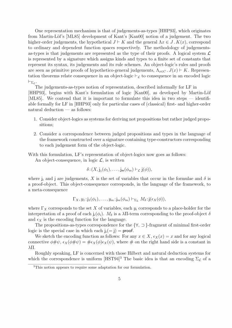
One representation mechanism is that of judgements-as-types [HHP93], which originatesfrom Martin-Lof’s [ML85] development of Kant’s [Kan00] notion of a judgement. The twohigher-order judgements, the hypothetical J ` K and the general Λx ∈ J .K(x), correspondto ordinary and dependent function spaces respectively. The methodology of judgements-as-types is that judgements are represented as the type of their proofs. A logical system Lis represented by a signature which assigns kinds and types to a finite set of constants thatrepresent its syntax, its judgements and its rule schemes. An object-logic’s rules and proofsare seen as primitive proofs of hypothetico-general judgements, Λx∈C . J(x) ` K. Represen-tation theorems relate consequence in an object-logic `L to consequence in an encoded logic`ΣL .

The judgements-as-types notion of representation, described informally for LF in[HHP93], begins with Kant’s formulation of logic [Kan00], as developed by Martin-Lof[ML85]. We contend that it is important to formulate this idea in two steps — identifi-able formally for LF in [HHP93] only for particular cases of (classical) first- and higher-ordernatural deduction — as follows:

1. Consider object-logics as systems for deriving not propositions but rather judged propo-sitions;

2. Consider a correspondence between judged propositions and types in the language ofthe framework constructed over a signature containing type-constructors correspondingto each judgement form of the object-logic.

With this formulation, LF’s representation of object-logics now goes as follows:An object-consequence, in logic L, is written

δ : (X, j1(φ1), . . . , jm(φm) `L j(φ)),

where ji and j are judgements, X is the set of variables that occur in the formulae and δ isa proof-object. This object-consequence corresponds, in the language of the framework, toa meta-consequence

ΓX , y1 : j1(φ1), . . . , ym : jm(φm) `ΣLMδ : j(εX(φ)),

where ΓX corresponds to the set X of variables, each yi corresponds to a place-holder for theinterpretation of a proof of each ji(φi). Mδ is a λΠ-term corresponding to the proof-object δand εX is the encoding function for the language.

The propositions-as-types correspondence for the {∀, ⊃}-fragment of minimal first-orderlogic is the special case in which each ji(= j) = proof.

We sketch the encoding function as follows: For any x ∈ X, εX(x) = x and for any logicalconnective φ#ψ, εX(φ#ψ) = #εX(φ)εX(ψ), where # on the right hand side is a constant inλΠ.

Roughly speaking, LF is concerned with those Hilbert and natural deduction systems forwhich the correspondence is uniform [HST94]3 The basic idea is that an encoding ΣL of a

3This notion appears to require some adaptation for our formulation.

5

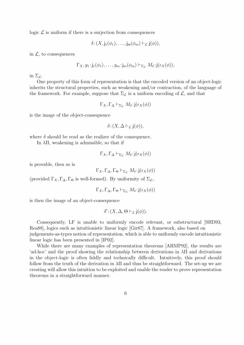
logic L is uniform if there is a surjection from consequences

δ : (X, j1(φ1), . . . , jm(φm) `L j(φ)),

in L, to consequences

ΓX , y1 : j1(φ1), . . . , ym : jm(φm) `ΣL Mδ : j(εX(φ)),

in ΣL.One property of this form of representation is that the encoded version of an object-logic

inherits the structural properties, such as weakening and/or contraction, of the language ofthe framework. For example, suppose that ΣL is a uniform encoding of L, and that

ΓX ,Γ∆ `ΣL Mδ : j(εX(φ))

is the image of the object-consequence

δ : (X,∆ `L j(φ)),

where δ should be read as the realizer of the consequence.In λΠ, weakening is admissible, so that if

ΓX ,Γ∆ `ΣL Mδ : j(εX(φ))

is provable, then so isΓX ,Γ∆,ΓΘ `ΣL Mδ : j(εX(φ))

(provided ΓX ,Γ∆,ΓΘ is well-formed). By uniformity of ΣL,

ΓX ,Γ∆,ΓΘ `ΣL Mδ : j(εX(φ))

is then the image of an object-consequence

δ′ : (X,∆,Θ `L j(φ)).

Consequently, LF is unable to uniformly encode relevant, or substructural [SHD93,Rea88], logics such as intuitionistic linear logic [Gir87]. A framework, also based onjudgements-as-types notion of representation, which is able to uniformly encode intuitionisticlinear logic has been presented in [IP02].

While there are many examples of representation theorems [AHMP92], the results are‘ad-hoc’ and the proof showing the relationship between derivations in λΠ and derivationsin the object-logic is often fiddly and technically difficult. Intuitively, this proof shouldfollow from the truth of the derivation in λΠ and thus be straightforward. The set-up we arecreating will allow this intuition to be exploited and enable the reader to prove representationtheorems in a straightforward manner.

6

3 Labelled Deductive Systems

3.1 Introduction

We wish to study the representation of the largest class of logics we can. It is by no meansclear how to write down a generic logic; in fact the question ‘what is a logic?’ is still an openproblem. To this end, we need to make a choice about the class of logics we wish to use. Inmaking this choice a lot of factors need to be taken into consideration:

• Is the characterization of the class of logics uniform?

• Are the class of logics suitable for representation in a logical framework?

• Do we capture the traditional logics, e.g. classical, intuitionistic, modal etc?

• How big is the class of logics?

It seems that our class of logics has to start with the traditional logics and providea suitable generalization of them. We also have to take into account what logics can berepresented in a logical framework; this is straightforward, the logical rules and axioms haveto give a proof system which is either Hilbert-style, natural deduction or hybrid of both.

We choose to take the labelled deductive systems of Basin, Matthews and Vigano[BMV96, BMV97, BMV98, Vig00]. This class of logics certainly describe the traditionallogics as well as providing a uniform characterization of many more. It is also the case thatthese systems have a give rise to a natural deduction proof system.

The labelled deductive systems mix semantics and syntax. The syntax comes equippedwith a Kripke semantics. To be able to represent these systems in a logical frameworkwe need to translate a labelled system into a judged system. This is done in § ??. In thissection, we are considered with defining the systems and looking at some examples of labelleddeductive systems.

The key idea behind a lablled deductive system is that connectives can be characterized bytheir relational properties, given by a Kripke semantics. To access these relational properties,each formula is labelled with a world at which it holds. It is then possible to separateconnectives into two classes; local and global.4 A local connective can only act on formulaewhich all hold at the same world while a global connective can act on formulae at differentbut related worlds.

We cannot stress enough that the choice of labelled deductive systems is just to map outa class of logics from the space of all possible logics. There are other characterizations ofclasses of logics which could have been chosen but it appears that labelled deductive systemsprovide the most suitable characterization according to the criteria set out above.

4Basin, Matthews and Vigano use non-local, but it seems that global is a better term.

7

3.2 A labelled deductive system

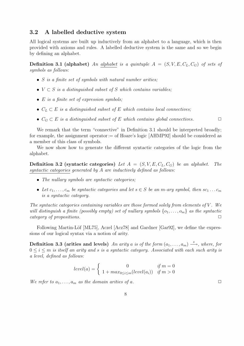
All logical systems are built up inductively from an alphabet to a language, which is thenprovided with axioms and rules. A labelled deductive system is the same and so we beginby defining an alphabet.

Definition 3.1 (alphabet) An alphabet is a quintuple A = (S, V, E,CL, CG) of sets ofsymbols as follows:

• S is a finite set of symbols with natural number arities;

• V ⊂ S is a distinguished subset of S which contains variables;

• E is a finite set of expression symbols;

• CL ⊂ E is a distinguished subset of E which contains local connectives;

• CG ⊂ E is a distinguished subset of E which contains global connectives. 2

We remark that the term “connective” in Definition 3.1 should be interpreted broadly;for example, the assignment operator := of Hoare’s logic [AHMP92] should be considered asa member of this class of symbols.

We now show how to generate the different syntactic categories of the logic from thealphabet.

Definition 3.2 (syntactic categories) Let A = (S, V, E,CL, CG) be an alphabet. Thesyntactic categories generated by A are inductively defined as follows:

• The nullary symbols are syntactic categories;

• Let c1, . . . , cm be syntactic categories and let s ∈ S be an m-ary symbol, then sc1 . . . cmis a syntactic category.

The syntactic categories containing variables are those formed solely from elements of V . Wewill distinguish a finite (possibly empty) set of nullary symbols {o1, . . . , om} as the syntacticcategory of propositions. 2

Following Martin-Lof [ML75], Aczel [Acz78] and Gardner [Gar92], we define the expres-sions of our logical syntax via a notion of arity.

Definition 3.3 (arities and levels) An arity a is of the form (a1, . . . , am)s−→, where, for

0 ≤ i ≤ m is itself an arity and s is a syntactic category. Associated with each such arity isa level, defined as follows:

level(a) =

{0 if m = 0

1 +max0≤i≤m(level(ai)) if m > 0

We refer to a1, . . . , am as the domain arities of a. 2

8

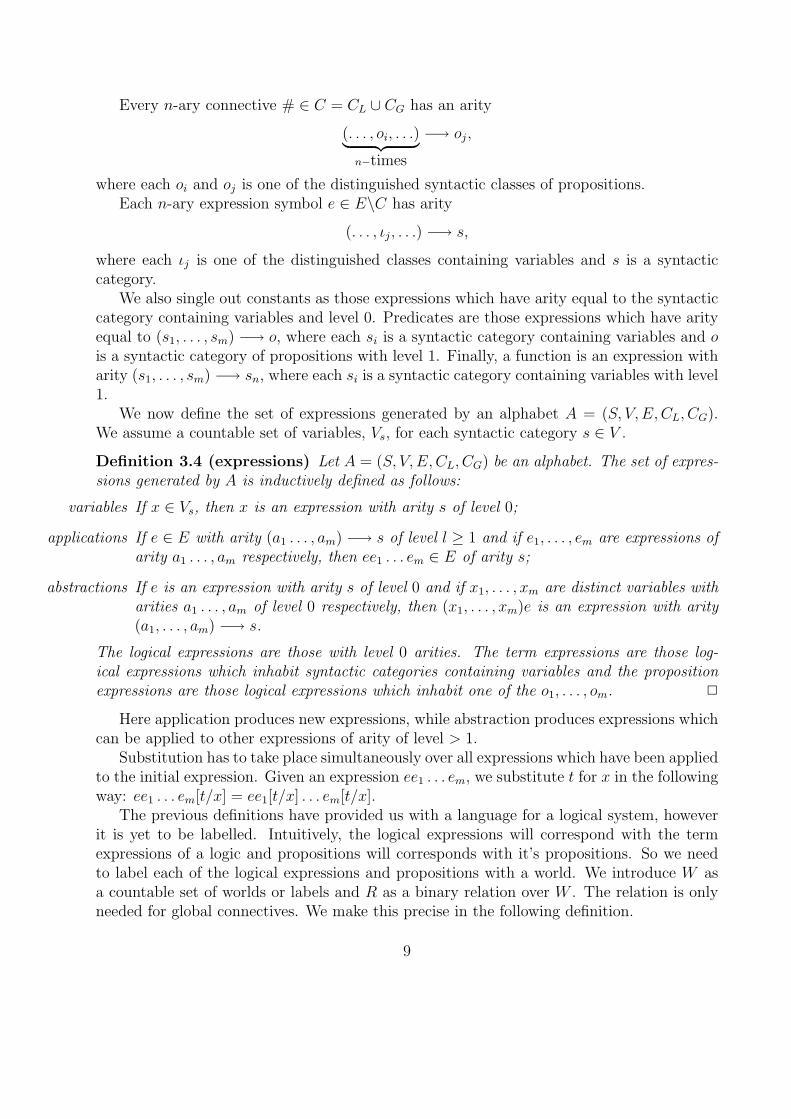
Every n-ary connective # ∈ C = CL ∪ CG has an arity

(. . . , oi, . . .)︸ ︷︷ ︸n−times

−→ oj,

where each oi and oj is one of the distinguished syntactic classes of propositions.Each n-ary expression symbol e ∈ E\C has arity

(. . . , ιj, . . .) −→ s,

where each ιj is one of the distinguished classes containing variables and s is a syntacticcategory.

We also single out constants as those expressions which have arity equal to the syntacticcategory containing variables and level 0. Predicates are those expressions which have arityequal to (s1, . . . , sm) −→ o, where each si is a syntactic category containing variables and ois a syntactic category of propositions with level 1. Finally, a function is an expression witharity (s1, . . . , sm) −→ sn, where each si is a syntactic category containing variables with level1.

We now define the set of expressions generated by an alphabet A = (S, V, E,CL, CG).We assume a countable set of variables, Vs, for each syntactic category s ∈ V .

Definition 3.4 (expressions) Let A = (S, V, E,CL, CG) be an alphabet. The set of expres-sions generated by A is inductively defined as follows:

variables If x ∈ Vs, then x is an expression with arity s of level 0;

applications If e ∈ E with arity (a1 . . . , am) −→ s of level l ≥ 1 and if e1, . . . , em are expressions ofarity a1 . . . , am respectively, then ee1 . . . em ∈ E of arity s;

abstractions If e is an expression with arity s of level 0 and if x1, . . . , xm are distinct variables witharities a1 . . . , am of level 0 respectively, then (x1, . . . , xm)e is an expression with arity(a1, . . . , am) −→ s.

The logical expressions are those with level 0 arities. The term expressions are those log-ical expressions which inhabit syntactic categories containing variables and the propositionexpressions are those logical expressions which inhabit one of the o1, . . . , om. 2

Here application produces new expressions, while abstraction produces expressions whichcan be applied to other expressions of arity of level > 1.

Substitution has to take place simultaneously over all expressions which have been appliedto the initial expression. Given an expression ee1 . . . em, we substitute t for x in the followingway: ee1 . . . em[t/x] = ee1[t/x] . . . em[t/x].

The previous definitions have provided us with a language for a logical system, howeverit is yet to be labelled. Intuitively, the logical expressions will correspond with the termexpressions of a logic and propositions will corresponds with it’s propositions. So we needto label each of the logical expressions and propositions with a world. We introduce W asa countable set of worlds or labels and R as a binary relation over W . The relation is onlyneeded for global connectives. We make this precise in the following definition.

9

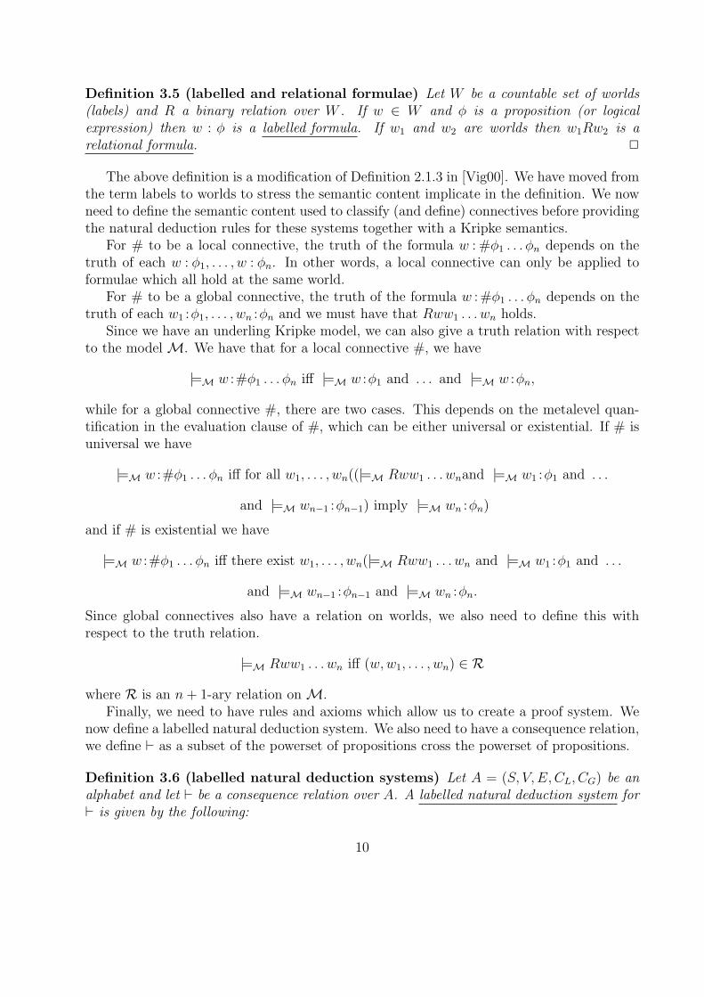
Definition 3.5 (labelled and relational formulae) Let W be a countable set of worlds(labels) and R a binary relation over W . If w ∈ W and φ is a proposition (or logicalexpression) then w : φ is a labelled formula. If w1 and w2 are worlds then w1Rw2 is arelational formula. 2

The above definition is a modification of Definition 2.1.3 in [Vig00]. We have moved fromthe term labels to worlds to stress the semantic content implicate in the definition. We nowneed to define the semantic content used to classify (and define) connectives before providingthe natural deduction rules for these systems together with a Kripke semantics.

For # to be a local connective, the truth of the formula w : #φ1 . . . φn depends on thetruth of each w : φ1, . . . , w : φn. In other words, a local connective can only be applied toformulae which all hold at the same world.

For # to be a global connective, the truth of the formula w :#φ1 . . . φn depends on thetruth of each w1 :φ1, . . . , wn :φn and we must have that Rww1 . . . wn holds.

Since we have an underling Kripke model, we can also give a truth relation with respectto the modelM. We have that for a local connective #, we have

|=M w :#φ1 . . . φn iff |=M w :φ1 and . . . and |=M w :φn,

while for a global connective #, there are two cases. This depends on the metalevel quan-tification in the evaluation clause of #, which can be either universal or existential. If # isuniversal we have

|=M w :#φ1 . . . φn iff for all w1, . . . , wn((|=M Rww1 . . . wnand |=M w1 :φ1 and . . .

and |=M wn−1 :φn−1) imply |=M wn :φn)

and if # is existential we have

|=M w :#φ1 . . . φn iff there exist w1, . . . , wn(|=M Rww1 . . . wn and |=M w1 :φ1 and . . .

and |=M wn−1 :φn−1 and |=M wn :φn.

Since global connectives also have a relation on worlds, we also need to define this withrespect to the truth relation.

|=M Rww1 . . . wn iff (w,w1, . . . , wn) ∈ R

where R is an n+ 1-ary relation onM.Finally, we need to have rules and axioms which allow us to create a proof system. We

now define a labelled natural deduction system. We also need to have a consequence relation,we define ` as a subset of the powerset of propositions cross the powerset of propositions.

Definition 3.6 (labelled natural deduction systems) Let A = (S, V, E,CL, CG) be analphabet and let ` be a consequence relation over A. A labelled natural deduction system for` is given by the following:

10

• A set of axioms;

• For each local connective # ∈ CL, an introduction rule schema of the form

...

w :φ1

[w :ψi,1] · · · [w :ψi,hi]

...

w :φi

...

w :φp#I

w :#(φ1 . . . φn)

• For each local connective # ∈ CL, an elimination rule schema of the form

w :#(φ1 . . . φn)

[Γ1]

...

w′ :χ1

· · ·

[Γp]

...

w′ :χp#e

w′ :τ

where the p minor premises of the form w :χi are derived from the set of assumptionsΓi, for 1 ≤ i ≤ p.

• For each universal global connective # ∈ CG, an introduction rule schema of the form

[w1 :φ1] · · · [wn−1 :φn−1][Rww1 . . . wn]

...

wn :φn#I

w :#φ1 . . . φn

• For each universal global connective # ∈ CG, an elimination rule schema of the form

w :#φ1 . . . φn w1 :φ1 . . . wn−1 :φn−1 Rww1 . . . wn#E

wn :φn

• For each existential global connective # ∈ CG, an introduction rule schema of the form

w1 :φ1 . . . wm :φm Rww1 . . . wm#I

w :#φ1 . . . φm

• For each existential global connective, an elimination rule schema of the form

11

w :#φ1 . . . φm

[w1 :φ1] · · · [wm :φm][Rww1 . . . wm]

...

w′ :ψ#E

w′ :ψ

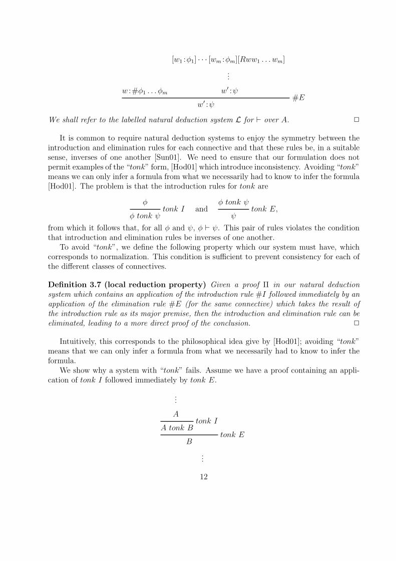
We shall refer to the labelled natural deduction system L for ` over A. 2

It is common to require natural deduction systems to enjoy the symmetry between theintroduction and elimination rules for each connective and that these rules be, in a suitablesense, inverses of one another [Sun01]. We need to ensure that our formulation does notpermit examples of the “tonk” form, [Hod01] which introduce inconsistency. Avoiding “tonk”means we can only infer a formula from what we necessarily had to know to infer the formula[Hod01]. The problem is that the introduction rules for tonk are

φtonk I

φ tonk ψand

φ tonk ψtonk E

ψ,

from which it follows that, for all φ and ψ, φ ` ψ. This pair of rules violates the conditionthat introduction and elimination rules be inverses of one another.

To avoid “tonk”, we define the following property which our system must have, whichcorresponds to normalization. This condition is sufficient to prevent consistency for each ofthe different classes of connectives.

Definition 3.7 (local reduction property) Given a proof Π in our natural deductionsystem which contains an application of the introduction rule #I followed immediately by anapplication of the elimination rule #E (for the same connective) which takes the result ofthe introduction rule as its major premise, then the introduction and elimination rule can beeliminated, leading to a more direct proof of the conclusion. 2

Intuitively, this corresponds to the philosophical idea give by [Hod01]; avoiding “tonk”means that we can only infer a formula from what we necessarily had to know to infer theformula.

We show why a system with “tonk” fails. Assume we have a proof containing an appli-cation of tonk I followed immediately by tonk E.

...

Atonk I

A tonk Btonk E

B

...

12

If we were to eliminate this step, we would not obtain a more direct proof of the conclusionsince the only way we could have proved B from A above would have been to use the “tonk”introduction and elimination rules.

So far apart from a relation on worlds, we have not really given much semantic informationto the labelled deductive system. In the definitions above, each global connective comes witha relation on worlds. The natural question is to ask how do each of these relations interact.This interaction is given by a Horn relational theory. This is a theory generated by sets ofrules of the form

Riw11 . . . w

1n · · ·Riw

m1 . . . wm

n

Riw1 . . . wn

The different rules needed for generating different modal logics come from correspondencetheory.

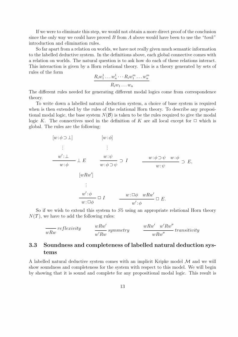
To write down a labelled natural deduction system, a choice of base system is requiredwhen is then extended by the rules of the relational Horn theory. To describe any proposi-tional modal logic, the base system N(B) is taken to be the rules required to give the modallogic K. The connectives used in the definition of K are all local except for 2 which isglobal. The rules are the following:

[w :φ⊃⊥]

...

w′ :⊥⊥ E

w :φ

[w :φ]

...

w :ψ⊃ I

w :φ⊃ψw :φ⊃ψ w :φ

⊃ E,w :ψ

[wRw′]

...

w′ :φ2 I

w :2φ

w :2φ wRw′

2 E.w′ :φ

So if we wish to extend this system to S5 using an appropriate relational Horn theoryN(T ), we have to add the following rules:

reflexivitywRw

wRw′

symmetryw′Rw

wRw′ w′Rw′′

transitivitywRw′′

3.3 Soundness and completeness of labelled natural deduction sys-tems

A labelled natural deductive system comes with an implicit Kripke model M and we willshow soundness and completeness for the system with respect to this model. We will beginby showing that it is sound and complete for any propositional modal logic. This result is

13

taken straight from [Vig00] and we consider a base system N(K) as defined above togetherwith a relational Horn theory N(T ). We only sketch the main details of the results, we donot deal with the case where Skolem functions are involved. To deal with this case, we needto extend Definition 3.8 to include constants which will deal with Skolem functions and wealso need to consider the Horn relational theory as corresponding to a collection of restrictedconvergency axioms. The details for this can be found in [Vig00]. We present the soundnessand completeness to demonstrate that the labelled natural deductive systems do characterizea sensible class of logics.

We follow [Vig00] and start by defining a Kripke frame for our propositional modal logicN(L).

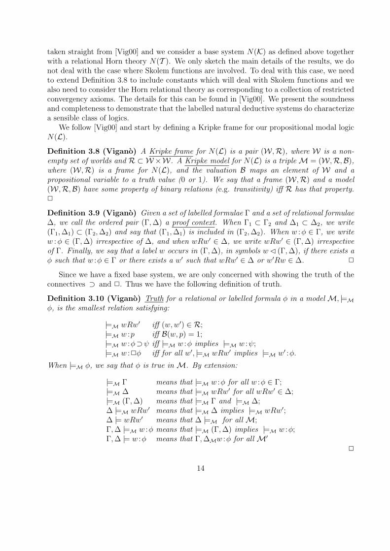
Definition 3.8 (Vigano) A Kripke frame for N(L) is a pair (W ,R), where W is a non-empty set of worlds and R ⊂ W×W. A Kripke model for N(L) is a tripleM = (W ,R,B),where (W ,R) is a frame for N(L), and the valuation B maps an element of W and apropositional variable to a truth value (0 or 1). We say that a frame (W ,R) and a model(W ,R,B) have some property of binary relations (e.g. transitivity) iff R has that property.2

Definition 3.9 (Vigano) Given a set of labelled formulae Γ and a set of relational formulae∆, we call the ordered pair (Γ,∆) a proof context. When Γ1 ⊂ Γ2 and ∆1 ⊂ ∆2, we write(Γ1,∆1) ⊂ (Γ2,∆2) and say that (Γ1,∆1) is included in (Γ2,∆2). When w :φ ∈ Γ, we writew :φ ∈ (Γ,∆) irrespective of ∆, and when wRw′ ∈ ∆, we write wRw′ ∈ (Γ,∆) irrespectiveof Γ. Finally, we say that a label w occurs in (Γ,∆), in symbols w� (Γ,∆), if there exists aφ such that w :φ ∈ Γ or there exists a w′ such that wRw′ ∈ ∆ or w′Rw ∈ ∆. 2

Since we have a fixed base system, we are only concerned with showing the truth of theconnectives ⊃ and 2. Thus we have the following definition of truth.

Definition 3.10 (Vigano) Truth for a relational or labelled formula φ in a modelM, |=Mφ, is the smallest relation satisfying:

|=M wRw′ iff (w,w′) ∈ R;|=M w :p iff B(w, p) = 1;|=M w :φ⊃ψ iff |=M w :φ implies |=M w :ψ;|=M w :2φ iff for all w′, |=M wRw′ implies |=M w′ :φ.

When |=M φ, we say that φ is true in M. By extension:

|=M Γ means that |=M w :φ for all w :φ ∈ Γ;|=M ∆ means that |=M wRw′ for all wRw′ ∈ ∆;|=M (Γ,∆) means that |=M Γ and |=M ∆;∆ |=M wRw′ means that |=M ∆ implies |=M wRw′;∆ |= wRw′ means that ∆ |=M for all M;Γ,∆ |=M w :φ means that |=M (Γ,∆) implies |=M w :φ;Γ,∆ |= w :φ means that Γ,∆Mw :φ for all M′

2

14

The truth relation above is the same as the usual truth function for modal logics if weremove the world label and consider the relation as being true at a particular world.

We are now in a position to state and prove the soundness result for labelled propositionalmodal logics.

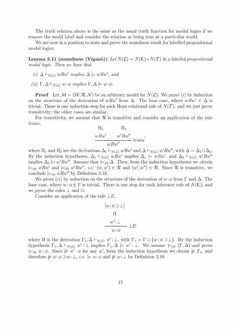
Lemma 3.11 (soundness (Vigano)) Let N(L) = N(K)+N(T ) be a labelled propositionalmodal logic. Then we have that

(i) ∆ `N(L) wRw′ implies ∆ |= wRw′, and

(ii) Γ,∆ `N(L) w :φ implies Γ,∆ |= w :φ.

Proof LetM = (W ,R,N ) be an arbitrary model for N(L). We prove (i) by inductionon the structure of the derivation of wRw′ from ∆. The base case, where wRw′ ∈ ∆ istrivial. There is one induction step for each Horn relational rule of N(T ), and we just provetransitivity; the other cases are similar.

For transitivity, we assume that R is transitive and consider an application of the ruletrans,

Π1

wRw′

Π2

w′Rw′′

transwRw′′

,

where Π1 and Π2 are the derivations ∆1 `N(L) wRw′ and ∆ `N(L) w

′Rw′′, with ∆ = ∆1∪∆2.By the induction hypotheses, ∆1 `N(L) wRw

′ implies ∆1 |= wRw′, and ∆2 `N(L) w′Rw′′

implies ∆2 |= w′Rw′′. Assume that |=M ∆. Then, from the induction hypotheses we obtain|=M wRw′ and |=M w′Rw′′, i.e. (w,w′) ∈ R and (w′, w′′) ∈ R. Since R is transitive, weconclude |=M wRw′′ by Definition 3.10.

We prove (ii) by induction on the structure of the derivation of w :φ from Γ and ∆. Thebase case, where w :φ ∈ Γ is trivial. There is one step for each inference rule of N(K), andwe prove the rules ⊥ and 2.

Consider an application of the rule ⊥E,

[w :φ⊃⊥]

Π

w′ :⊥⊥E

w :φ

where Π is the derivation Γ1,∆ `N(L) w′ :⊥, with Γ1 = Γ ∪ {w : φ⊃⊥}. By the induction

hypothesis Γ1,∆ `N(L) w′ : ⊥ implies Γ1,∆ |= w′ : ⊥. We assume |=M (Γ,∆) and prove

|=M w : φ. Since 6|= w′ : φ for any w′, form the induction hypothesis we obtain 6|= Γ1, andtherefore 6|= w :φ⊃w :⊥, i.e. |= w :φ and 6|= w :⊥ by Definition 3.10.

15

Consider an application of the rule ⊃ I,

[w :φ]

Π

w :ψ⊃ I

w :φ⊃ψ

where Π is the derivation Γ1,∆ `N(L) w : ψ, with Γ1 = Γ ∪ {w : φ}. By the inductionhypothesis, Γ1,∆ `N(L) w :φ implies Γ1,∆ |= w :φ. Assume |=M (Γ,∆). Since 6|=M w :ψ forany w, from the induction hypothesis 6|=M Γ1, and therefore 6|=M w :φ, i.e. |=M w :φ⊃ψ byDefinition 3.10.

Consider an application of the rule ⊃E,

Π1

w :φ⊃ψ

Π2

w :φ⊃E

w :ψ

where Π1 and Π2 are the derivations Γ1,∆ `N(L) w : φ⊃ψ and Γ2,∆ `N(L) w : φ, withΓ = Γ1 ∪ Γ2. By the induction hypotheses, Γ1,∆ `N(L) w :φ⊃ψ implies Γ1,∆ |= w :φ⊃ψand Γ2,∆ `N(L) w : φ implies Γ2,∆ |= w : φ. We assume |=M (Γ,∆). From the inductionhypotheses, we have that |=M w :φ⊃ψ and |=M w :ψ and thus |=M w :ψ by Definition 3.10.

Consider an application of the rule 2I,

[wRw′]

Π

w′ :φ2I

w :2φ

where Π is the derivation Γ,∆1 `N(L) w′ : φ, with ∆1 = ∆ ∪ {wRw′}. By the induction

hypothesis, Γ,∆1 `N(L) w′ : φ implies Γ,∆1 |= w′ : φ. Assume |=M (Γ,∆). Considering

the restriction on the application of 2I, we can extend ∆ to ∆′ = ∆ ∪ {wRw′′} for anarbitrary w′′ 6�(Γ,∆), and assume |=M ∆′. Since |=M ∆′ implies |=M ∆1, from the inductionhypothesis we obtain |=M w′ : φ, that is |=M w′′ : φ for an arbitrary w′′ 6�(Γ, δ) such that|=M wRw′′. We conclude |=M w :2φ by Definition 3.10.

Consider an application of the rule 2E,

Π1

w :2φ

Π2

wRw′

2Ew′ :φ

where Π1 and Π2 are the derivations Γ,∆1 `N(L) w : 2φ and ∆2 `N(L) wRw′, with ∆ =

∆1 ∪ ∆2. Assume |=M (Γ, δ). Then, from the induction hypotheses we obtain |=M w : 2φand |=M wRw′, and thus |=M w′ :φ by Definition 3.10. 2

16

Before we can move on to completeness for a labelled propositional modal logic a fewmore definitions and results are needed. The proof of completeness follows a Henkin-styleproof an so we need to have a definition of a maximally consistent extension of our proofcontext. We does this in the usual way.

Definition 3.12 (Vigano) Let N(L) = N(K) +N(T ) be consistent system, i. e. 6`N(L) w :⊥ for every w. A proof context (Γ,∆) is N(L)-consistent iff Γ,∆ 6`N(L) w :⊥ for every w.(Γ,∆) is N(L)-inconsistent iff it is not N(L)-consistent. 2

We will abuse by notation by talking about consistent and inconsistent proof contexts ingeneral rather than N(L)-consistent and inconsistent proof contexts. To keep the notationdown, we introduce negation, which is defined as follows:

|=M w :¬φ iff 6|=M w :φiff |=M w :φ implies |=M w :⊥

with inference rules[w :φ]

...

w :⊥¬ I

w :¬φw :¬φ w :φ

¬Ew :⊥

this is a derived rule from N(K) and so we can just add it to the system without worryingabout loss of soundness. We can now formulate the following result for labelled propositionalmodal logics.

Proposition 3.13 (Vigano) If (Γ,∆) is consistent, then for every w and every φ, either(Γ ∪ {w :φ},∆) is consistent or (Γ ∪ {¬φ},∆) is consistent.

We now define the deductive closure of the relational Horn theory,

Definition 3.14 (Vigano) Let N(L) = N(K) + N(T ) be a labelled propositional modallogic, let ∆N(L) be the deductive closure of ∆ under N(L), i.e.

∆N(L) =def {wRw′|∆ `N(L) wRw′}.

2

From this definition and Proposition 3.13, we can deduce thatΓ,∆ `N(L) φ iff Γ,∆N(L) `N(L) φ, and that ∆N(L) might be empty when ∆ is empty and forexample, N(L) is N(K).

Definition 3.15 (Vigano) A proof context (Γ,∆) is maximally consistent iff

17

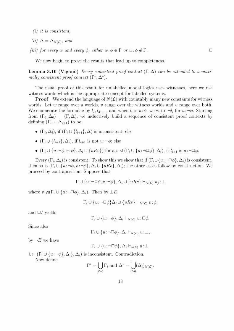
(i) it is consistent,

(ii) ∆ = ∆N(L), and

(iii) for every w and every φ, either w :φ ∈ Γ or w :φ 6∈ Γ. 2

We now begin to prove the results that lead up to completeness.

Lemma 3.16 (Vigano) Every consistent proof context (Γ,∆) can be extended to a maxi-mally consistent proof context (Γ∗,∆∗).

The usual proof of this result for unlabelled modal logics uses witnesses, here we usewitness words which is the appropriate concept for labelled systems.

Proof We extend the language of N(L) with countably many new constants for witnessworlds. Let w range over a worlds, v range over the witness worlds and u range over both.We enumerate the formulae by l1, l2, . . . and when li is u :φ, we write ¬li for u :¬φ. Startingfrom (Γ0,∆0) = (Γ,∆), we inductively build a sequence of consistent proof contexts bydefining (Γi+1,∆i+1) to be:

• (Γi,∆i), if (Γi ∪ {li+1},∆) is inconsistent; else

• (Γi ∪ {li+1},∆i), if li+1 is not u :¬φ; else

• (Γi ∪ {u :¬φ, v :φ},∆i ∪ {uRv}) for a v � (Γi ∪ {u :¬2φ},∆i), if li+1 is u :¬2φ.

Every (Γi,∆i) is consistent. To show this we show that if (Γi∪{u :¬2φ},∆i) is consistent,then so is (Γi ∪ {u :¬φ, v :¬φ},∆i ∪ {uRv},∆i); the other cases follow by construction. Weproceed by contraposition. Suppose that

Γ ∪ {u :¬2φ, v :¬φ},∆i ∪ {uRv} `N(L) uj :⊥

where v 6�(Γi ∪ {u :¬2φ},∆i). Then by ⊥E,

Γi ∪ {u :¬2φ}∆i ∪ {uRv} `N(L) v :φ,

and 2I yieldsΓi ∪ {u :¬φ},∆i `N(L) u :2φ.

Since alsoΓi ∪ {u :¬2φ},∆i `N(L) u :⊥,

by ¬E we haveΓi ∪ {u :¬2φ},∆i `n(L) u :⊥,

i.e. (Γi ∪ {u :¬φ},∆i},∆i) is inconsistent. Contradiction.Now define

Γ∗ =⋃i≥0

Γi and ∆∗ =⋃i≥0

(∆i)N(L).

18

We show that (Γ∗,∆∗) is maximally consistent by proving that it satisfies the conditions inDefinition 3.15. For (i), note that

if (⋃i≥0

Γi,⋃i≥0

∆i) is consistent, then so is (⋃i≥0

Γi,⋃i≥0

(∆i)N(L)).

Now suppose that (Γ∗,∆∗) is inconsistent. Then for some finite (Γ′,∆′) included in (Γ∗,∆∗)there exists a u such that Γ′,∆′ `N(L) u : ⊥. Every labelled formulae l ∈ (Γ′,∆′) is insome (Γj,∆j). For each l ∈ (Γ′,∆′), let il be the least j such that l ∈ (Γj,∆j) and i =max{il|l ∈ (Γ′,∆′)}. Then (Γ′,∆′) ⊂ (Γi,∆i), and (Γi,∆i) is inconsistent, which is not thecase. Condition (ii) is satisfied by the definition of ∆∗. For (iii), suppose that li+1 /∈ (Γ∗,∆∗).Then li+1 /∈ (Γi+1,∆i+1) and (Γi ∪ {li+1},∆i) is inconsistent. Thus, by Proposition 3.13,(Γi ∪ {¬li+1,∆i) is consistent, and ¬li+1 is consistently added to some (Γj,∆j) during theconstruction, and therefore ¬li+1 ∈ (Γ∗,∆∗). 2

We now state and prove some properties of maximally consistent proof contexts.

Proposition 3.17 (Vigano) Let (Γ∗,∆∗) be a maximally consistent proof context. Then

(i) ∆∗ `N(L) uiRuj iff uiRuj ∈ ∆∗.

(ii) Γ∗,∆∗ `N(L) u :φ iff u :φ ∈ Γ∗.

(iii) u :φ⊃ψ ∈ Γ∗ iff u :φ ∈ Γ∗ implies u :ψ ∈ Γ∗.

(iv) ui :2φ ∈ Γ∗ iff uiRuj ∈ ∆∗ implies uj :φ ∈ Γ∗ for all uj.

Proof (i) and (ii) follow immediately by definition and Proposition 3.13. We only prove(iv); (v) follows analogously. From left-to-right direction, suppose that ui :2φ ∈ Γ∗. Then,by (iii), Γ∗,∆∗ `N(L) ui :2φ, and, by 2E, we have ∆∗ `N(L) uiRuj implies Γ∗,∆∗ `N(L) uj :φfor all uj. By (i) and (ii), conclude that uiRuj ∈ ∆∗ implies uj :φ ∈ Γ∗ for all uj. For theconverse, suppose that ui :2φ /∈ Γ∗. Then ui :2φ ∈ Γ∗, and, by the construction of (Γ∗,∆∗),there exists a uj such that uiRuj ∈ ∆∗ and uj :φ ∈ Γ∗. 2

We are now in a position to define the canonical model.

Definition 3.18 (Viagno) Given a maximally consistent proof context (Γ∗,∆∗), we definethe canonical model MC = (WC ,RC ,BC) for the proof system N(L) as follows:

• WC = {u|u� (Γ∗,∆∗)};

• (ui, uj) ∈ RC iff uiRuj ∈ ∆∗;

• BC(u, p) = 1 iff u :p ∈ Γ∗. 2

We now have two more propositions and then we get completeness.

Proposition 3.19 (Vigano) uiRuj ∈ ∆∗ iff ∆∗ |=MC uiRuj.

19

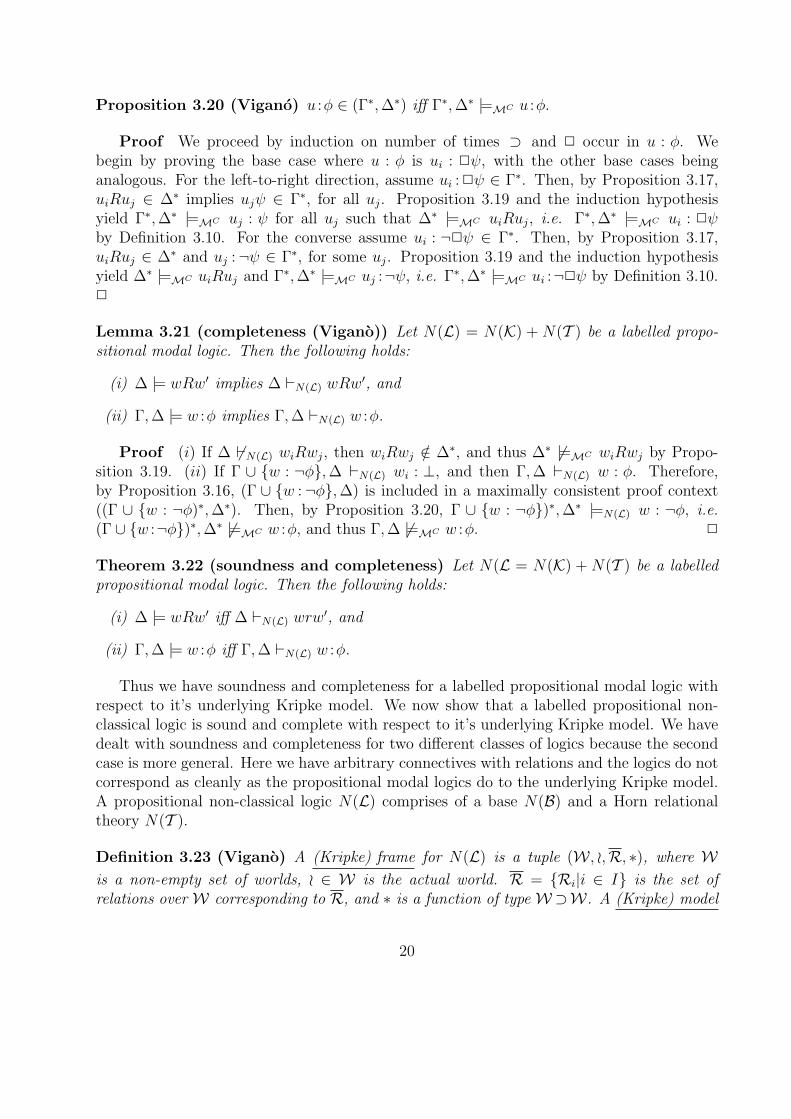
Proposition 3.20 (Vigano) u :φ ∈ (Γ∗,∆∗) iff Γ∗,∆∗ |=MC u :φ.

Proof We proceed by induction on number of times ⊃ and 2 occur in u : φ. Webegin by proving the base case where u : φ is ui : 2ψ, with the other base cases beinganalogous. For the left-to-right direction, assume ui :2ψ ∈ Γ∗. Then, by Proposition 3.17,uiRuj ∈ ∆∗ implies ujψ ∈ Γ∗, for all uj. Proposition 3.19 and the induction hypothesisyield Γ∗,∆∗ |=MC uj : ψ for all uj such that ∆∗ |=MC uiRuj, i.e. Γ∗,∆∗ |=MC ui : 2ψby Definition 3.10. For the converse assume ui : ¬2ψ ∈ Γ∗. Then, by Proposition 3.17,uiRuj ∈ ∆∗ and uj :¬ψ ∈ Γ∗, for some uj. Proposition 3.19 and the induction hypothesisyield ∆∗ |=MC uiRuj and Γ∗,∆∗ |=MC uj :¬ψ, i.e. Γ∗,∆∗ |=MC ui :¬2ψ by Definition 3.10.2

Lemma 3.21 (completeness (Vigano)) Let N(L) = N(K) + N(T ) be a labelled propo-sitional modal logic. Then the following holds:

(i) ∆ |= wRw′ implies ∆ `N(L) wRw′, and

(ii) Γ,∆ |= w :φ implies Γ,∆ `N(L) w :φ.

Proof (i) If ∆ 6`N(L) wiRwj, then wiRwj /∈ ∆∗, and thus ∆∗ 6|=MC wiRwj by Propo-sition 3.19. (ii) If Γ ∪ {w : ¬φ},∆ `N(L) wi : ⊥, and then Γ,∆ `N(L) w : φ. Therefore,by Proposition 3.16, (Γ ∪ {w :¬φ},∆) is included in a maximally consistent proof context((Γ ∪ {w : ¬φ)∗,∆∗). Then, by Proposition 3.20, Γ ∪ {w : ¬φ})∗,∆∗ |=N(L) w : ¬φ, i.e.(Γ ∪ {w :¬φ})∗,∆∗ 6|=MC w :φ, and thus Γ,∆ 6|=MC w :φ. 2

Theorem 3.22 (soundness and completeness) Let N(L = N(K) + N(T ) be a labelledpropositional modal logic. Then the following holds:

(i) ∆ |= wRw′ iff ∆ `N(L) wrw′, and

(ii) Γ,∆ |= w :φ iff Γ,∆ `N(L) w :φ.

Thus we have soundness and completeness for a labelled propositional modal logic withrespect to it’s underlying Kripke model. We now show that a labelled propositional non-classical logic is sound and complete with respect to it’s underlying Kripke model. We havedealt with soundness and completeness for two different classes of logics because the secondcase is more general. Here we have arbitrary connectives with relations and the logics do notcorrespond as cleanly as the propositional modal logics do to the underlying Kripke model.A propositional non-classical logic N(L) comprises of a base N(B) and a Horn relationaltheory N(T ).

Definition 3.23 (Vigano) A (Kripke) frame for N(L) is a tuple (W , o,R, ∗), where Wis a non-empty set of worlds, o ∈ W is the actual world. R = {Ri|i ∈ I} is the set ofrelations over W corresponding to R, and ∗ is a function of type W⊃W. A (Kripke) model

20

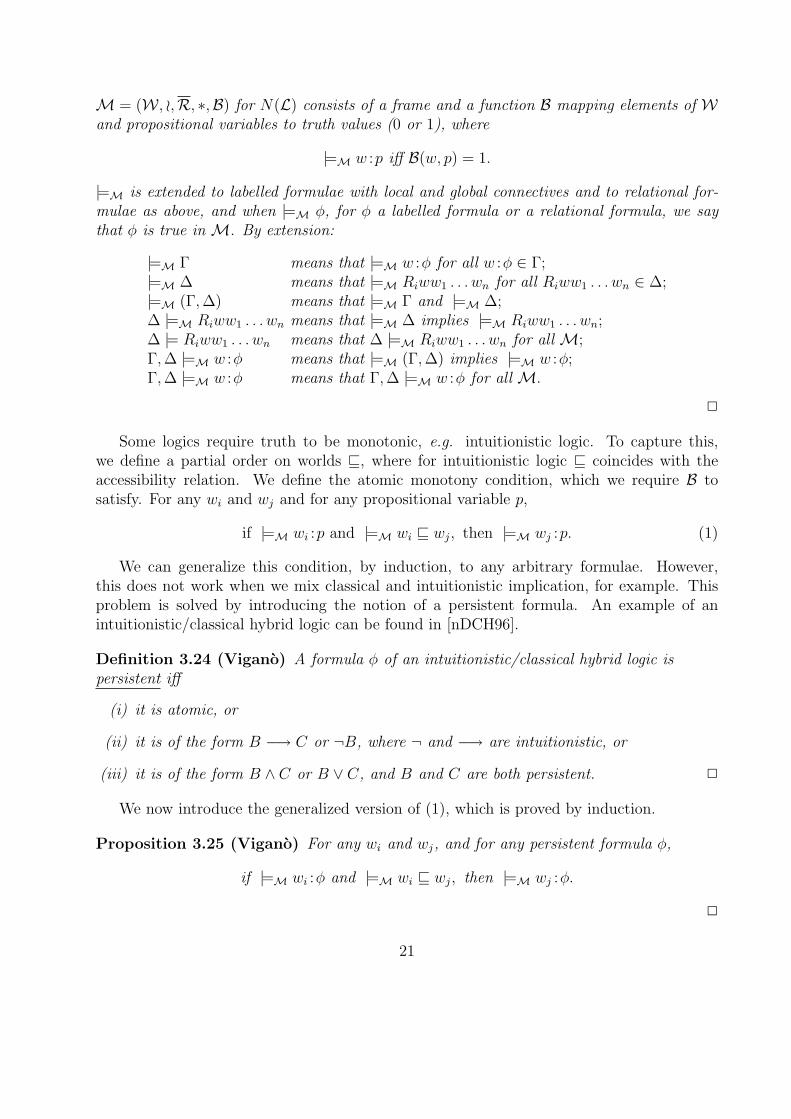
M = (W , o,R, ∗,B) for N(L) consists of a frame and a function B mapping elements of Wand propositional variables to truth values (0 or 1), where

|=M w :p iff B(w, p) = 1.

|=M is extended to labelled formulae with local and global connectives and to relational for-mulae as above, and when |=M φ, for φ a labelled formula or a relational formula, we saythat φ is true in M. By extension:

|=M Γ means that |=M w :φ for all w :φ ∈ Γ;|=M ∆ means that |=M Riww1 . . . wn for all Riww1 . . . wn ∈ ∆;|=M (Γ,∆) means that |=M Γ and |=M ∆;∆ |=M Riww1 . . . wn means that |=M ∆ implies |=M Riww1 . . . wn;∆ |= Riww1 . . . wn means that ∆ |=M Riww1 . . . wn for all M;Γ,∆ |=M w :φ means that |=M (Γ,∆) implies |=M w :φ;Γ,∆ |=M w :φ means that Γ,∆ |=M w :φ for all M.

2

Some logics require truth to be monotonic, e.g. intuitionistic logic. To capture this,we define a partial order on worlds v, where for intuitionistic logic v coincides with theaccessibility relation. We define the atomic monotony condition, which we require B tosatisfy. For any wi and wj and for any propositional variable p,

if |=M wi :p and |=M wi v wj, then |=M wj :p. (1)

We can generalize this condition, by induction, to any arbitrary formulae. However,this does not work when we mix classical and intuitionistic implication, for example. Thisproblem is solved by introducing the notion of a persistent formula. An example of anintuitionistic/classical hybrid logic can be found in [nDCH96].

Definition 3.24 (Vigano) A formula φ of an intuitionistic/classical hybrid logic ispersistent iff

(i) it is atomic, or

(ii) it is of the form B −→ C or ¬B, where ¬ and −→ are intuitionistic, or

(iii) it is of the form B ∧ C or B ∨ C, and B and C are both persistent. 2

We now introduce the generalized version of (1), which is proved by induction.

Proposition 3.25 (Vigano) For any wi and wj, and for any persistent formula φ,

if |=M wi :φ and |=M wi v wj, then |=M wj :φ.

2

21

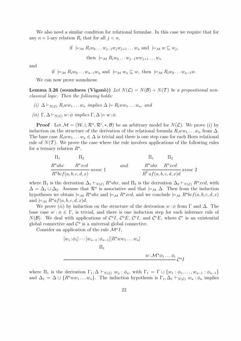
We also need a similar condition for relational formulae. In this case we require that forany n+ 1-ary relation Ri that for all j < n,

if |=M Riw0 . . . wj−1wjwj+1 . . . wn and |=M w v wj,

then |=M Riw0 . . . wj−1wwj+1 . . . wn

andif |=M Riw0 . . . wn−1wn and |=M wn v w, then |=M Riw0 . . . wn−1w.

We can now prove soundness:

Lemma 3.26 (soundness (Vigano)) Let N(L) = N(B) + N(T ) be a propositional non-classical logic. Then the following holds:

(i) ∆ `N(L) Riww1 . . . wn implies ∆ |= Riww1 . . . wn, and

(ii) Γ,∆ `N(L) w :φ implies Γ,∆ |= w :φ.

Proof Let M = (W , o,Ru,Re, ∗,B) be an arbitrary model for N(L). We prove (i) byinduction on the structure of the derivation of the relational formula Riww1 . . . wn from ∆.The base case Riww1 . . . wn ∈ ∆ is trivial and there is one step case for each Horn relationalrule of N(T ). We prove the case where the rule involves applications of the following rulesfor a ternary relation Ru,

Π1

Ruabx

Π2

Ruxcdassoc 1

Rubcf(a, b, c, d, x)

and

Π1

Ruabx

Π2

Ruxcdassoc 2

RUaf(a, b, c, d, x)d

where Π1 is the derivation ∆1 `N(L) Ruabx, and Π2 is the derivation ∆2 `N(L) R

uxcd, with∆ = ∆1 ∪ ∆2. Assume that Ru is associative and that |=M ∆. Then from the inductionhypotheses we obtain |=M Ruabx and |=M Ruxcd, and we conclude |=M Rubcf(a, b, c, d, x)and |=M Ruaf(a, b, c, d, x)d.

We prove (ii) by induction on the structure of the derivation w :φ from Γ and ∆. Thebase case w : φ ∈ Γ, is trivial, and there is one induction step for each inference rule ofN(B). We deal with applications of CuI, CuE, CeI, and CeE, where Ce is an existentialglobal connective and Cu is a universal global connective.

Consider an application of the ruleMuI,

[w1 :φ1] · · · [wu−1 :φu−1][Ruww1 . . . wu]

Π1

w :Muφ1 . . . φiCuI

where Π1 is the derivation Γ1,∆ `N(L) wu : φu, with Γ1 = Γ ∪ {w1 : φ1, . . . , wu−1 : φu−1}and ∆1 = ∆ ∪ {Ruww1 . . . wn}. The induction hypothesis is Γ1,∆1 `N(L) wu : φu implies

22

Γ1,∆1 |= wu :φu. Assume |=M (Γ,∆). Considering the restriction on the application ofMuI,we can extend Γ and ∆ to Γ′ = Γ ∪ {w′1 :φ1, . . . , w

′u−1 :φu−1} and ∆′ = ∆ ∪ {Ruww′1 . . . w

′u}

for arbitrary w′1, . . . , w′u 6�(Γ,∆), and assume |=M Γ′ and |=M ∆′. Since |=M Γ′ implies

|=M Γ1 and |=M ∆′ implies |=M ∆1, from the induction hypothesis we obtain |=M w′u :φu forarbitrary w′1, . . . , w

′u 6�(Γ,∆) such that |=M Ruww′1 . . . w

′u and |=M w′1 : φ1, . . . , |=M w′u−1 :

φu−1. We conclude |=M w :Cuφ1 . . . φu from the definition of |=M.Consider a application of the rule CuE,

Π0

w :Cuφ1 . . . φu

Π1

w1 :φ1 · · ·

Πu−1

wu−1 :φu−1

Πu

Ruww1 . . . wuCuE

wu :φu

where Π0 is the derivation Γ0,∆0 `N(L) w :Cuφ1 . . . φu; Πi is the derivation Γi,∆i `N(L) wi :φi;Πu is the derivation ∆u `N(L) R

uww1 . . . wu; Γ =⋃

0≤i≤u Γi and ∆ =⋃

0≤i≤n ∆i. Assume|=M (Γ,∆). Then, from the induction hypotheses we obtain |=M w : Cuφ1 . . . φu, |=M w1 :φ1, . . . , |=M wu−1 :φu−1, and |=M Ruww1 . . . wu, and thus |=M wu :φu from the definition of|=M.

Consider an application of the rule CeI,

Π1

w1 :φ1 · · ·

Πe

we :φe

Πe+1

Reww1 . . . weCeI

w :Ceφ1 . . . φe

where Πi is the derivation Γi,∆i `N(L) wi :φi, for 1 ≤ i ≤ e; Πe+1 is the derivation ∆e+1 `N(L)

Reww1 . . . we; Γ =⋃

1≤i≤e Γi and ∆ =⋃

1≤i≤e+1 ∆i. Assume |=M (Γ,∆). Then, from theinduction hypotheses we obtain |=M w1 :φ1, . . . , |=M we :φe and |=M Reww1 . . . we, and thus|=M w :Ceφ1 . . . φe from the definition of |=M.

For CeE, let Π be the derivation

Π1

w :Ceφ1 . . . φe

[w1 :φ1] · · · [we :φe][Reww1 . . . we]

Π2

y :ψCeE

y :ψ

That is, Π is Γ,∆ `N(L) y :ψ, where, by the restriction on CeE, the labels w1, . . . , we do notoccur in (Γ,∆) and are different from w and y. Moreover, Π1 is the derivation Γ,∆ `N(L)

w : Ceφ1 . . . φe, and Π2 is the derivation Γ ∪ {w1 : φ1, . . . , we : φe},∆ ∪ {Reww1 . . . we} `N(L)

w′ : ψ. By the induction hypothesis for Π1, we have that Γ,∆ |=M w : Ceφ1 . . . φe, andthus, from the definition of |=M, there exist y1, . . . , ye such that |=M y1 :φ1, . . . , |=M ye :φe

and |=M Rewy1 . . . ye. We can extend Γ and ∆ to Γ′ = Γ ∪ {w′1 : φ1, . . . , w′e : φe} and

∆′ = ∆∪{Reww′1 . . . w′e} for arbitrary w′1, . . . , w

′e 6�(Γ,∆), and from the induction hypothesis

for Π2 we conclude Γ,∆ |=M y :ψ. 2

23

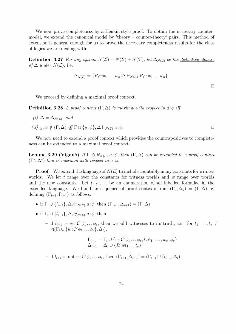
We now prove completeness by a Henkin-style proof. To obtain the necessary counter-model, we extend the canonical model by ’theory – counter-theory‘ pairs. This method ofextension is general enough for us to prove the necessary completeness results for the classof logics we are dealing with.

Definition 3.27 For any system N(L) = N(B) +N(T ), let ∆N(L) be the deductive closureof ∆ under N(L), i.e.

∆N(L) = {Riww1 . . . wn|∆ `N(L) Riww1 . . . wn}.

2

We proceed by defining a maximal proof context.

Definition 3.28 A proof context (Γ,∆) is maximal with respect to a :φ iff

(i) ∆ = ∆N(L), and

(ii) y :ψ /∈ (Γ,∆) iff Γ ∪ {y :ψ},∆ `N(L) a :φ. 2

We now need to extend a proof context which provides the countrapositives to complete-ness can be extended to a maximal proof context.

Lemma 3.29 (Vigano) If Γ,∆ 6`N(L) a :φ, then (Γ,∆) can be extended to a proof context(Γ∗,∆∗) that is maximal with respect to a :φ.

Proof We extend the language ofN(L) to include countably many constants for witnessworlds. We let t range over the constants for witness worlds and w range over worldsand the new constants. Let l1, l2, . . . be an enumeration of all labelled formulae in theextended language. We build an sequence of proof contexts from (Γ0,∆0) = (Γ,∆) bydefining (Γi+1,Γi+1) as follows:

• if Γi ∪ {li+1},∆i `N(L) a :φ, then (Γi+1,∆i+1) = (Γ,∆)

• if Γi ∪ {li+1},∆i 6`N(L) a :φ, then

– if li+1 is w : Ceφ1 . . . φe, then we add witnesses to its truth, i.e. for t1, . . . , te 6�(Γi ∪ {w :Ceφ1 . . . φe},∆i),

Γi+1 = Γi ∪ {w :Ceφ1 . . . φe, t :φ1, . . . , we :φe}∆i+1 = ∆i ∪ {Rewt1 . . . te}

– if li+1 is not w :Ceφ1 . . . φe, then (Γi+1,∆i+1) = (Γi+1 ∪ {li+1,∆i)

24

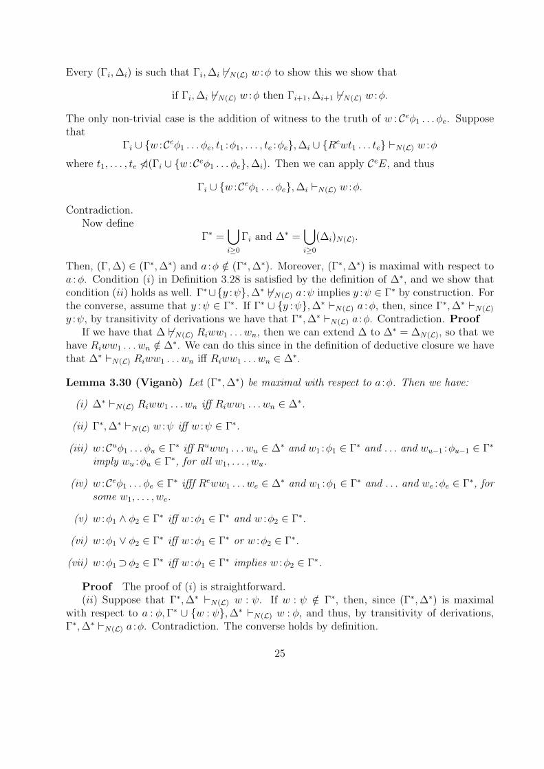
Every (Γi,∆i) is such that Γi,∆i 6`N(L) w :φ to show this we show that

if Γi,∆i 6`N(L) w :φ then Γi+1,∆i+1 6`N(L) w :φ.

The only non-trivial case is the addition of witness to the truth of w : Ceφ1 . . . φe. Supposethat

Γi ∪ {w :Ceφ1 . . . φe, t1 :φ1, . . . , te :φe},∆i ∪ {Rewt1 . . . te} `N(L) w :φ

where t1, . . . , te 6�(Γi ∪ {w :Ceφ1 . . . φe},∆i). Then we can apply CeE, and thus

Γi ∪ {w :Ceφ1 . . . φe},∆i `N(L) w :φ.

Contradiction.Now define

Γ∗ =⋃i≥0

Γi and ∆∗ =⋃i≥0

(∆i)N(L).

Then, (Γ,∆) ∈ (Γ∗,∆∗) and a :φ /∈ (Γ∗,∆∗). Moreover, (Γ∗,∆∗) is maximal with respect toa :φ. Condition (i) in Definition 3.28 is satisfied by the definition of ∆∗, and we show thatcondition (ii) holds as well. Γ∗∪{y :ψ},∆∗ 6`N(L) a :ψ implies y :ψ ∈ Γ∗ by construction. Forthe converse, assume that y :ψ ∈ Γ∗. If Γ∗ ∪ {y :ψ},∆∗ `N(L) a :φ, then, since Γ∗,∆∗ `N(L)

y :ψ, by transitivity of derivations we have that Γ∗,∆∗ `N(L) a :φ. Contradiction. ProofIf we have that ∆ 6`N(L) Riww1 . . . wn, then we can extend ∆ to ∆∗ = ∆N(L), so that we

have Riww1 . . . wn /∈ ∆∗. We can do this since in the definition of deductive closure we havethat ∆∗ `N(L) Riww1 . . . wn iff Riww1 . . . wn ∈ ∆∗.

Lemma 3.30 (Vigano) Let (Γ∗,∆∗) be maximal with respect to a :φ. Then we have:

(i) ∆∗ `N(L) Riww1 . . . wn iff Riww1 . . . wn ∈ ∆∗.

(ii) Γ∗,∆∗ `N(L) w :ψ iff w :ψ ∈ Γ∗.

(iii) w :Cuφ1 . . . φu ∈ Γ∗ iff Ruww1 . . . wu ∈ ∆∗ and w1 :φ1 ∈ Γ∗ and . . . and wu−1 :φu−1 ∈ Γ∗

imply wu :φu ∈ Γ∗, for all w1, . . . , wu.

(iv) w :Ceφ1 . . . φe ∈ Γ∗ ifff Reww1 . . . we ∈ ∆∗ and w1 :φ1 ∈ Γ∗ and . . . and we :φe ∈ Γ∗, forsome w1, . . . , we.

(v) w :φ1 ∧ φ2 ∈ Γ∗ iff w :φ1 ∈ Γ∗ and w :φ2 ∈ Γ∗.

(vi) w :φ1 ∨ φ2 ∈ Γ∗ iff w :φ1 ∈ Γ∗ or w :φ2 ∈ Γ∗.

(vii) w :φ1⊃φ2 ∈ Γ∗ iff w :φ1 ∈ Γ∗ implies w :φ2 ∈ Γ∗.

Proof The proof of (i) is straightforward.(ii) Suppose that Γ∗,∆∗ `N(L) w : ψ. If w : ψ /∈ Γ∗, then, since (Γ∗,∆∗) is maximal

with respect to a : φ,Γ∗ ∪ {w : ψ},∆∗ `N(L) w : φ, and thus, by transitivity of derivations,Γ∗,∆∗ `N(L) a :φ. Contradiction. The converse holds by definition.

25

(iii) Suppose that w :Cuφ1 . . . φu ∈ Γ∗. Then Γ∗,∆∗ `N(L) w :Cuφ1 . . . φu by (ii). Now ifRuww1 . . . wu ∈ ∆∗ and w1 :φ1 ∈ Γ∗ and . . . and wu−1 :φu−1 ∈ Γ∗, we conclude wu :φ2 ∈ Γ∗

by (i), (ii) and CuE. For the converse, assume that w :Cuφ1 . . . φu /∈ Γ∗, and prove that thereexist w1, . . . , wu such that Ruww1 . . . wu ∈ Γ∗ and w1 :φ1 ∈ Γ∗ and . . . and wu−1 :φu−1 ∈ Γ∗

imply wu−1 /∈ Γ∗. By (i) and (ii), the assumption yields

Γ∗ ∪ {w :Ceφ1 . . . φu},∆∗ `N(L) a :φ.

Now if for all w1, . . . , wu,

Γ∗ ∪ {w1 :φ1, . . . , wu−1 :φu−1},∆∗ ∪ {Ruww1 . . . wu} `N(L) wu :φu,

then, by CuI, we have Γ∗,∆∗ `N(L) w :Cuφ1 . . . φu, and thus Γ∗,∆∗ `N(L) a :φ by transitivityof derivations. Contradiction.

(iv) Suppose that Reww1 . . . we ∈ ∆∗ and w1 :φ1 ∈ Γ∗ and . . . and we−1 :φe−1 ∈ Γ∗ implywe :φe /∈ Γ∗, for all w1, . . . , we. Then, by (i) and (ii), we have

Γ∗ ∪ {w1 :φ1, . . . , wu−1 :φu−1},∆∗ ∪ {Ruww1 . . . wu} `N(L) wu :φu,

for all w1, . . . , we. Now, if w :Ceφ1 . . . φe ∈ Γ∗, then, by (ii), Γ∗,∆∗ `N(L) w :Ceφ1 . . . φe, andthus Γ∗,∆∗ `N(L) a :φ by CeE. Contradiction. For the converse suppose that w :Ceφ1 . . . φe /∈Γ∗. Then

Γ∗ ∪ {w :Ceφ1 . . . φe},∆∗ `N(L) a :φ.

If for some w1, . . . , we, Reww1 . . . we ∈ ∆∗ and w1 : φ1 ∈ Γ∗ and . . . and we : φe ∈ Γ∗, then,

by (i), (ii) and CeI, we have Γ∗,∆∗ `N(L) w : Ceφ1 . . . φe, and thus Γ∗,∆∗ `N(L) a : φ, bytransitivity of derivations. Contradiction.

The proofs of (v) and (vi) are straightforward and so we only prove (vi). Suppose thatw :φ1 ∨ φ2 ∈ Γ∗. If w :φ1 /∈ Γ∗ and w :φ2 /∈ Γ∗, then

Γ∗ ∪ {w :φ1},∆∗ `N(L) a :φ and Γ∗ ∪ {w :φ2},∆∗ `N(L) a :φ,

and thus Γ∗,∆∗ `N(L) a : φ by (ii) and ∧E. Contradiction. For the converse suppose thatw :φi ∈ Γ∗ for i = 1 or i = 2. If w :φ1 ∨ φ2 /∈ Γ∗, then

Γ∗ ∪ {w :φ1 ∨ φ2},∆∗ `N(L) a :φ.

By (ii) and ∨Ii for i = 1 or i = 2, the assumption yields Γ∗,∆∗ `N(L) w :φ1 ∨ φ2, and thusΓ∗,∆∗ `N(L) a :φ, by transitivity of derivations. Contradiction.

(vii) Suppose that w :φ1⊃φ2 ∈ Γ∗ and w :φ1 ∈ Γ∗. If w :φ2 /∈ Γ∗, then

Γ∗ ∪ {w :φ2},∆∗ `N(L) a :φ.

By (ii) and ⊃ I, the assumptions yield Γ∗,∆∗ `N(L) w : φ2, and thus Γ∗,∆∗ `N(L) a : φ bytransitivity of derivations. Contradiction. For the converse suppose that w :φ1 ∈ Γ∗ impliesw :φ2 ∈ Γ∗. If w :φ1⊃φ2 /∈ Γ∗, then

Γ∗ ∪ {w :φ1⊃φ2},∆∗ `N(L) a :φ.

26

By (ii) and ⊃ I, the assumptions yield Γ∗,∆∗ `N(L) w :φ1⊃φ2, and thus Γ∗,∆∗ `N(L) a :φby transitivity of derivations. Contradiction. 2

We can now define the canonical model.

Definition 3.31 (Vigano) Given a proof context (Γ∗,∆∗) maximal with respect to a :φ, wedefine the canonical modelMC = (WC , oC ,Ruc

,ReC, ∗C ,BC) for the system N(L) as follows:

• WC = {w|w � (Γ∗,∆∗)}, where oC = 0 and w∗C

= w∗;

• (w,w1, . . . , wu) ∈ RuCiff Ruww1 . . . wu ∈ ∆∗, and

(w,w1 . . . , we) ∈ ReCiff Reww1 . . . we ∈ ∆∗;

• BC(w, p) = 1 iff w :p ∈ Γ∗. 2

The usual definition of RuCas (w,w1, . . . , wu) ∈ RuC

iff {φu|Cuφ1 . . . φu ∈ w, φ1 ∈w, . . . , φu−1 ∈ wu−1} ⊆ wu, does not apply since this definition does not imply `N(L)

Ruww1 . . . wu. This means that completeness would not hold since we would have caseswhere 6`N(L) R

uww1 . . . wu but (w,w1, . . . , wU) ∈ CuCand thus |=Mc Ruww1 . . . wu. So we

define (w,w1 . . . , wu) ∈ CuCiff Ruww1 . . . wu ∈ ∆∗, which implies the usual definition. We

thus have

Proposition 3.32 (Vigano) Riww1 . . . wn ∈ ∆∗ iff ∆∗ |=CC Riww1 . . . wn.

We need one more lemma then we can prove completeness.

Lemma 3.33 (Vigano) w :ψ ∈ (Γ∗,∆∗) iff Γ∗,∆∗ |=MC w :ψ.

Proof We proceed by induction on the number of local and global operators that occurin ψ, and we only prove the case where w : ψ is w : Cuφ1 . . . φu; the other cases followanalogously.

For the left-to-right implication, assume that w : Cuφ1 . . . φu ∈ Γ∗. Then, by Lemma3.30. Ruww1 . . . wu ∈ ∆∗ and w1 : φ1 ∈ Γ∗ and . . . and wu−1 ∈ Γ∗ imply wu : φu ∈ Γ∗, forall w1, . . . , wu. Propositions 3.32 and the induction hypotheses yield Γ∗,∆∗ |=MC wu : φu

for all w1, . . . , wu such that ∆∗ |=MC Ruww1 . . . wu and Γ∗,∆∗ |=MC w1 : φ1 and . . . andΓ∗,∆∗ |=MC wu−1 :φu−1, i.e. Γ∗,∆∗ |=MC w :Cuφ1 . . . φu from the definition of truth.

For the right-to-left implication, assume that w : Cuφ1 . . . φu /∈ Γ∗. Then, by Lemma3.30, we have that Ruww1 . . . wu ∈ ∆∗ and w1 : φ1 ∈ Γ∗ and . . . and wu−1 : φu−1 ∈ Γ∗ andwu : φu /∈ Γ∗, for some w1, . . . , wu. Proposition 3.32 and the induction hypotheses yield∆∗ |=MC Ruww1 . . . wu and Γ∗,∆∗ |=MC w)1 : φ1 and . . . and Γ∗,∆∗ |=MC wu−1 : φu−1 andΓ∗,∆∗ 6|=MC wu :φu, i.e. Γ∗,∆∗ 6|=MC w :Cuφ1 . . . φu from the definition of truth. 2

Now we can prove completeness.

Lemma 3.34 (completeness (Vigano)) For the system N(L), the following holds:

(i) ∆ |= Riww1 . . . wn implies ∆ `N(L) Riww1 . . . wn, and

27

(ii) Γ,∆ |= w :φ implies Γ,∆ `N(L) w :φ.

Proof (i) If ∆ 6`N(L) Riww1 . . . wn, then Riww1 . . . wn /∈ ∆∗, and thus ∆∗ 6|=MC

Riww1 . . . wn, by Proposition 3.32. Hence ∆ 6|=MC Riww1 . . . wn.(ii) If Γ,∆ 6`N(L) w :φ, then we extend (Γ,∆) to a proof context (Γ∗,∆∗) maximal with

respect to w :φ. Then, by Lemma 3.33, Γ∗,∆∗ 6|=MC w :φ, and thus, Γ,∆ 6|=MC w :φ. 2

We summarize the results in the following theorem.

Theorem 3.35 (soundness and completeness) For the system N(L), the followingholds:

(i) ∆ |= Riww1 . . . wn iff ∆ `N(L) Riww1 . . . wn, and

(ii) Γ,∆ |= w :φ iff Γ,∆ `N(L) w :φ.

4 Judged Proof Systems

4.1 Introduction

We introduce the idea of a judged proof system by first studying how to capture the variousmodal logics. This provides the motivation for further work on judgements. We note thatthe labelled systems discussed in the previous chapter capture a greater range of modal logicsthan tht next section, since our discussion here requires that we have an axiom correspondingto the geometric condition on the Kripke frame. There are more geometric conditions thanknown corresponding axioms. However the judged systems are more general than this andas we will show in Section ?? can capture labelled systems.

To conclude this section, we provide the definitions of both a Hilbert-style and naturaldeduction judged proof system. This then leads into the next section where we providea semantics for any judged proof system which is a hybrid of Hilbert-style and naturaldeduction.

4.2 Judged Proof Systems for Modal Logic

Let us suppose, that for some language L, we have a Hilbert-type or natural deductionsystem L. The basic ides of a proof in such a system is that of a labelled tree. The labels ofthe tree are formulae of L. Successor nodes are generated by the axioms and inference rulesof L subject to the following condition

(*) The formula which labels a node which is not a leaf must follow from the formulaewhich label its successors by one of the inference rules of L.

Such systems are said to be pure [Avr91, AHMP98] if the condition (∗) has the followinglocalness property: that, at a given node, it can be checked by examining just that node andits successors. Examples of rules which fail to have this localness property are the 2-rule in

28

the standard Hilbert-type presentation of S4, which requires the global condition that thepremiss be a theorem, and 2 I in Prawit’s natural deduction system for S4 [Pra65], whichrequires the global condition that all of the hypotheses have 2 outermost.5 Systems whichrequire such global conditions in order to determine local correctness are said to be impure.From the point of view of logical frameworks, impure systems are problematic for at leastthe following two reason: firstly, from a structural point of view, the formal description ofglobal conditions may require ad hoc additions either to the language of the framework orto the representation mechanism or to both; secondly, checking such global conditions canbe computationally expensive.

It is common practice to give both Hilbert-type sand natural deduction presentations oflogics as systems for deriving formulae that are bare propositions φ. In such formulations,Hilbert-type and natural deduction inference rules can be considered to have the form

∀Γ1 . . .Γm

∆1(Γ1) `i1 . . .∆m(Γm) `im φmC

(m⊕

i=1

Γi) `i φ

where each ∆i(Γi) denotes a context, i.e., a collection of bare propositions, which includesthe components of Γ, (

⊕mi=1 Γi) denotes a combination of components of the Γis and C is

a possible side condition, concerning things like occurrences of variables or occurrences ofmodalities. Typically, these side-conditions are global conditions which must be checked atthe application of the rule.

However, by moving from bare propositions φ to judged propositions j(φ), with a givenlogic exploiting possibly many different judgements, we find that global correctness con-ditions can be rendered local.6 The technique is best understood by considering a (quitegeneral) example, from which the general situation should be clear.

Our subsequent informal discussion applies to Hilbert-type presentations of minimal,intuitionistic and classical first-order and higher-order predicate logics and minor variationsthereon, as well as to the family K, KT , K4, KT4 (or S4), KT45 (or S5) and KL of modallogics, as discussed in [AHMP98]. It also applies to the following systems from [AHMP92],and some minor variations thereon: Kleene’s three-valued logic; classical first-order logicwith (a version of) Hilbert’s choice operator, classical λ-calculus; call-by-value λ-calculus;and, with care, Hoare’s logic.

Consider any system L, over a language L, drawn from the collection described above,in particular suppose we have the following 2 rule:

φ2

2φ(φ depends on no assumptions)

5In a Hilbert-type system, any rule of proof, i.e. a rule with no side-formulae, is also an example. Ruleswith side-formula are called rules of derivation.

6In fact, we can make a stronger claim: that presentations based on bare propositions are formallyinadequate. However, the development of the supporting argument is beyond our present scope.

29

Here the condition that φ depends on no assumptions, i.e. that φ be a theorem, is a globalone on the Hilbert-type proof of φ. To check that the rule 2 has been used correctly, wemust check that all of the formulae at the leaves of the Hilbert-type proof of φ are themselvestheorems.

By reconstructing L (cf. propositional S4) as a judged logic with two judgements, trueand valid, we can render the check for theoremhood a local one. The presence of the judge-ment valid allows us to separate the rules of a system into two groups. The first groupcontains the usual rules of classical logic and allows the inference just of the propositionsjudged true. The second group consists of the rules for 2 which can be use to derive validpropositions only in valid contexts. All axioms are judged valid.

Each of true and valid is a symbol with propositional arity, so that the pairs 〈φ, true〉 and〈φ, valid〉 are formulae of judged L. The nodes of a proof in judged L are thus labelled withsuch pairs. Following [AHMP98], we say that such a tree is a judged L-proof if the followingconditions are satisfied:

• The tree is a legitimate proof-tree in the system L’, which is the system obtained fromL by transforming all rules of proof into rules of derivation (by adding side-formulaein the obvious way);

• A node which is not a leaf is labelled valid if and only if all of its successors are solabelled;

• Any node derived by a rule of proof of L is labelled valid;

• Axioms of L are labelled valid.

The first group of rules includes the following judged version of the 2 rule:

〈φ, valid〉2 .

〈2(φ), valid〉

Rules from the first group are accessible to valid propositions via the following connectingrule:

〈φ, valid〉C .

〈φ, true〉A straightforward argument by induction on the structure of L-proofs, judged L-proofs

and L′-proofs leads to the following lemma:

Lemma 4.1 (judged systems [AHMP98]) The erasing of the labelling judgement is acompositional bijection between:

1. L′-proofs and judged L-proofs in which all nodes are labelled valid;

2. L-proofs and judged L-proofs in which all leaves which are not axioms are labelled true.

30

Proof We show that there is a bijection between L′-proofs and judged L-proofs byinduction over the structure of the tree of L′-proofs.

We assume that the tree has just one node which is both a leaf and a root. There areno rules of proof to transform into a derivation, so there is a bijection regardless of whetherthe node is an axiom or not.

We now assume that we are at a node which has two leaves. If we have used a rule ofproof to join the two nodes, we just add a side condition to the rule and we have a bijection.If we have not used a rule of proof then there is a bijection and we are done.

We assume that we are at a node which has one successor which is not a leaf. If the ruleused to join these is a rule of proof then we turn it into a derivation and add the necessaryside condition and we have a bijection. If it is not a rule of proof then we just take theobvious bijection.

We assume that we are at a node which has two successors which are not leaves, then welook at the rule used. If it is a rule of proof, then we add the necessary side condition andwe have a bijection. Otherwise, we do nothing and have a bijection.

We show that there is a bijection between L-proofs and judged L-proofs by inductionover the structure of the tree of L-proofs.

We assume that the tree has just one node which is both a leaf and a root. If it is anaxiom, it will be labelled as valid in judged L and we take the obvious bijection. If it is notan axiom, it is labelled as true in judged L and again we take the obvious bijection.

We assume that we are at a root which has two leaves which are both axioms. In judgedL they are both labelled valid by assumption. We take the bijection between them.

Staying at the same node, we assume that one is not a bijection and this leaf is nowlabelled true in judged L by assumption. Again we have a bijection.

Finally, at this node, we assume that both of the leaves are not axioms and are thus theyare both labelled true in judged L by assumption. We take the same bijection.

We now assume that we are at a node with one successor which is a leaf. If this leafis not an axiom, it is labelled true in judged L. We apply the induction hypothesis to thesubtree below the node we are looking at and the subtree at the successor which is not aleaf to obtain a bijection these. Finally, we need to show a bijection at the node we areconsidering. We see that in L it has just one leaf which we map to the lead which is labelledtrue in judged L and use the bijections from the induction hypothesis. Similarly, if it is anaxiom. 2

The formulation of judged systems is such that their metatheory is rather simple andelegant. Specifically, we ensure the purity of the proof systems by allowing, in a judgedconsequence relation, several consequence relations to be treated simultaneously. Repre-sentations of logical systems in this way, using many judgements, are called non-uniformrepresentations by Avron [Avr91]. In our running example of Hilbert-type presentations ofmodal logics, we can state, informally, a theorem which explains the value of using judgedsystems in logical frameworks.

Let Σ2j(H) be the signature which represents a logic from the family K, KT , K4, KT(or S4), KT45 (or S5) and KL, formulated as a judged Hilbert-type systems.

31

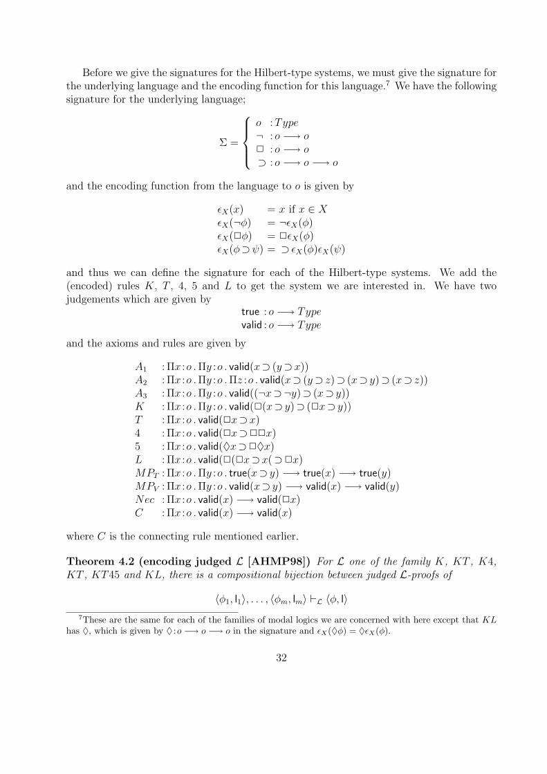
Before we give the signatures for the Hilbert-type systems, we must give the signature forthe underlying language and the encoding function for this language.7 We have the followingsignature for the underlying language;

Σ =

o :Type¬ : o −→ o2 : o −→ o⊃ : o −→ o −→ o

and the encoding function from the language to o is given by

εX(x) = x if x ∈ XεX(¬φ) = ¬εX(φ)εX(2φ) = 2εX(φ)εX(φ⊃ψ) = ⊃ εX(φ)εX(ψ)

and thus we can define the signature for each of the Hilbert-type systems. We add the(encoded) rules K, T , 4, 5 and L to get the system we are interested in. We have twojudgements which are given by

true : o −→ Typevalid : o −→ Type

and the axioms and rules are given by

A1 : Πx :o .Πy :o . valid(x⊃ (y⊃x))A2 : Πx :o .Πy :o .Πz :o . valid(x⊃ (y⊃ z)⊃ (x⊃ y)⊃ (x⊃ z))A3 : Πx :o .Πy :o . valid((¬x⊃¬y)⊃ (x⊃ y))K : Πx :o .Πy :o . valid(2(x⊃ y)⊃ (2x⊃ y))T : Πx :o . valid(2x⊃x)4 :Πx :o . valid(2x⊃22x)5 :Πx :o . valid(♦x⊃2♦x)L : Πx :o . valid(2(2x⊃x(⊃2x)MPT : Πx :o .Πy :o . true(x⊃ y) −→ true(x) −→ true(y)MPV : Πx :o .Πy :o . valid(x⊃ y) −→ valid(x) −→ valid(y)Nec : Πx :o . valid(x) −→ valid(2x)C : Πx :o . valid(x) −→ valid(x)

where C is the connecting rule mentioned earlier.

Theorem 4.2 (encoding judged L [AHMP98]) For L one of the family K, KT , K4,KT , KT45 and KL, there is a compositional bijection between judged L-proofs of

〈φ1, l1〉, . . . , 〈φm, lm〉 `L 〈φ, l〉7These are the same for each of the families of modal logics we are concerned with here except that KL

has ♦, which is given by ♦ :o −→ o −→ o in the signature and εX(♦φ) = ♦εX(φ).

32

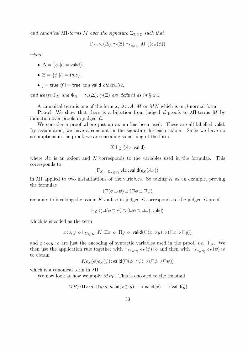
and canonical λΠ-terms M over the signature Σ2j(H) such that

ΓX , γv(∆), γt(Ξ) `Σ2j(L)M : j(εX(φ))

where

• ∆ = {φi|li = valid},

• Ξ = {φi|li = true},

• j = true if l = true and valid otherwise,

and where ΓX and ΦX = γv(∆), γt(Ξ) are defined as in § 2.3.

A canonical term is one of the form x, λx :A .M or MN which is in β-normal form.Proof We show that there is a bijection from judged L-proofs to λΠ-terms M by

induction over proofs in judged L.We consider a proof where just an axiom has been used. These are all labelled valid.

By assumption, we have a constant in the signature for each axiom. Since we have noassumptions in the proof, we are encoding something of the form

X `L 〈Ax, valid〉

where Ax is an axiom and X corresponds to the variables used in the formulae. Thiscorresponds to

ΓX `Σwj(H)Ax :valid(εX(Ax))

in λΠ applied to two instantiations of the variables. So taking K as an example, provingthe formulae

(2(φ⊃ψ)⊃ (2φ⊃2ψ)

amounts to invoking the axiom K and so in judged L corresponds to the judged L-proof

`L 〈(2(φ⊃ψ)⊃ (2φ⊃2ψ), valid〉

which is encoded as the term

x :o, y :o `Σ2j(H)K :Πx :o .Πy :o . valid(2(x⊃ y)⊃ (2x⊃2y))

and x : o, y : o are just the encoding of syntactic variables used in the proof, i.e. ΓX . Wethen use the application rule together with `Σ2j(H)

εX(φ) : o and then with `Σ2j(H)εX(ψ) : o

to obtainKεX(φ)εX(ψ) :valid(2(φ⊃ψ)⊃ (2φ⊃2ψ))

which is a canonical term in λΠ.We now look at how we apply MPV . This is encoded to the constant

MPV :Πx :o .Πy :o . valid(x⊃ y) −→ valid(x) −→ valid(y)

33

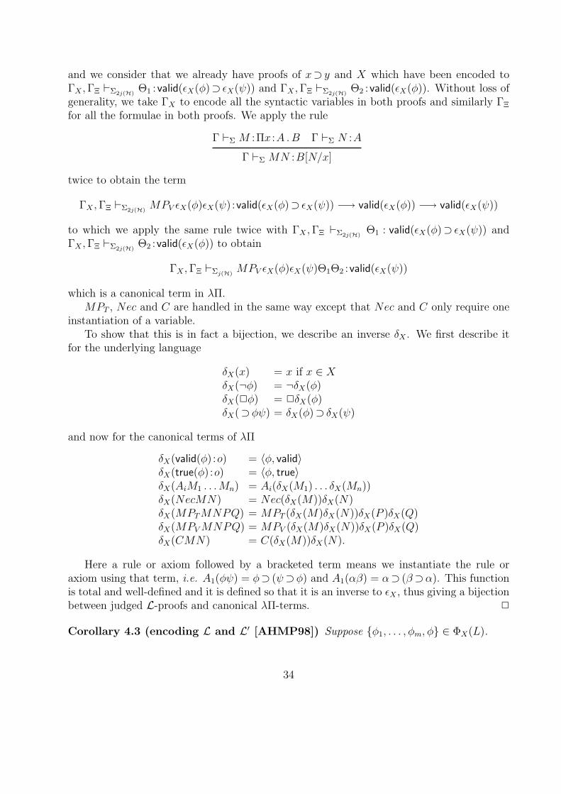
and we consider that we already have proofs of x⊃ y and X which have been encoded toΓX ,ΓΞ `Σ2j(H)

Θ1 :valid(εX(φ)⊃ εX(ψ)) and ΓX ,ΓΞ `Σ2j(H)Θ2 :valid(εX(φ)). Without loss of

generality, we take ΓX to encode all the syntactic variables in both proofs and similarly ΓΞ

for all the formulae in both proofs. We apply the rule

Γ `Σ M :Πx :A .B Γ `Σ N :A

Γ `Σ MN :B[N/x]

twice to obtain the term

ΓX ,ΓΞ `Σ2j(H)MPV εX(φ)εX(ψ) :valid(εX(φ)⊃ εX(ψ)) −→ valid(εX(φ)) −→ valid(εX(ψ))

to which we apply the same rule twice with ΓX ,ΓΞ `Σ2j(H)Θ1 : valid(εX(φ)⊃ εX(ψ)) and

ΓX ,ΓΞ `Σ2j(H)Θ2 :valid(εX(φ)) to obtain

ΓX ,ΓΞ `Σj(H)MPV εX(φ)εX(ψ)Θ1Θ2 :valid(εX(ψ))

which is a canonical term in λΠ.MPT , Nec and C are handled in the same way except that Nec and C only require one

instantiation of a variable.To show that this is in fact a bijection, we describe an inverse δX . We first describe it

for the underlying language

δX(x) = x if x ∈ XδX(¬φ) = ¬δX(φ)δX(2φ) = 2δX(φ)δX(⊃φψ) = δX(φ)⊃ δX(ψ)

and now for the canonical terms of λΠ

δX(valid(φ) :o) = 〈φ, valid〉δX(true(φ) :o) = 〈φ, true〉δX(AiM1 . . .Mn) = Ai(δX(M1) . . . δX(Mn))δX(NecMN) = Nec(δX(M))δX(N)δX(MPTMNPQ) = MPT (δX(M)δX(N))δX(P )δX(Q)δX(MPVMNPQ) = MPV (δX(M)δX(N))δX(P )δX(Q)δX(CMN) = C(δX(M))δX(N).

Here a rule or axiom followed by a bracketed term means we instantiate the rule oraxiom using that term, i.e. A1(φψ) = φ⊃ (ψ⊃φ) and A1(αβ) = α⊃ (β⊃α). This functionis total and well-defined and it is defined so that it is an inverse to εX , thus giving a bijectionbetween judged L-proofs and canonical λΠ-terms. 2

Corollary 4.3 (encoding L and L′ [AHMP98]) Suppose {φ1, . . . , φm, φ} ∈ ΦX(L).

34

1. There is a compositional bijection between proofs in L′ of φ1, . . . , φm ` φ and canonicalλΠ-terms M such that

ΓX , γv({φ1, . . . , φm}) `Σ2j(H)M :valid(εX(φ)).

2. There is a compositional bijection between proofs in L of φ1, . . . , φm ` φ and canonicalλΠ-terms M such that

ΓX , γt({φ1, . . . , φm}) `Σ2j(H)M : j(εX(φ)),

where j is valid, if either m = 0 or no φi occurs in the proof, and is true, otherwise.

Proof Any canonical λΠ-terms where the final type is of the form valid(εX(φ)) meansthat it corresponds to a proof in L′ since any λΠ-term which has it’s final node as valid musthave all successors as valid and by Lemma 4.1 there is a bijection.

If j = true then all of it’s successors must be valid and so it corresponds to a proof in Lby Lemma 4.1. If j = valid and m = 0 or no φi occurs in the proof, then no assumptionshave been used and so it corresponds to a proof in L. 2

Before embarking upon our technical development of judged logics, it will be useful toconsider a range of examples of normative formulations of object-logics and the representationmechanisms that can be used to encode them in LF, judgements-as-types being our leadingexample.

We identify three typical, though not exhaustive, cases. Again, we draw substantiallyupon [AHMP98] for background.

1. Proof-trees labelled with multiple judgements, encoded using the judgements-as-typesrepresentation mechanism. For examples:

• Hilbert-type formulations, for both truth and validity, of the modal systems, suchas K, K4, KT , S4, etc. discussed above. Two logical judgements, true and valid,are used.

• Natural deduction formulations, for validity, of the modal logics discussed above.Two logical judgements, true and valid are used.

• Natural deduction formulations, for truth and validity, of the modal logics dis-cussed above. Three logical judgements, taut, valid and true are used.

2. Proof-trees labelled (degenerately) with a single logical judgement, encoded using theworlds-as-parameters representation mechanism. For example:

• Hilbert-type formulations, for truth, of K, K4, KT , S4, etc.. In a worlds-as-parameters encoding, worlds are introduced via a sort, the “universe” which,having no constructors, is inhabited only by variables, or “worlds”. The useof these parameters is purely syntactic. They permit the representation of theglobal side-conditions found in the rules of proof, such as “no assumptions”, bytransferring them to metalogical conditions such as “no free variables”. Thedetails can be found in [AHMP98].

35

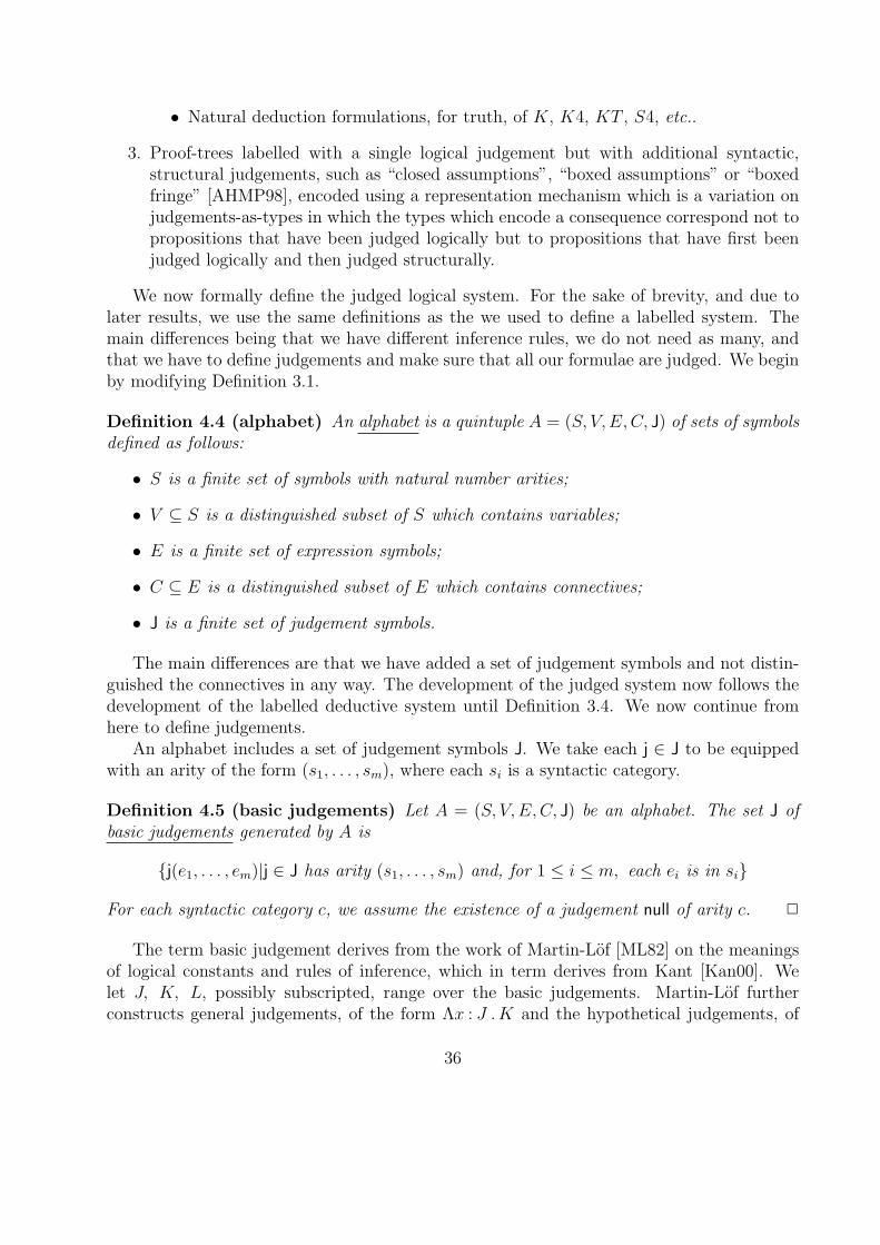
• Natural deduction formulations, for truth, of K, K4, KT , S4, etc..

3. Proof-trees labelled with a single logical judgement but with additional syntactic,structural judgements, such as “closed assumptions”, “boxed assumptions” or “boxedfringe” [AHMP98], encoded using a representation mechanism which is a variation onjudgements-as-types in which the types which encode a consequence correspond not topropositions that have been judged logically but to propositions that have first beenjudged logically and then judged structurally.

We now formally define the judged logical system. For the sake of brevity, and due tolater results, we use the same definitions as the we used to define a labelled system. Themain differences being that we have different inference rules, we do not need as many, andthat we have to define judgements and make sure that all our formulae are judged. We beginby modifying Definition 3.1.

Definition 4.4 (alphabet) An alphabet is a quintuple A = (S, V, E,C, J) of sets of symbolsdefined as follows:

• S is a finite set of symbols with natural number arities;

• V ⊆ S is a distinguished subset of S which contains variables;

• E is a finite set of expression symbols;

• C ⊆ E is a distinguished subset of E which contains connectives;

• J is a finite set of judgement symbols.

The main differences are that we have added a set of judgement symbols and not distin-guished the connectives in any way. The development of the judged system now follows thedevelopment of the labelled deductive system until Definition 3.4. We now continue fromhere to define judgements.

An alphabet includes a set of judgement symbols J. We take each j ∈ J to be equippedwith an arity of the form (s1, . . . , sm), where each si is a syntactic category.

Definition 4.5 (basic judgements) Let A = (S, V, E,C, J) be an alphabet. The set J ofbasic judgements generated by A is

{j(e1, . . . , em)|j ∈ J has arity (s1, . . . , sm) and, for 1 ≤ i ≤ m, each ei is in si}

For each syntactic category c, we assume the existence of a judgement null of arity c. 2

The term basic judgement derives from the work of Martin-Lof [ML82] on the meaningsof logical constants and rules of inference, which in term derives from Kant [Kan00]. Welet J, K, L, possibly subscripted, range over the basic judgements. Martin-Lof furtherconstructs general judgements, of the form Λx : J .K and the hypothetical judgements, of

36

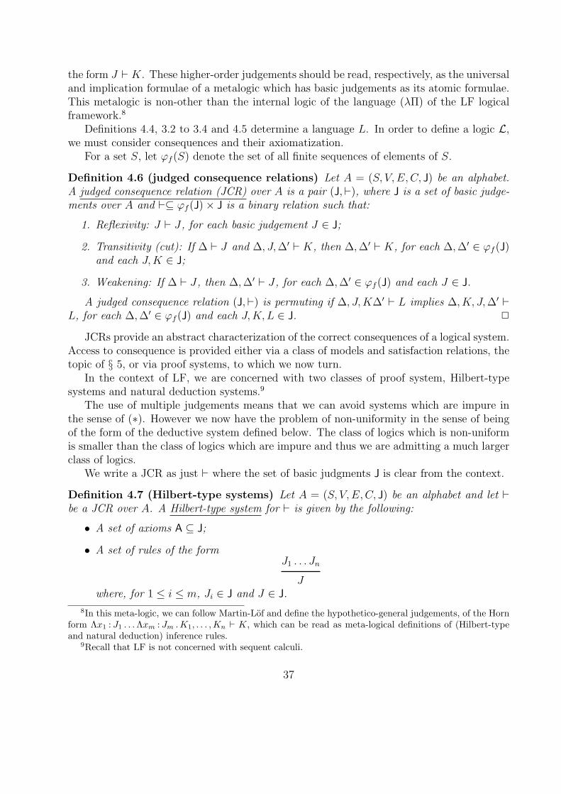
the form J ` K. These higher-order judgements should be read, respectively, as the universaland implication formulae of a metalogic which has basic judgements as its atomic formulae.This metalogic is non-other than the internal logic of the language (λΠ) of the LF logicalframework.8

Definitions 4.4, 3.2 to 3.4 and 4.5 determine a language L. In order to define a logic L,we must consider consequences and their axiomatization.

For a set S, let ϕf (S) denote the set of all finite sequences of elements of S.

Definition 4.6 (judged consequence relations) Let A = (S, V, E,C, J) be an alphabet.A judged consequence relation (JCR) over A is a pair (J,`), where J is a set of basic judge-ments over A and `⊆ ϕf (J)× J is a binary relation such that:

1. Reflexivity: J ` J , for each basic judgement J ∈ J;

2. Transitivity (cut): If ∆ ` J and ∆, J,∆′ ` K, then ∆,∆′ ` K, for each ∆,∆′ ∈ ϕf (J)and each J,K ∈ J;

3. Weakening: If ∆ ` J , then ∆,∆′ ` J , for each ∆,∆′ ∈ ϕf (J) and each J ∈ J.

A judged consequence relation (J,`) is permuting if ∆, J,K∆′ ` L implies ∆, K, J,∆′ `L, for each ∆,∆′ ∈ ϕf (J) and each J,K, L ∈ J. 2

JCRs provide an abstract characterization of the correct consequences of a logical system.Access to consequence is provided either via a class of models and satisfaction relations, thetopic of § 5, or via proof systems, to which we now turn.

In the context of LF, we are concerned with two classes of proof system, Hilbert-typesystems and natural deduction systems.9

The use of multiple judgements means that we can avoid systems which are impure inthe sense of (∗). However we now have the problem of non-uniformity in the sense of beingof the form of the deductive system defined below. The class of logics which is non-uniformis smaller than the class of logics which are impure and thus we are admitting a much largerclass of logics.

We write a JCR as just ` where the set of basic judgments J is clear from the context.

Definition 4.7 (Hilbert-type systems) Let A = (S, V, E,C, J) be an alphabet and let `be a JCR over A. A Hilbert-type system for ` is given by the following:

• A set of axioms A ⊆ J;

• A set of rules of the formJ1 . . . Jn

Jwhere, for 1 ≤ i ≤ m, Ji ∈ J and J ∈ J.

8In this meta-logic, we can follow Martin-Lof and define the hypothetico-general judgements, of the Hornform Λx1 : J1 . . .Λxm : Jm .K1, . . . ,Kn ` K, which can be read as meta-logical definitions of (Hilbert-typeand natural deduction) inference rules.

9Recall that LF is not concerned with sequent calculi.

37

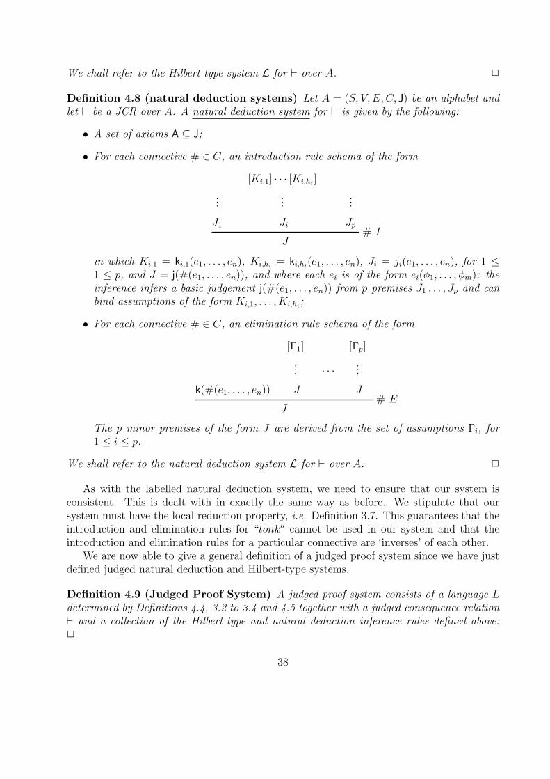
We shall refer to the Hilbert-type system L for ` over A. 2

Definition 4.8 (natural deduction systems) Let A = (S, V, E,C, J) be an alphabet andlet ` be a JCR over A. A natural deduction system for ` is given by the following:

• A set of axioms A ⊆ J;

• For each connective # ∈ C, an introduction rule schema of the form

...

J1

[Ki,1] · · · [Ki,hi]

...

Ji

...

Jp# I

J

in which Ki,1 = ki,1(e1, . . . , en), Ki,hi= ki,hi

(e1, . . . , en), Ji = ji(e1, . . . , en), for 1 ≤1 ≤ p, and J = j(#(e1, . . . , en)), and where each ei is of the form ei(φ1, . . . , φm): theinference infers a basic judgement j(#(e1, . . . , en)) from p premises J1 . . . , Jp and canbind assumptions of the form Ki,1, . . . , Ki,hi

;

• For each connective # ∈ C, an elimination rule schema of the form

k(#(e1, . . . , en))

[Γ1]

...

J

· · ·

[Γp]

...

J# E

J

The p minor premises of the form J are derived from the set of assumptions Γi, for1 ≤ i ≤ p.

We shall refer to the natural deduction system L for ` over A. 2

As with the labelled natural deduction system, we need to ensure that our system isconsistent. This is dealt with in exactly the same way as before. We stipulate that oursystem must have the local reduction property, i.e. Definition 3.7. This guarantees that theintroduction and elimination rules for “tonk′′ cannot be used in our system and that theintroduction and elimination rules for a particular connective are ‘inverses’ of each other.

We are now able to give a general definition of a judged proof system since we have justdefined judged natural deduction and Hilbert-type systems.

Definition 4.9 (Judged Proof System) A judged proof system consists of a language Ldetermined by Definitions 4.4, 3.2 to 3.4 and 4.5 together with a judged consequence relation` and a collection of the Hilbert-type and natural deduction inference rules defined above.2

38

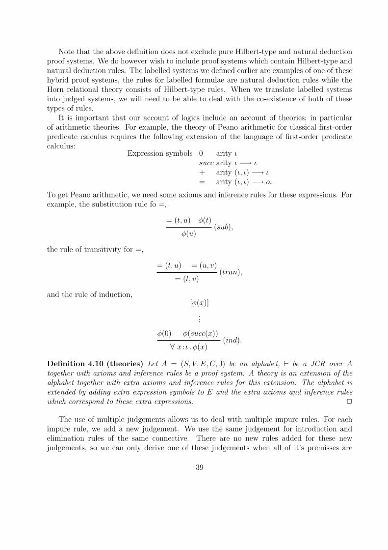
Note that the above definition does not exclude pure Hilbert-type and natural deductionproof systems. We do however wish to include proof systems which contain Hilbert-type andnatural deduction rules. The labelled systems we defined earlier are examples of one of thesehybrid proof systems, the rules for labelled formulae are natural deduction rules while theHorn relational theory consists of Hilbert-type rules. When we translate labelled systemsinto judged systems, we will need to be able to deal with the co-existence of both of thesetypes of rules.

It is important that our account of logics include an account of theories; in particularof arithmetic theories. For example, the theory of Peano arithmetic for classical first-orderpredicate calculus requires the following extension of the language of first-order predicatecalculus:

Expression symbols 0 arity ιsucc arity ι −→ ι+ arity (ι, ι) −→ ι= arity (ι, ι) −→ o.

To get Peano arithmetic, we need some axioms and inference rules for these expressions. Forexample, the substitution rule fo =,

= (t, u) φ(t)(sub),

φ(u)

the rule of transitivity for =,

= (t, u) = (u, v)(tran),

= (t, v)

and the rule of induction,

φ(0)

[φ(x)]

...

φ(succ(x))(ind).

∀ x : ι . φ(x)

Definition 4.10 (theories) Let A = (S, V, E,C, J) be an alphabet, ` be a JCR over Atogether with axioms and inference rules be a proof system. A theory is an extension of thealphabet together with extra axioms and inference rules for this extension. The alphabet isextended by adding extra expression symbols to E and the extra axioms and inference ruleswhich correspond to these extra expressions. 2

The use of multiple judgements allows us to deal with multiple impure rules. For eachimpure rule, we add a new judgement. We use the same judgement for introduction andelimination rules of the same connective. There are no new rules added for these newjudgements, so we can only derive one of these judgements when all of it’s premisses are

39

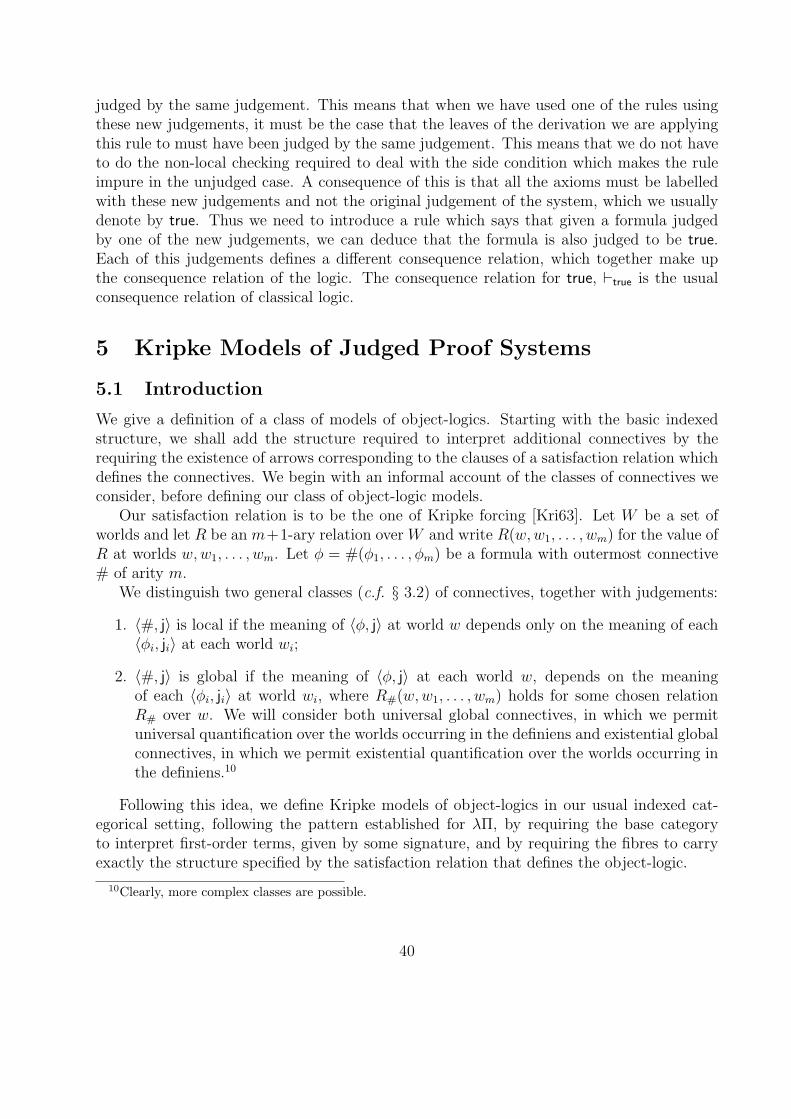
judged by the same judgement. This means that when we have used one of the rules usingthese new judgements, it must be the case that the leaves of the derivation we are applyingthis rule to must have been judged by the same judgement. This means that we do not haveto do the non-local checking required to deal with the side condition which makes the ruleimpure in the unjudged case. A consequence of this is that all the axioms must be labelledwith these new judgements and not the original judgement of the system, which we usuallydenote by true. Thus we need to introduce a rule which says that given a formula judgedby one of the new judgements, we can deduce that the formula is also judged to be true.Each of this judgements defines a different consequence relation, which together make upthe consequence relation of the logic. The consequence relation for true, `true is the usualconsequence relation of classical logic.

5 Kripke Models of Judged Proof Systems

5.1 Introduction

We give a definition of a class of models of object-logics. Starting with the basic indexedstructure, we shall add the structure required to interpret additional connectives by therequiring the existence of arrows corresponding to the clauses of a satisfaction relation whichdefines the connectives. We begin with an informal account of the classes of connectives weconsider, before defining our class of object-logic models.

Our satisfaction relation is to be the one of Kripke forcing [Kri63]. Let W be a set ofworlds and let R be an m+1-ary relation over W and write R(w,w1, . . . , wm) for the value ofR at worlds w,w1, . . . , wm. Let φ = #(φ1, . . . , φm) be a formula with outermost connective# of arity m.

We distinguish two general classes (c.f. § 3.2) of connectives, together with judgements:

1. 〈#, j〉 is local if the meaning of 〈φ, j〉 at world w depends only on the meaning of each〈φi, ji〉 at each world wi;

2. 〈#, j〉 is global if the meaning of 〈φ, j〉 at each world w, depends on the meaningof each 〈φi, ji〉 at world wi, where R#(w,w1, . . . , wm) holds for some chosen relationR# over w. We will consider both universal global connectives, in which we permituniversal quantification over the worlds occurring in the definiens and existential globalconnectives, in which we permit existential quantification over the worlds occurring inthe definiens.10

Following this idea, we define Kripke models of object-logics in our usual indexed cat-egorical setting, following the pattern established for λΠ, by requiring the base categoryto interpret first-order terms, given by some signature, and by requiring the fibres to carryexactly the structure specified by the satisfaction relation that defines the object-logic.

10Clearly, more complex classes are possible.

40

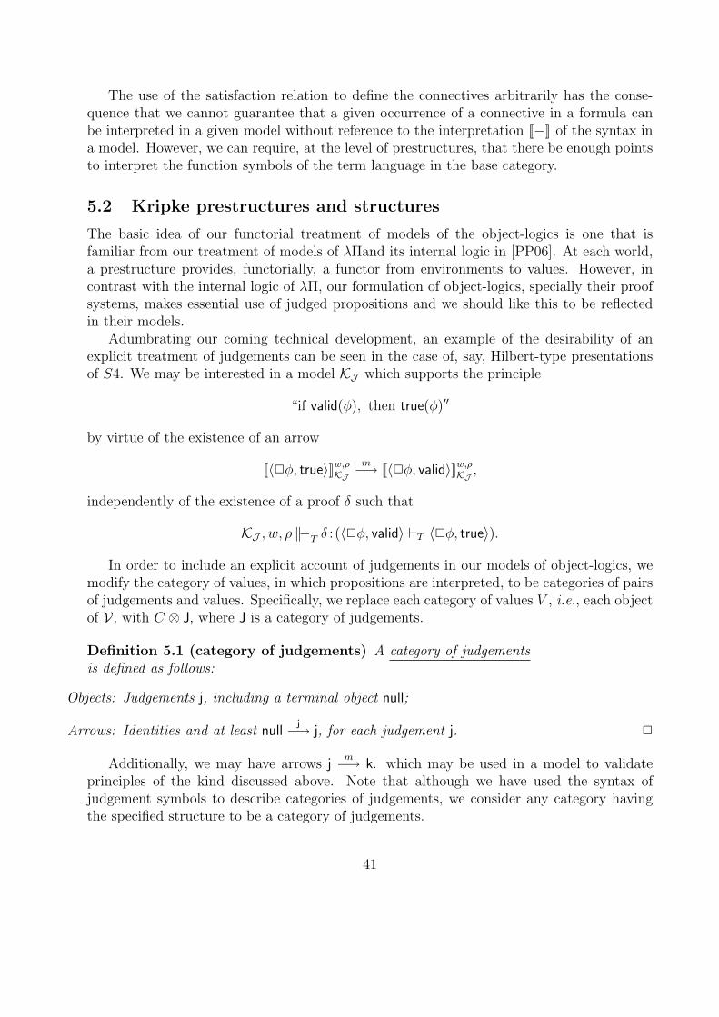
The use of the satisfaction relation to define the connectives arbitrarily has the conse-quence that we cannot guarantee that a given occurrence of a connective in a formula canbe interpreted in a given model without reference to the interpretation [[−]] of the syntax ina model. However, we can require, at the level of prestructures, that there be enough pointsto interpret the function symbols of the term language in the base category.

5.2 Kripke prestructures and structures

The basic idea of our functorial treatment of models of the object-logics is one that isfamiliar from our treatment of models of λΠand its internal logic in [PP06]. At each world,a prestructure provides, functorially, a functor from environments to values. However, incontrast with the internal logic of λΠ, our formulation of object-logics, specially their proofsystems, makes essential use of judged propositions and we should like this to be reflectedin their models.

Adumbrating our coming technical development, an example of the desirability of anexplicit treatment of judgements can be seen in the case of, say, Hilbert-type presentationsof S4. We may be interested in a model KJ which supports the principle

“if valid(φ), then true(φ)′′

by virtue of the existence of an arrow

[[〈2φ, true〉]]w,ρKJ

m−→ [[〈2φ, valid〉]]w,ρKJ ,

independently of the existence of a proof δ such that

KJ , w, ρ ‖−T δ : (〈2φ, valid〉 `T 〈2φ, true〉).

In order to include an explicit account of judgements in our models of object-logics, wemodify the category of values, in which propositions are interpreted, to be categories of pairsof judgements and values. Specifically, we replace each category of values V , i.e., each objectof V , with C ⊗ J, where J is a category of judgements.

Definition 5.1 (category of judgements) A category of judgementsis defined as follows:

Objects: Judgements j, including a terminal object null;

Arrows: Identities and at least nullj−→ j, for each judgement j. 2

Additionally, we may have arrows jm−→ k. which may be used in a model to validate

principles of the kind discussed above. Note that although we have used the syntax ofjudgement symbols to describe categories of judgements, we consider any category havingthe specified structure to be a category of judgements.

41

A judged proposition 〈φ, j〉 is interpreted in a category of judged values formed by forminga product (in C) of a category of judgements and a category of values. The transition inthe semantics from values to judged values is directly, and deliberately, analogous to thetransition from proof trees to proof trees labelled with judgements, which is characterizedusing the techniques of Lemma 4.1.

Definition 5.2 (judged values) A category of judged values is a category

V ⊗ J

where J is a category of judgements, V is a category (of values) and ⊗ is the product in C.2

We are always able to construct the category of judged values because both V and Jlive in the category of small categories and functors which is cartesian closed. Thus there isalways a product operation defined in this category which we are able to apply to V and J.

For example, in our judged view of intuitionistic propositional logic, we have just onejudgement, proof. In this case, the category of judgements J is exactly

-proof

·�null

·1proof

and a judged proposition 〈φ, proof〉 is interpreted as an object [[φ]]w,ρKJ ⊗ proof of V ⊗ J. A

proof δ of 〈φ, proof〉, from judged assumptions Γ, is interpreted as an arrow

1⊗ null[[δ]]w,ρ

KJ⊗proof

−→ [[φ]]w,ρKJ ⊗ proof,

where δ denotes the corresponding unjudged proof tree, which can be characterized usingthe techniques of Lemma 4.1.

When we interpret a logic in a category, we need to make sure that the category hasenough structure to interpret each constant of the language and keeps each constant of thesame sort distinct. We define this condition:

Definition 5.3 (enough points) We say that a category C has enough points to interpret

a language L if for each constant c :S, there exists an arrow 1c−→ [[S]] and for two constants

c1 :S 6= c2 :S, interpreted 1c1−→ [[S]] and 1

c2−→ [[S]], we have that for all arrows f : [[S]] −→ [[S ′]]that fc1 6= fc2. 2

42

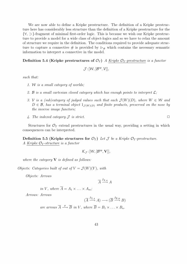
We are now able to define a Kripke prestructure. The definition of a Kripke prestruc-ture here has considerably less structure than the definition of a Kripke prestructure for the{∀, ⊃}-fragment of minimal first-order logic. This is because we wish our Kripke prestruc-ture to provide a model for a wide class of object-logics and so we have to relax the amountof structure we require in the definition. The conditions required to provide adequate struc-ture to capture a connective # is provided by �# which contains the necessary semanticinformation to interpret a connective in the model.

Definition 5.4 (Kripke prestructures of OT ) A Kripke OT -prestructure is a functor

J : [W , [Bop,V ]],

such that:

1. W is a small category of worlds;

2. B is a small cartesian closed category which has enough points to interpret L;

3. V is a (sub)category of judged values such that each J (W )(D), where W ∈ W andD ∈ B, has a terminal object 1J (W )(D) and finite products, preserved on the nose bythe inverse image functors;

4. The indexed category J is strict. 2

Structures for OT extend prestructures in the usual way, providing a setting in whichconsequences can be interpreted.

Definition 5.5 (Kripke structures for OT ) Let J be a Kripke OT -prestructure.A Kripke OT -structure is a functor

KJ : [W , [Bop,V]],

where the category V is defined as follows:

Objects: Categories built of out of V = J (W )(Y ), with

Objects: Arrows

AfA,A−→ A

in V , where A = A1 × . . .× Am;

Arrows: Arrows

(AfA,A−→ A) −→ (B

fB,B−→ B)

are arrows Aµ−→ B in V , where B = B1 × . . .×Bn.

43

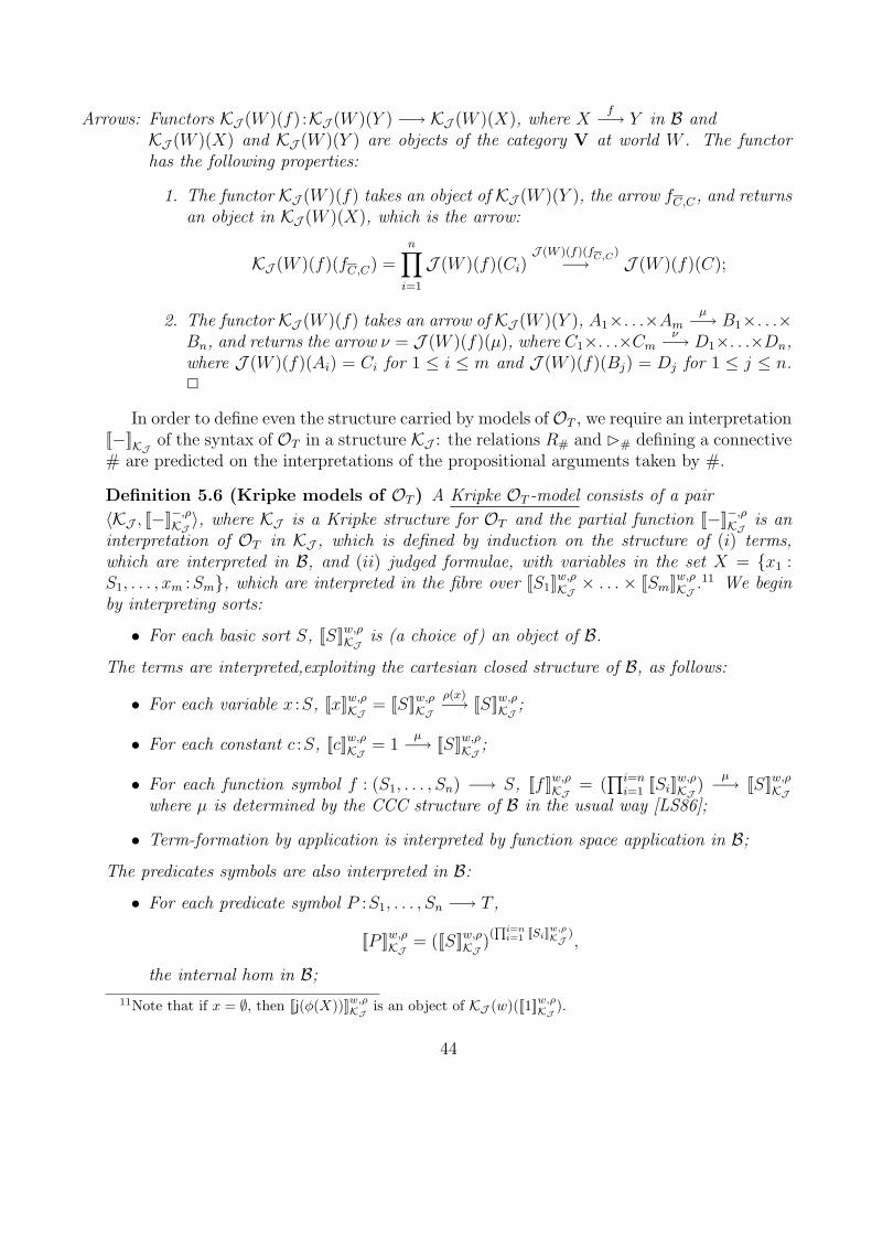
Arrows: Functors KJ (W )(f) :KJ (W )(Y ) −→ KJ (W )(X), where Xf−→ Y in B and

KJ (W )(X) and KJ (W )(Y ) are objects of the category V at world W . The functorhas the following properties:

1. The functor KJ (W )(f) takes an object of KJ (W )(Y ), the arrow fC,C, and returnsan object in KJ (W )(X), which is the arrow:

KJ (W )(f)(fC,C) =n∏

i=1

J (W )(f)(Ci)J (W )(f)(fC,C)−→ J (W )(f)(C);

2. The functor KJ (W )(f) takes an arrow of KJ (W )(Y ), A1×. . .×Amµ−→ B1×. . .×

Bn, and returns the arrow ν = J (W )(f)(µ), where C1×. . .×Cmν−→ D1×. . .×Dn,

where J (W )(f)(Ai) = Ci for 1 ≤ i ≤ m and J (W )(f)(Bj) = Dj for 1 ≤ j ≤ n.2

In order to define even the structure carried by models of OT , we require an interpretation[[−]]KJ of the syntax of OT in a structure KJ : the relations R# and �# defining a connective# are predicted on the interpretations of the propositional arguments taken by #.

Definition 5.6 (Kripke models of OT ) A Kripke OT -model consists of a pair

〈KJ , [[−]]−,ρKJ 〉, where KJ is a Kripke structure for OT and the partial function [[−]]−,ρ

KJ is aninterpretation of OT in KJ , which is defined by induction on the structure of (i) terms,which are interpreted in B, and (ii) judged formulae, with variables in the set X = {x1 :S1, . . . , xm :Sm}, which are interpreted in the fibre over [[S1]]

w,ρKJ × . . . × [[Sm]]w,ρ

KJ .11 We beginby interpreting sorts:

• For each basic sort S, [[S]]w,ρKJ is (a choice of) an object of B.

The terms are interpreted,exploiting the cartesian closed structure of B, as follows:

• For each variable x :S, [[x]]w,ρKJ = [[S]]w,ρ

KJρ(x)−→ [[S]]w,ρ

KJ ;

• For each constant c :S, [[c]]w,ρKJ = 1

µ−→ [[S]]w,ρKJ ;

• For each function symbol f : (S1, . . . , Sn) −→ S, [[f ]]w,ρKJ = (

∏i=ni=1 [[Si]]

w,ρKJ )

µ−→ [[S]]w,ρKJ

where µ is determined by the CCC structure of B in the usual way [LS86];

• Term-formation by application is interpreted by function space application in B;

The predicates symbols are also interpreted in B:

• For each predicate symbol P :S1, . . . , Sn −→ T ,

[[P ]]w,ρKJ = ([[S]]w,ρ

KJ )(Qi=n

i=1 [[Si]]w,ρKJ

),

the internal hom in B;11Note that if x = ∅, then [[j(φ(X))]]w,ρ

KJ is an object of KJ (w)([[1]]w,ρKJ ).

44

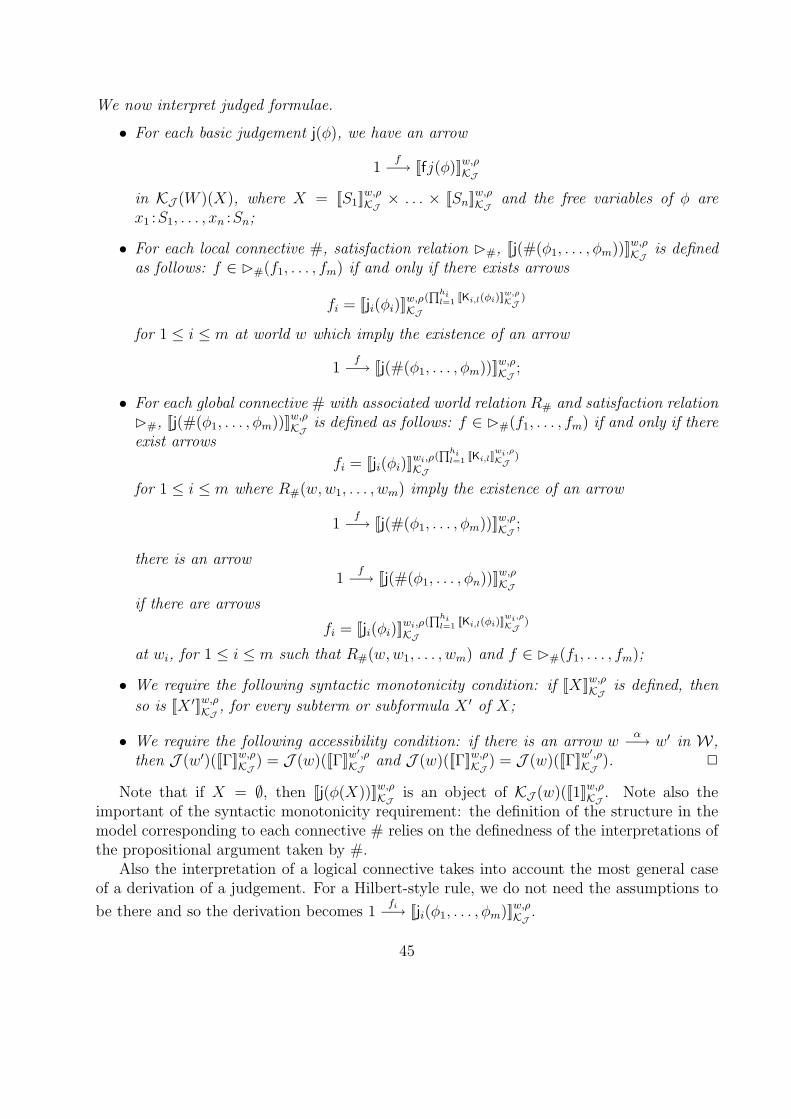
We now interpret judged formulae.

• For each basic judgement j(φ), we have an arrow

1f−→ [[fj(φ)]]w,ρ

KJ

in KJ (W )(X), where X = [[S1]]w,ρKJ × . . . × [[Sn]]w,ρ

KJ and the free variables of φ arex1 :S1, . . . , xn :Sn;

• For each local connective #, satisfaction relation �#, [[j(#(φ1, . . . , φm))]]w,ρKJ is defined

as follows: f ∈ �#(f1, . . . , fm) if and only if there exists arrows

fi = [[ji(φi)]]w,ρKJ

(Qhi

l=1 [[Ki,l(φi)]]w,ρKJ

)

for 1 ≤ i ≤ m at world w which imply the existence of an arrow

1f−→ [[j(#(φ1, . . . , φm))]]w,ρ

KJ ;

• For each global connective # with associated world relation R# and satisfaction relation�#, [[j(#(φ1, . . . , φm))]]w,ρ

KJ is defined as follows: f ∈ �#(f1, . . . , fm) if and only if thereexist arrows

fi = [[ji(φi)]]wi,ρKJ

(Qhi

l=1 [[Ki,l]]wi,ρKJ

)

for 1 ≤ i ≤ m where R#(w,w1, . . . , wm) imply the existence of an arrow

1f−→ [[j(#(φ1, . . . , φm))]]w,ρ

KJ ;

there is an arrow1

f−→ [[j(#(φ1, . . . , φn))]]w,ρKJ

if there are arrows

fi = [[ji(φi)]]wi,ρKJ

(Qhi

l=1 [[Ki,l(φi)]]wi,ρKJ

)

at wi, for 1 ≤ i ≤ m such that R#(w,w1, . . . , wm) and f ∈ �#(f1, . . . , fm);

• We require the following syntactic monotonicity condition: if [[X]]w,ρKJ is defined, then

so is [[X ′]]w,ρKJ , for every subterm or subformula X ′ of X;

• We require the following accessibility condition: if there is an arrow wα−→ w′ in W,

then J (w′)([[Γ]]w,ρKJ ) = J (w)([[Γ]]w

′,ρKJ and J (w)([[Γ]]w,ρ

KJ ) = J (w)([[Γ]]w′,ρ

KJ ). 2

Note that if X = ∅, then [[j(φ(X))]]w,ρKJ is an object of KJ (w)([[1]]w,ρ

KJ . Note also theimportant of the syntactic monotonicity requirement: the definition of the structure in themodel corresponding to each connective # relies on the definedness of the interpretations ofthe propositional argument taken by #.

Also the interpretation of a logical connective takes into account the most general caseof a derivation of a judgement. For a Hilbert-style rule, we do not need the assumptions to

be there and so the derivation becomes 1fi−→ [[ji(φ1, . . . , φm)]]w,ρ

KJ .

45

5.3 Soundness and Completeness of Kripke Models

We can now complete our semantic view of object-logics by defining the satisfaction of aproposition in a model. The satisfaction relations �# are part of the semantic definitions ofthe connectives #. Here we are concerned with the satisfaction relation for the whole logic.

Definition 5.7 (satisfaction) Let KJ be a Kripke OT -model. KJ satisfies j(φ) at world wwith respect to environment ρ,

w, ρ ‖−T j(φ)

if and only if there is an arrow

1f−→ [[j(φ)]]w,ρ

KJ .

If Γ = j1(φ1), . . . , jm(φm), then we write w, ρ ‖−T Γ if, for each 1 ≤ i ≤ m, w, ρ ‖−T ji(φi).We write w, ρ ‖−T (Γ `OT

j(φ) or more commonly w, ρΓ ‖−T j(φ), if w, ρ ‖−T Γimplies w, ρ ‖−T j(φ). 2

We prove a result about monotonicity of satisfaction.

Lemma 5.8 (monotonicity of satisfaction) Let OT be an object-logic and 〈KJ , [[−]]−,ρKJ 〉

be a Kripke OT -model. If w, ρ ‖−T j(φ), wα−→ w′ then w′, ρ ‖−T j(φ).

Proof By the accessibility condition of Definition 5.6, wα−→ w′ gives us the existence

of an arrow 1f ′−→ [[j(φ)]]w

′,ρKJ and thus w′, ρ ‖−T j(φ). 2

We refer the reader to the work of Aczel [Acz80], where he presents a logical systemwhich is very similar in style to the one presented in Definitions 4.4,3.2 to 3.4 and 4.5 exceptthat it is less general. He only has one judgement true and does not treat logical connectivesin general. In fact, his definition of a Frege structure can be considered as a logic accordingto our definition, since we can just add the extra the extra logical connectives λ and appto classical logic. The idea of not being able to define truth internally within a languageand the split between the logic and the metalogic can be captured more explicitly in thesetup we are using. This link between the work of Aczel and our own is expressed by thecomment in the final section that the type theory of Martin-Lof, which we are using here canbe modeled in a suitably chosen Frege structure and we are providing the opposite view thatFrege structures can be expressed in Martin-Lof type theory. The lambda structure of Aczelcan be seen to correspond to the λΠ-calculus that we use as a metalogic. The definition ofan iterative set, the smallest collection of objects χ such that every set of χ’s is in χ can alsobe carried over into our setting to allow us to have a concept of an iterative set.

We prove a general soundness and completeness result for a judged proof system. We willreturn to these results later on and consider when they hold for specific classes of object-logicsand so obtain some representation results.

Lemma 5.9 (soundness of OT for ‖−T ) Let 〈KJ , [[−]]−,ρKJ 〉 be a Kripke OT -model and let

w be any world in this model. If Γ `OTj(φ), then w, ρ,Γ ‖−T j(φ).

46

Proof The proof proceeds by induction over the structure of proofs in the object-logic.We begin with the case where we have an axiom. Here we have j(φ) ∈ Γ and so by

induction hypothesis, we have an arrow 1f−→ [[j(φ)]]w,ρ

KJ .We now look at an introduction rule. We have that w, ρ,Γ′ ‖−T ji(φi) for 1 ≤ i ≤ n,

where Γ′ is Γ plus any hypotheses. By the induction hypothesis, we have arrows

[[ji(φi)]]w,ρKJ

(Qhi

l=1 [[Ki,l(φi)]]w,ρKJ

)for each 1 ≤ i ≤ n. By Definition 5.6, we have that there exists an

arrow 1f−→ [[j(#(φ1, . . . , φn))]]w,ρ

KJ with f ∈ �#(f1, . . . , fn) and thusw, ρ,Γ ‖−T j(#(φ1, . . . , φn)).

Finally, we consider an elimination rule. We have that w, ρ,Γ ‖−T k(#(φ1, . . . , φn)) andw, ρ,Γ′ ‖−T j(φ), where Γ′ is Γ plus any hypotheses. By the induction hypothesis, we have

arrows 1f−→ [[k(#(φ1, . . . , φn))]]w,ρ

KJ and [[j(φ)]]w,ρKJ

([[Ki]]w,ρKJ

)for 1 ≤ i ≤ n. Since we are in a

Cartesian closed category, we obtain 1 −→ [[j(φ1, . . . , φn)]]w,ρKJ and thus w, ρ,Γ ‖−T j(φ). 2

To prove completeness, we construct a model where there exists a world w0 such thatΓ 6`T j(φ) implies w0, ρ,Γ 6 ‖−T j(φ). We begin by constructing a categorical structure whichwe will prove is a Kripke OT -structure and then give it an interpretation which gives theresult.

Going back to our motivation for constructing Kripke models, we recall that we wishto use Kripke partiality to determine which proof variables are defined at a world and thuswhich formulae have proofs. We take worlds to be collections of proof variables. Thus wehave a proof is true at a particular world if and only if it’s proof variable is at that world orall the proof variables in it’s assumptions hold at that world.

Informally, our term model has the following structure; a base category which capturesterms, here the objects are products of sorts and the arrows are realizations, and fibres overthe base category which will capture consequence. The objects of each fibre will be proofsand the arrows proof transformations.

We begin by defining the base category, B(A).

Definition 5.10 Let A be an alphabet. The (base) category B(A) of sorts and realizationsis defined as follows:

Objects: Products of sorts∏m

i=1 Si such that Si correspond to the syntactic categories of thelanguage generated by the alphabet;

Arrows: Realizations X〈t1,...,tn〉−→ Y such that x1 :S1, . . . , xm :Si `OT

ti :Ti for all 1 ≤ i ≤ n;

– Identities, written idX , are S1 × . . .× Sm〈x1,...,xm〉−→ S1 × . . .× Sm.

– Composition is defined as follows: if σ = X〈t1,...,tn〉−→ Y and ρ = Y

〈s1,...,sp〉−→ Z, then

σ; ρ = X〈s1[tj/yj ]

nj=1,...,sp[xj/yj ]

nj=1〉−→ Z. 2

Here variables are understood as a special case of the identity. A variable is just the

identity on a single sort, i.e. S〈x〉−→ S.

47

Before we define out Kripke prestructure, we define a strict indexed category over thebase category, which we will use to construct the Kripke prestructure.

Definition 5.11 We define inductively a strict indexed category E(A) over the base categorycalB(A),

E(A) :B(A)op −→ C,where C denotes the category of small categories and functors, as follows:

• For each product of sorts, S = S1 × . . .× Sn in B(A), the category E(A)(S) is definedas follows:

Objects: Judged formulae j(P (t1, . . . , tn)) such that x1 :S1, . . . , xn :Sn `OTj(P (t1, . . . , tn));

Arrows: j(P (t1, . . . , tn))t−→ j(Q(r1, . . . , rm)), where the arrow t is such that S1× . . .×Sn×

T〈x,t〉−→ S1× . . .×Sn×U in B(A), where j(P (t1, . . . , tn)) :T and j(W (r1, . . . , rp)) :U ;

if j(P (t1, . . . , tn))t−→ j(Q(r1, . . . , rm)) and j(Q(r1, . . . , rm))

u−→ j(R(u1, . . . , up)),

then j(P (t1, . . . , tn))t;u−→ j(R(u1, . . . , up)) is given by

j(P (t1, . . . , tn))u[t/U ]−→ j(R(u1, . . . , up)), where u is such that S1 × Sn × V

〈x,u〉−→ S1 ×. . .× Sn × U is an arrow in B(A);

• For each Yσ−→ X in B(A), E(A)(Y

σ−→ X) is a functor E(A)(X)σ∗−→ E(A)(Y )

given by σ∗j(P (t1, . . . , tn)) = j(P (t1, . . . , tn))[yi/xi]mi=1, where x1 : S1, . . . , xn : Sn and

y1 : T1, . . . , ym : Tm and σ∗j(P (t1, . . . , tn)) −→ j(Q(r1, . . . , rp) = σ∗j(P (t1, . . . , tn)) −→σ∗j(Q(r1, . . . , rp)). 2

Before we construct our Kripke prestructure, we have to define our category of worlds.To fully exploit the Kripke partiality of the model we are constructing, we take worlds tobe collections of proof variables, this will then tell us what we can and can not prove in thefibres over the base category.

Definition 5.12 We define a category of proof variables, W, as follows:

Objects: Sets of proof variables {ζ1, . . . , ζn};

Arrows: Given by subset inclusion. 2

For a proof j(φ) to be defined in a suitable fibre, we need to be over the world containingat least the proof variable ζ which corresponds to j(φ). This is the heart of our use of Kripkepartiality.

Over each world X, we place a base category B(A). We define a functorT (A) : [W , [B(A)op,V ], which will be our Kripke prestructure. Given an object S = S1 ×. . .× Sn of B(A), the functor T (A)(W ) gives us the following category:

T (A)(W )(S) =

Objects : Judged formulae j(φ) such that

x1 :S1, . . . , xn :Sn `OTj(φ) and ζ ∈ W ;

Arrows : E(A)(X) arrows;

48

where ζ is the proof variable corresponding to j(φ).From this, we build the Kripke structure, following the construction defined in Definition

5.5. This construction will give the term model. Need to fill in the details that

this thing is indeed a functor category.

The interpretation required to show that this is a Kripke OT -model is the obvious one, weinterpret the proof object (X) Γ `OT

j(φ) as an arrow 1 −→ [[j(φ)]]w,ρKJ in the fibre KJ (W )(T ),

where T = S1 × . . . × Sn and X = x1 :S1, . . . , xn :Sn and ζi ∈ W for each ζi correspondingto a proof of ji(φi) ∈ Γ.

From the definition of satisfaction, we have that Γ `OTj(φ) iff w, ρ,Γ ‖−T j(φ). If we take

w0 = ∅, then we have that Γ 6`OTj(φ) implies w0, ρ,Γ 6 ‖−T j(φ), thus we have the following

model existence result.

Lemma 5.13 (model existence) There exists a Kripke OT -model 〈KJ , [[−]]−,ρKJ 〉 with a

world w0 such that if there exists a proof δ : (Γ 6`OTj(φ)), then

w0, ρ,Γ 6 ‖−T j(φ).

Proof See the previous construction. 2

The term model we have constructed above has the correct property to allow us to provecompleteness

Theorem 5.14 (completeness) δ : ((X) Γ `OTj(φ)) if and only if w, ρ,Γ ‖−T j(φ).

Proof

(only if) This is soundness, Lemma 5.9.

(if) Suppose δ : ((X)Γ `OTj(φ)), then Lemma 5.13 yields a contradiction. 2

6 Judgements-as-types

6.1 Introduction

Having described a judged object-logic, we now describe how to encode this logic into a signa-ture in the λΠ-calculus and thus how it is represented in a logical framework. The encoding isthe judgements-as-types correspondence, this is a generalization of the propositions-as-typescorrespondence discussed in I and well known in the literature.

In particular, following Kant [Kan00] and Martin-Lof [ML82], we consider a metatheoryof object-logics in which the basic units manipulated by rules of inference are judged propo-sitions rather than the bare propositions. This is the judgements-as-types correspondence.

We describe how to take a proof-object δ : ((X)∆ `OTj(φ) and translate it to a λΠ-

term ΓX ,Γ∆ `ΣOTMδ : j(φ). We encode the inference rules of the object-logic as constants

in the signature of λΠ and then construct the term in λΠ. The rules of λΠ allow us tomimic applications of inference rules in the object-logic and so allow us to construct termscorresponding to proof-objects in the object-logic.

49

Once we have the encoding defined, we are able to talk about the properties of the mapfrom the syntax of the object-logic to the syntax of λΠ and it’s properties. In particular,we are able to define full and faithful encodings, as well as whether or not an encoding isuniform.

The judgements-as-types correspondence is not the only choice of representation mecha-nism, worlds-as-parameters is another paradigm we could have employed. The judgements-as-types correspondence has a more solid philosophical background and is a generalizationof the propositions-as-types correspondence which is the basis for the majority of proof the-oretic study. The use of a type of worlds which is not constructed seems to be less naturalthan the judgements-as-types correspondence.

We look at the judgements-as-types correspondence in two senses; the first is syntacticand provides us with an encoding mechanism, the second is semantic and provides us witha morphism of models. These two viewpoints are related in the following way: the encodingfunction will induce the morphism of models and properties of the encoding function willbe mirrored in the morphism of models. So a bijective encoding function will induce anisomorphism of models and a surjective encoding function will induce an epimorphism ofmodels. We begin by looking at the syntactic judgements-as-types before setting up the nec-essary categorical framework to describe the morphism and finally exploring the relationshipbetween the encoding and the induced morphism.

6.2 Syntactic judgements-as-types: Encoding logics in LF

We recall that an object-logic OT is an alphabet A = (S, V, E,C, J), made up of symbols,variable symbols, expressions, connectives and judgements and a collection of inference rules.We encode all of these as constants contained in the signature of λΠ. The idea behind theencoding of the an inference rule is the following; given a rule

...

j1(φ1) · · ·

...

jn(φn)

j(φ)

we think of it being quantified over all φ and each of the derivations of the judgements beinggiven by arrows and the combination of all the derivations being arrows, thus:

∏φ

...

j1(φ1)

∪⊃· · ·

...

jn(φn)

∪

∪j(φ)

With the∏

corresponding to Π in the λΠ-calculus and ⊃ corresponding to −→. Usually, theassumptions are understood as being joined by conjunction rather than implication, in thesense of if we have this assumption and this assumption . . ., then we have the conclusion.With a bit of thought, it can be seen that using implication here instead of conjunction

50

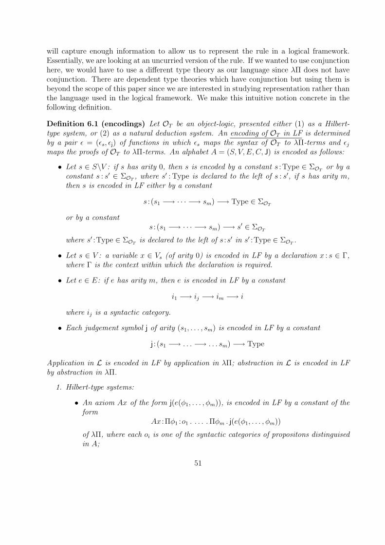
will capture enough information to allow us to represent the rule in a logical framework.Essentially, we are looking at an uncurried version of the rule. If we wanted to use conjunctionhere, we would have to use a different type theory as our language since λΠ does not haveconjunction. There are dependent type theories which have conjunction but using them isbeyond the scope of this paper since we are interested in studying representation rather thanthe language used in the logical framework. We make this intuitive notion concrete in thefollowing definition.

Definition 6.1 (encodings) Let OT be an object-logic, presented either (1) as a Hilbert-type system, or (2) as a natural deduction system. An encoding of OT in LF is determinedby a pair ε = (εs, εj) of functions in which εs maps the syntax of OT to λΠ-terms and εjmaps the proofs of OT to λΠ-terms. An alphabet A = (S, V, E,C, J) is encoded as follows:

• Let s ∈ S\V : if s has arity 0, then s is encoded by a constant s :Type ∈ ΣOTor by a

constant s : s′ ∈ ΣOT, where s′ : Type is declared to the left of s : s′, if s has arity m,

then s is encoded in LF either by a constant

s : (s1 −→ · · · −→ sm) −→ Type ∈ ΣOT

or by a constants : (s1 −→ · · · −→ sm) −→ s′ ∈ ΣOT

where s′ :Type ∈ ΣOTis declared to the left of s :s′ in s′ :Type ∈ ΣOT

.

• Let s ∈ V : a variable x ∈ Vs (of arity 0) is encoded in LF by a declaration x : s ∈ Γ,where Γ is the context within which the declaration is required.

• Let e ∈ E: if e has arity m, then e is encoded in LF by a constant

i1 −→ ij −→ im −→ i

where ij is a syntactic category.

• Each judgement symbol j of arity (s1, . . . , sm) is encoded in LF by a constant

j : (s1 −→ . . . −→ . . . sm) −→ Type

Application in L is encoded in LF by application in λΠ; abstraction in L is encoded in LFby abstraction in λΠ.

1. Hilbert-type systems:

• An axiom Ax of the form j(e(φ1, . . . , φm)), is encoded in LF by a constant of theform

Ax :Πφ1 :o1 . . . . .Πφm . j(e(φ1, . . . , φm))

of λΠ, where each oi is one of the syntactic categories of propositons distinguisedin A;

51

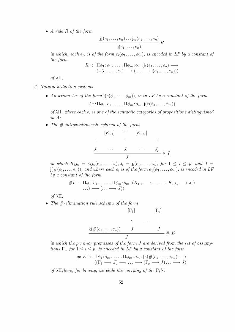
• A rule R of the form

j1(e1, . . . , en) . . . jm(e1, . . . , en)R

j(e1, . . . , en)

in which, each ei, is of the form ei(φ1, . . . , φm), is encoded in LF by a constant ofthe form

R : Πφ1 :o1 . . . . .Πφm :om . j1(e1, . . . , en) −→(j2(e1, . . . , en) −→ (. . . −→ j(e1, . . . , en)))

of λΠ;

2. Natural deduction systems:

• An axiom Ax of the form j(e(φ1, . . . , φm)), is in LF by a constant of the form

Ax :Πφ1 :o1 . . . . .Πφm :om . j(e(φ1, . . . , φm))

of λΠ, where each oi is one of the syntactic categories of propositions distinguishedin A;

• The #-introduction rule schema of the form

...

J1

[Ki,1]

· · ·

· · ·...

Ji

[Ki,hi]

· · ·

...

Jp# I

J

in which Ki,hi= ki,hi

(e1, . . . , en), Ji = ji(e1, . . . , en), for 1 ≤ i ≤ p, and J =j(#(e1, . . . , en)), and where each ei is of the form e1(φ1, . . . , φm), is encoded in LFby a constant of the form

#I : Πφ1 :o1, . . . . .Πφm :om . (K1,1 −→ . . . −→ K1,h1 −→ J1). . .) −→ (. . . −→ J))

of λΠ;

• The #-elimination rule schema of the form

k(#(e1, . . . , en))

[Γ1]

...

J

· · ·

[Γp]

...

J# E

J

in which the p minor premisses of the form J are derived from the set of assump-tions Γi, for 1 ≤ i ≤ p, is encoded in LF by a constant of the form

# E : Πφ1 :om . . . . .Πφm :om . (k(#(e1, . . . , em)) −→((Γ1 −→ J) −→ . . . −→ (Γp −→ J) . . . −→ J)

of λΠ(here, for brevity, we elide the currying of the Γi’s).

52

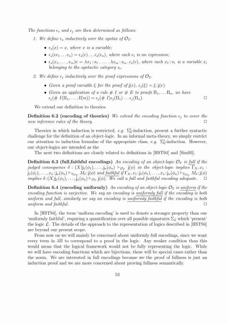
The functions εs and εj are then determined as follows:

1. We define εs inductively over the syntax of OT .

• εs(x) = x, where x is a variable;

• εs(ee1 . . . en) = εs(e) . . . εs(en), where each ei is an expression;

• εs(x1, . . . , xm)e = λx1 : s1 . . . . . λxm : sm . εs(e), where each x1 : s1 is a variable xi

belonging to the syntactic category si.

2. We define εj inductively over the proof expressions of OT .

• Given a proof variable ξ for the proof of j(e), εj(ξ) = ξ : j(e)

• Given an application of a rule # I or # E to proofs Π1, . . .Πn, we haveεj(# I(Π1, . . . ,Π)n)) = εj(# I)εj(Π1) . . . εj(Πn). 2

We extend our definition to theories.

Definition 6.2 (encoding of theories) We extend the encoding function εj to cover thenew inference rules of the theory. 2

Theories in which induction is restricted, e.g. Σ10-induction, present a further syntactic

challenge for the definition of an object-logic. In an informal meta-theory, we simply restrictour attention to induction formulae of the appropriate class, e.g. Σ1

0-induction. However,our object-logics are intended as the

The next two definitions are closely related to definitions in [HST94] and [Sim93].

Definition 6.3 (full,faithful encodings) An encoding of an object-logic OT is full if thejudged consequence δ : (X)j1(φ1), . . . , jn(φn) `OT

j(φ) in the object-logic implies ΓX , x1 :j1(φ1), . . . , xn : jn(φn) `ΣOT

Mδ : j(φ) and faithful if ΓX , x1 : j1(φ1), . . . , xn : jn(φn) `ΣOTMδ : j(φ)

implies δ : (X)j1(φ1), . . . , jn(φn) `OTj(φ). We call a full and faithful encoding adequate. 2

Definition 6.4 (encoding uniformly) An encoding of an object-logic OT is uniform if theencoding function is surjective. We say an encoding is uniformly full if the encoding is bothuniform and full, similarly we say an encoding is uniformly faithful if the encoding is bothuniform and faithful. 2

In [HST94], the term ‘uniform encoding’ is used to denote a stronger property than our‘uniformly faithful’, requiring a quantification over all possible signatures ΣL which ‘present’the logic L. The details of the approach to the representation of logics described in [HST94]are beyond our present scope.

From now on we will mainly be concerned about uniformly full encodings, since we wantevery term in λΠ to correspond to a proof in the logic. Any weaker condition than thiswould mean that the logical framework would not be fully representing the logic. Whilewe will have encoding functions which are bijections, these will be special cases rather thanthe norm. We are interested in full encodings because we the proof of fullness is just aninduction proof and we are more concerned about proving fullness semantically.

53

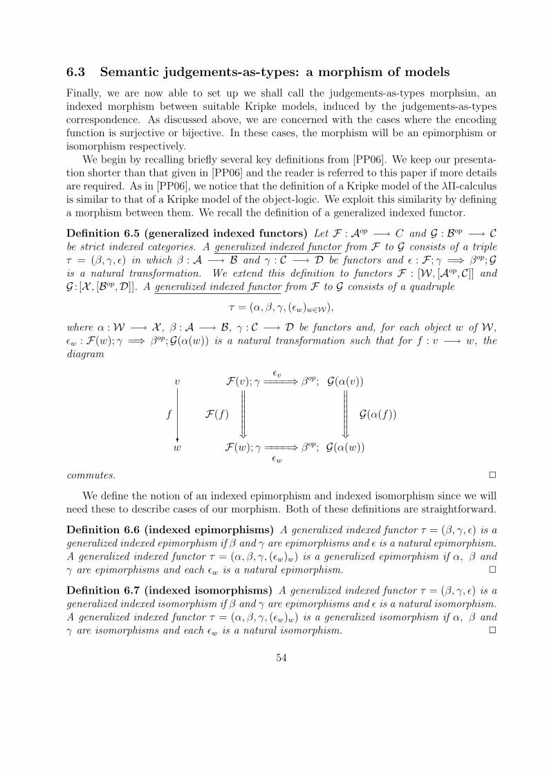
6.3 Semantic judgements-as-types: a morphism of models

Finally, we are now able to set up we shall call the judgements-as-types morphsim, anindexed morphism between suitable Kripke models, induced by the judgements-as-typescorrespondence. As discussed above, we are concerned with the cases where the encodingfunction is surjective or bijective. In these cases, the morphism will be an epimorphism orisomorphism respectively.

We begin by recalling briefly several key definitions from [PP06]. We keep our presenta-tion shorter than that given in [PP06] and the reader is referred to this paper if more detailsare required. As in [PP06], we notice that the definition of a Kripke model of the λΠ-calculusis similar to that of a Kripke model of the object-logic. We exploit this similarity by defininga morphism between them. We recall the definition of a generalized indexed functor.

Definition 6.5 (generalized indexed functors) Let F : Aop −→ C and G : Bop −→ Cbe strict indexed categories. A generalized indexed functor from F to G consists of a tripleτ = (β, γ, ε) in which β : A −→ B and γ : C −→ D be functors and ε : F ; γ =⇒ βop;Gis a natural transformation. We extend this definition to functors F : [W , [Aop, C]] andG : [X , [Bop,D]]. A generalized indexed functor from F to G consists of a quadruple

τ = (α, β, γ, (εw)w∈W),

where α :W −→ X , β : A −→ B, γ : C −→ D be functors and, for each object w of W,εw : F(w); γ =⇒ βop;G(α(w)) is a natural transformation such that for f : v −→ w, thediagram

v F(v); γ ====εv ⇒ βop; G(α(v))

w

f

?F(w); γ

F(f) �wwwwwwww

====εw⇒ βop; G(α(w))

G(α(f))�wwwwwwww

commutes. 2

We define the notion of an indexed epimorphism and indexed isomorphism since we willneed these to describe cases of our morphism. Both of these definitions are straightforward.

Definition 6.6 (indexed epimorphisms) A generalized indexed functor τ = (β, γ, ε) is ageneralized indexed epimorphism if β and γ are epimorphisms and ε is a natural epimorphism.A generalized indexed functor τ = (α, β, γ, (εw)w) is a generalized epimorphism if α, β andγ are epimorphisms and each εw is a natural epimorphism. 2

Definition 6.7 (indexed isomorphisms) A generalized indexed functor τ = (β, γ, ε) is ageneralized indexed isomorphism if β and γ are epimorphisms and ε is a natural isomorphism.A generalized indexed functor τ = (α, β, γ, (εw)w) is a generalized isomorphism if α, β andγ are isomorphisms and each εw is a natural isomorphism. 2

54

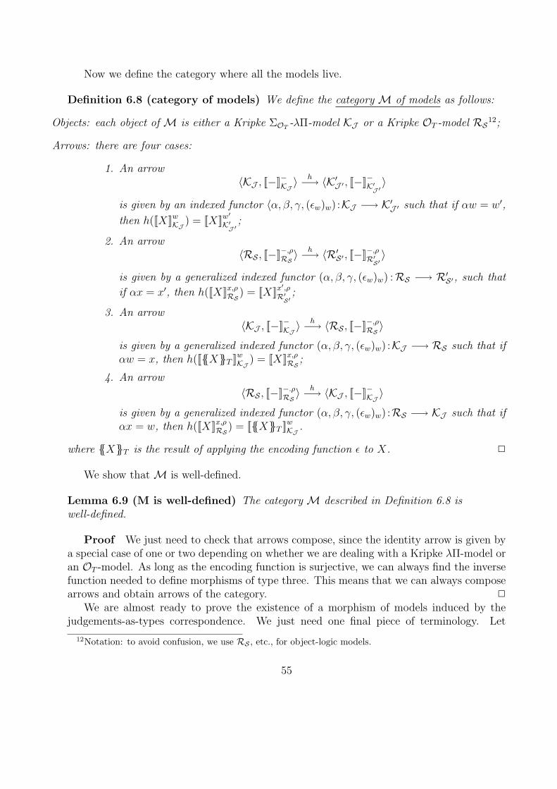
Now we define the category where all the models live.

Definition 6.8 (category of models) We define the category M of models as follows:

Objects: each object of M is either a Kripke ΣOT-λΠ-model KJ or a Kripke OT -model RS12;

Arrows: there are four cases:

1. An arrow〈KJ , [[−]]−KJ 〉

h−→ 〈K′J ′ , [[−]]−K′J ′〉

is given by an indexed functor 〈α, β, γ, (εw)w) :KJ −→ K′J ′ such that if αw = w′,

then h([[X]]wKJ ) = [[X]]w′

K′J ′;

2. An arrow〈RS , [[−]]−,ρ

RS 〉h−→ 〈R′S′ , [[−]]−,ρ

R′S′〉

is given by a generalized indexed functor (α, β, γ, (εw)w) :RS −→ R′S′, such that

if αx = x′, then h([[X]]x,ρRS ) = [[X]]x

′,ρR′S′

;

3. An arrow〈KJ , [[−]]−KJ 〉

h−→ 〈RS , [[−]]−,ρRS 〉

is given by a generalized indexed functor (α, β, γ, (εw)w) :KJ −→ RS such that ifαw = x, then h([[{{X}}T ]]wKJ ) = [[X]]x,ρ

RS ;

4. An arrow

〈RS , [[−]]−.ρRS 〉

h−→ 〈KJ , [[−]]−KJ 〉

is given by a generalized indexed functor (α, β, γ, (εw)w) :RS −→ KJ such that ifαx = w, then h([[X]]x,ρ

RS ) = [[{{X}}T ]]wKJ .

where {{X}}T is the result of applying the encoding function ε to X. 2

We show thatM is well-defined.

Lemma 6.9 (M is well-defined) The category M described in Definition 6.8 iswell-defined.

Proof We just need to check that arrows compose, since the identity arrow is given bya special case of one or two depending on whether we are dealing with a Kripke λΠ-model oran OT -model. As long as the encoding function is surjective, we can always find the inversefunction needed to define morphisms of type three. This means that we can always composearrows and obtain arrows of the category. 2

We are almost ready to prove the existence of a morphism of models induced by thejudgements-as-types correspondence. We just need one final piece of terminology. Let

12Notation: to avoid confusion, we use RS , etc., for object-logic models.

55

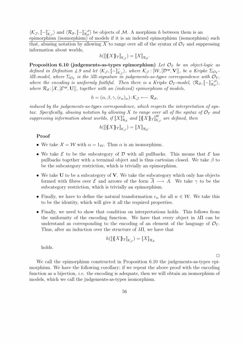
〈KJ , [[−]]−KJ 〉 and 〈RS , [[−]]−,ρRS 〉 be objects ofM. A morphism h between them is an

epimorphism (isomorphism) of models if it is an indexed epimorphism (isomorphism) suchthat, abusing notation by allowing X to range over all of the syntax of OT and suppressinginformation about worlds,

h([[{{X}}T ]]KJ ) = [[X]]RS .

Proposition 6.10 (judgements-as-types epimorphism) Let OT be an object-logic asdefined in Definition 4.9 and let 〈KJ , [[−]]−KJ 〉, where KJ : [W , [Dop,V]], be a Kripke ΣOT

-λΠ-model, where ΣOT

is the λΠ-signature in judgements-as-types correspondence with OT ,where the encoding is uniformly faithful. Then there is a Kripke OT -model, 〈RS , [[−]]−,ρ

RS 〉,where RS : [X , [Eop,U]], together with an (indexed) epimorphism of models,

h = (α, β, γ, (εw)w) :KJ ←− RS ,

induced by the judgements-as-types correspondence, which respects the interpretation of syn-tax. Specifically, abusing notation by allowing X to range over all of the syntax of OT andsuppressing information about worlds, if [[X]]xRS and [[{{X}}T ]]WKJ are defined, then

h([[{{X}}T ]]KJ ) = [[X]]RS .

Proof

• We take X =W with α = 1W . Thus α is an isomorphism.

• We take E to be the subcategory of D with all pullbacks. This means that E haspullbacks together with a terminal object and is thus cartesian closed. We take β tobe the subcategory restriction, which is trivially an epimorphism.

• We take U to be a subcategory of V. We take the subcategory which only has objectsformed with fibres over E and arrows of the form A −→ A. We take γ to be thesubcategory restriction, which is trivially an epimorphism.

• Finally, we have to define the natural transformation εw for all w ∈ W . We take thisto be the identity, which will give it all the required properties.

• Finally, we need to show that condition on interpretations holds. This follows fromthe uniformity of the encoding function. We have that every object in λΠ can beunderstand as corresponding to the encoding of an element of the language of OT .Thus, after an induction over the structure of λΠ, we have that

h([[{{X}}T ]]KJ ) = [[X]]RS

holds.

2

We call the epimorphism constructed in Proposition 6.10 the judgements-as-types epi-morphism. We have the following corollary; if we repeat the above proof with the encodingfunction as a bijection, i.e. the encoding is adequate, then we will obtain an isomorphism ofmodels, which we call the judgements-as-types isomorphism.

56

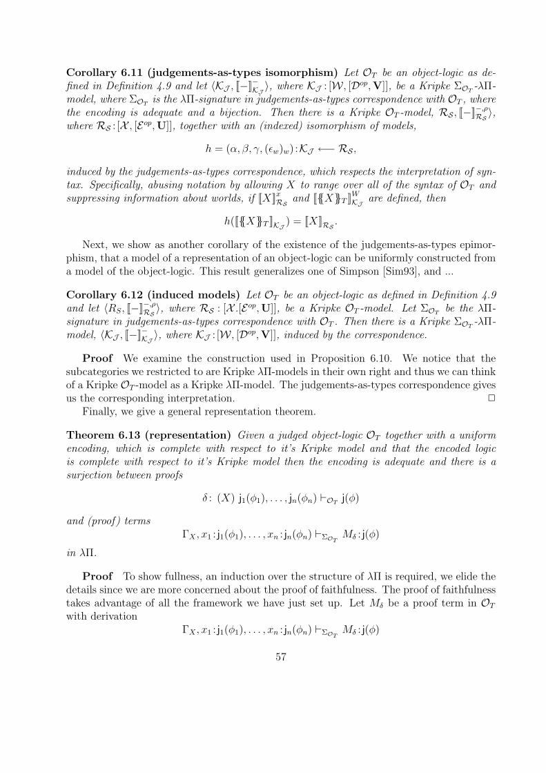
Corollary 6.11 (judgements-as-types isomorphism) Let OT be an object-logic as de-fined in Definition 4.9 and let 〈KJ , [[−]]−KJ 〉, where KJ : [W , [Dop,V]], be a Kripke ΣOT

-λΠ-model, where ΣOT

is the λΠ-signature in judgements-as-types correspondence with OT , wherethe encoding is adequate and a bijection. Then there is a Kripke OT -model, RS , [[−]]−,ρ

RS 〉,where RS : [X , [Eop,U]], together with an (indexed) isomorphism of models,

h = (α, β, γ, (εw)w) :KJ ←− RS ,

induced by the judgements-as-types correspondence, which respects the interpretation of syn-tax. Specifically, abusing notation by allowing X to range over all of the syntax of OT andsuppressing information about worlds, if [[X]]xRS and [[{{X}}T ]]WKJ are defined, then

h([[{{X}}T ]]KJ ) = [[X]]RS .

Next, we show as another corollary of the existence of the judgements-as-types epimor-phism, that a model of a representation of an object-logic can be uniformly constructed froma model of the object-logic. This result generalizes one of Simpson [Sim93], and ...

Corollary 6.12 (induced models) Let OT be an object-logic as defined in Definition 4.9and let 〈RS, [[−]]−,ρ

RS 〉, where RS : [X .[Eop,U]], be a Kripke OT -model. Let ΣOTbe the λΠ-

signature in judgements-as-types correspondence with OT . Then there is a Kripke ΣOT-λΠ-

model, 〈KJ , [[−]]−KJ 〉, where KJ : [W , [Dop,V]], induced by the correspondence.

Proof We examine the construction used in Proposition 6.10. We notice that thesubcategories we restricted to are Kripke λΠ-models in their own right and thus we can thinkof a Kripke OT -model as a Kripke λΠ-model. The judgements-as-types correspondence givesus the corresponding interpretation. 2

Finally, we give a general representation theorem.

Theorem 6.13 (representation) Given a judged object-logic OT together with a uniformencoding, which is complete with respect to it’s Kripke model and that the encoded logicis complete with respect to it’s Kripke model then the encoding is adequate and there is asurjection between proofs

δ : (X) j1(φ1), . . . , jn(φn) `OTj(φ)

and (proof) termsΓX , x1 : j1(φ1), . . . , xn : jn(φn) `ΣOT

Mδ : j(φ)

in λΠ.

Proof To show fullness, an induction over the structure of λΠ is required, we elide thedetails since we are more concerned about the proof of faithfulness. The proof of faithfulnesstakes advantage of all the framework we have just set up. Let Mδ be a proof term in OT

with derivationΓX , x1 : j1(φ1), . . . , xn : jn(φn) `ΣOT

Mδ : j(φ)

57

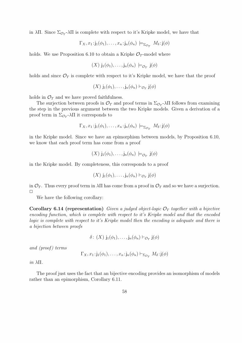
in λΠ. Since ΣOT-λΠ is complete with respect to it’s Kripke model, we have that

ΓX , x1 : j1(φ1), . . . , xn : jn(φn) |=ΣOTMδ : j(φ)

holds. We use Proposition 6.10 to obtain a Kripke OT -model where

(X) j1(φ1), . . . , jn(φn) |=OTj(φ)

holds and since OT is complete with respect to it’s Kripke model, we have that the proof

(X) j1(φ1), . . . , jn(φn) `OTj(φ)

holds in OT and we have proved faithfulness.The surjection between proofs in OT and proof terms in ΣOT

-λΠ follows from examiningthe step in the previous argument between the two Kripke models. Given a derivation of aproof term in ΣOT

-λΠ it corresponds to

ΓX , x1 : j1(φ1), . . . , xn : jn(φn) |=ΣOTMδ : j(φ)

in the Kripke model. Since we have an epimorphism between models, by Proposition 6.10,we know that each proof term has come from a proof

(X) j1(φ1), . . . , jn(φn) |=OTj(φ)

in the Kripke model. By completeness, this corresponds to a proof

(X) j1(φ1), . . . , jn(φn) `OTj(φ)

in OT . Thus every proof term in λΠ has come from a proof in OT and so we have a surjection.2

We have the following corollary:

Corollary 6.14 (representation) Given a judged object-logic OT together with a bijectiveencoding function, which is complete with respect to it’s Kripke model and that the encodedlogic is complete with respect to it’s Kripke model then the encoding is adequate and there isa bijection between proofs

δ : (X) j1(φ1), . . . , jn(φn) `OTj(φ)

and (proof) termsΓX , x1 : j1(φ1), . . . , xn : jn(φn) `ΣOT

Mδ : j(φ)

in λΠ.

The proof just uses the fact that an bijective encoding provides an isomorphism of modelsrather than an epimorphism, Corollary 6.11.

58

7 Representation Theorems

7.1 Introduction

All the previous work has been done to allow us to prove representation theorems. Theseare results which tell us which object-logics can be encoded in LF. Rather than dealing withindividual object-logics as in the literature, [AHMP92, HHP93], we have dealt with generalclasses of object-logics. We have done this to avoid being ad-hoc as well as allowing us todevelop not just representation theorems but a theory of representation. In the later sections,we deal with more specific classes of object-logics obtained through repeating the previouswork with respect to labelled deductive systems.

There are two aspects to a representation theorem, both of which are concerned with therelationship between a proof in the object logic and a derivation of a proof term in λΠ:

1. The first condition is characterized by properties of the encoding. A full encodingmeans that

(X) j1(φ1), . . . , jn(φn) `OTj(φ)

impliesΓX , x1 : j1(φ1), . . . , xn : jn(φn) `ΣOT

Mδ : j(φ)

while a faithful encoding means the opposite implication holds. A full and faithfulencoding is adequate.

2. The second is a more direct relationship between the proof and the proof terms. Weare interested in any properties that a map between them might have, i.e. is it asurjection or bijection.

Proving that an encoding is full is just an induction proof and is relatively straightforward.We are not concerned with proving fullness because we are interested in the semantics ofthe object-logic and λΠ. Analyzing the semantics is done with the aim of providing proofsof faithfulness. The current proofs of faithfulness have been done proof-theoretically. Thiscan be difficult since the proof involves showing that any derivation in λΠis essentiallythe representation of a derivation in the object-logic. Faithfulness should be easy to provesemantically, it should follow from the truth of derivations in λΠ. In fact, the proof ofTheorem 6.13 shows how straightforward it can be although we did a lot of work to getthere.

The relationship between proof terms and proofs is again something which is fairlystraightforward to prove semantically. The morphism induced between the Kripke mod-els, e.g. Theorem 6.10, provides the strength of this map. This is clear with the way theproof was constructed.

In this section, we will study what properties are required to obtain a faithful encodingand examine what effect different properties of the encoding function have on the aboveproperties. The above analysis and the proof of Theorem 6.13 show us that there is arelationship between the two properties.

59

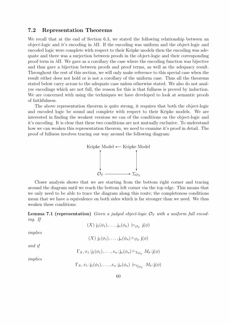
7.2 Representation Theorems

We recall that at the end of Section 6.3, we stated the following relationship between anobject-logic and it’s encoding in λΠ. If the encoding was uniform and the object-logic andencoded logic were complete with respect to their Kripke models then the encoding was ade-quate and there was a surjection between proofs in the object-logic and their correspondingproof term in λΠ. We gave as a corollary the case where the encoding function was bijectiveand thus gave a bijection between proofs and proof terms, as well as the adequacy result.Throughout the rest of this section, we will only make reference to this special case when theresult either does not hold or is not a corollary of the uniform case. Thus all the theoremsstated below carry across to the adequate case unless otherwise stated. We also do not anal-yse encodings which are not full, the reason for this is that fullness is proved by induction.We are concerned with using the techniques we have developed to look at semantic proofsof faithfulness.

The above representation theorem is quite strong, it requires that both the object-logicand encoded logic be sound and complete with respect to their Kripke models. We areinterested in finding the weakest versions we can of the conditions on the object-logic andit’s encoding. It is clear that these two conditions are not mutually exclusive. To understandhow we can weaken this representation theorem, we need to examine it’s proof in detail. Theproof of fullness involves tracing our way around the following diagram:

Kripke Model � Kripke Model

OT

?

6

- ΣOT

?

6

Closer analysis shows that we are starting from the bottom right corner and tracingaround the diagram until we reach the bottom left corner via the top edge. This means thatwe only need to be able to trace the diagram along this route; the completeness conditionsmean that we have a equivalence on both sides which is far stronger than we need. We thusweaken these conditions:

Lemma 7.1 (representation) Given a judged object-logic OT with a uniform full encod-ing. If

(X) j1(φ1), . . . , jn(φn) |=OTj(φ)

implies(X) j1(φ1), . . . , jn(φn) `OT

j(φ)

and ifΓX , x1 : j1(φ1), . . . , xn : jn(φn) `ΣOT

Mδ : j(φ)

impliesΓX , x1 : j1(φ1), . . . , xn : jn(φn) |=ΣOT

Mδ : j(φ)

60

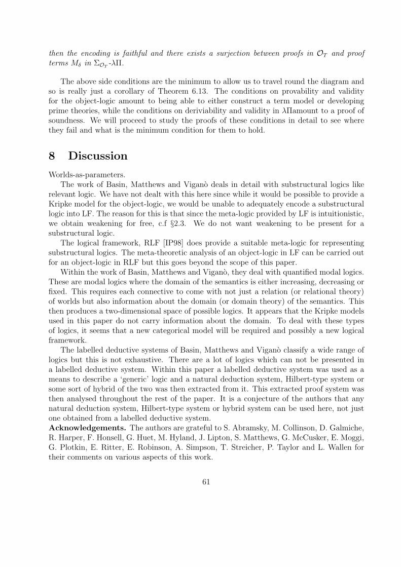
then the encoding is faithful and there exists a surjection between proofs in OT and proofterms Mδ in ΣOT

-λΠ.

The above side conditions are the minimum to allow us to travel round the diagram andso is really just a corollary of Theorem 6.13. The conditions on provability and validityfor the object-logic amount to being able to either construct a term model or developingprime theories, while the conditions on deriviability and validity in λΠamount to a proof ofsoundness. We will proceed to study the proofs of these conditions in detail to see wherethey fail and what is the minimum condition for them to hold.

8 Discussion

Worlds-as-parameters.The work of Basin, Matthews and Vigano deals in detail with substructural logics like

relevant logic. We have not dealt with this here since while it would be possible to provide aKripke model for the object-logic, we would be unable to adequately encode a substructurallogic into LF. The reason for this is that since the meta-logic provided by LF is intuitionistic,we obtain weakening for free, c.f §2.3. We do not want weakening to be present for asubstructural logic.

The logical framework, RLF [IP98] does provide a suitable meta-logic for representingsubstructural logics. The meta-theoretic analysis of an object-logic in LF can be carried outfor an object-logic in RLF but this goes beyond the scope of this paper.

Within the work of Basin, Matthews and Vigano, they deal with quantified modal logics.These are modal logics where the domain of the semantics is either increasing, decreasing orfixed. This requires each connective to come with not just a relation (or relational theory)of worlds but also information about the domain (or domain theory) of the semantics. Thisthen produces a two-dimensional space of possible logics. It appears that the Kripke modelsused in this paper do not carry information about the domain. To deal with these typesof logics, it seems that a new categorical model will be required and possibly a new logicalframework.

The labelled deductive systems of Basin, Matthews and Vigano classify a wide range oflogics but this is not exhaustive. There are a lot of logics which can not be presented ina labelled deductive system. Within this paper a labelled deductive system was used as ameans to describe a ‘generic’ logic and a natural deduction system, Hilbert-type system orsome sort of hybrid of the two was then extracted from it. This extracted proof system wasthen analysed throughout the rest of the paper. It is a conjecture of the authors that anynatural deduction system, Hilbert-type system or hybrid system can be used here, not justone obtained from a labelled deductive system.Acknowledgements. The authors are grateful to S. Abramsky, M. Collinson, D. Galmiche,R. Harper, F. Honsell, G. Huet, M. Hyland, J. Lipton, S. Matthews, G. McCusker, E. Moggi,G. Plotkin, E. Ritter, E. Robinson, A. Simpson, T. Streicher, P. Taylor and L. Wallen fortheir comments on various aspects of this work.

61

References

[Acz78] Peter Aczel. The type theoretic interpretation of constructive set theory. InLogic Colloquium 1977, pages 55–66. North-Holland Publishing Company, 1978.

[Acz80] Peter Aczel. Frege structures and the notions of proposition, truth and set. InJ. Barwise, H.J.Keisler, and K. Kunen, editors, The Kleene Symposium, pages31–59. North-Holland Publishing Company, 1980.

[AHMP92] Arnon Avron, Furio Honsell, Ian Mason, and Randy Pollack. Using typed lambdacalculus to implement formal systems on a machine. Journal of Automated Rea-soning, 9:309–354, 1992.

[AHMP98] Arnon Avron, Furio Honsell, Marion Miculan, and Cristian Paravano. Encodingmodal logics in logical frameworks. Studia Logica, 60:161–208, 1998.

[Avr91] Arnon Avron. Simple consequence relations. Information and Computation,92:105–139, 1991.

[BMV96] David Basin, Sean Matthews, and Luca Vigano. Implementing modal and rele-vance logics in a logical framework. In L.C. Aiello, J. Doyle, and S.C. Shapiro,editors, Principles of Knowledge Representation and Reasoning: Proceedings ofthe Fifth International Conference (KR ’96), pages 386–397. Morgan KaufmannPublishers, San Francisco, CA, 1996.

[BMV97] David Basin, Sean Matthews, and Luca Vigano. Labelled propositional modallogics: theory and practice. Journal of Logic and Computation, 7(1):685–717,1997.

[BMV98] David Basin, Sean Matthews, and Luca Vigano. Natural deduction for non-classical logics. studia logica, 60(1):119–160, 1998.

[Gar92] Philippa Gardner. Representing Logics in Type Theory. PhD thesis, Universityof Edinburgh, 1992.

[Gen34] Gerhard Gentzen. Untersuchungen uber das logische schliessen. MathematischeZeitschrift, 39:176–210,405–431, 1934.

[Gir87] Jean-Yves Girard. Linear logic. Theoretical Computer Science, 50(1):1–102,1987.

[HHP87] Robert Harper, Furio Honsell, and Gordon Plotkin. A framework for defininglogics. In Proceedings 2nd Annual IEEE Symp. on Logic in Computer Science,LICS’87, Ithaca, NY, USA, 22–25 June 1987, pages 194–204. IEEE ComputerSociety Press, New York, 1987.

62

[HHP93] Robert Harper, Furio Honsell, and Gordon Plotkin. A framework for defininglogics. Journal of the Association for Computing Machinery, 40(1):143–184,1993.

[Hod01] Wilfred Hodges. Elementary predicate logic. In Dov Gabbay and Franz Guen-thner, editors, Handbook of Philosophical Logic, volume 1. Kluwer AcademicPublishers, 2001.

[HST94] Robert Harper, Donald Sannella, and Andrzej Tarlecki. Structured theory pre-sentations and logic representations. Annals of Pure and Applied Logic, 67(1-3):113–160, 1994.

[IP98] Samin S. Ishtiaq and David J. Pym. A relevant analysis of natural deduction.Journal of Logic and Computation, 8(6):809–838, 1998.

[IP02] Samin Ishtiaq and David J. Pym. Dependently-typed, bunched λ-calculus. Jour-nal of Logic and Computation, 12(6):1061–1104, 2002.

[Kan00] Immanuel Kant. Immanuel Kants Logik: Ein Hanbuch zu Vorlesungen. GottlobBenjamin Jasche, Konigsberg, 1800.

[Kri63] Saul A. Kripke. Semantical analysis of modal logic I. Zeitschrift fur mathematicheLogik und Grundlagen der Mathematik, 16:83–94, 1963.

[LS86] Joachim Lambek and Phil Scott. Introduction to Higher Order Categorical Logic.Cambridge University Press, 1986.

[ML71] Per Martin-Lof. Hauptsatz for the intuitionistic theory of iterated inductivedefinitions. In J. E. Fenstad, editor, Second Scandinavian Logic Symposium.North-Holland, 1971.

[ML75] Per Martin-Lof. An intutionistic theory of types: Predicative part. In H.E.Rose and J.C. Shepherdson, editors, Logic Colloquim 1973, pages 73–188. North-Holland Publishing Company, 1975.

[ML82] Per Martin-Lof. On the meanings of the logical constants and the justificationsof the logical laws, 1982.

[ML85] Per Martin-Lof. On the meanings of logical constants and the justification of thelogical laws. Technical report, Scuola di Specializzazione in Logica Matematica,Dipartimento di Matematica, Universita di Siena, 1985. Technical Report 2.

[MM91] John C. Mitchell and Eugenio Moggi. Kripke-style models for typed lambdacalculus. Annals of Pure and Applied Logic, 51:99–124, 1991.

[nDCH96] L. Fari nas Del Cerro and A. Herzig. Combining classical and intuitionistic logic.In F. Baader and K.U. Schulz, editors, Frontiers of Combining Systems, pages93–102. Kluwer, 1996.

63

[Pfe95] Frank Pfenning. Structural cut elimination. In D. Kozen, editor, Proceedingsof the Tenth Annual Symposium on Logic in Computer Science, pages 156–166.IEEE Computer Society Press, 1995.

[PP06] David J. Pym and Mark A. Price. Functorial kripke-beth-joyal models of theλΠ-calculus I: type theory and internal logic. www.cs.bath.ac.uk/MPrice/

downloads/Kripke1.ps, 2006.

[Pra65] Dag Prawitz. Natural Deduction: A Proof-Theoretic Study. Almquist and Wik-sell, 1965.

[Pym90] David J. Pym. Proofs, Search and Computation in General Logic. PhD thesis,University of Edinburgh, 1990.

[Pym01] David J. Pym. Functorial kripke-beth-joyal models of the λΠ-calculus III: logicprogramming and its semantics. www.cs.bath.ac.uk/~pym/kripke3.ps, 2001.

[Rea88] Stephen Read. Relevant Logic. Blackwell, 1988.

[SHD93] Peter Schroder-Heister and Kosta Dosen, editors. Substructural Logics. Claren-don Press, 1993.

[Sim93] Alex Simpson. Kripke semantics for a logical framework. homepages.inf.edu.ac.uk/als/Research/kripke.ps.gz, 1993.

[Sun01] Goran Sundholm. Systems of deduction. In Dov Gabbay and Franz Guenthner,editors, Handbook of Philosophical Logic, volume 2. Kluwer Academic Publishers,2001.

[Vig00] Luca Vigano. Labelled Non-Classical Logics. Kluwer Academic Publishers, 2000.

64