LUND UNIVERSITY

DEPT. OF CHEMICAL ENGINEERING

KET050 FEASIBILITY STUDIES ON INDUSTRIAL PLANTS

FINAL REPORT

ON

PURIFICATION OF GREEN METHANOL

FROM PULP PRODUCTION

PRESENTED TO

INVICO METHANOL

PRINCIPAL INVESTIGATORS:

RISHI MIDHA, KALEY OGILVY, TAYLOR SKINGLE, CAROLYN BUCHANAN, GRAHAM MANTAY

TUTOR:

OLA WALLBERG

JUNE/2015

i

Abstract

Invico Methanol, an engineering company, works to provide different methods of creating

“green” energy. Invico has recently created a process that utilizes liquid-liquid extraction of raw

methanol in order to remove compounds containing sulfur as well as recover the solvent and

methanol from the extraction. Invico has successfully verified parts of this process in pilot scale.

However, the aim is to design full-scale equipment.

The purpose of this project was to complete an in-depth analysis and perform a technical-

economical comparison of the extraction and purification of methanol from a pulp mill.

Methanol that can be exported from a kraft pulp mill can be used for bio-diesel production, thus

lowering the environmental impact of the plant through creating a biofuel. This report covers

various issues including process designs of our suggested process and other competing

processes. Our recommended design consists of a methanol cleaning system with two

distillation columns, a liquid-liquid extraction column, and an oil cleaning system for cost

reduction, which is achieved using a stream stripper. Each of these designs were simulated and

evaluated with Aspen Plus V8.2 software, which solved the material and energy balances

involved in the process. An investment and operating cost evaluation was also completed, and

the total determined fixed plant cost is 61.3 million SEK and the total operating annual cost is

43.0 million SEK. Lastly, a sensitivity analysis was completed to understand how the selling price

of the reduced methanol, the cost of extraction oil, the interest rate, and maintenance costs

impacted the plant value. The sensitivity analysis showed that at the expected interest rate and

maintenance costs of 11% and 6% (of total plant cost) respectively, the value of the plant would

not be damaged too greatly. More importantly, it was determined that both the selling price of

methanol and the cost of the extraction oil have the power to make this project completely

viable or quite unviable. It is expected that since biofuels are not yet in very high demand, and

the quality of the produced biofuel is not likely to meet the standards of regular methanol, the

selling price of the methanol is likely to be below average and have a significant negative impact

on profits. However, due to the oil cleaning system, if a low-cost extraction oil is found and used

for this process, it has the capability to offset the expected losses from the low selling-point of

the methanol, especially for the first few ‘testing’ years of the project.

Final recommendations would include much more detailed research with regards to variable

costs and selling prices, and the investigation of a water cleaning system for the steam and water

waste streams, as if they are reused, variable costs could be reduced significantly.

ii

Table of Contents

ABSTRACT ........................................................................................................................................ I

TABLE OF CONTENTS ....................................................................................................................... II

LIST OF TABLES .............................................................................................................................. III

INTRODUCTION .............................................................................................................................. 1

The Pulping Process.................................................................................................................................................................. 1

The Kraft Process ....................................................................................................................................................................... 2

PROCESS OVERVIEW ....................................................................................................................... 3

Boiler .............................................................................................................................................................................................. 4

Distillation Column 1 ................................................................................................................................................................ 4

Inline Mixer 1 .............................................................................................................................................................................. 5

Extraction Column ..................................................................................................................................................................... 5

Distillation Column 2 ................................................................................................................................................................ 7

Oil Cleaning System ................................................................................................................................................................... 9

Decanter Modelling ................................................................................................................................................................ 10

PROCESS ALTERNATIVES ............................................................................................................... 12

MATERIALS AND EQUIPMENT SIZING ............................................................................................ 13

Distillation Column Sizing ................................................................................................................................................... 13

Extraction Column Sizing ..................................................................................................................................................... 15

Steam Stripper ......................................................................................................................................................................... 16

Mixer and Pump ...................................................................................................................................................................... 17

Heat Exchangers ...................................................................................................................................................................... 17

INVESTMENT COST ANALYSIS ........................................................................................................ 18

Plant Cost ................................................................................................................................................................................... 18

Operating Cost.......................................................................................................................................................................... 19

iii

SENSITIVITY ANALYSIS AND FEASIBILITY STUDY ............................................................................. 24

Methanol Sale Price ................................................................................................................................................................ 26

Extraction Oil Price ................................................................................................................................................................ 28

Interest Rate ............................................................................................................................................................................. 30

Maintenance Costs .................................................................................................................................................................. 31

CONCLUSIONS AND RECOMMENDATIONS .................................................................................... 33

BIBLIOGRAPHY.............................................................................................................................. 36

APPENDIX ..................................................................................................................................... 38

Sample Calculations ............................................................................................................................................................... 38 Distillation Column Design Procedure ............................................................................................................................................ 38 Distillation Column/Steam Stripper Dimensions ...................................................................................................................... 38 Extraction Column Diameter ............................................................................................................................................................... 40 Surface Area for Heat Exchange ......................................................................................................................................................... 40 NPV Calculation ......................................................................................................................................................................................... 41

Data Tables ................................................................................................................................................................................ 41 Plant Costs (Ulrich Estimations) ........................................................................................................................................................ 41 Stream Conditions .................................................................................................................................................................................... 44 Unit Operating Conditions .................................................................................................................................................................... 49 Economic Tables and Investment Calculations........................................................................................................................... 51

List of Tables

Table 1: Feed conditions of the raw material to purified, and the physical properties of each component _________ 1 Table 2: Stream conditions before and after the first distillation column, with stream S1 representing the incoming vapour stream, S2 representing the liquid top stream, and S3 representing the liquid bottoms stream ____________________________________________________________________________________________________________________ 5 Table 3: Stream conditions before and after the extraction column, with stream S5 representing the incoming diluted liquid stream, S8 representing the incoming oil (n-hexadecane) stream, S9 representing the oil-heavy top stream, and S10 representing the refined bottoms stream. _______________________________________________________ 6 Table 4: Stream conditions before and after the second distillation column, with stream S10 representing the incoming purified liquid stream S11 representing the final product stream to be shipped to storage, and S12 representing the a waste stream of primarily water. __________________________________________________________________ 7 Table 5: Detailed Aspen results of the final product stream ___________________________________________________________ 8 Table 6: Stream conditions before and after the steam striper, with stream S20 representing the incoming contaminated oil-heavy liquid, STEAMSTR representing the pure steam stream used for stripping, STRIPTOP representing the waste vapour stream, and STRIPBOT representing the cleaned oil, to be recycled back to the extraction column ______________________________________________________________________________________________________ 10 Table 7: NRTL model binary parameters for α-pinene (1) and water (2). The first set of data is extracted from a paper on liquid-liquid equilibrium for binary mixtures (Utami, Sutijan, Roto, & Sediawan, Liquid-Liquid Equilibrium for the Binary Mixtures of Alpha-Pinene+Water+Alpha-Terpineol+Water, 2013). The second set of data is extracted from a paper on liquid-liquid equilibrium for three component systems (Utami, Sutijan,

iv

Roto, & Sediawan, Liquid-Liquid Equilibrium for System Composed of Alpha-Pinene, Alpha-Terpineol and Water, 2013). ___________________________________________________________________________________________________________ 11 Table 8: Summary of Distillation Column Design Parameters _______________________________________________________ 14 Table 9: List of variables used in Equation 4, their meaning, and units _____________________________________________ 15 Table 10: Summary of Steam Stripper Design Parameters ___________________________________________________________ 16 Table 11: Determined power requirements for the two inline mixer and the centrifugal pump, based off of Aspen results and the flow being handled (Silverson, 2015) _________________________________________________________ 17 Table 12: Summary of Heat Exchanger Design Parameters (Teralba, 2015) _______________________________________ 18 Table 13: Ulrich Cost Estimation for Distillation Column 1 (EconExpert, 2000) ____________________________________ 19 Table 14: Summary of fixed plant installation and equipment cots, and a final plant cost _________________________ 19 Table 15: Average Heating Oil Costs ___________________________________________________________________________________ 20 Table 16: Summary of operating costs of plant employees ___________________________________________________________ 21 Table 17: Estimation of income from methanol production __________________________________________________________ 21 Table 18: Summary of storage costs for products and feed __________________________________________________________ 23 Table 19: Total annual operating costs for the plant _________________________________________________________________ 24 Table 20: Factors Affecting Net Present Value ________________________________________________________________________ 25 Table 21: Summary of Reference NPV Conditions ____________________________________________________________________ 26 Table 22: Summary of Costs____________________________________________________________________________________________ 34 Table 23: Physical parameters of the two phases in the extraction column (Sigma Aldrich, 2014) ________________ 40 Table 24: Ulrich cost estimation for Distillation Column 2 (EconExpert, 2000) _____________________________________ 41 Table 25: Ulrich cost estimation for Inline Mixer 1 and 2 (EconExpert, 2000) ______________________________________ 42 Table 26: Ulrich cost estimation for the centrifugal pump (EconExpert, 2000) _____________________________________ 42 Table 27: Ulrich cost estimation for Heat Exchanger B13 (EconExpert, 2000) _____________________________________ 43 Table 28: Ulrich cost estimation for Heat Exchanger B6 (EconExpert, 2000) _______________________________________ 43 Table 29: Ulrich cost estimation for the Steam Stripper (EconExpert, 2000) _______________________________________ 44 Table 30: Ulrich cost estimation for the Extraction Column (EconExpert, 2000) ___________________________________ 44 Table 31: Detailed stream conditions for S1-S12 _____________________________________________________________________ 45 Table 32: Detailed stream conditions for S14-WATER2 ______________________________________________________________ 47 Table 33: Summary of Factors affecting NPV _________________________________________________________________________ 51 Table 34: NPV and Pay off time calculation summary ________________________________________________________________ 52

1

Introduction The purpose of this project is to explore the possibility of cleaning the effluent from the Kraft

pulping process, by isolating methanol and ethanol from water, α-pinene, acetone and various

sulfur-containing compounds. The recovered methanol and ethanol can be used to produce bio-

diesel, an alternative fuel source, potentially used for transportation or as fuel for the kraft

pulping process. This area of study is valuable as the demand for eco-friendly alternatives to

fossil fuel is growing rapidly. For this project to be successful the resulting methanol must meet

industrial standards with regards to sulphur content, and the operating/investment costs of the

process must be justifiable. The pulp mill effluent content has been pre-determined, and is given

by Table 1, which also includes physical properties of the effluent components.

Table 1: Feed conditions of the raw material to purified, and the physical properties of each component

Chemical Methanol Ethanol Turpentine Acetone DMS DMDS Ammonia Water

Percent of Feed, by Weight

(%)

78.8 3.1 12.1 0.8 0.4 0.3 0 4.6

Boiling Point (°C)

64.7 78.37 90-115 56 37 110 -33.34 100

Molecular Weight (g/mol)

32.04 46.07 136 58.08 62.1 94.20 17.03 18.02

Density (kg/m3)

791.80 789.00 854-868 791.00 846 1060 0.73 999.97

The industrial standard, generally speaking, requires the water content of the methanol product

to be 0.1%, by mass, or less, and the sulfur content to be reduced to 10 ppm or less. The

turpentine must be completely removed.

In this report, existing methanol cleaning techniques will be evaluated, compared, and utilized to

formulate a potentially unique process for methanol purification. To analyze the viability of the

formulated design, an Aspen model will be created, and dimensioning, cost analysis, and

feasibility studies will be conducted.

The Pulping Process

The pulping process is a method of turning materials from wood products (sawmill residue, logs

and chips, recycled paper) into pulp, which can be delivered to a paper mill for further

processing. Wood-based materials entering a pulp mill consist of cellulose fibers, lignin, and

hemicelluloses. The pulp product primarily consists of cellulose fibers, which are the desirable

2

component for paper production. Lignin serves the purpose of binding the cellulose fibers

together. In its simplest form, the pulping process is the act of degrading the lignin and the bulk

structure of the incoming wood material, leaving behind pure cellulose fiber material. This can

be achieved by mechanical or chemical means. The mechanical method involves physically

ripping wood fibers apart. The general chemical method involves chemically breaking down the

structure of the lignin and hemicellulose into a water-soluble compound, which can then be

washed away from the cellulose fibers. Over 80% of global pulp production is achieved using the

kraft method, which is a chemical process (European Paper & Packaging Industries, 2015).

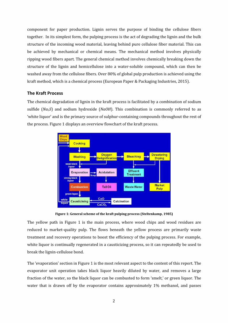
The Kraft Process

The chemical degradation of lignin in the kraft process is facilitated by a combination of sodium

sulfide (Na2S) and sodium hydroxide (NaOH). This combination is commonly referred to as

‘white liquor’ and is the primary source of sulphur-containing compounds throughout the rest of

the process. Figure 1 displays an overview flowchart of the kraft process.

Figure 1: General scheme of the kraft pulping process (Steltenkamp, 1985)

The yellow path in Figure 1 is the main process, where wood chips and wood residues are

reduced to market-quality pulp. The flows beneath the yellow process are primarily waste

treatment and recovery operations to boost the efficiency of the pulping process. For example,

white liquor is continually regenerated in a causticizing process, so it can repeatedly be used to

break the lignin-cellulose bond.

The ‘evaporation’ section in Figure 1 is the most relevant aspect to the content of this report. The

evaporator unit operation takes black liquor heavily diluted by water, and removes a large

fraction of the water, so the black liquor can be combusted to form ‘smelt,’ or green liquor. The

water that is drawn off by the evaporator contains approximately 1% methanol, and passes

3

through a sequence of distillation columns and filters to bring it to the composition given by

Table 1. A box diagram outlining the distillation process is shown by Figure 2.

Figure 2: Post-evaporation recovery of methanol in the kraft process. Addition of H2SO4 during pre-treatment lowers the pH of the stream, removing H2S and CH4S as gasses, and forming an (NH4)2SO4 precipitate. The

stripper column usually contains 20 trays, and the methanol distillation column contains 15 trays.

It can be seen that following the process given by Figure 2, the outlet conditions are the same as

those shown in Table 1. From this point, the stream enters the section of the process that is

designed and evaluated in this report.

Process Overview The proposed process consists of six unit operations, each which plays a role in producing a

purified methanol stream by removing any undesirable components. The initial stream, as

determined previously, contains methanol, ethanol, DMS, DMDS, Acetone, Turpentine (α-

pinene), ammonia, and water. Roughly 0.25 kilograms per minute of effluent are fed into the

system, which translates to around 19 liters per minute. The finalized recommended process to

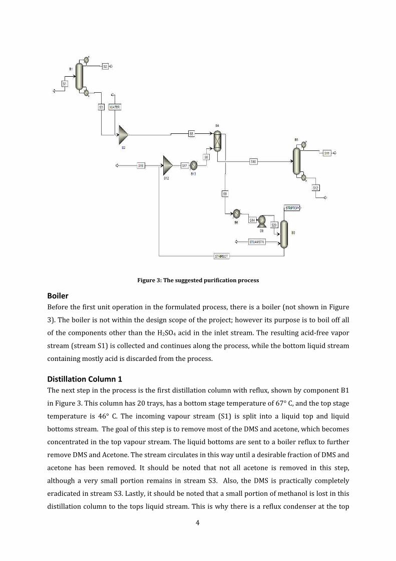
achieve the goals as outlined in the Introduction section is shown by Figure 3. Throughout this

section, numerous tables are used to display the stream and operating conditions data for the

specified process. All of the detailed raw data tables are shown in the Unit Operations Section

and Stream Conditions Section in the Appendix.

4

Figure 3: The suggested purification process

Boiler Before the first unit operation in the formulated process, there is a boiler (not shown in Figure

3). The boiler is not within the design scope of the project; however its purpose is to boil off all

of the components other than the H2SO4 acid in the inlet stream. The resulting acid-free vapor

stream (stream S1) is collected and continues along the process, while the bottom liquid stream

containing mostly acid is discarded from the process.

Distillation Column 1 The next step in the process is the first distillation column with reflux, shown by component B1

in Figure 3. This column has 20 trays, has a bottom stage temperature of 67° C, and the top stage

temperature is 46° C. The incoming vapour stream (S1) is split into a liquid top and liquid

bottoms stream. The goal of this step is to remove most of the DMS and acetone, which becomes

concentrated in the top vapour stream. The liquid bottoms are sent to a boiler reflux to further

remove DMS and Acetone. The stream circulates in this way until a desirable fraction of DMS and

acetone has been removed. It should be noted that not all acetone is removed in this step,

although a very small portion remains in stream S3. Also, the DMS is practically completely

eradicated in stream S3. Lastly, it should be noted that a small portion of methanol is lost in this

distillation column to the tops liquid stream. This is why there is a reflux condenser at the top

5

stream, to minimize the loss of desirable compounds. The boilup ratio and condenser reflux ratio

have been optimized to minimize methanol losses, and to maximize the removal of acetone and

DMS. The technical specifications of Distillation Column 1 are shown in the Unit Operating

Conditions heading in the Appendix section. Table 2 outlines the relevant stream conditions

with respect to Distillation Column 1. The bottoms stream is then passed onto the next step of

the process.

Table 2: Stream conditions before and after the first distillation column, with stream S1 representing the incoming vapour stream, S2 representing the liquid top stream, and S3 representing the liquid bottoms

stream

Stream S1 S2 S3 Phase: Vapour Liquid Liquid

Component Mole Flow Units methanol KMOL/HR 24.56 0.2456 24.32 ethanol KMOL/HR 0.6729 trace 0.6729 acetone KMOL/HR 0.1377 0.1347 0.003065

DMS KMOL/HR 0.06438 0.06437 trace DMDS KMOL/HR 0.03185 trace 0.03185

α-pinene KMOL/HR 0.8882 trace 0.8878 water KMOL/HR 2.553 trace 2.553

Inline Mixer 1 The bottoms liquid stream from Distillation Column 1 (Stream S3 in Figure 3) is passed to an

inline mixer (component B2 in Figure 3) where it is diluted with water, reducing the stream

from approximately 85% methanol content to 71% methanol content. An inline mixer was

selected to provide sufficient mixing of the two liquid streams, thus forming stream S5, prior to

them entering the extraction column. The addition of water in this step is important as it creates

a significant solubility difference in the stream for the following step, which involves a liquid-

liquid extraction to reduce the concentrations of acetone, DMS, DMDS, and turpentine in the

stream. The technical specifications of Inline Mixer 1 are shown by the Unit Operating

Conditions heading in the Appendix section.

Extraction Column Following the Inline Mixer, Stream S5 is passed into an extraction column, which is also fed with

a stream of lightly diluted n-hexadecane (Stream S8). Stream S8 is the resulting stream from the

oil recycle loop, which will be discussed later in the report. This extraction column has a top

stage temperature of 23.7° C and a bottom stage temperature of 19.6° C. The goal of this liquid-

liquid extraction is primarily to reduce the concentrations of α-pinene and DMDS, although it

also further reduces the concentration of acetone and DMS. Table 3 outlines the relevant stream

6

conditions with respect to the extraction column. Detailed technical specifications for the

extraction column are shown in the Unit Operations Heading in the Appendix section.

Table 3: Stream conditions before and after the extraction column, with stream S5 representing the incoming diluted liquid stream, S8 representing the incoming oil (n-hexadecane) stream, S9 representing the oil-heavy

top stream, and S10 representing the refined bottoms stream.

S5 S8 S9 S10 From B2 B13 B4 B4

To B4 B4 B6 B5 Phase: Liquid Liquid Liquid Liquid

Component Mole Flow Units methanol KMOL/HR 24.32 0 2.714 21.60 ethanol KMOL/HR 0.6729 0 0.08714 0.5857 acetone KMOL/HR 0.003065 0 0.002454 trace

DMS KMOL/HR trace 0 trace trace DMDS KMOL/HR 0.03185 0 0.02794 0.003904

α-pinene KMOL/HR 0.8878 0 0.8875 trace water KMOL/HR 8.104231 0.5582 0.05116 8.611

n-hexadecane KMOL/HR 0 66.24 66.19 0.04741

It can be seen in Table 3 that a significant reduction of α-pinene is achieved with the extraction

column. A fairly significant amount of DMDS and acetone are also removed. Trace amounts of

DMS are removed, although the DMS is already very low in concentration. From the resulting

‘cleaned’ stream (S10) it can be seen that the stream is close to approaching the desired

purification of methanol and ethanol, however there is still a concentration of DMDS that is

above 10 ppm and the water content is above 0.1%. It is therefore still not adequate. The top

stream from the extraction column (S9) primarily consists of n-hexadecanes, and is sent to an

oil-cleaning system so the oil can be reused within the extraction column. This system is

described in future sections.

The importance of the addition of water before the extraction column can be seen from Table 3,

where the α-pinene is almost completely eradicated from the stream. The highly polar nature of

water, paired with the highly non-polar nature of n-hexadecane causes the α-pinene (a non-

polar solvent) to be drawn out of the stream with the exiting liquid stream (S9). In the oil-

cleaning system, Stream S9 will primarily need to be stripped of α-pinene and DMDS. Another

observation from Table 3 is that trace amounts of ethanol and methanol are lost to stream S9 in

the extraction process. It is important to note, though, that following the oil cleaning, this stream

is returned to the extraction process, therefore some of this ethanol and methanol could be

returned to the product stream. The remaining methanol and ethanol removed from the oil

could be recovered using further processing steps; however this is out of the scope of the work

for this report.

7

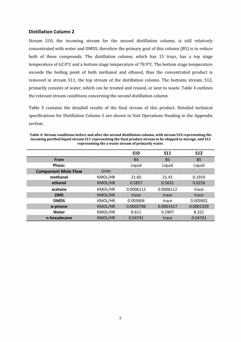
Distillation Column 2

Stream S10, the incoming stream for the second distillation column, is still relatively

concentrated with water and DMDS, therefore the primary goal of this column (B5) is to reduce

both of these compounds. The distillation column, which has 15 trays, has a top stage

temperature of 62.0°C and a bottom stage temperature of 78.9°C. The bottom stage temperature

exceeds the boiling point of both methanol and ethanol, thus the concentrated product is

removed in stream S11, the top stream of the distillation column. The bottoms stream, S12,

primarily consists of water, which can be treated and reused, or sent to waste. Table 4 outlines

the relevant stream conditions concerning the second distillation column.

Table 5 contains the detailed results of the final stream of this product. Detailed technical

specifications for Distillation Column 2 are shown in Unit Operations Heading in the Appendix

section.

Table 4: Stream conditions before and after the second distillation column, with stream S10 representing the incoming purified liquid stream S11 representing the final product stream to be shipped to storage, and S12

representing the a waste stream of primarily water.

S10 S11 S12 From B4 B5 B5

Phase: Liquid Liquid Liquid Component Mole Flow Units

methanol KMOL/HR 21.60 21.41 0.1919 ethanol KMOL/HR 0.5857 0.5631 0.0226 acetone KMOL/HR 0.0006112 0.0006112 trace

DMS KMOL/HR trace trace trace DMDS KMOL/HR 0.003904 trace 0.003902

α-pinene KMOL/HR 0.0002746 0.0001417 0.0001329 Water KMOL/HR 8.611 0.2907 8.321

n-hexadecane KMOL/HR 0.04741 trace 0.04741

8

Table 5: Detailed Aspen results of the final product stream

S11 From B5

To Substream: MIXED

Phase: Liquid Component Mass Fraction Units

methanol 0.9565 ethanol 0.03617 acetone trace

DMS trace DMDS trace

α-pinene trace water 0.007302

n-hexadecane trace Mole Flow KMOL/HR 22.26 Mass Flow KG/HR 717.3

Volume Flow L/MIN 15.96 Temperature C 61.99

Pressure BAR 0.9 Vapor Fraction 0 Liquid Fraction 1 Solid Fraction 0

Molar Enthalpy CAL/MOL -56460 Mass Enthalpy CAL/GM -1753 Enthalpy Flow CAL/SEC -349200 Molar Entropy CAL/MOL-K -54.83 Mass Entropy CAL/GM-K -1.702 Molar Density MOL/CC 0.02325 Mass Density GM/CC 0.7489

Average Molecular Weight 32.22

The purified product stream, shown by Table 5, has a very concentrated combined methanol and

ethanol mass fraction of 99.2%. According to the standards introduced in the previous section,

the product stream was required to include less than 0.1% water by mass and less than 10 parts

per million (ppm) of sulfur.

Table 5 confirms that the final mass fraction of sulfur-containing compounds is 3.32x10-7, which

is significantly less than 10 parts per million. The sulfur removal requirement is therefore

achieved. The final water concentration is observed to be 0.7%, by mass, slightly higher than the

desired concentration of 0.1%. After various optimization methods with the boilup and reflux

ratios, the team was unsuccessful in achieving the desired water concentration. A decision had

to be made between adding another distillation column and looking for further improvements to

9

the existing column to achieve the desired concentration. Due to the astronomical cost of adding

another distillation column to achieve such a small purification of the final stream, the team

decided that another column would not be added. Instead, it is recommended that further

research and modelling of this column are completed. It is suspected that finely tuning the

column by changing the type of trays, the number of trays and other variables could achieve the

desired separation. This option seems much more cost effective and reasonable compared to

adding in a second column. Unfortunately, the team did not have the expertise or resources

(time and knowledge) to complete this tuning of the column.

Oil Cleaning System

Stream S9, which exits the extraction column (B4), is highly concentrated in n-hexadecane, thus

providing the opportunity for reuse in the extraction column if it is adequately cleaned. The

removal of undesirable compounds (methanol, ethanol, acetone, DMS, DMDS, α-pinene, water) is

achieved using a steam stripper (B3), which uses steam to remove all of the volatile organic

compounds in the stream and release them as a vapour (Stream STRIPTOP). The resulting

bottoms liquid stream STRIPBOT is almost entirely consisted of n-hexadecane and a small

amount of water. Prior to entering the steam stripper and mixing with high-pressure steam, the

stream passes through a heat exchanger (B6) and a pump (B9) to achieve the desired

temperature and pressure for efficient removal. The technical specifications for the heat

exchanger, pump, and the steam stripper are shown by the Unit Operations Heading in the

Appendix. The STRIPTOP stream can be sent off as a waste to a handling system, and STRIPBOT

can be recycled and used again in the extraction column, after further treatment. As an

alternative, the STRIPTOP stream could be sent to further processing units to recover some of

the methanol and ethanol lost in this stream. This is out of the scope of the project and is simply

a recommendation for further improvements. Table 6 contains all the stream information

regarding the steam stripper.

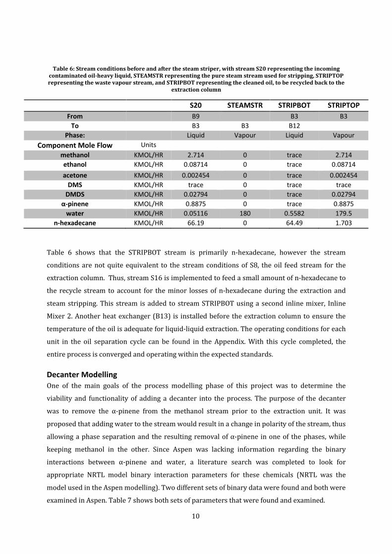
10

Table 6: Stream conditions before and after the steam striper, with stream S20 representing the incoming contaminated oil-heavy liquid, STEAMSTR representing the pure steam stream used for stripping, STRIPTOP representing the waste vapour stream, and STRIPBOT representing the cleaned oil, to be recycled back to the

extraction column

S20 STEAMSTR STRIPBOT STRIPTOP From B9 B3 B3

To B3 B3 B12 Phase: Liquid Vapour Liquid Vapour

Component Mole Flow Units methanol KMOL/HR 2.714 0 trace 2.714 ethanol KMOL/HR 0.08714 0 trace 0.08714 acetone KMOL/HR 0.002454 0 trace 0.002454

DMS KMOL/HR trace 0 trace trace DMDS KMOL/HR 0.02794 0 trace 0.02794

α-pinene KMOL/HR 0.8875 0 trace 0.8875 water KMOL/HR 0.05116 180 0.5582 179.5

n-hexadecane KMOL/HR 66.19 0 64.49 1.703

Table 6 shows that the STRIPBOT stream is primarily n-hexadecane, however the stream

conditions are not quite equivalent to the stream conditions of S8, the oil feed stream for the

extraction column. Thus, stream S16 is implemented to feed a small amount of n-hexadecane to

the recycle stream to account for the minor losses of n-hexadecane during the extraction and

steam stripping. This stream is added to stream STRIPBOT using a second inline mixer, Inline

Mixer 2. Another heat exchanger (B13) is installed before the extraction column to ensure the

temperature of the oil is adequate for liquid-liquid extraction. The operating conditions for each

unit in the oil separation cycle can be found in the Appendix. With this cycle completed, the

entire process is converged and operating within the expected standards.

Decanter Modelling One of the main goals of the process modelling phase of this project was to determine the

viability and functionality of adding a decanter into the process. The purpose of the decanter

was to remove the α-pinene from the methanol stream prior to the extraction unit. It was

proposed that adding water to the stream would result in a change in polarity of the stream, thus

allowing a phase separation and the resulting removal of α-pinene in one of the phases, while

keeping methanol in the other. Since Aspen was lacking information regarding the binary

interactions between α-pinene and water, a literature search was completed to look for

appropriate NRTL model binary interaction parameters for these chemicals (NRTL was the

model used in the Aspen modelling). Two different sets of binary data were found and both were

examined in Aspen. Table 7 shows both sets of parameters that were found and examined.

11

Table 7: NRTL model binary parameters for α-pinene (1) and water (2). The first set of data is extracted from a paper on liquid-liquid equilibrium for binary mixtures (Utami, Sutijan, Roto, & Sediawan, Liquid-Liquid Equilibrium for the Binary Mixtures of Alpha-Pinene+Water+Alpha-Terpineol+Water, 2013). The second set of data is extracted from a paper on liquid-liquid equilibrium for three component systems (Utami, Sutijan, Roto, & Sediawan, Liquid-Liquid Equilibrium for System Composed of Alpha-Pinene, Alpha-Terpineol and Water, 2013).

Parameters Data Set 1 Data Set 2

Bij (J/mol) -5.851e-007 5652.49

Bji (J/mol) 5752.89 7305.75

It was found that the difference between using the first set of parameters and the second set was

minimal. Both produced a ternary diagram for water, methanol and α-pinene that looked like the

one presented in Figure 4.

Figure 4: Ternary plot for a mixture of water, methanol and α-pinene.

Careful consideration of the ternary diagram led to the conclusion that the mole fractions of α-

pinene and water had to be increased in order to achieve separation. Water was added to the

stream and a small separation was eventually achieved. Unfortunately this separation split the

α-pinene in a way that half went into each exiting stream. This result seemed useless as the

extraction column still had to remove a good amount of α-pinene afterwards. In order to justify

12

adding an entire new unit into the process, the team needed better separation results. To

achieve a meaningful separation however, the mole fractions of the water and α-pinene had to

be increased to almost 0.5 each. This would cause the stream to land in the upper area of the

ternary diagram where one of the exiting streams contains virtually all of the α-pinene and the

other contains virtually none. After a series of trial and error optimization steps, it was

determined that an incredibly large amount of water and α-pinene had to be added to dilute the

stream to the desired concentrations (almost 5000 kg/hour of each chemical had to be added).

Even after the separation was achieved, the small amount of residual α-pinene in the methanol

stream was almost equal to the amount that was initially in the stream before adding the

chemicals. It was quite obvious that this was not a viable solution – the cost of the distillation

towers later in the process would be astronomical to separate the water from the methanol.

Furthermore, even if the α-pinene was recycled, further units would be needed to purify the α-

pinene and mix it back into the methanol stream.

The team also examined the separation quality at different temperatures within the decanter. By

reducing the temperature of the stream entering the decanter, better separations were generally

achieved. Unfortunately, changing the temperature within the decanter still did not have a great

enough impact to achieve a satisfactory separation.

With the issues mentioned above regarding the implementation of the decanter, coupled with

the fact that the extraction unit was able to remove virtually all of the α-pinene from the

methanol stream, the team decided that the decanter was simply not a logical or practical option

for this process. No further research was put towards implementing the decanter and the team

focused instead on optimizing the rest of the process.

Process Alternatives Chemrec, a Swedish company focused on optimizing existing pulp and paper plants, has

proposed an alternative process to the one proposed in this report. In their process, waste black

liquor is fed into a high temperature gasification unit along with oxygen (COWI, n.d.). This unit

removes water and some undesirable components from the waste black liquor, resulting in

outlet streams of superheated steam, waste green liquor, and strong black liquor (COWI, n.d.).

The strong black liquor is then passed through a carbon filter in order to remove tars and other

undesirable free carbon. This filter must be initially heated to 1260°C to activate the carbon,

which is very energy intensive (COWI, n.d.).

From the carbon filter, the stream of black liquor passes through a sour shift unit. In this unit,

the product synthesis gas composition is optimized through the catalytic reaction of CO and CO2

13

in the black liquor to form methanol (COWI, n.d.). This process is also fairly energy intensive, as

the catalyst most commonly used is only active in a temperature range of 200°C-500°C (COWI,

n.d.). Once this is finished the stream is fed into an acid gas removal unit. This unit uses solvents

such as C16 under high pressure to remove any sulfur compounds and CO2 present (COWI, n.d.).

The final step in the process involves distillation columns. Two columns are used in series to

remove the remaining water and waste products from the bottoms streams and collect purified

methanol off the top streams (COWI, n.d.).

The Chemrec process appears to work well, but its major disadvantage is that it is very energy

intensive, requiring operation at either high temperatures or high pressure in most parts of the

process. This process is also designed for a much larger scale operation than is being dealt with

in this report. Chemrec installations can process up to 4000 tons per day of black liquor, while

the proposed process handles only about 10 tons per day (COWI, n.d.). This process clearly lies

outside of the scope of the project.

Materials and Equipment Sizing

With a process flow and order selected, the next step is to dimension the individual process

components. This is necessary to ensure proper functionality of the plant, and to allow for cost

estimations of the plant in future sections. In this section, dimensions for each unit operation are

calculated.

Distillation Column Sizing The main design parameters that affect the cost of the two distillation columns are height, inside

diameter, number of trays, and operating pressure (Vasudevan & Ulrich, 2000). The Aspen

simulations automatically calculated the number of trays and operating pressure, while the

height and diameter were calculated using industrial sizing equations. Equation 1 is used to

estimate the height of a distillation column.

𝐻𝑐 = 𝑁𝑡 ∗ 𝑡 (1)

In Equation 1, Nt refers to the number of trays in the column, 𝑡 refers to the tray spacing, and Hc

refers to the height of the column. Aspen modeling provided the appropriate number of trays,

and industry rules of thumb were used for tray spacing (Separation Technology, 2012), allowing

for the height of the tank to be calculated. The Sample Calculations section shows an example of

the column height calculation.

To calculate the diameter of the distillation tank, a few more steps are required. The diameter of

the tank is calculated based on the flooding characteristics and rules of thumb. The column

14

diameter must be kept high enough relative to the vapour velocity within the column to prevent

flooding (Price, 2003). Also, the height to diameter ratio of the tank should never exceed 30 and

is ideally kept below 20 (Price, 2003). The tank diameter was first calculated based on flooding

characteristics, and then checked against the rules of thumb to ensure the height to diameter

requirement was met. Calculations were done for the distillation column to operate at a vapour

velocity of 85% of the flooding capacity. Equation 2 shows how the vapour velocity was

calculated (Hoogstraten & Dunn, 1998).

𝑢𝑓 = 𝐾𝑙�𝜌𝑙−𝜌𝑣𝜌𝑣

(2)

In Equation 2, 𝑢𝑓 refers to the vapour velocity, and 𝜌𝑙 and 𝜌𝑣 refer to the liquid and vapour

densities, respectively. Kl is a constant parameter given in ft/s. The Sample Calculation section

in the Appendix contains exact information on how the vapour velocity was calculated. Given the

design vapour velocity, the cross sectional area of the column was calculated using Equation 3.

𝐴 = 𝑉𝑣0.85𝑢𝑓

(3)

In Equation 3, A refers to the cross sectional area of the column, and Vv refers to the maximum

volumetric flow rate of the vapour (as calculated by Aspen). Once the cross sectional area has

been calculated the radius can be determined. For Sample Calculations, see Appendix.

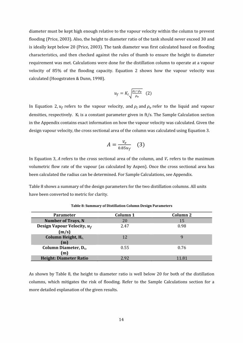
Table 8 shows a summary of the design parameters for the two distillation columns. All units

have been converted to metric for clarity.

Table 8: Summary of Distillation Column Design Parameters

Parameter Column 1 Column 2 Number of Trays, N 20 15

Design Vapour Velocity, 𝒖𝒇 (m/s)

2.47 0.98

Column Height, Hc,

(m) 12 9

Column Diameter, Dc, (m)

0.55 0.76

Height: Diameter Ratio 2.92 11.81

As shown by Table 8, the height to diameter ratio is well below 20 for both of the distillation

columns, which mitigates the risk of flooding. Refer to the Sample Calculations section for a

more detailed explanation of the given results.

15

Extraction Column Sizing

The dimensioning of an extraction column is based on theory concerning mass transfer

coefficients. The type of column chosen to be used and dimensioned has continuous differential

contact, with countercurrent phase flow where one flow is continuous and the other is

dispersed. The industrial column is designed by determining the geometrical dimensions

(diameter and height), which are based on several factors. The column diameter depends on the

processing capacity and the flooding capacity and can be calculated using Equation 4.

𝐷𝑐 = �4 ∗ (𝑄𝑐 + 𝑄𝑑)𝜋 ∗ 𝑘 ∗ 𝐵𝑚𝑚𝑚

(4)

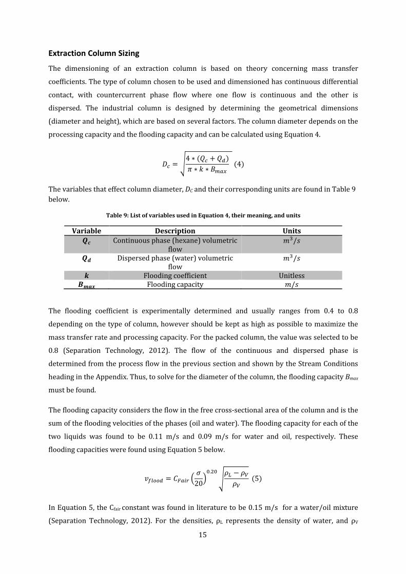
The variables that effect column diameter, DC and their corresponding units are found in Table 9 below.

Table 9: List of variables used in Equation 4, their meaning, and units

Variable Description Units 𝑸𝒄 Continuous phase (hexane) volumetric

flow 𝑚3/𝑠

𝑸𝒅 Dispersed phase (water) volumetric flow

𝑚3/𝑠

𝒌 Flooding coefficient Unitless 𝑩𝒎𝒎𝒎 Flooding capacity 𝑚/𝑠

The flooding coefficient is experimentally determined and usually ranges from 0.4 to 0.8

depending on the type of column, however should be kept as high as possible to maximize the

mass transfer rate and processing capacity. For the packed column, the value was selected to be

0.8 (Separation Technology, 2012). The flow of the continuous and dispersed phase is

determined from the process flow in the previous section and shown by the Stream Conditions

heading in the Appendix. Thus, to solve for the diameter of the column, the flooding capacity Bmax

must be found.

The flooding capacity considers the flow in the free cross-sectional area of the column and is the

sum of the flooding velocities of the phases (oil and water). The flooding capacity for each of the

two liquids was found to be 0.11 m/s and 0.09 m/s for water and oil, respectively. These

flooding capacities were found using Equation 5 below.

𝑣𝑓𝑙𝑓𝑓𝑑 = 𝐶𝐹𝑚𝐹𝐹 �𝜎

20�0.20

�𝜌𝐿 − 𝜌𝑉𝜌𝑉

(5)

In Equation 5, the Cfair constant was found in literature to be 0.15 m/s for a water/oil mixture

(Separation Technology, 2012). For the densities, ρL represents the density of water, and ρV

16

represents the oil density (in kg/m3), which is always less than water. Lastly, σ represents the

surface tension of the phase in question (in dyn/cm). With voil an3d vwater determined, the

diameter of the column can be found using Equation 4.

After substituting all the values in to Equation 4, the column diameter was calculated to be 4 m.

This unit is designed to be vertically oriented with tower packing. The tower packing material

consists of random polymeric and the vessel material is carbon steel. To see exactly how the

numerical results were generated for the extraction column design, refer to the Sample

Calculations section.

Steam Stripper For the purposes of sizing and cost estimation, it was assumed that the design equations for

Distillation Columns could also be applied to steam strippers. This was deemed to be a fair

assumption as steam strippers in industry are sized similarly to distillation columns, where the

height is a function of the number of trays and the diameter is chosen to prevent flooding (KLM

Technology Group, 2011). The diameter of distillation columns is typically chosen so that the

maximum vapour velocity is between 50-80% of the flooding velocity (Redel, Novoa, Goldina, &

Englert, N/A), while the diameter of strippers are chosen so that the vapour velocity is between

60-80% of the flooding velocity (KLM Technology Group, 2011). This assumption was also

deemed to be safe from an economic standpoint, as the Ulrich cost estimation database does not

distinguish between distillation and stripping columns for the purposes of cost estimation. Table

10 summarizes the design parameters calculated for the steam stripper. The Sample

Calculations section shows the specific method of calculation to obtain these results, which

follow an identical method as the distillation column calculations.

Table 10: Summary of Steam Stripper Design Parameters

Parameter Value Number of Trays, N 20

Design Vapour Velocity, 𝒖𝒇 (m/s)

0.35

Column Height, Hc,

(m) 26

Column Diameter, Dc, (m)

2.78

Height : Diameter Ratio 9.35

17

Mixer and Pump For the pump, a power requirement value was generated by Aspen based off the process flow

that the pump could be handling. For the inline mixers, literature values were used to match a

power rating with the flows that the pieces of equipment were likely to handle. Table 11 shows

the mixer and pump results.

Table 11: Determined power requirements for the two inline mixer and the centrifugal pump, based off of Aspen results and the flow being handled (Silverson, 2015)

Equipment Power Requirement (kW)

Inline Mixer 1 1.5 Inline Mixer 2 22.37

Centrifugal Pump 1.51

Heat Exchangers

The design parameters of interest for heat exchangers as far as cost estimation and process

planning are the operating pressure, heat duty, and heat transfer surface area. The Aspen

simulations performed the calculations for the operating pressures and heat duties

automatically, but did not calculate the surface area. The required surface area was calculated

using Equation 6.

𝑄 = 𝑈𝐴Δ𝑇 (6)

In Equation 6, Q refers to the heat duty, U refers to the heat transfer coefficient, A refers to the

surface area of the exchanger, and the ΔT refers to the change in temperature of the product

entering and exiting the heat exchanger. The temperature change and heat duty can be taken

from Aspen simulations, and the heat transfer coefficient can be estimated from tabulated

literature data, assuming the heating fluid to be steam and the product being heated to have heat

transfer characteristics similar to the majority component of the stream. For example, in the first

heat exchanger, where the fluid being heated is mostly n-hexadecane, the heat transfer

coefficient was estimated to be the tabulated coefficient for heat transfer between n-hexadecane

and steam.

Given the heat duty, heat transfer coefficient, and temperature change, the required surface area

was calculated. Table 12 summarizes the design parameters recommended for the heat

exchangers in the process. The simple calculation for surface area is shown in the Sample

Calculation section of the Appendix.

18

Table 12: Summary of Heat Exchanger Design Parameters (Teralba, 2015)

Parameter Exchanger 1 Exchanger 2 Operating Pressure, P

(bar) 1 1

Heat Duty, Q (kW)

1076 1200

Temperature Change, ΔT 108 116

Heat Transfer Coefficient, U (W/m2K)

1000 1000

Surface Area, A (m2)

9.96 10.34

Investment Cost Analysis

Plant Cost

With the operating parameters and dimensions of the plant equipment confirmed, it is possible

to calculate the cost of each unit operation and thus an estimated final cost for the plant

production. The results represent an estimation of the total ‘fixed cost’ involved with this

process. To complete these calculations, the Ulrich method is used, as it is the most

comprehensive with respect to the factors used to arrive at a final cost. The EconExpert program

utilizes the Ulrich method and was the main source of plant cost estimations, based off of inputs

determined in the previous section. For the first distillation column, Table 13 displays the

EconExpert input and the cost results for the first distillation column.

19

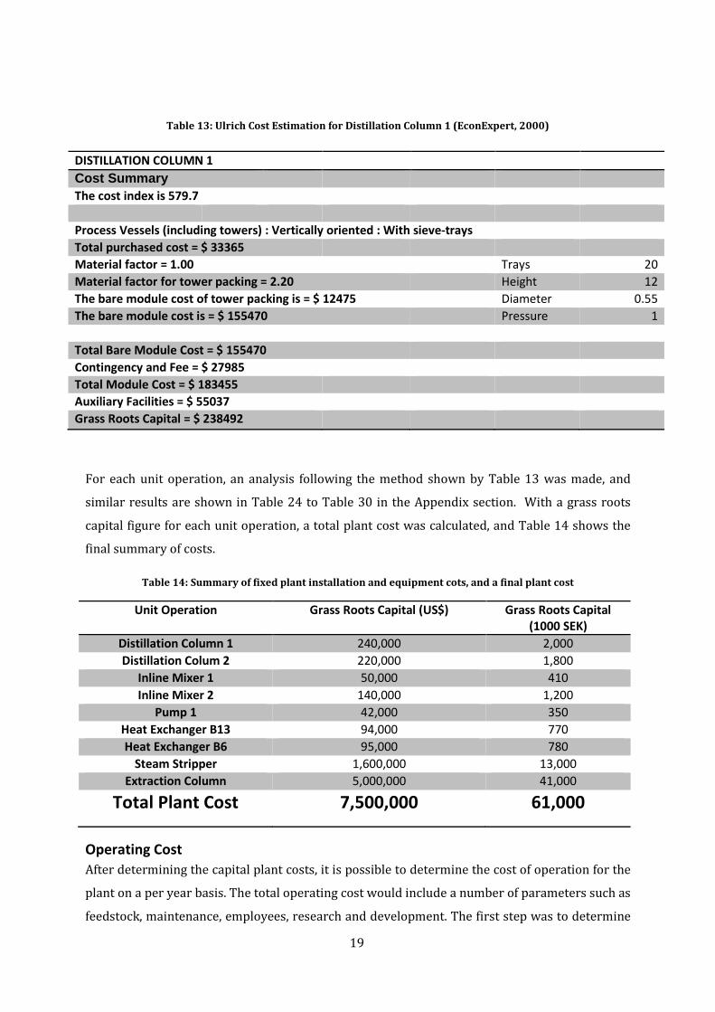
Table 13: Ulrich Cost Estimation for Distillation Column 1 (EconExpert, 2000)

For each unit operation, an analysis following the method shown by Table 13 was made, and

similar results are shown in Table 24 to Table 30 in the Appendix section. With a grass roots

capital figure for each unit operation, a total plant cost was calculated, and Table 14 shows the

final summary of costs.

Table 14: Summary of fixed plant installation and equipment cots, and a final plant cost

Unit Operation Grass Roots Capital (US$) Grass Roots Capital (1000 SEK)

Distillation Column 1 240,000 2,000 Distillation Colum 2 220,000 1,800

Inline Mixer 1 50,000 410 Inline Mixer 2 140,000 1,200

Pump 1 42,000 350 Heat Exchanger B13 94,000 770 Heat Exchanger B6 95,000 780

Steam Stripper 1,600,000 13,000 Extraction Column 5,000,000 41,000

Total Plant Cost 7,500,000 61,000

Operating Cost After determining the capital plant costs, it is possible to determine the cost of operation for the

plant on a per year basis. The total operating cost would include a number of parameters such as

feedstock, maintenance, employees, research and development. The first step was to determine

DISTILLATION COLUMN 1 Cost Summary The cost index is 579.7 Process Vessels (including towers) : Vertically oriented : With sieve-trays Total purchased cost = $ 33365 Material factor = 1.00 Trays 20 Material factor for tower packing = 2.20 Height 12 The bare module cost of tower packing is = $ 12475 Diameter 0.55 The bare module cost is = $ 155470 Pressure 1 Total Bare Module Cost = $ 155470 Contingency and Fee = $ 27985 Total Module Cost = $ 183455 Auxiliary Facilities = $ 55037 Grass Roots Capital = $ 238492

20

the cost of the feedstock, which includes water used for steam and heating oil costs. The cost of

steam was found to be 66 SEK/ton, which equates to 158.4 SEK/day and then multiplied by the

number of days in a year to find the total yearly cost. Similarly, to find the yearly cost of heating

oil, the average cost in US dollars was found, and inflated by multiplying it by 1.5 to account for

error in prices, as Swedish costs were not readily available. Then the actual cost of heating oil

was multiplied by the flow rate of 0.0058 𝑚3/𝑚𝑚𝑚 and converted to costs per year in Swedish

currency. The results of all of these calculations are summarized in Table 15.

Table 15: Average Heating Oil Costs

Type of Cost Value Unit Average Cost 2.69 USD/gal

0.71 USD/L 709.8 USD/𝑚3

Actual Costs 1065 USD/𝑚3 6.199 USD/min

Yearly cost 3,300,000 USD/year 27,000,000 SEK/year

After determining the feedstock operating prices, the maintenance and repair operating cost is

calculated using the rule of thumb given by the project coordinator as a 2-10% of the Grass

Roots Capital cost. For the calculations performed, 6% of the Grass Roots Capital cost was used.

Furthermore the cost of spare parts is calculated as 15% of the maintenance costs. Once the

maintenance costs are determined, the cost of employees of the plant can be found again using

the rule of thumbs provided and wage statistics for Sweden operators (StatsSkuld, 2013). These

costs are summarized below in

Table 16 below.

21

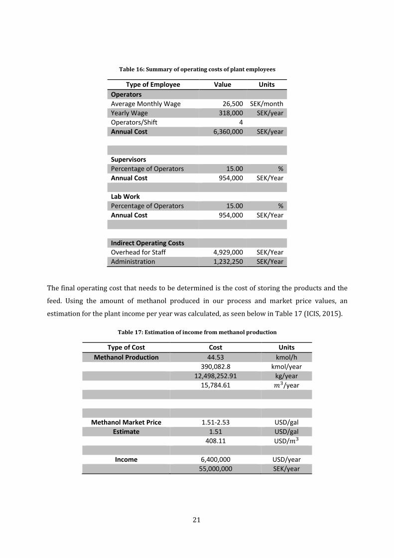
Table 16: Summary of operating costs of plant employees

Type of Employee Value Units Operators Average Monthly Wage 26,500 SEK/month Yearly Wage 318,000 SEK/year Operators/Shift 4 Annual Cost 6,360,000 SEK/year Supervisors Percentage of Operators 15.00 % Annual Cost 954,000 SEK/Year Lab Work Percentage of Operators 15.00 % Annual Cost 954,000 SEK/Year Indirect Operating Costs Overhead for Staff 4,929,000 SEK/Year Administration 1,232,250 SEK/Year

The final operating cost that needs to be determined is the cost of storing the products and the

feed. Using the amount of methanol produced in our process and market price values, an

estimation for the plant income per year was calculated, as seen below in Table 17 (ICIS, 2015).

Table 17: Estimation of income from methanol production

Type of Cost Cost Units Methanol Production 44.53 kmol/h

390,082.8 kmol/year 12,498,252.91 kg/year 15,784.61 𝑚3/year

Methanol Market Price 1.51-2.53 USD/gal Estimate 1.51 USD/gal

408.11 USD/𝑚3

Income 6,400,000 USD/year 55,000,000 SEK/year

22

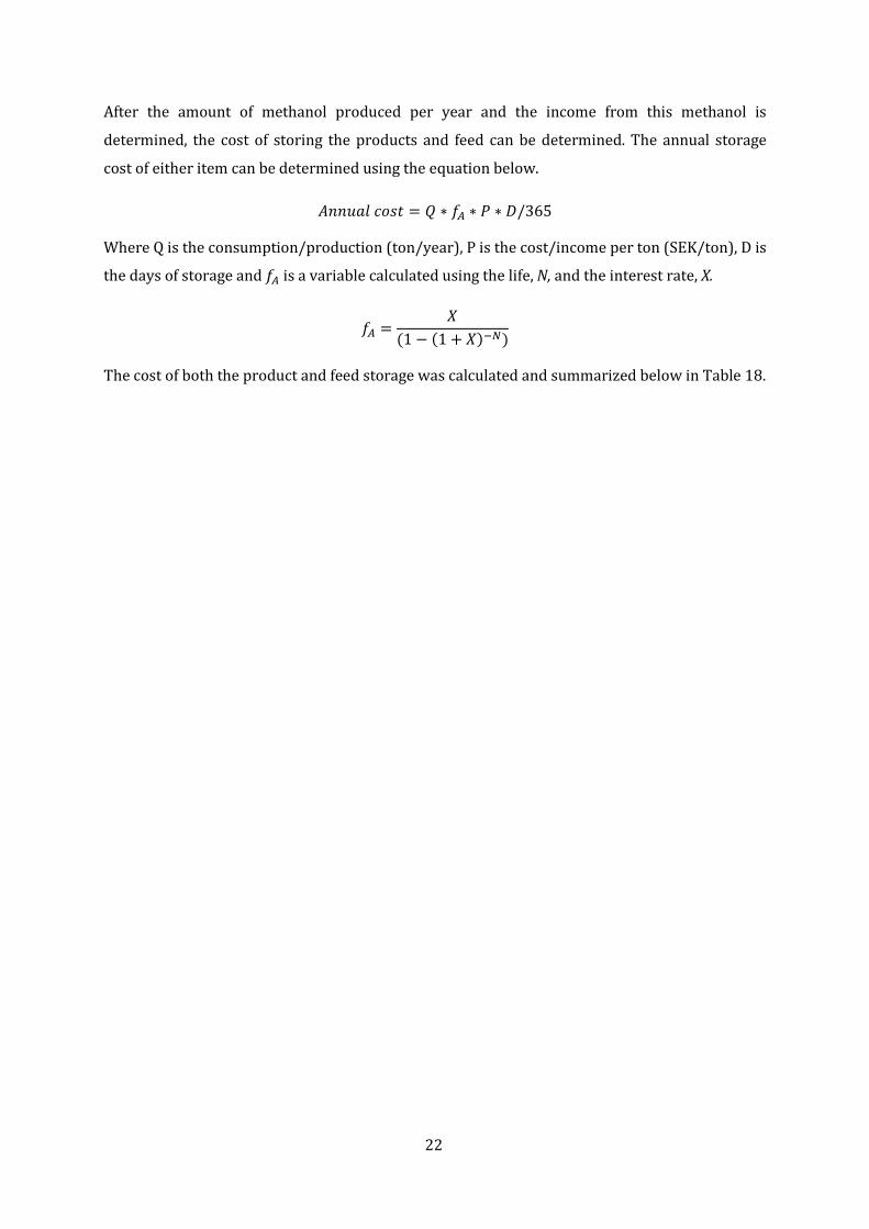
After the amount of methanol produced per year and the income from this methanol is

determined, the cost of storing the products and feed can be determined. The annual storage

cost of either item can be determined using the equation below.

𝐴𝑚𝑚𝑢𝐴𝐴 𝑐𝑐𝑠𝑡 = 𝑄 ∗ 𝑓𝐴 ∗ 𝑃 ∗ 𝐷/365

Where Q is the consumption/production (ton/year), P is the cost/income per ton (SEK/ton), D is

the days of storage and 𝑓𝐴 is a variable calculated using the life, N, and the interest rate, X.

𝑓𝐴 =𝑋

(1 − (1 + 𝑋)−𝑁)

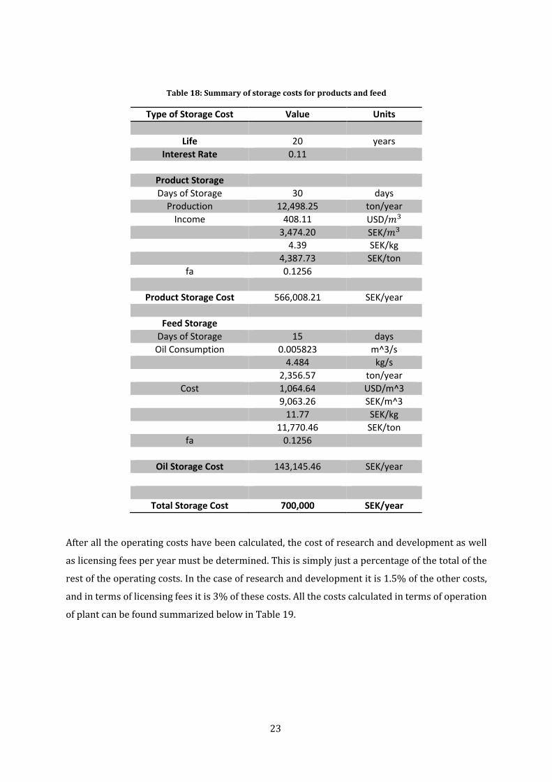
The cost of both the product and feed storage was calculated and summarized below in Table 18.

23

Table 18: Summary of storage costs for products and feed

Type of Storage Cost Value Units

Life 20 years Interest Rate 0.11

Product Storage Days of Storage 30 days

Production 12,498.25 ton/year Income 408.11 USD/𝑚3

3,474.20 SEK/𝑚3 4.39 SEK/kg 4,387.73 SEK/ton

fa 0.1256

Product Storage Cost 566,008.21 SEK/year

Feed Storage Days of Storage 15 days

Oil Consumption 0.005823 m^3/s 4.484 kg/s 2,356.57 ton/year

Cost 1,064.64 USD/m^3 9,063.26 SEK/m^3 11.77 SEK/kg 11,770.46 SEK/ton

fa 0.1256

Oil Storage Cost 143,145.46 SEK/year

Total Storage Cost 700,000 SEK/year

After all the operating costs have been calculated, the cost of research and development as well

as licensing fees per year must be determined. This is simply just a percentage of the total of the

rest of the operating costs. In the case of research and development it is 1.5% of the other costs,

and in terms of licensing fees it is 3% of these costs. All the costs calculated in terms of operation

of plant can be found summarized below in Table 19.

24

Table 19: Total annual operating costs for the plant

Type of Cost Cost (SEK) Feedstock

Water 58,000 Oil 28,000,000

Maintenance 3,800,000 Spare Parts 570,000 Operators 6,400,000 Supervisors 950,000 Lab Work 950,000 Storage Costs 710,000 Research and Development 620,000 Licensing Fees 1,200,000 Total Operating Cost 43,000,000

Thus, the total plant operating cost is 43,010,647 SEK/year or 5,125,643.32 USD/year.

Sensitivity Analysis and Feasibility Study The main factors affecting the Net Present Value (NPV) for this project could be divided into

three categories: those affecting the Grassroots Capital cost, those affecting the operating costs,

and those affecting the income. The initial list of factors affecting the cost can be found in Table

33 of the Appendix.

The main factors affecting Grassroots capital investment had to do with the sizing and design

parameters of the unit operations in the process. Naturally there were some parameters that

could not be adjusted, as doing so would prevent the process from achieving the desired

performance. It was found, however, that the tray spacing could be adjusted without reducing

the performance of the process, and that doing so would affect the size and cost of the

distillation columns.

The other main sources of uncertainty were in the operating costs and income estimates. The

cost of extraction oil had a range of possible values. Also, the sale value of the final methanol

product and the interest rate over the product’s lifetime were uncertain. Many other operating

costs were calculated by industry rules of thumb provided by the project supervisor. These rules

of thumb came with inherent uncertainty, and as a result also affected the NPV. Table 20 shows

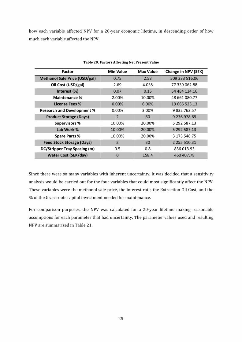
25

how each variable affected NPV for a 20-year economic lifetime, in descending order of how

much each variable affected the NPV.

Table 20: Factors Affecting Net Present Value

Factor Min Value Max Value Change in NPV (SEK) Methanol Sale Price (USD/gal) 0.75 2.53 509 233 516.06

Oil Cost (USD/gal) 2.69 4.035 77 339 062.88 Interest (%) 0.07 0.15 54 484 124.16

Maintenance % 2.00% 10.00% 48 661 080.77 License Fees % 0.00% 6.00% 19 665 525.13

Research and Development % 0.00% 3.00% 9 832 762.57 Product Storage (Days) 2 60 9 236 978.69

Supervisors % 10.00% 20.00% 5 292 587.13 Lab Work % 10.00% 20.00% 5 292 587.13

Spare Parts % 10.00% 20.00% 3 173 548.75 Feed Stock Storage (Days) 2 30 2 255 510.31

DC/Stripper Tray Spacing (m) 0.5 0.8 836 013.93 Water Cost (SEK/day) 0 158.4 460 407.78

Since there were so many variables with inherent uncertainty, it was decided that a sensitivity

analysis would be carried out for the four variables that could most significantly affect the NPV.

These variables were the methanol sale price, the interest rate, the Extraction Oil Cost, and the

% of the Grassroots capital investment needed for maintenance.

For comparison purposes, the NPV was calculated for a 20-year lifetime making reasonable

assumptions for each parameter that had uncertainty. The parameter values used and resulting

NPV are summarized in Table 21.

26

Table 21: Summary of Reference NPV Conditions

Parameter Value Methanol Sale Price

(USD/gal) 1.51

Interest (%) 0.11 Oil Cost (USD/gal) 4.035

DC/Stripper Tray Spacing (m) 0.6 Water Cost (SEK/day) 158.4

Maintenance % 6.00% Spare Parts % 15.00% Supervisors % 15.00%

Lab Work % 15.00% License Fees % 3.00%

Research and Development %

1.50%

FeedStock Storage (Days) 15 Product Storage (Days) 30

NPV (SEK) 31 000 000

The following sections break down how the minimum and maximum values were determined

for each parameter, and take a more in depth look at how each factor affects the NPV. Under

reference conditions, the NPV after the 20 year economic lifetime of the project was calculated

to be 30 632 598.64 SEK, and the payoff time was calculated to be 9 years. See appendix for

sample calculations and Appendix Table 32 for a summary of NPV and pay off time calculations.

Methanol Sale Price As shown in Table 21, the most significant factor affecting the NPV of the project was the price at

which the green methanol product could be sold. This makes sense as the only source of income

for the project comes from sales of the methanol product. A typical range for bulk methanol sales

was found to be $1.51-$2.53 US/gal (ICIS, 2006), depending on the purity. In a worst-case

scenario, the produced methanol could not be sold at or near industry standard prices. It was

therefore assumed that the minimum possible sale value for the produced methanol would be

half of the lowest market price, giving the minimum sale value of $0.75 US/gal. In the unlikely

case that the produced methanol could be sold at the highest possible market value, the

methanol could be sold at $2.53 US/gal. This value was therefore used as the upper limit for the

sensitivity analysis. It was assumed that in reality, a growing demand for biofuels over the next

20 years would allow the produced methanol to be sold at or near industry standard prices. For

this reason, the reference NPV was calculated for a methanol-selling price of $1.51 US/gal.

27

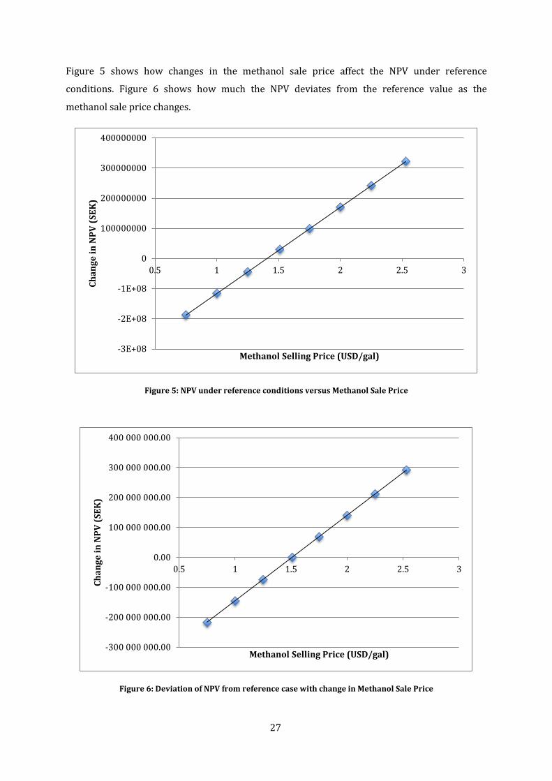
Figure 5 shows how changes in the methanol sale price affect the NPV under reference

conditions. Figure 6 shows how much the NPV deviates from the reference value as the

methanol sale price changes.

Figure 5: NPV under reference conditions versus Methanol Sale Price

Figure 6: Deviation of NPV from reference case with change in Methanol Sale Price

-3E+08

-2E+08

-1E+08

0

100000000

200000000

300000000

400000000

0.5 1 1.5 2 2.5 3

Chan

ge in

NPV

(SEK

)

Methanol Selling Price (USD/gal)

-300 000 000.00

-200 000 000.00

-100 000 000.00

0.00

100 000 000.00

200 000 000.00

300 000 000.00

400 000 000.00

0.5 1 1.5 2 2.5 3

Chan

ge in

NPV

(SEK

)

Methanol Selling Price (USD/gal)

28

As seen in Figures 5 and 6, the methanol selling price has the potential to single handedly

determine whether or not this project is economically viable. Under reference conditions for all

other parameters, the venture becomes unprofitable if the methanol is sold for any less than

about $1.40 US/gal. It should also be mentioned that the actual sale price of the methanol is

more likely to fall short of the reference assumption of $1.51 US/gal than to exceed it, at least in

the initial years of the project. This is because the purity of the product is not quite at industry

standard, and at this point biofuels are not generally as valuable as conventional fuels. If the

selling price drops from the predicted $1.51 US/gal by just 11 cents to $1.40 US/gal, the project

will only break even after the 20-year economic lifetime. This makes the selling price of

methanol a highly sensitive parameter when evaluating the feasibility of this project. The true

selling price must be further examined to eliminate uncertainty before it can be conclusively

determined whether the project will be feasible or not.

Extraction Oil Price

The price of oil used in the extraction column in the process was found to be the second most

significant source of uncertainty. The exact solvent used in the Aspen model was n-hexadecane,

which does not have bulk pricing information readily available. As a result, the cost of the oil was

estimated using the price of standard heating oil. The base price for this oil is $2.69 US/gal (US

Energy Information Administration, 2015). Since n-hexadecane is a more specific product and

would likely cost more, this price was used as the minimum possible oil cost. The maximum

possible value was given by the project supervisor to be 50% more than the cost of heating oil,

which comes to $4.04 US/gal. With no true indication of where in this range the actual price of

oil would fall, the reference value for oil price was chosen as the maximum $4.04 US/gal.

Figure 7 shows how changes in the oil price affect the NPV under reference conditions. Figure 8

shows how much the NPV deviates from the reference value as the oil price changes.

29

Figure 7: NPV under reference conditions versus extraction oil price

Figure 8: Deviation of NPV from reference conditions versus extraction oil price

Since the reference value was selected as the maximum possible oil price, any departure from

the reference value was associated with an increase in the NPV, as shown in Figures 7 and 8. The

NPV increases as the cost of oil decreases, up to the minimum possible oil price of $2.69 US/gal,

which results in an increase in NPV of about 78 million SEK after 20 years. This would

0

20000000

40000000

60000000

80000000

100000000

120000000

2.6 2.8 3 3.2 3.4 3.6 3.8 4 4.2

NPV

(SEK

)

Oil Price (USD/gal)

0.00

10 000 000.00

20 000 000.00

30 000 000.00

40 000 000.00

50 000 000.00

60 000 000.00

70 000 000.00

80 000 000.00

90 000 000.00

2.5 2.7 2.9 3.1 3.3 3.5 3.7 3.9 4.1 4.3

NPV

(SEK

)

Oil Price (USD/gal)

30

correspond to an increase of about 254.6% on the reference NPV. This would be a huge boost to

the feasibility of the project, and would allow more room for error in the product selling price,

interest rate, and maintenance cost estimations.

It has therefore been concluded that the oil price has good potential to increase the profitability

of the project. Any measures should be taken to reduce the cost of purchasing extraction oil, as

doing so will significantly improve the project economics. It does, however, remain uncertain

how much the oil will cost. For this reason all estimations should assume the maximum possible

oil price.

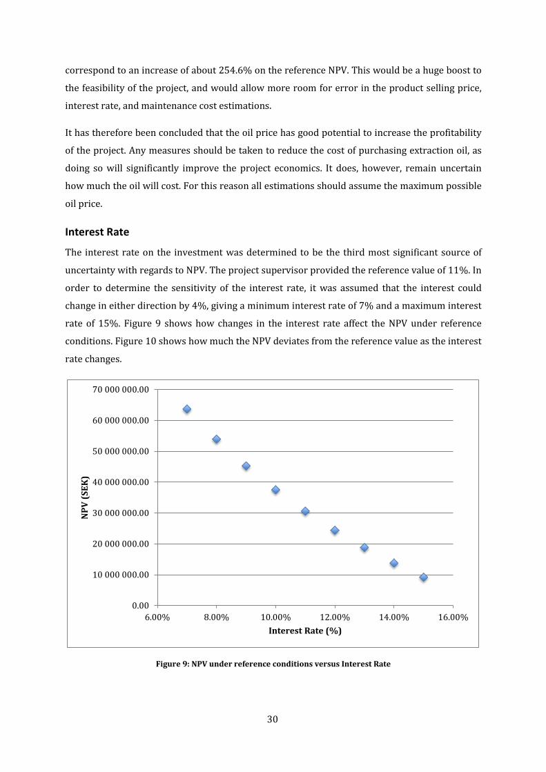
Interest Rate

The interest rate on the investment was determined to be the third most significant source of

uncertainty with regards to NPV. The project supervisor provided the reference value of 11%. In

order to determine the sensitivity of the interest rate, it was assumed that the interest could

change in either direction by 4%, giving a minimum interest rate of 7% and a maximum interest

rate of 15%. Figure 9 shows how changes in the interest rate affect the NPV under reference

conditions. Figure 10 shows how much the NPV deviates from the reference value as the interest

rate changes.

Figure 9: NPV under reference conditions versus Interest Rate

0.00

10 000 000.00

20 000 000.00

30 000 000.00

40 000 000.00

50 000 000.00

60 000 000.00

70 000 000.00

6.00% 8.00% 10.00% 12.00% 14.00% 16.00%

NPV

(SEK

)

Interest Rate (%)

31

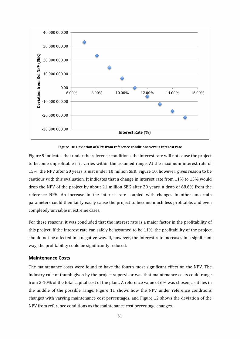
Figure 10: Deviation of NPV from reference conditions versus interest rate

Figure 9 indicates that under the reference conditions, the interest rate will not cause the project

to become unprofitable if it varies within the assumed range. At the maximum interest rate of

15%, the NPV after 20 years is just under 10 million SEK. Figure 10, however, gives reason to be

cautious with this evaluation. It indicates that a change in interest rate from 11% to 15% would

drop the NPV of the project by about 21 million SEK after 20 years, a drop of 68.6% from the

reference NPV. An increase in the interest rate coupled with changes in other uncertain

parameters could then fairly easily cause the project to become much less profitable, and even

completely unviable in extreme cases.

For these reasons, it was concluded that the interest rate is a major factor in the profitability of

this project. If the interest rate can safely be assumed to be 11%, the profitability of the project

should not be affected in a negative way. If, however, the interest rate increases in a significant

way, the profitability could be significantly reduced.

Maintenance Costs

The maintenance costs were found to have the fourth most significant effect on the NPV. The

industry rule of thumb given by the project supervisor was that maintenance costs could range

from 2-10% of the total capital cost of the plant. A reference value of 6% was chosen, as it lies in

the middle of the possible range. Figure 11 shows how the NPV under reference conditions

changes with varying maintenance cost percentages, and Figure 12 shows the deviation of the

NPV from reference conditions as the maintenance cost percentage changes.

-30 000 000.00

-20 000 000.00

-10 000 000.00

0.00

10 000 000.00

20 000 000.00

30 000 000.00

40 000 000.00

6.00% 8.00% 10.00% 12.00% 14.00% 16.00%

Dev

iati

on fr

om R

ef N

PV (S

EK)

Interest Rate (%)

32

Figure 11: NPV under reference conditions versus Maintenance Cost %

Figure 12: Deviation of NPV from reference value versus Maintenance Cost %

Figure 11 shows that maintenance costs on the high end of the expected range will not cause the

project to become unprofitable on their own. However, higher than expected maintenance costs

could easily couple with unfavorable values for other uncertain variables to eliminate the

economic viability of this project. An increase of the maintenance costs from 6% to 10% of the

initial capital investment would reduce the NPV by about 24 million SEK over 20 years, a

0

10000000

20000000

30000000

40000000

50000000

60000000

0.00% 2.00% 4.00% 6.00% 8.00% 10.00% 12.00%

NPV

(SEK

)

Maintenance Cost (%)

-30 000 000.00

-20 000 000.00

-10 000 000.00

0.00

10 000 000.00

20 000 000.00

30 000 000.00

0.00% 2.00% 4.00% 6.00% 8.00% 10.00% 12.00%

Dev

iati

on fr

om R

ef N

PV (S

EK)

Maintenance Cost (%)

33

reduction of 78.3%. This reduction is significant, and could couple with an increase in the

interest rate or a decrease in the methanol sale price to render the project unprofitable.

In summary, there exists too much uncertainty in the values of methanol sale price, extraction

oil price, interest rate, and maintenance costs to accurately predict whether this process would

be economically feasible. An unfavorable deviation in any of the methanol price, oil price, or

interest rate over the 20 year economic lifetime of this project could severely reduce the

economic viability of this project. It is recommended that a higher level of certainty be attained

for all these variables before proceeding with the project.

Conclusions and Recommendations After conducting extensive research on the kraft pulping process, a process was designed to

create a green methanol biofuel from the kraft pulping process effluent. The requirement for this

biofuel is that the water content is less than 0.1%, by mass, and the concentration of sulfur-

containing compounds is less than 10 ppm. To achieve this, a process was created with two main

functions: a methanol refinement system, and an oil cleaning system. The methanol refinement

system consists of two distillation columns, an inline mixer, and an extraction column. After

modeling the refinement system with Aspen, it was determined that a combined

methanol/ethanol purity in the final stream is above 99% by mass. In addition, the mass fraction

of sulphur containing compounds (DMS and DMDS) is 3.32x10-7, which is below the industrial

regulations, and the water content is 0.7%. It is observed that the water content requirement is

not met; however, it is suspected that a small amount of further fine tuning of the second

distillation column in the process will achieve the desired concentration. It is therefore

recommended that further research goes into altering the operating conditions and parameters

of this column to see if the water content requirement can be met. To improve the cost efficiency

of the process, an oil cleaning system was added to the process, which allows the oil required for

the extraction column to be reused. This oil cleaning system consists primarily of a steam

stripper, but also includes a heat exchanger, a pump, and an inline mixer.

It should be noted that the proposed process demands a very large supply of extraction oil. In

the tuning and optimization stages of the process design, the main goal was to produce methanol

at as high purity as possible. Since using more extraction oil resulted in a more purified

methanol product stream, extraction oil was added with little regard to the potential economic

consequences. After the economic calculations were carried out, it became clear that the oil was

added to the point of diminishing returns with respect to methanol purity. More specifically, the

high oil demand results in greater loss of oil, a larger steam stripper, and a larger extraction

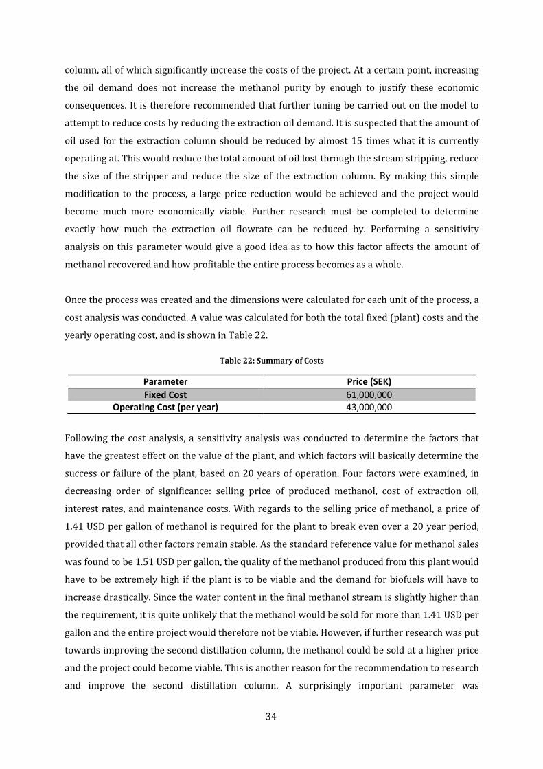
34

column, all of which significantly increase the costs of the project. At a certain point, increasing

the oil demand does not increase the methanol purity by enough to justify these economic

consequences. It is therefore recommended that further tuning be carried out on the model to

attempt to reduce costs by reducing the extraction oil demand. It is suspected that the amount of

oil used for the extraction column should be reduced by almost 15 times what it is currently

operating at. This would reduce the total amount of oil lost through the stream stripping, reduce

the size of the stripper and reduce the size of the extraction column. By making this simple

modification to the process, a large price reduction would be achieved and the project would

become much more economically viable. Further research must be completed to determine

exactly how much the extraction oil flowrate can be reduced by. Performing a sensitivity

analysis on this parameter would give a good idea as to how this factor affects the amount of

methanol recovered and how profitable the entire process becomes as a whole.

Once the process was created and the dimensions were calculated for each unit of the process, a

cost analysis was conducted. A value was calculated for both the total fixed (plant) costs and the

yearly operating cost, and is shown in Table 22.

Table 22: Summary of Costs

Parameter Price (SEK) Fixed Cost 61,000,000

Operating Cost (per year) 43,000,000

Following the cost analysis, a sensitivity analysis was conducted to determine the factors that

have the greatest effect on the value of the plant, and which factors will basically determine the

success or failure of the plant, based on 20 years of operation. Four factors were examined, in

decreasing order of significance: selling price of produced methanol, cost of extraction oil,

interest rates, and maintenance costs. With regards to the selling price of methanol, a price of

1.41 USD per gallon of methanol is required for the plant to break even over a 20 year period,

provided that all other factors remain stable. As the standard reference value for methanol sales

was found to be 1.51 USD per gallon, the quality of the methanol produced from this plant would

have to be extremely high if the plant is to be viable and the demand for biofuels will have to

increase drastically. Since the water content in the final methanol stream is slightly higher than

the requirement, it is quite unlikely that the methanol would be sold for more than 1.41 USD per

gallon and the entire project would therefore not be viable. However, if further research was put

towards improving the second distillation column, the methanol could be sold at a higher price

and the project could become viable. This is another reason for the recommendation to research

and improve the second distillation column. A surprisingly important parameter was

35

determined to be the cost of extraction oil. Likely because of the oil-cleaning system and the

reuse of extraction oil, if a cheap oil price is found (approx. 2.60 USD per gallon), it has the

potential to boost the economic efficiency of this project significantly, potentially offsetting

losses due to low methanol selling price. With regards to maintenance costs and interest rate, it

was determined that with an interest rate of 11% (which is expected) the profitability of the

project would not be affected too heavily, however it should not exceed 13%. Lastly, if a

maintenance cost of 6% of the plant capital cost was maintained, the cost impact is rather low in

the grand scheme of the project, and there is about 4% leeway until the maintenance cost

becomes a significant threat.

After concluding this project, four major recommendations have been revealed. The most

important recommendation is that more research needs to be made to find more exact pricing

for the operating variables, such as material costs and the selling price of methanol. Both of

these factors, as proven in the sensitivity analysis, have enough of an impact on the value of the

plant to make it extremely viable or not viable whatsoever. Thus, an exact price value must be

determined for these factors. Secondly, it is recommended that further research goes into

optimizing the second distillation column to reach the water content requirements for the final

methanol stream. The type of trays should be examined along with the number of trays to see if

the column can be finely tuned to achieve the desired purity. Other operating parameters should

be examined as well. If the water content was reduced adequately, the methanol stream could

perhaps be sold at a high enough price to make the project economically feasible. Finally, it was

noted that water and steam costs are a significant expense with regards to this operation. Two

recommendations for future examination would be the addition of a water-cleaning system for

stream S12, the bottoms of the final methanol distillation column, and a water/steam cleaning

system for the STRIPTOP stream, which is the top stream from the steam stripper. Cleaning

these streams, which contain primarily water and steam, would allow the reuse of water and

steam and could incur significant cost reductions to the project.

36

Bibliography COWI. (n.d.). Black Liquorto Methanol or DME. Retrieved from CHEMREC:

http://www.cowi.se/menu/projekt/Industri-och-Energi/Documents/Black%20Liquor%20to%20Methanol%20or%20DME%20Chemrec.pdf

EconExpert. (2000). UlrichDesign. Retrieved 2015, from http://www.ulrichvasudesign.com/econ.html

European Paper & Packaging Industries. (2015). Types of Pulping Processes. Retrieved 2015, from Paper Online: http://www.paperonline.org/paper-making/paper-production/pulping/types-of-pulping-processes

Exchange-Rates. (2015). Swedish Kronor (SEK) to US Dollar (USD). Retrieved 2015, from Exchange-Rates: http://www.exchange-rates.org/Rate/SEK/USD/1-3-2014

Hoogstraten, C., & Dunn, K. (1998). Separation Processes. Retrieved 2015, from McMaster University: http://learnche.mcmaster.ca/wiki_4M3/images/c/c7/Distillation-project-report-vanHoogstraten-Dunn-UCT-1998.pdf

ICIS. (2006, August 28). Indicative Chemical Prices A-Z. Retrieved May 20, 2015, from http://www.icis.com/chemicals/channel-info-chemicals-a-z/

ICIS. (2015). Indicative Chemical Prices A-Z. Retrieved 2015, from ICIS: http://www.icis.com/chemicals/channel-info-chemicals-a-z/

KLM Technology Group. (2011). Distillation Column Selection and Sizing. Retrieved 2015, from KLM Technology Group: http://kolmetz.com/pdf/EDG/ENGINEERING%20DESIGN%20GUIDELINES%20-%20distillation%20column%20-%20Rev%2004%20web.pdf

Koncseg, C., & Barbulescu, A. (2011). Liquid-Liquid Extraction With and Without a Chemical Reaction. Retrieved 2015, from InTech: http://cdn.intechopen.com/pdfs-wm/13535.pdf

Price, R. (2003). Distillation. Retrieved 2015, from http://facstaff.cbu.edu/rprice/lectures/distill7.html

Redel, M., Novoa, A., Goldina, T., & Englert, M. (N/A). Distillation. Retrieved 2015, from University of Utah: http://www.che.utah.edu/~ring/Design%20I/Articles/distillation%20design.pdf

Separation Technology. (2012). Distillation Column Tray Selection & Sizing. Retrieved 2015, from Separation Technologies: http://seperationtechnology.com/distillation-column-tray-selection-1/

Sigma Aldrich. (2014). Benzaldehyde. Retrieved Febrary 24, 2014, from http://www.sigmaaldrich.com/catalog/product/aldrich/w212717?lang=en&region=CA

Silverson. (2015). High Shear In-Line Mixers - Technical Information. Retrieved 2015, from Silverson: http://www.silverson.com/us/products/in-line-mixers/technical-information

37

StatsSkuld. (2013). The Statistical wage for Wood chip plant operators, forestry in Sweden. Retrieved 2015, from StatsSkuld: http://en-sv.statsskuld.se/salary/for-Wood+chip+plant+operators%2C+forestry-158027/2013/

Steltenkamp, M. S. (1985, March 26). Patent No. US4507172 A.

Teralba. (2015). Mixing and Agitating Solutions. Retrieved 2015, from Teralba: http://www.teralba.com/heat-exchangers/mixers-and-agitators-solutions

Thermopedia. (2011). Heat Transfer Coefficient. Retrieved 2015, from Thermopedia: http://www.thermopedia.com/content/841/

US Energy Information Administration. (2015, April 1). Petroleum and Other Liquids. Retrieved May 20, 2015 , from http://www.eia.gov/petroleum/heatingoilpropane/

Utami, H., Sutijan, Roto, & Sediawan, W. B. (2013). Liquid-Liquid Equilibrium for System Composed of Alpha-Pinene, Alpha-Terpineol and Water. International Journal of Chemical Engineering and Applications, 21-25.

Utami, H., Sutijan, Roto, & Sediawan, W. B. (2013). Liquid-Liquid Equilibrium for the Binary Mixtures of Alpha-Pinene+Water+Alpha-Terpineol+Water. World Academy of Science, Engineering and Technology, 917-920.

Vasudevan, P., & Ulrich, T. (2000). An Expert System for Capital Cost Estimation. Retrieved 2015, from EconExpert: http://www.ulrichvasudesign.com/cgi-bin/cgiwrap.cgi/econ/econnew.pl

Zygula, T. (2007). A Design Review of Steam Stripping Columns for Wastewater Service. Retrieved 2015, from AIchE: http://www.klmtechgroup.com/PDF/Articles/articles/Steam%20Stripping%20Paper%20Version%20Final.pdf

38

Appendix

Sample Calculations

Distillation Column Design Procedure Calculations were done for the distillation column to operate at a vapour velocity of 85% of the

flooding capacity. Equation 2 shows how the vapour velocity was calculated (Hoogstraten &

Dunn, 1998).

𝑢𝑓 = 𝐾𝑙�𝜌𝑙−𝜌𝑣𝜌𝑣

(2)

In Equation 2, 𝑢𝑓 refers to the vapour velocity, and 𝜌𝑙 and 𝜌𝑣 refer to the liquid and vapour

densities, respectively. Kl is a constant parameter given in ft/s. Kl was calculated using

correlations from literature (Hoogstraten & Dunn, 1998), shown in Equation 3.

𝐾𝑙 = 0,26𝑡−0,029𝑡2

�1+6𝐹𝑙𝑣2 𝑡0,7498

(3)

In Equation 3, t refers to the tray spacing in feet, and Flv is a dimensionless number also

calculated by correlations (Hoogstraten & Dunn, 1998). The equation below shows how Flv was

calculated.

𝐹𝑙𝑣 = 𝑚𝑙𝑚𝑣�𝜌𝑣𝜌𝑙

In this formula, 𝜌𝑙 and 𝜌𝑣 once again refer to the liquid and vapour densities, and 𝑚𝑙 and 𝑚𝑣

refer to the liquid and vapour mass flow rates, respectively. These equations were used to obtain

all the necessary information to calculate 𝑢𝑓 in Equation 2.

Distillation Column/Steam Stripper Dimensions

Height:

𝐻𝑐 = 𝑁𝑡 ∗ 𝑡

𝐻𝑐 = 20 ∗ 0,6𝑚 𝐻𝑐 = 12𝑚

Diameter:

• Calculate Flv

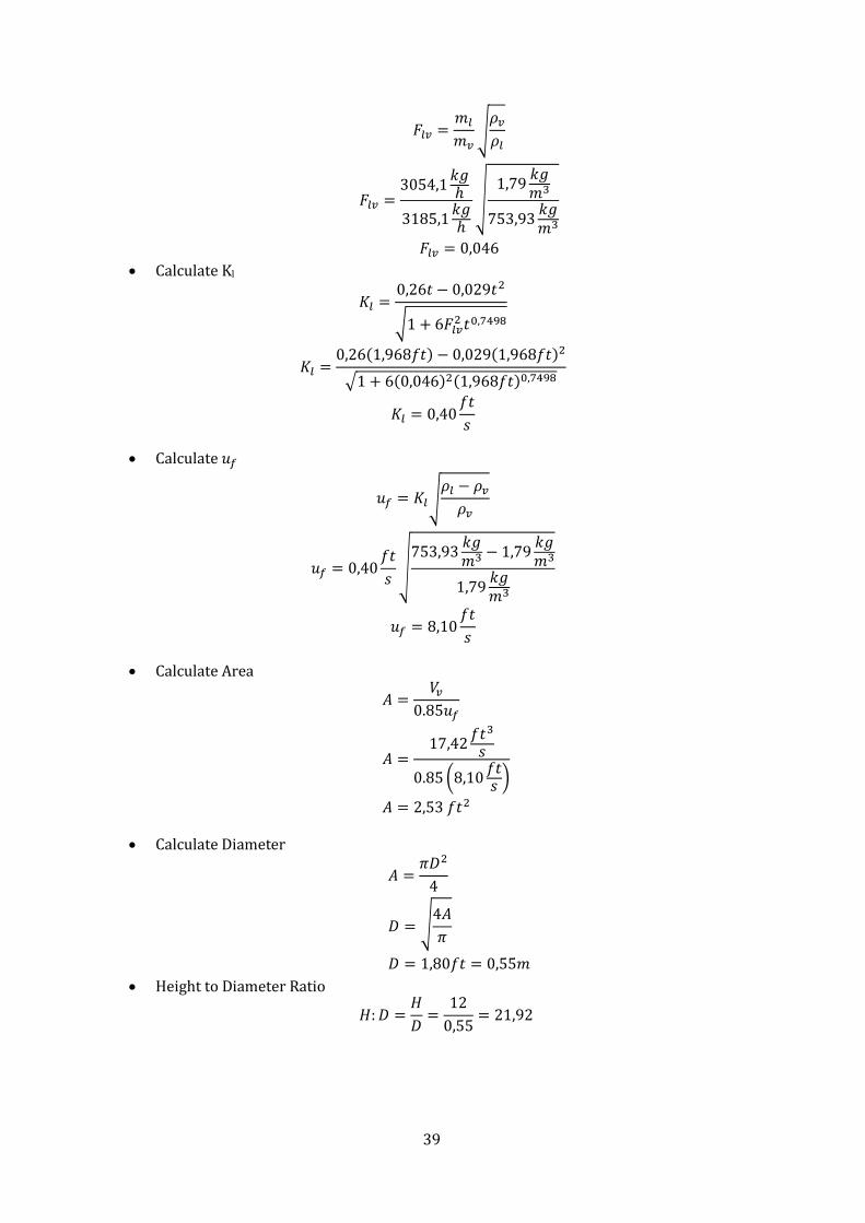
39

𝐹𝑙𝑣 =𝑚𝑙

𝑚𝑣�𝜌𝑣𝜌𝑙

𝐹𝑙𝑣 =3054,1𝑘𝑘ℎ

3185,1𝑘𝑘ℎ

�1,79 𝑘𝑘𝑚3

753,93 𝑘𝑘𝑚3

𝐹𝑙𝑣 = 0,046 • Calculate Kl

𝐾𝑙 =0,26𝑡 − 0,029𝑡2

�1 + 6𝐹𝑙𝑣2 𝑡0,7498

𝐾𝑙 =0,26(1,968𝑓𝑡) − 0,029(1,968𝑓𝑡)2

�1 + 6(0,046)2(1,968𝑓𝑡)0,7498

𝐾𝑙 = 0,40𝑓𝑡𝑠

• Calculate 𝑢𝑓

𝑢𝑓 = 𝐾𝑙�𝜌𝑙 − 𝜌𝑣𝜌𝑣

𝑢𝑓 = 0,40𝑓𝑡𝑠�

753,93 𝑘𝑘𝑚3 − 1,79 𝑘𝑘𝑚3

1,79 𝑘𝑘𝑚3

𝑢𝑓 = 8,10𝑓𝑡𝑠

• Calculate Area

𝐴 =𝑉𝑣

0.85𝑢𝑓

𝐴 =17,42𝑓𝑡

3

𝑠0.85 �8,10𝑓𝑡𝑠 �

𝐴 = 2,53 𝑓𝑡2

• Calculate Diameter

𝐴 =𝜋𝐷2

4

𝐷 = �4𝐴𝜋

𝐷 = 1,80𝑓𝑡 = 0,55𝑚 • Height to Diameter Ratio

𝐻:𝐷 =𝐻𝐷

=12

0,55= 21,92

40

Extraction Column Diameter

𝐷𝑐 = �4 ∗ (𝑄𝑐 + 𝑄𝑑)𝜋 ∗ 𝑘 ∗ 𝐵𝑚𝑚𝑚

(4)

Equation 4 shows how the diameter of the column is calculated. The volumetric flows of water

and oil are predetermined using Aspen, and k represents the flooding coefficient, which is

assumed to be 0.8. Thus, only the flooding capacity, Bmax, must be determined. The flooding

capacity is the sum of the flooding velocities of oil and water. Equation 5 is used to calculate

these.

𝑣𝑓𝑙𝑓𝑓𝑑 = 𝐶𝐹𝑚𝐹𝐹 �𝜎

20�0.20

�𝜌𝐿 − 𝜌𝑉𝜌𝑉

(5)

To use equation 5, the density and surface tension of oil and water must be known, which is

shown by Table 23. Oil is assumed to be n-hexadecane.

Table 23: Physical parameters of the two phases in the extraction column (Sigma Aldrich, 2014)

Surface Tension (dyn/cm) Density (kg/m3)

n-hexadecane 27.47 770 Water 72.8 999.97

Cfair constant is determined to be 0.15 m/s, thus:

𝑣ℎ𝑒𝑚𝑚𝑒𝑒 = 0.15𝑚𝑠�

27.4720

�0.20

∗ �999.97− 770

770= 0.087

ms

Similarly, vwater is equal to 0.106 m/s, making Bmax equal to 0.193. Using equation 5:

𝐷𝐶 = ��4 ∗ �1.86𝑚

3

𝑠 + 0.006𝑚3

𝑠 ��

𝜋 ∗ 0.8 ∗ 0.193𝑚𝑠= 3.92 𝑚 ≅ 4 𝑚

Surface Area for Heat Exchange 𝑄 = 𝑈𝐴Δ𝑇 (6)

By rearranging Equation 6 for A, surface area, the following equation is formed:

41

𝐴 =𝑄

(𝑈∆𝑇)

For the Block 13 heat exchanger, the following data can be plugged in

𝐴 =1076000 W

1000 𝑊𝑚2𝐾 ∗ 108 𝐾

= 9.96 𝑚2

A similar method can be used for the “block 6” heat exchanger.

NPV Calculation

𝑁𝑃𝑉 = −𝐺 + 𝐴𝐹 ∗�(1 + 𝐼)−𝑁𝑁

𝐹=1

Data Tables

Plant Costs (Ulrich Estimations)

Table 24: Ulrich cost estimation for Distillation Column 2 (EconExpert, 2000)

DISTILLATION COLUMN 2 Cost Summary

The cost index is 579.7

Process Vessels (including towers) : Vertically oriented : With sieve-trays Total purchased cost = $ 28152

Material factor = 1.00

Trays 15 Material factor for tower packing = 2.20

Height 9

The bare module cost of tower packing is = $ 19875 Diameter 0.76 The bare module cost is = $ 140525

Pressure 1

Total Bare Module Cost = $ 140525

Contingency and Fee = $ 25294

Total Module Cost = $ 165819

Auxiliary Facilities = $ 49746

Grass Roots Capital = $ 215565

42

Table 25: Ulrich cost estimation for Inline Mixer 1 and 2 (EconExpert, 2000)

INLINE MIXER 1 INLINE MIXER 2 Cost Summary

Cost Summary

The cost index is 579.7 The cost index is 579.7

Mixers : Agitators and Inline Mixers : Inline Mixers : Agitators and Inline Mixers : Inline Total purchased cost = $ 9402 Total purchased cost = $ 26240 The bare module cost is = $ 32907 The bare module cost is = $ 91840

Total Bare Module Cost = $ 32907 Total Bare Module Cost = $ 91840 Contingency and Fee = $ 5923 Contingency and Fee = $ 16531 Total Module Cost = $ 38831 Total Module Cost = $ 108371 Auxiliary Facilities = $ 11649 Auxiliary Facilities = $ 32511 Grass Roots Capital = $ 50480 Grass Roots Capital = $ 140883

POWER 1.5KW

POWER 22.37 KW

Table 26: Ulrich cost estimation for the centrifugal pump (EconExpert, 2000)

Pump 1 Cost Summary

The cost index is 579.7

Pumps : Centrifugal

Total purchased cost = $ 5712

Material factor = 1.90

Pressure factor = 1.00

The bare module cost (incl. electric motor drive) is = $ 27567

Total Bare Module Cost = $ 27567

Contingency and Fee = $ 4962

Total Module Cost = $ 32529

Auxiliary Facilities = $ 9759

Grass Roots Capital = $ 42288

P=2 BARS 1.151KW

43

Table 27: Ulrich cost estimation for Heat Exchanger B13 (EconExpert, 2000)

HEAT EXCHANGER B13 Cost Summary

http://www.thermopedia.com/content/841/ The cost index is 579.7

Heat Exchangers : Shell and Tube : Kettle reboiler Total purchased cost = $ 11040

Material factor = 2.80

Pressure factor = 1.00

The bare module cost is = $ 60969

Total Bare Module Cost = $ 60969

Contingency and Fee = $ 10974

Total Module Cost = $ 71943

Auxiliary Facilities = $ 21583

Grass Roots Capital = $ 93526

p=1bar SA=9.96 U=1000 B13

Table 28: Ulrich cost estimation for Heat Exchanger B6 (EconExpert, 2000)

HEAT EXCHANGER B6 Cost Summary

The cost index is 579.7

Heat Exchangers : Shell and Tube : Kettle reboiler Total purchased cost = $ 11191

Material factor = 2.80

Pressure factor = 1.00

The bare module cost is = $ 61803

Total Bare Module Cost = $ 61803

Contingency and Fee = $ 11124

Total Module Cost = $ 72927

Auxiliary Facilities = $ 21878

Grass Roots Capital = $ 94805

P=1BAR SA=10.34

44

Table 29: Ulrich cost estimation for the Steam Stripper (EconExpert, 2000)

STEAM STRIPPER Cost Summary

The cost index is 579.9

Process Vessels (including towers) : Vertically oriented : With sieve-trays

Total purchased cost = $ 163786 Material factor = 1.00

Material factor for tower packing = 2.20 The bare module cost of tower packing is = $ 316566

The bare module cost is = $ 1018509

Total Bare Module Cost = $ 1018509 Contingency and Fee = $ 183332

Total Module Cost = $ 1201840 Auxiliary Facilities = $ 360552 Grass Roots Capital = $ 1562392 D=2.78 H=26

Table 30: Ulrich cost estimation for the Extraction Column (EconExpert, 2000)

Extraction column 1 bar hieght 30 m

packing material - random polymeric

vessel material - carbon steel

Cost Summary

The cost index is 579.7

Process Vessels (including towers) : Vertically oriented : With tower packings Total purchased cost = $ 239709

Material factor = 1.00

Material factor for tower packing = 1.20

The bare module cost of tower packing is = $ 2250265

The bare module cost is = $ 3277594

Total Bare Module Cost = $ 3277594

Contingency and Fee = $ 589967

Total Module Cost = $ 3867560

Auxiliary Facilities = $ 1160268

Grass Roots Capital = $ 5027829

Stream Conditions

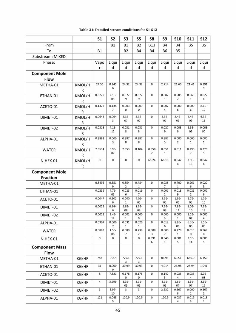
45

Table 31: Detailed stream conditions for S1-S12

S1 S2 S3 S5 S8 S9 S10 S11 S12 From B1 B1 B2 B13 B4 B4 B5 B5

To B1 B2 B4 B4 B6 B5 Substream: MIXED

Phase: Vapor

Liquid

Liquid

Liquid

Liquid

Liquid

Liquid

Liquid

Liquid

Component Mole Flow

METHA-01 KMOL/HR

24.56 0.2456

24.32 24.32 0 2.714 21.60 21.41 0.1919

ETHAN-01 KMOL/HR

0.6729 2.1E-05

0.6729

0.6729

0 0.0871

0.5857

0.5631

0.0226

ACETO-01 KMOL/HR

0.1377 0.1347

0.0030

0.0030

0 0.0024

0.0006

0.0006

8.6E-10

DIMET-01 KMOL/HR

0.0643 0.0643

5.3E-07

5.3E-07

0 5.3E-07

2.4E-09

2.4E-09

6.3E-18

DIMET-02 KMOL/HR

0.0318 4.1E-12

0.0318

0.0318

0 0.0279

0.0039

2.5E-06

0.00390

ALPHA-01 KMOL/HR

0.8882 0.0003

0.8878

0.8878

0 0.8875

0.0002

0.0001

0.0001

WATER KMOL/HR

2.5534 6.9E-07

2.553 8.104 0.5582

0.0511

8.611 0.2907

8.3205

N-HEX-01 KMOL/HR

0 0 0 0 66.24 66.19 0.0474

7.0E-13

0.0474

Component Mole Fraction

METHA-01 0.8495 0.5519

0.8542

0.4841

0 0.0387

0.7001

0.9616

0.0223

ETHAN-01 0.0232 4.7E-05

0.0236

0.0197

0 0.0012

0.0189

0.0252

0.0026

ACETO-01 0.0047 0.3026

0.0001

9.0E-05

0 3.5E-05

1.9E-05

2.7E-05

1.0E-10

DIMET-01 0.0022 0.1446

1.8E-08

1.5E-08

0 7.5E-09

7.8E-11

1.0E-10

7.3E-19

DIMET-02 0.0011 9.4E-12

0.0011

0.0009

0 0.0003

0.0001

1.1E-07

0.0004

ALPHA-01 0.0307 0.0007

0.0311

0.0261

0 0.0126

8.9E-06

6.3E-06

1.5E-05

WATER 0.0883 1.5E-06

0.0897

0.2382

0.0083

0.0007

0.2791

0.0130

0.9690

N-HEX-01 0 0 0 0 0.9916

0.9461

0.0015

3.1E-14

0.0055

Component Mass Flow

METHA-01 KG/HR 787 7.87 779.13

779.13

0 86.95 692.1 686.0 6.150

ETHAN-01 KG/HR 31 0.0009

30.99 30.99 0 4.014 26.98 25.94 1.041

ACETO-01 KG/HR 8 7.821 0.1780

0.1780

0 0.1425

0.0354

0.0354

5.0E-08

DIMET-01 KG/HR 4 3.999 3.3E-05

3.3E-05

0 3.3E-05

1.5E-07

1.5E-07

3.9E-16

DIMET-02 KG/HR 3 3.9E-10

3 3 0 2.632 0.3678

0.0002

0.3675

ALPHA-01 KG/HR 121 0.0455

120.9 120.9 0 120.9 0.0374

0.0193

0.0181

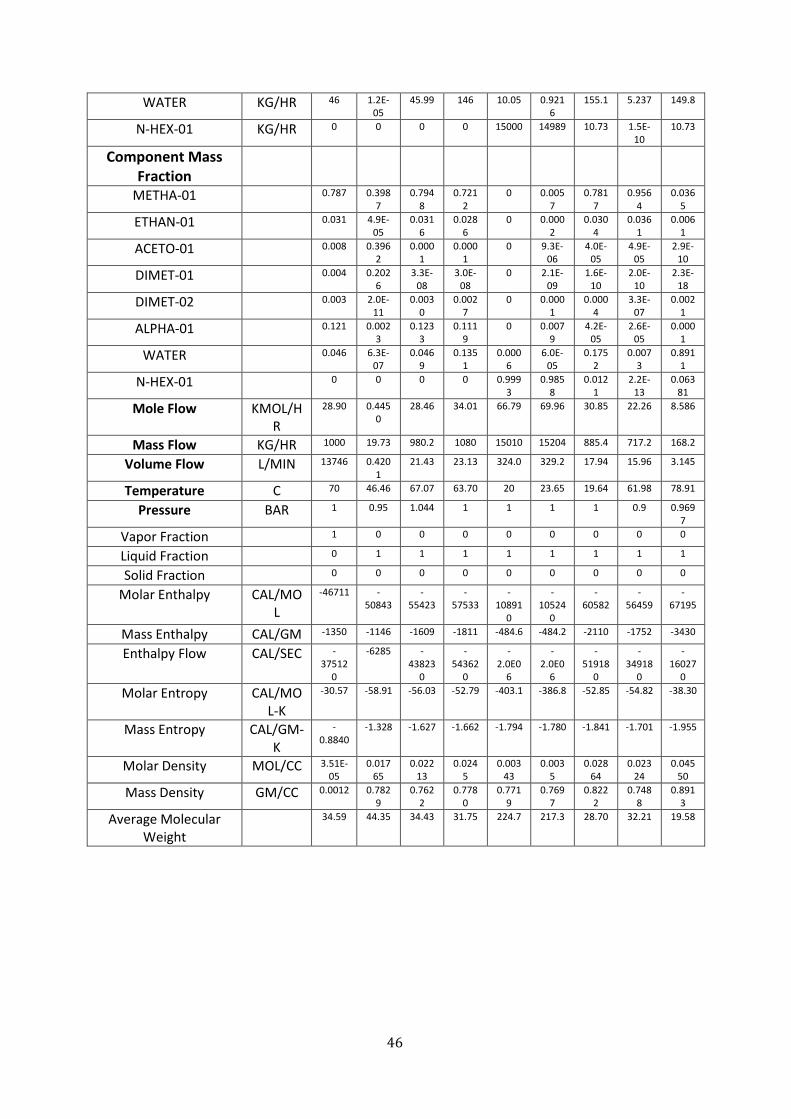
46

WATER KG/HR 46 1.2E-05

45.99 146 10.05 0.9216

155.1 5.237 149.8

N-HEX-01 KG/HR 0 0 0 0 15000 14989 10.73 1.5E-10

10.73

Component Mass Fraction

METHA-01 0.787 0.3987

0.7948

0.7212

0 0.0057

0.7817

0.9564

0.0365

ETHAN-01 0.031 4.9E-05

0.0316

0.0286

0 0.0002

0.0304

0.0361

0.0061

ACETO-01 0.008 0.3962

0.0001

0.0001

0 9.3E-06

4.0E-05

4.9E-05

2.9E-10

DIMET-01 0.004 0.2026

3.3E-08

3.0E-08

0 2.1E-09

1.6E-10

2.0E-10

2.3E-18

DIMET-02 0.003 2.0E-11

0.0030

0.0027

0 0.0001

0.0004

3.3E-07

0.0021

ALPHA-01 0.121 0.0023

0.1233

0.1119

0 0.0079

4.2E-05

2.6E-05

0.0001

WATER 0.046 6.3E-07

0.0469

0.1351

0.0006

6.0E-05

0.1752

0.0073

0.8911

N-HEX-01 0 0 0 0 0.9993

0.9858

0.0121

2.2E-13

0.06381

Mole Flow KMOL/HR

28.90 0.4450

28.46 34.01 66.79 69.96 30.85 22.26 8.586

Mass Flow KG/HR 1000 19.73 980.2 1080 15010 15204 885.4 717.2 168.2

Volume Flow L/MIN 13746 0.4201

21.43 23.13 324.0 329.2 17.94 15.96 3.145

Temperature C 70 46.46 67.07 63.70 20 23.65 19.64 61.98 78.91

Pressure BAR 1 0.95 1.044 1 1 1 1 0.9 0.9697

Vapor Fraction 1 0 0 0 0 0 0 0 0

Liquid Fraction 0 1 1 1 1 1 1 1 1

Solid Fraction 0 0 0 0 0 0 0 0 0

Molar Enthalpy CAL/MOL

-46711 -50843

-55423

-57533

-10891

0

-10524

0

-60582

-56459

-67195

Mass Enthalpy CAL/GM -1350 -1146 -1609 -1811 -484.6 -484.2 -2110 -1752 -3430

Enthalpy Flow CAL/SEC -37512

0

-6285 -43823

0

-54362

0

-2.0E0

6

-2.0E0

6

-51918

0

-34918

0

-16027

0

Molar Entropy CAL/MOL-K

-30.57 -58.91 -56.03 -52.79 -403.1 -386.8 -52.85 -54.82 -38.30

Mass Entropy CAL/GM-K

-0.8840

-1.328 -1.627 -1.662 -1.794 -1.780 -1.841 -1.701 -1.955

Molar Density MOL/CC 3.51E-05

0.01765

0.02213

0.0245

0.00343

0.0035

0.02864

0.02324

0.04550

Mass Density GM/CC 0.0012 0.7829

0.7622

0.7780

0.7719

0.7697

0.8222

0.7488

0.8913

Average Molecular Weight

34.59 44.35 34.43 31.75 224.7 217.3 28.70 32.21 19.58

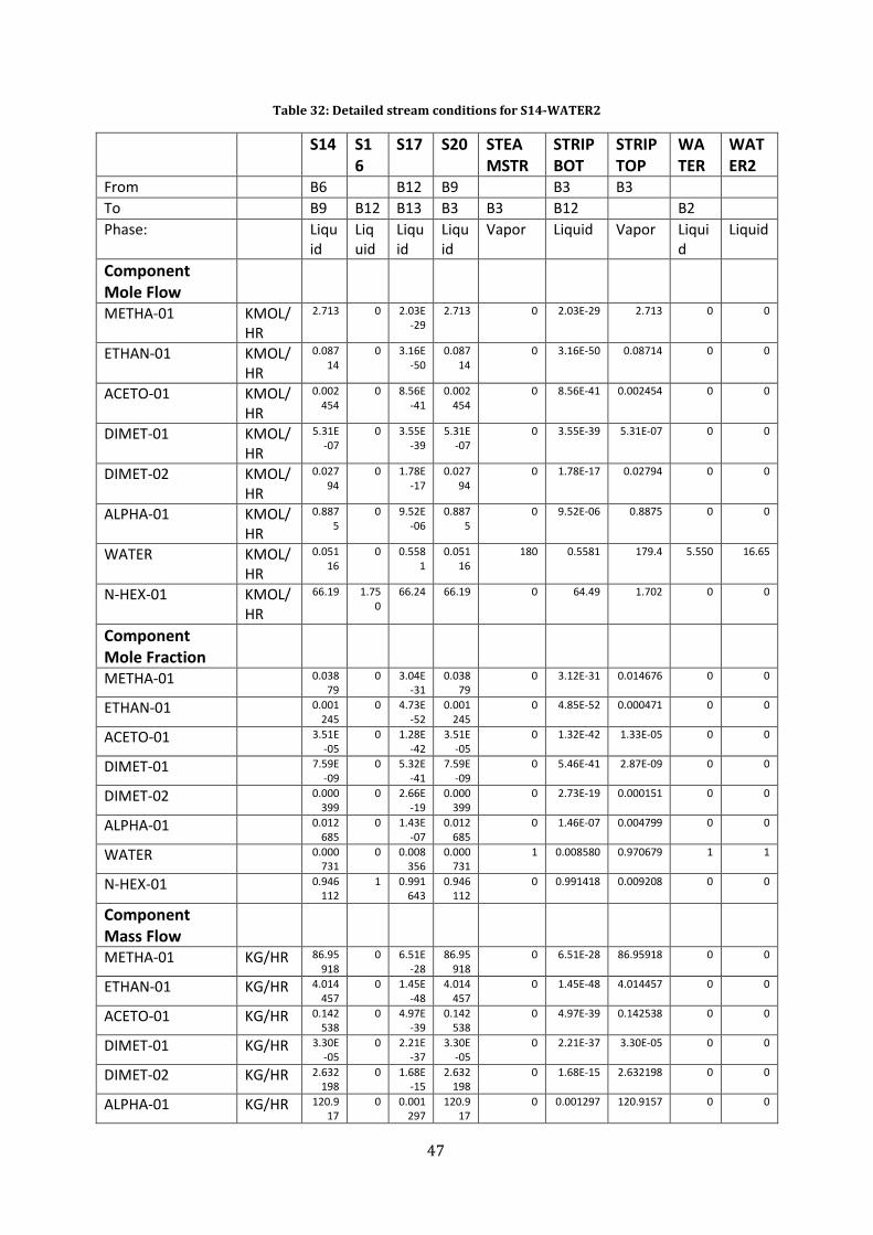
47

Table 32: Detailed stream conditions for S14-WATER2

S14 S16

S17 S20 STEAMSTR

STRIPBOT

STRIPTOP

WATER

WATER2

From B6 B12 B9 B3 B3 To B9 B12 B13 B3 B3 B12 B2 Phase: Liqu

id Liquid

Liquid

Liquid

Vapor Liquid Vapor Liquid

Liquid

Component Mole Flow

METHA-01 KMOL/HR

2.713 0 2.03E-29

2.713 0 2.03E-29 2.713 0 0

ETHAN-01 KMOL/HR

0.08714

0 3.16E-50

0.08714

0 3.16E-50 0.08714 0 0

ACETO-01 KMOL/HR

0.002454

0 8.56E-41

0.002454

0 8.56E-41 0.002454 0 0

DIMET-01 KMOL/HR

5.31E-07

0 3.55E-39

5.31E-07

0 3.55E-39 5.31E-07 0 0

DIMET-02 KMOL/HR

0.02794

0 1.78E-17

0.02794

0 1.78E-17 0.02794 0 0

ALPHA-01 KMOL/HR

0.8875

0 9.52E-06

0.8875

0 9.52E-06 0.8875 0 0

WATER KMOL/HR

0.05116

0 0.5581

0.05116

180 0.5581 179.4 5.550 16.65

N-HEX-01 KMOL/HR

66.19 1.750

66.24 66.19 0 64.49 1.702 0 0

Component Mole Fraction

METHA-01 0.03879

0 3.04E-31

0.03879

0 3.12E-31 0.014676 0 0

ETHAN-01 0.001245

0 4.73E-52

0.001245

0 4.85E-52 0.000471 0 0

ACETO-01 3.51E-05

0 1.28E-42

3.51E-05

0 1.32E-42 1.33E-05 0 0

DIMET-01 7.59E-09

0 5.32E-41

7.59E-09

0 5.46E-41 2.87E-09 0 0

DIMET-02 0.000399

0 2.66E-19

0.000399

0 2.73E-19 0.000151 0 0

ALPHA-01 0.012685

0 1.43E-07

0.012685

0 1.46E-07 0.004799 0 0

WATER 0.000731

0 0.008356

0.000731

1 0.008580 0.970679 1 1

N-HEX-01 0.946112

1 0.991643

0.946112

0 0.991418 0.009208 0 0

Component Mass Flow

METHA-01 KG/HR 86.95918

0 6.51E-28

86.95918

0 6.51E-28 86.95918 0 0

ETHAN-01 KG/HR 4.014457

0 1.45E-48

4.014457

0 1.45E-48 4.014457 0 0

ACETO-01 KG/HR 0.142538

0 4.97E-39

0.142538

0 4.97E-39 0.142538 0 0

DIMET-01 KG/HR 3.30E-05

0 2.21E-37

3.30E-05

0 2.21E-37 3.30E-05 0 0

DIMET-02 KG/HR 2.632198

0 1.68E-15

2.632198

0 1.68E-15 2.632198 0 0

ALPHA-01 KG/HR 120.917

0 0.001297

120.917

0 0.001297 120.9157 0 0

48

WATER KG/HR 0.921692

0 10.05579

0.921692

3242.75 10.05579 3233.616 100 300

N-HEX-01 KG/HR 14989.27

396.309

14999.97

14989.27

0 14603.66 385.6022 0 0

Component Mass Fraction

METHA-01 0.00571

0 4.34E-32

0.00571

0 4.45E-32 0.022681 0 0

ETHAN-01 0.00026

0 9.69E-53

0.00026

0 9.95E-53 0.001047 0 0

ACETO-01 9.3E-06

0 3.31E-43

9.3E-06

0 3.40E-43 3.72E-05 0 0

DIMET-01 2.1E-09

0 1.47E-41

2.1E-09

0 1.51E-41 8.61E-09 0 0

DIMET-02 0.0001

0 1.12E-19

0.00017

0 1.15E-19 0.000686 0 0

ALPHA-01 0.00795

0 8.64E-08

0.00795

0 8.88E-08 0.031538 0 0

WATER 6.0E-05

0 0.00066

6.0E-05

1 0.000688 0.843431 1 1

N-HEX-01 0.98582

1 0.99933

0.98582

0 0.999311 0.100577 0 0

Mole Flow KMOL/HR

69.9637

1.75012

66.7990

69.9637

180 65.04891 184.9148 5.5508 16.6525

Mass Flow KG/HR 15204.8

396.309

15010.0

15204.8

3242.75 14613.72 3833.883 100 300

Volume Flow L/MIN 366.978

8.55404

357.800

367.018

78566.6 349.3187 111469 1.6687 5.00617

Temperature C 140 20 128.356

140.102

104.8316 131.0616 140.116 20 20

Pressure BAR 1 1 1 2 1.2 1.044654 0.95 1 1

Vapor Fraction 0 0 0 0 1 0 1 0 0

Liquid Fraction 1 1 1 1 0 1 0 1 1

Solid Fraction 0 0 0 0 0 0 0 0 0

Molar Enthalpy CAL/MOL

-9048

4

-1.0E

06

-9505

0

-9047

0

-57112.8 -94666.39

-56523.36

-68350 -68350

Mass Enthalpy CAL/GM

-416.3

5

-482.

74

-423.0

0

-416.2

9

-3170.242 -421.3811

-2726.219

-3794.0

-3794.03

Enthalpy Flow CAL/SEC

-1.7E0

6

-5314

3

-1.7E0

6

-1.7E0

6

-2855600 -1710500 -2903300 -1.0E05

-316170

Molar Entropy CAL/MOL-K

-345.1

6

-406.

39

-363.0

6

-345.1

2

-9.032567 -362.0526

-11.40727

-39.26 -39.26

Mass Entropy CAL/GM-K

-1.588

2

-1.79

46

-1.615

7

-1.588

0

-0.5013836

-1.611576

-0.55019 -2.1794

-2.1794

Molar Density MOL/CC

0.0031

0.0034

0.0031

0.0031

3.82E-05 0.0031036

2.76E-05 0.0554 0.05544

Mass Density GM/CC 0.690 0.772

0.699 0.6904

0.00068789

0.6972487

0.0005732

0.99876

0.998767

Average Molecular Weight

217.32

226.4

224.70

217.32

18.01528 224.6574 20.73324 18.0152

18.01528

49

Unit Operating Conditions B1 - Distillation Column 1

Top Stage Temperature 46.4611115 C Heat duty -136807.949 cal/sec Distillate rate 0.445020567 kmol/hr Reflux rate 61.9355354 kmol/hr Reflux ratio 139.174546

Bottom Stage Temperature 67.071943 C Heat duty 67410.9479 cal/sec Bottoms rate 28.4647816 kmol/hr Boilup rate 28.4647816 kmol/hr Boilup ratio 1

B2 - Inline Mixer 1 Outlet Temp 63.701 C

Pressure 1 bar Vapour Fraction 0

1st Liquid/Total Liquid 1

B3 - Steam Stripper Top Stage

Temperature 140.115998 C Heat duty 0 cal/sec Distillate rate 184.9148 kmol/hr Reflux rate 67.2220849 kmol/hr Reflux ratio 0.363530042

Bottom Stage Temperature 131.061646 C Heat duty 0 cal/sec Bottoms rate 65.0489101 kmol/hr Boilup rate 180.956318 kmol/hr Boilup ratio 2.78185012

B4 - Extraction Column Top stage Temp 23.658 C

Top Stage 1st Liquid Flow 32.663 kmol/h Top Stage 2nd Liquid Flow 69.964 kmol/h

Bottom Stage Temp 19.646 C Bottom Stage 1st Liquid Flow 30.851 kmol/h Bottom Stage 2nd Liquid Flow 68.611 kmol/h

50

B5 - Distillation Column 2 Top Stage

Temperature 61.9873133 C Heat duty -105666.457 cal/sec Distillate rate 22.264533 kmol/hr Reflux rate 22.264533 kmol/hr Reflux ratio 1

Bottom Stage Temperature 78.9107205 C Heat duty 115398.741 cal/sec Bottoms rate 8.58653398 kmol/hr Boilup rate 34.021406 kmol/hr Boilup ratio 3.96218149

B6 - Heat Exchanger 1 Outlet Temp 140 C

Pressure 1 bar Vapour Fraction 0

Heat Duty 286840.795 cal/sec Net Duty 286840.795 cal/sec

1st Liquid/Total Liquid 1

B9 - Pump Fluid Power 0.6116 kW Brake Power 1.1509 kW

Electricity 1.1509 kW Volumetric Flow Rate 366.979 L/min

Pressure Change 1 bar NPSH Available 5.0137 m-kgf/kg

Head Developed 14.767 m-kgf/kg Pump Efficiency 0.5314

Net Work Required 1.1509 kW

B12 - Inline Mixer 2 Outlet Temp 128.357 C

Pressure 1 bar Vapour Fraction 0

1st Liquid/Total Liquid 1

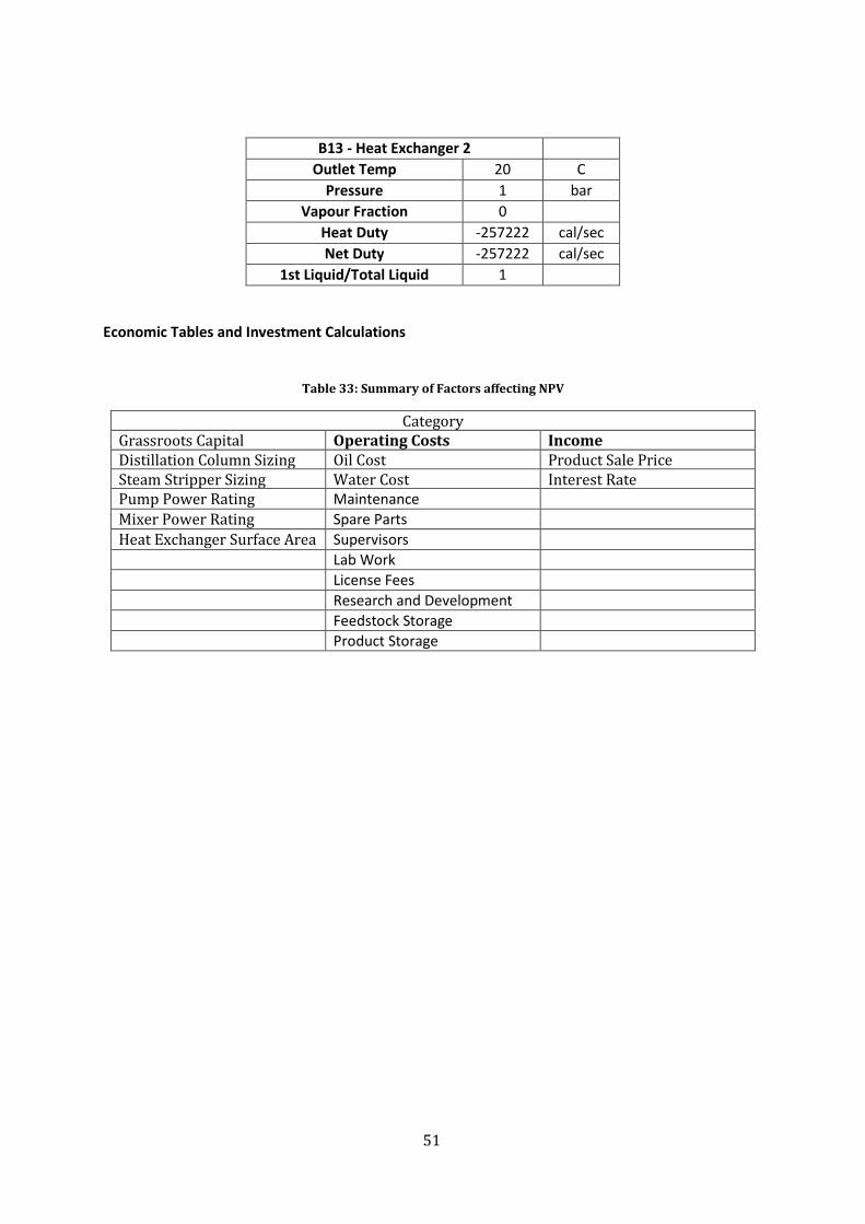
51

B13 - Heat Exchanger 2 Outlet Temp 20 C

Pressure 1 bar Vapour Fraction 0

Heat Duty -257222 cal/sec Net Duty -257222 cal/sec

1st Liquid/Total Liquid 1

Economic Tables and Investment Calculations

Table 33: Summary of Factors affecting NPV

Category Grassroots Capital Operating Costs Income Distillation Column Sizing Oil Cost Product Sale Price Steam Stripper Sizing Water Cost Interest Rate Pump Power Rating Maintenance Mixer Power Rating Spare Parts Heat Exchanger Surface Area Supervisors Lab Work License Fees Research and Development Feedstock Storage Product Storage

52

Table 34: NPV and Pay off time calculation summary

Year NPV (SEK) 1 -52,903,765.41 2 -43,303,668.31 3 -34,654,932.18 4 -26,863,278.01 5 -19,843,769.75 6 -13,519,888.43 7 -7,822,698.06 8 -2,690,094.12 9 1,933,873.40 10 6,099,609.90 11 9,852,525.66 12 13,233,530.86 13 16,279,481.48 14 19,023,581.14 15 21,495,743.00 16 23,722,915.85 17 25,729,377.87 18 27,537,001.31 19 29,165,490.90 20 30,632,598.64