
frequentist: Asymptotic expansions
23
arXiv:math.ST/0611671 v1 22 Nov 2006 IMS Lecture Notes–Monograph Series Recent Developments in Nonparametric Inference and Probability Vol. 50 (2006) 190–212 c Institute of Mathematical Statistics, 2006 DOI: 10.1214/074921706000000699 On the false discovery rates of a frequentist: Asymptotic expansions Anirban DasGupta 1 Tonglin Zhang 2 Purdue University Abstract: Consider a testing problem for the null hypothesis H 0 : θ ∈ Θ 0 . The standard frequentist practice is to reject the null hypothesis when the p- value is smaller than a threshold value α, usually 0.05. We ask the question how many of the null hypotheses a frequentist rejects are actually true. Precisely, we look at the Bayesian false discovery rate δn = Pg (θ ∈ Θ 0 |p − value < α) under a proper prior density g(θ). This depends on the prior g, the sample size n, the threshold value α as well as the choice of the test statistic. We show that the Benjamini–Hochberg FDR in fact converges to δn almost surely under g for any fixed n. For one-sided null hypotheses, we derive a third order asymptotic expansion for δn in the continuous exponential family when the test statistic is the MLE and in the location family when the test statistic is the sample median. We also briefly mention the expansion in the uniform family when the test statistic is the MLE. The expansions are derived by putting together Edgeworth expansions for the CDF, Cornish–Fisher expansions for the quantile function and various Taylor expansions. Numerical results show that the expansions are very accurate even for a small value of n (e.g., n = 10). We make many useful conclusions from these expansions, and specifically that the frequentist is not prone to false discoveries except when the prior g is too spiky. The results are illustrated by many examples. 1. Introduction In a strikingly interesting short note, Sori´ c [19] raised the question of establishing upper bounds on the proportion of fictitious statistical discoveries in a battery of independent experiments. Thus, if m null hypotheses are tested independently, of which m 0 happen to be true, but V among these m 0 are rejected at a significance level α, and another S among the false ones are also rejected, Sori´ c essentially suggested E(V )/(V + S) as a measure of the false discovery rate in the chain of m independent experiments. Benjamini and Hochberg [3] then looked at the question in much greater detail and gave a careful discussion for what a correct formulation for the false discovery rate of a group of frequentists should be, and provided a concrete procedure that actually physically controls the groupwise false discovery rate. The problem is simultaneously theoretically attractive, socially relevant, and practically important. The practical importance comes from its obvious relation to statistical discoveries made in clinical trials, and in modern microarray experiments. The continued importance of the problem is reflected in two recent articles, Efron [7], and Storey [21], who provide serious Bayesian connections and advancements 1 Department of Statistics, Purdue University, 150 North University Street, West Lafayette, IN 47907-2067, e-mail: [email protected] 2 Department of Statistics, Purdue University, 150 North University Street, West Lafayette, IN 47907-2067, e-mail: [email protected] AMS 2000 subject classifications: primary 62F05; secondary 62F03, 62F15. Keywords and phrases: Cornish–Fisher expansions, Edgeworth expansions, exponential fami- lies, false discovery rate, location families, MLE, p-value. 190
Transcript of frequentist: Asymptotic expansions
arX
iv:m
ath.
ST/0
6116
71 v
1 2
2 N
ov 2
006
IMS Lecture Notes–Monograph Series
Recent Developments in Nonparametric Inference and Probability
Vol. 50 (2006) 190–212c© Institute of Mathematical Statistics, 2006DOI: 10.1214/074921706000000699
On the false discovery rates of a
frequentist: Asymptotic expansions
Anirban DasGupta1 Tonglin Zhang2
Purdue University
Abstract: Consider a testing problem for the null hypothesis H0 : θ ∈ Θ0.The standard frequentist practice is to reject the null hypothesis when the p-value is smaller than a threshold value α, usually 0.05. We ask the question howmany of the null hypotheses a frequentist rejects are actually true. Precisely,we look at the Bayesian false discovery rate δn = Pg(θ ∈ Θ0|p − value < α)under a proper prior density g(θ). This depends on the prior g, the samplesize n, the threshold value α as well as the choice of the test statistic. Weshow that the Benjamini–Hochberg FDR in fact converges to δn almost surelyunder g for any fixed n. For one-sided null hypotheses, we derive a third orderasymptotic expansion for δn in the continuous exponential family when the teststatistic is the MLE and in the location family when the test statistic is thesample median. We also briefly mention the expansion in the uniform familywhen the test statistic is the MLE. The expansions are derived by puttingtogether Edgeworth expansions for the CDF, Cornish–Fisher expansions forthe quantile function and various Taylor expansions. Numerical results showthat the expansions are very accurate even for a small value of n (e.g., n = 10).We make many useful conclusions from these expansions, and specifically thatthe frequentist is not prone to false discoveries except when the prior g is toospiky. The results are illustrated by many examples.
1. Introduction
In a strikingly interesting short note, Soric [19] raised the question of establishingupper bounds on the proportion of fictitious statistical discoveries in a battery ofindependent experiments. Thus, if m null hypotheses are tested independently, ofwhich m0 happen to be true, but V among these m0 are rejected at a significancelevel α, and another S among the false ones are also rejected, Soric essentiallysuggested E(V )/(V + S) as a measure of the false discovery rate in the chain of mindependent experiments. Benjamini and Hochberg [3] then looked at the questionin much greater detail and gave a careful discussion for what a correct formulationfor the false discovery rate of a group of frequentists should be, and provided aconcrete procedure that actually physically controls the groupwise false discoveryrate. The problem is simultaneously theoretically attractive, socially relevant, andpractically important. The practical importance comes from its obvious relation tostatistical discoveries made in clinical trials, and in modern microarray experiments.The continued importance of the problem is reflected in two recent articles, Efron[7], and Storey [21], who provide serious Bayesian connections and advancements
1Department of Statistics, Purdue University, 150 North University Street, West Lafayette, IN47907-2067, e-mail: [email protected]
2Department of Statistics, Purdue University, 150 North University Street, West Lafayette, IN47907-2067, e-mail: [email protected]
AMS 2000 subject classifications: primary 62F05; secondary 62F03, 62F15.Keywords and phrases: Cornish–Fisher expansions, Edgeworth expansions, exponential fami-
lies, false discovery rate, location families, MLE, p-value.
190
False discovery rates of a frequentist 191
in the problem. See also Storey [20], Storey, Taylor and Siegmund [22], Storey andTibshirani [23], Genovese and Wasserman [10], and Finner and Roters [9], amongmany others in this currently active area.
Around the same time that Soric raised the issue of fictitious frequentist dis-coveries made by a mechanical adoption of the use of p-values, a different debatewas brewing in the foundation literature. Berger and Sellke [2], in a thought pro-voking article, gave analytical foundations to the thesis in Edwards, Lindman andSavage [6] that the frequentist practice of rejecting a sharp null at a traditional5% level amounts to a rush to judgment against the null hypothesis. By derivinglower bounds or exact values for the minimum value of the posterior probability of asharp null hypothesis over a variety of classes of priors, Berger and Sellke [2] arguedthat p-values traditionally regarded as small understate the plausibility of nulls, atleast in some problems. Casella and Berger [5], gave a collection of theorems thatshow that the discrepancy disappears under broad conditions if the null hypothesisis composite one-sided. Since the articles of Berger and Sellke [2] and Casella andBerger [5], there has been an avalanche of activity in the foundation literature onthe safety of use of p-values in testing problems. See Hall and Sellinger [12], Sel-lke, Bayarri and Berger [18], Marden [14] and Schervish [17] for a contemporaryexposition.
It is conceptually clear that the frequentist FDR literature and the foundationliterature were both talking about a similar issue: is the frequentist practice ofrejecting nulls at traditional p-values an invitation to rampant false discoveries? Thestructural difference was that the FDR literature did not introduce a formal prioron the unknown parameters, while the foundation literature did not go into multipletesting, as is the case in microarray or other emerging interesting applications. Thepurpose of this article is to marry the two schools together, while giving a newrigorous analysis of the interesting question: “how many of the null hypotheses afrequentist rejects are actually trues” and the flip side of that question, namely,“how many of the null hypotheses a frequentist accepts are actually falses”. Thecalculations are completely different from what the previous researchers have done,although we then demonstrate that our formulation directly relates to both thetraditional FDR calculations, and the foundational effort in Berger and Sellke [2],and others. We have thus a dual goal; providing a new approach, and integratingit with the two existing approaches.
In Section 2, we demonstrate the connection in very great generality, withoutpractically any structural assumptions at all. This was comforting. As regards toconcrete results, it seems appropriate to look at the one parameter exponentialfamily, it being the first structured case one would want to investigate. In Section 3,we do so, using the MLE as the test statistic. In Section 4, we look at a generallocation parameter, but using the median as the test statistic. We used the medianfor two reasons. First, for general location parameters, the median is credible as atest statistic, while the mean obviously is not. Second, it is important to investigatethe extent to which the answers depend on the choice of the test statistic; bystudying the median, we get an opportunity to compare the answers for the meanand the median in the special normal case.To be specific, let us consider the onesided testing problem based on an i.i.d. sample X1, . . . , Xn from a distributionfamily with parameter θ in the parameter space Ω which is an interval of R. Withoutloss of generality, we assume Ω = (θ, θ) with −∞ ≤ θ < θ ≤ ∞. We consider thetesting problem
H0 : θ ≤ θ0 vs H1 : θ > θ0,
192 A. DasGupta and T. Zhang
where θ0 ∈ (θ, θ). Suppose the α, 0 < α < 1, level test rejects H0 if Tn ∈ C, whereTn is a test statistic. We study the behavior of the quantities,
δn = P (θ ≤ θ0|Tn ∈ C) = P (H0|p − value < α)
and
ǫn = P (θ > θ0|Tn 6∈ C) = P (H1|p − value ≥ α).
Note that δn and ǫn are inherently Bayesian quantities. By an almost egregiousabuse of nomenclature, we will refer to δn and ǫn as type I and type II errors in thisarticle. Our principal objective is to obtain third order asymptotic expansions forδn and ǫn assuming a Bayesian proper prior for θ. Suppose g(θ) is any sufficientlysmooth proper prior density of θ. In the regular case, the expansion for δn we obtainis like
δn =P (θ ≤ θ0, Tn ∈ C)
P (Tn ∈ C)=
c1√n
+c2
n+
c3
n3/2+ O(n−2),(1)
and the expansion for ǫn is like
ǫn =P (θ > θ0, Tn 6∈ C)
P (Tn 6∈ C)=
d1√n
+d2
n+
d3
n3/2+ O(n−2),(2)
where the coefficients c1, c2, c3, d1, d2, and d3 depend on the problem, the teststatistic Tn, the value of α and the prior density g(θ). In the nonregular case,the expansion differs qualitatively; for both δn and ǫn the successive terms are inpowers of 1/n instead of the powers of 1/
√n. Our ability to derive a third order
expansion results in a surprisingly accurate expansion, sometimes for n as small asn = 4. The asymptotic expansions we derive are not just of theoretical interest; theexpansions let us conclude interesting things, as in Sections 3.2 and 4.5, that wouldbe impossible to conclude from the exact expressions for δn and ǫn.
The expansions of δn and ǫn require the expansions of the numerators and thedenominators of (1) and (2) respectively. In the regular case, the expansion of thenumerator of (1) is like
An = P (θ ≤ θ0, Tn ∈ C) =a1√n
+a2
n+
a3
n3/2+ O(n−2)(3)
and the expansion of the numerator of (2) is like
An = P (θ > θ0, Tn 6∈ C) =a1√n
+a2
n+
a3
n3/2+ O(n−2).(4)
Then, the expansion of the denominator of (1) is
Bn = P (Tn ∈ C) = An + λ − An = λ − b1√n− b2
n− b3
n3/2+ O(n−2),(5)
where λ = P (θ > θ0) =∫ θ
θ0g(θ)dθ and assume 0 < λ < 1, b1 = a1−a1, b2 = a2−a2
and b3 = a3 − a3, and the expansion of the denominator of (2) is
Bn = P (Tn 6∈ C) = 1 − Bn = 1 − λ +b1√n
+b2
n+
b3
n3/2+ O(n−2).(6)
False discovery rates of a frequentist 193
Then, we have
c1 =a1
λ, c2 =
a1b1
λ2+
a2
λ, c3 =
a3
λ+
a1b2 + a2b1
λ2+
a1b21
λ3,
(7)
d1 =a1
1 − λ, d2 =
a2
1 − λ− a1b1
(1 − λ)2, d3 =
a3
1 − λ− a2b1 + a1b2
(1 − λ)2+
a1b21
(1 − λ)3.
We will frequently use the three notations in the expansions: the standard normalPDF φ, the standard normal CDF Φ and the standard normal upper α quantilezα = Φ−1(1 − α).
The principal ingredients of our calculations are Edgeworth expansions, Cornish–Fisher expansions and Taylor expansions. The derivation of the expansions becamevery complex. But in the end, we learn a number of interesting things. We learn thattypically the false discovery rate δn is small, and smaller than the pre-experimentalclaim α for quite small n. We learn that typically ǫn > δn, so that the frequentist isless vulnerable to false discovery than to false acceptance. We learn that only pri-ors very spiky at the boundary between H0 and H1 can cause large false discoveryrates. We also learn that these phenomena do not really change if the test statisticis changed. So while the article is technically complex and the calculations are long,the consequences are rewarding. The analogous expansions are qualitatively differ-ent in the nonregular case. We could not report them here due to shortage of space.We should also add that we leave open the question of establishing these expan-sions for problems with nuisance parameters, multivariate problems, and dependentdata. Results similar to ours are expected in such problems.
2. Connection to Benjamini and Hochberg, Storey and Efron’s work
Suppose there are m groups of iid samples Xi1, . . . , Xin for i = 1, . . . , m. AssumeXi1, . . . , Xin are iid with a common density f(x, θi), where θi are assumed iid witha CDF G(θ) which does not need to have a density in this section. Then, the priorG(θ) connects our Bayesian false discovery rate δn to the usual frequentist falsediscovery rate. In the context of our hypothesis testing problem, the frequentistfalse discovery rate, which has been recently discussed by Benjamini and Hochberg[3], Efron [7] and Storey [21], is defined as
FDR = FDR(θ1, . . . , θm) = Eθ1,...,θm
∑mi=1 ITni∈C,θi≤θ0
(∑m
i=1 ITni∈C) ∨ 1
,(8)
where Tni is the test statistic based on the samples Xi1, . . . , Xin. It will be shownbelow that for any fixed n as m → ∞, the frequentist false discovery rate FDR goesto the Bayesian false discovery rate δn almost surely under the prior distributionG(θ).
We will compare the numerators and the denominators of FDR in (8) and δn
in (1) respectively. Since the comparisons are almost identical, we discuss the com-parison between the numerators only. We denote Eθ(·) and Vθ(·) as the conditionalmean and variance given the true parameter θ, and we denote E(·) and V (·) asthe marginal mean and variance under the prior G(θ). Let Yi = ITni∈C,θi≤θ0
. Thengiven θ1, . . . , θm, Yi (i = 1, , . . . , m) are independent Bernoulli random variableswith mean values µi = µi(θi) = Eθi
(Yi), and marginally µi are iid with expectedvalue An in (3). Let
Dm =1
m
m∑
i=1
ITni∈C,θi≤θ0− An =
1
m
m∑
i=1
(Yi − µi) +1
m
m∑
i=1
(µi − An).
194 A. DasGupta and T. Zhang
Note that we assume that θ1, . . . , θm are iid with a common CDF G(θ). The sec-ond term goes to 0 almost surely by the Strong Law of Large Numbers (SLLN)for identically distributed random variables. Note that for any given θ1, . . . , θm,Y1, . . . , Ym are independent but not iid, with Eθi
(Yi) = µi, Vθi(Yi) = µi(1−µi) and
∑−∞i=1 i−2Vθi
(Yi) ≤∑∞
i=1 i−2 < ∞. The first term also goes to 0 almost surely by aSLLN for independent but not iid random variables [15]. Therefore, Dm goes to 0almost surely. The comparison of denominators is handled similarly. Therefore, foralmost all sequences θ1, θ2, . . . ,
∑mi=1 ITni∈C,θi≤θ0
(∑m
i=1 ITni∈C) ∨ 1→ δn
as m → ∞.
Since∑m
i=1 ITni∈C,θi≤θ0≤ (∑m
i=1 ITni≤C)∨ 1, their ratio is uniformly integrable.And so, FDR as defined in (8) also converges to δn as m → ∞ for almost allsequences θ1, θ2, . . . .
This gives a pleasant, exact connection between our approach and the estab-lished indices formulated by the previous researchers. Of course, for fixed m, thefrequentist FDR does not need to be close to our δn.
3. Continuous one-parameter exponential family
Assume the density of the i.i.d. sample X1, . . . , Xn is in the form of a one-parameterexponential family fθ(x) = b(x)eθx−a(θ) for x ∈ X ⊆ R, where the natural spaceΩ of θ is an interval of R and a(θ) = log
∫
X b(x)eθxdx. Without loss of generality,we can assume Ω is open so that one can write Ω = (θ, θ) for −∞ ≤ θ < θ ≤∞. All derivatives of a(θ) exist at every θ ∈ Ω and can be derived by formallydifferentiating under the integral sign ([4], p. 34). This implies that a′(θ) = Eθ(X1),a′′(θ) = V arθ(X1) for every θ ∈ Ω. Let us denote µ(θ) = a′(θ), σ(θ) =
√
a′′(θ),κi(θ) = a(i)(θ) and ρi(θ) = κi(θ)/σi(θ) for i ≥ 3, where a(i)(θ) represents the i-thderivative of a(θ). Then, µ(θ), σ(θ), κi(θ) and ρi(θ) all exist and are continuous atevery θ ∈ Ω ([4], p. 36), and µ(θ) is non-decreasing in θ since a′′(θ) = σ2(θ) ≥ 0 forall θ.
Let µ0 = µ(θ0), σ0 = σ(θ0), κi0 = κi(θ0) and ρi0 = ρi(θ0) for i ≥ 3 and assumeσ0 > 0 . The usual α (0 < α < 1) level UMP test ([13], p. 80) for the testingproblem H0 : θ ≤ θ0 vs HA : θ ≥ θ0 rejects H0 if X ∈ C where
C = X :√
nX − µ0
σ0> kθ0,n,(9)
and kθ0,n is determined from Pθ0√n(X−µ0)/σ0 > kθ0,n = α; limn→∞ kθ0,n = zα.
Let
βn(θ) = Pθ
(√n
X − µ0
σ0> kθ0,n
)
(10)
Then, using the transformation x = σ0√
n(θ − θ0) − zα under the integral signbelow, we have
(11) An =
∫ θ0
θ
βn(θ)g(θ)dθ =1
σ0√
n
∫ −zα
x
βn(θ0 +x + zα
σ0√
n)g(θ0 +
x + zα
σ0√
n)dx
False discovery rates of a frequentist 195
and
An =1
σ0√
n
∫ x
−zα
[1 − βn(θ0 +x + zα
σ0√
n)]g(θ0 +
x + zα
σ0√
n)dx,(12)
where x = σ0√
n(θ − θ0) − zα and x = σ0√
n(θ − θ0) − zα.Since for an interior parameter θ all moments of the exponential family exist and
are continuous in θ, we can find θ1 and θ2 satisfying θ < θ1 < θ0 and θ0 < θ2 < θsuch that for any θ ∈ [θ1, θ2], σ2(θ), κ3(θ), κ4(θ), κ5(θ), g(θ), g′(θ), g′′(θ) andg(3)(θ) are uniformly bounded in absolute values, and the minimum value of σ2(θ)is a positive number. After we pick θ1 and θ2, we partition each of An and An intotwo parts so that one part is negligible in the expansion. Then, the rest of the workin the expansion is to find the coefficients of the second part.
To describe these partitions, we define θ1n = θ0 + (θ1 − θ0)/n1/3, θ2n = θ0 +(θ2 − θ0)/n1/3, x1n = σ0
√n(θ1n − θ0) − zα and x2n = σ0
√n(θ2n − θ0) − zα. Let
An,θ1n=
1
σ0√
n
∫ −zα
x1n
βn(θ0 +x + zα
σ0√
n)g(θ0 +
x + zα
σ0√
n)dx(13)
Rn,θ1n=
1
σ0√
n
∫ x1n
x
βn(θ0 +x + zα
σ0√
n)g(θ0 +
x + zα
σ0√
n)dx,(14)
An,θ2n=
1
σ0√
n
∫ x2n
−zα
[1 − βn(θ0 +x + zα
σ0√
n)]g(θ0 +
x + zα
σ0√
n)dx,(15)
and
Rn,θ2n=
1
σ0√
n
∫ x
x2n
[1 − βn(θ0 +x + zα
σ0√
n)]g(θ0 +
x + zα
σ0√
n)dx.(16)
Then, An = An,θ1n+Rn,θ1n
and An = An,θ2n+Rn,θ2n
. In the appendix, we show that
for any ℓ > 0, limn→∞ nlRn,θ1n= limn→∞ nlRn,θ2n
= 0. Therefore, it is enough to
compute the coefficients of the expansions for An,θ1nand An,θ2n
. Among the steps
for expansions, the key step is to compute the expansions of βn(θ0+(x+zα)/(σ0√
n))when x ∈ [x1n,−zα] and 1 − βn(θ0 + (x + zα)/(σ0
√n)) when x ∈ [−zα, x2n] under
the integral sign, since the expansion of g(θ0 + (x + zα)/(σ0√
n)) in (13) and (15)is easily obtained as
(17) g(θ0 +x + zα
σ0√
n) = g(θ0) + g′(θ0)
x + zα
σ0√
n+
g′′(θ0)
2
(x + zα)2
σ20n
+ O(n−2).
After a lengthy calculation, we have
An,θ1n=
1
σ0√
n
∫ −zα
x1n
[Φ(x) +φ(x)g1(x)√
n+
φ(x)g2(x)
n]
× [g(θ0) + g′(θ0)x + zα
σ0√
n+
g′′(θ0)
2
(x + zα)2
σ20n
]dx + O(n−2),
(18)
and
An,θ2n=
1
σ0√
n
∫ x2n
−zα
[1 − Φ(x) − φ(x)g1(x)√n
− φ(x)g2(x)
n]
× [g(θ0) + g′(θ0)x + zα
σ0√
n+
g′′(θ0)
2
(x + zα)2
σ20n
]dx + O(n−2).
(19)
196 A. DasGupta and T. Zhang
where
g1(x) =ρ30
6x2 +
zαρ30
2x +
z2αρ30
3(20)
and
g2(x) =ρ230
72x5 − zαρ2
30
12x4 + (
ρ40
8− 13z2
αρ230
72− 7ρ2
30
24)x3 + (
zαρ40
6− z3
αρ230
6
− zαρ230
12)x2 + [(
z2α
4− 7
24)ρ40 −
z4αρ2
30
18− 13z2
αρ230
72+
4ρ230
9]x
+ [(z3
α
8− zα
24)ρ40 − (
z3α
9− zα
36)ρ2
30].
(21)
The expressions for g1(x) and g2(x) are derived in the Appendix; the derivationof these two formulae forms the dominant part of the penultimate expression andinvolves the use of Cornish–Fisher as well as Edgeworth expansions.
On using (18), (19), (20) and (21), we have the following expansions
An,θ1n=
a1√n
+a2
n+
a3
n3/2+ O(n−2),(22)
where
a1 =g(θ0)
σ0[φ(zα) − αzα],
a2 =ρ30g(θ0)
6σ0[α + 2αz2
α − 2zαφ(zα)] − g′(θ0)
2σ20
[α(z2α + 1) − zαφ(zα)]
a3 =g′′(θ0)
6σ30
[(z2α + 2)φ(zα) − α(z3
α + 3zα)] +g′(θ0)
σ20
[αρ30
3(z3
α + 2zα)(23)
− ρ30
3(z2
α + 1)φ(zα)] +g(θ0)
σ0[(−z4
αρ230
36+
4z2αρ2
30
9+
ρ230
36
− 5z2αρ40
24+
ρ40
24)φ(zα) + α(−5z3
αρ230
18− 11zαρ2
30
36+
z3αρ40
8+
zαρ40
8)].
Similarly,
An,θ2n=
a1√n
+a2
n+
a3
n3/2+ O(n−2),(24)
where a1 = [g(θ0)/σ0][φ(zα) + (1 − α)zα], a2 = [g′(θ0)/(2σ20)][(1 − α)(z2
α + 1) +zαφ(zα)]− [ρ30g(θ0)/(6σ0)][(1−α)(1 + 2z2
α) +2zαφ(zα)], a3 = [g′′(θ0)/(6σ30)][(z
2α +
2)φ(zα) + (1 − α)(z3α + 3zα)] − [g′(θ0)ρ30/(3σ2
0)][(z2α + 1)φ(zα) + (1 − α)(z3
α +2zα)]+[g(θ0)/σ0][φ(zα)(−z4
αρ230/36+4z2
αρ230/9+ρ2
30/36−5z2αρ40/24+ρ40/24)−(1−
α)(−5z3αρ2
30/18− 11zαρ230/36 + z3
αρ40/8 + zαρ40/8)]. The details of the expansionsfor An,θ1n
and An,θ2nare given in the Appendix. Because the remainders Rn,θ1n
and Rn,θ2nare of smaller order than n−2 as we commented before, the expansions
in (22) and (24) are the expansions for An and An in (3) and (4) respectively.
The expansions of δn and ǫn in (1) and (2) can now be obtained by letting
λ =∫ θ0
θ g(θ)dθ, b1 = a1 − a1, b2 = a2 − a2 and b3 = a3 − a3 in (7).
False discovery rates of a frequentist 197
3.1. Examples
Example 1. Let X1, . . . , Xn be i.i.d. N(θ, 1). Since θ is a location parameter, thereis no loss of generality in letting θ0 = 0. Thus consider testing H0 : θ ≤ 0 vs H1 :θ > 0. Clearly, we have µ(θ) = θ, σ(θ) = 1 and ρi(θ) = κi(θ) = 0 for all i ≥ 3.
The α (0 < α < 1) level UMP test rejects H0 if√
nX > zα. For a continuouslythree times differentiable prior g(θ) for θ, one can simply plug the values of µ0 = 0,σ0 = 1, ρ30 = ρ40 = 0 into (23) and the coefficients of the expansion in (24) toget the coefficients a1 = g(0)[Φ(zα) − αzα], a2 = −g′(0)[α(z2
α − 1) − zαφ(zα)],a3 = g′′(0)[(zα +2)φ(zα)−α(z3
α +3zα)]/6, a1 = g(0)[φ(zα)+φ(zα)], a2 = g′(0)[(1−α)(z2
α+1)+zαφ(zα)]/2, a3 = g′′(0)[(zα+2)φ(zα)+(1−α)(z3α+3zα)]/6. Substituting
a1, a2, a3, a1, a2 and a3 into (7), one derives the expansions of δn and ǫn as givenby (1) and (2) respectively.
If the prior density function is also assumed to be symmetric, then λ = 1/2and g′(0) = 0. In this case, the coefficients of the expansion of δn in (1) are givenexplicitly as follows: c1 = 2g(0)[φ(zα) − αzα], c2 = 4zα[g(0)]2[φ(zα) − αzα], c3 =2φ(zα)4z2
α[g(0)]3 + g′′(0)(z2α + 2)/6−αg′′(0)(z3
α + 3zα)/3 + 8z3α[g(0)]3, and the
coefficients of the expansions of ǫn in (2) are as d1 = 2g(0)[(1 − α)zα + φ(zα)],d2 = −4zα[g(0)]2[(1 − α)zα + φ(zα)], d3 = 2φ(zα)4z2
α[g(0)]3 + g′′(0)(z2α + 2)/6 +
(1 − α)g′′(0)(z3α + 3zα)/3 + 8z3
α[g(0)]3.Two specific prior distributions for θ are now considered for numerical illustra-
tion. In the first one we choose θ ∼ N(0, τ2) and in the second example we chooseθ/τ ∼ tm, where τ is a scale parameter. Clearly g(3)(θ) is continuous in θ in bothcases.
If g(θ) is the density of θ when θ ∼ N(0, τ2), then λ = 1/2, g(0) = 1/[√
2πτ ],g′(0) = 0 and g′′(0) = −1/[
√2πτ3].
We calculated the numerical values of c1, c2, c3, d1, d2 and d3 as functions of αwhen θ ∼ N(0, 1). We note that c1 is a monotone increasing function and d1 is alsoa monotone decreasing function of α. However, c2, d2 and c3, d3 are not monotoneand in fact, d2 is decreasing when α is close to 1 (not shown), c3 also takes negativevalues and d3 takes positive values for larger values of α.
If g(θ) is the density of θ when θ/τ ∼ tm, then λ = 1/2, g′(0) = 0, g(0) =Γ(m+1
2 )/[τ√
mπΓ(m2 )] and g′′(0) = −Γ(m+3
2 )/[τ√
mπΓ(m+22 )]. Putting those values
into the corresponding expressions, we get the coefficients c1, c2, c3 and d1, d2, d3 ofthe expansions of δn and ǫn. When m = 1, the results are exactly the same as theCauchy prior for θ.
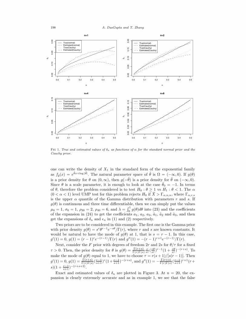
Numerical results very similar to the normal prior are seen for the Cauchy case.From Figure 1, we see that for each of the normal and the Cauchy prior, only about
1% of those null hypotheses a frequentist rejects with a p-value of less than 5% are
true. Indeed quite typically, δn < α for even very small values of n. This is discussedin greater detail in Section 4.5. This finding seems to be quite interesting.
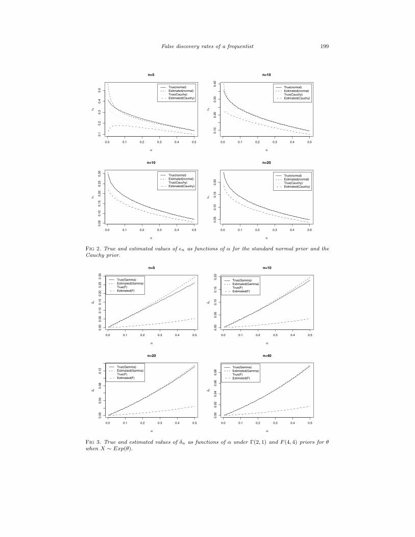
The true values of δn and ǫn are computed by taking an average of the lowerand the upper Riemann sums in An, An, Bn and Bn with the exact formulae forthe standard normal pdf. The accuracy of the expansion for δn is remarkable, ascan be seen in Figure 1. Even for n = 4, the true value of δn is almost identical tothe expansion in (1). The accuracy of the expansion for ǫn is very good (even if itis not as good as that for δn). For n = 20, the true value of ǫn is almost identicalto the expansion in (2).
Example 2. Let X1, · · · , Xn be iid Exp(θ), with density fθ(x) = θe−θx if x > 0.Clearly, µ(θ) = 1/θ, σ2(θ) = 1/θ2, ρ3(θ) = 2 and ρ4(θ) = 6. Let θ = −θ. Then,
198 A. DasGupta and T. Zhang
0.0 0.1 0.2 0.3 0.4 0.5
0.0
00
.10
0.2
00
.30
n=1
n
True(normal)Estimated(normal)True(Cauchy)Estimated(Cauchy)
0.0 0.1 0.2 0.3 0.4 0.5
0.0
00
.05
0.1
00
.15
0.2
0
n=2
n
True(normal)Estimated(normal)True(Cauchy)Estimated(Cauchy)
0.0 0.1 0.2 0.3 0.4 0.5
0.0
00.0
50
.10
0.1
5
n=4
n
True(normal)Estimated(normal)True(Cauchy)Estimated(Cauchy)
0.0 0.1 0.2 0.3 0.4 0.5
0.0
00.0
20.0
40.0
60
.08
0.1
0
n=8
n
True(normal)Estimated(normal)True(Cauchy)Estimated(Cauchy)
Fig 1. True and estimated values of δn as functions of α for the standard normal prior and the
Cauchy prior.
one can write the density of X1 in the standard form of the exponential family
as fθ(x) = eθx+log |θ|. The natural parameter space of θ is Ω = (−∞, 0). If g(θ)
is a prior density for θ on (0,∞), then g(−θ) is a prior density for θ on (−∞, 0).Since θ is a scale parameter, it is enough to look at the case θ0 = −1. In termsof θ, therefore the problem considered is to test H0 : θ ≥ 1 vs H1 : θ < 1. The α(0 < α < 1) level UMP test for this problem rejects H0 if X > Γα,n,n, where Γα,r,s
is the upper α quantile of the Gamma distribution with parameters r and s. Ifg(θ) is continuous and three time differentiable, then we can simply put the values
µ0 = 1, σ0 = 1, ρ30 = 2, ρ40 = 6, and λ =∫ 1
0g(θ)dθ into (23) and the coefficients
of the expansion in (24) to get the coefficients a1, a2, a3, a1, a2 and a3, and thenget the expansions of δn and ǫn in (1) and (2) respectively.
Two priors are to be considered in this example. The first one is the Gamma priorwith prior density g(θ) = srθr−1e−sθ/Γ(r), where r and s are known constants. Itwould be natural to have the mode of g(θ) at 1, that is s = r − 1. In this case,g′(1) = 0, g(1) = (r − 1)re−(r−1)/Γ(r) and g′′(1) = −(r − 1)r+1e−(r−1)/Γ(r).
Next, consider the F prior with degrees of freedom 2r and 2s for θ/τ for a fixed
τ > 0. Then, the prior density for θ is g(θ) = Γ(r+s)Γ(r)Γ(s)
rsτ ( rθ
sτ )r−1(1 + rθsτ )−(r+s). To
make the mode of g(θ) equal to 1, we have to choose τ = r(s + 1)/[s(r − 1)]. Then
g′(1) = 0, g(1) = Γ(r+s)Γ(r)Γ(s) (
r−1s+1 )r(1+ r−1
s+1 )−(r+s), and g′′(1) = − Γ(r+s)Γ(r)Γ(s) (
r−1s+1 )r+1(r+
s)(1 + r−1s+1 )−(r+s+2).
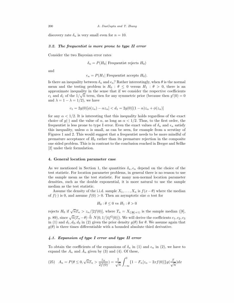
Exact and estimated values of δn are plotted in Figure 3. At n = 20, the ex-pansion is clearly extremely accurate and as in example 1, we see that the false
False discovery rates of a frequentist 199
0.0 0.1 0.2 0.3 0.4 0.5
0.1
0.2
0.3
0.4
0.5
n=5
n
True(normal)Estimated(normal)True(Cauchy)Estimated(Cauchy)
0.0 0.1 0.2 0.3 0.4 0.5
0.1
00
.20
0.3
00
.40
n=10
n
True(normal)Estimated(normal)True(Cauchy)Estimated(Cauchy)
0.0 0.1 0.2 0.3 0.4 0.5
0.0
50
.10
0.1
50
.20
0.2
50
.30
n=10
n
True(normal)Estimated(normal)True(Cauchy)Estimated(Cauchy)
0.0 0.1 0.2 0.3 0.4 0.5
0.0
50
.10
0.1
50
.20
n=20
n
True(normal)Estimated(normal)True(Cauchy)Estimated(Cauchy)
Fig 2. True and estimated values of ǫn as functions of α for the standard normal prior and the
Cauchy prior.
0.0 0.1 0.2 0.3 0.4 0.5
0.0
00
.05
0.1
00
.15
0.2
00
.25
0.3
0
n=5
n
True(Gamma)Estimated(Gamma)True(F)Estimated(F)
0.0 0.1 0.2 0.3 0.4 0.5
0.0
00
.05
0.1
00
.15
0.2
0
n=10
n
True(Gamma)Estimated(Gamma)True(F)Estimated(F)
0.0 0.1 0.2 0.3 0.4 0.5
0.0
00
.04
0.0
80
.12
n=20
n
True(Gamma)Estimated(Gamma)True(F)Estimated(F)
0.0 0.1 0.2 0.3 0.4 0.5
0.0
00
.02
0.0
40
.06
0.0
8
n=40
n
True(Gamma)Estimated(Gamma)True(F)Estimated(F)
Fig 3. True and estimated values of δn as functions of α under Γ(2, 1) and F (4, 4) priors for θ
when X ∼ Exp(θ).
200 A. DasGupta and T. Zhang
discovery rate δn is very small even for n = 10.
3.2. The frequentist is more prone to type II error
Consider the two Bayesian error rates
δn = P (H0| Frequentist rejects H0)
andǫn = P (H1| Frequentist accepts H0).
Is there an inequality between δn and ǫn? Rather interestingly, when θ is the normalmean and the testing problem is H0 : θ ≤ 0 versus H1 : θ > 0, there is anapproximate inequality in the sense that if we consider the respective coefficientsc1 and d1 of the 1/
√n term, then for any symmetric prior (because then g′(0) = 0
and λ = 1 − λ = 1/2), we have
c1 = 2g(0)[φ(zα) − αzα] < d1 = 2g(0)[(1 − α)zα + φ(zα)]
for any α < 1/2. It is interesting that this inequality holds regardless of the exactchoice of g(·) and the value of α, as long as α < 1/2. Thus, to the first order, thefrequentist is less prone to type I error. Even the exact values of δn and ǫn satisfythis inequality, unless α is small, as can be seen, for example from a scrutiny ofFigures 1 and 2. This would suggest that a frequentist needs to be more mindful ofpremature acceptance of H0 rather than its premature rejection in the compositeone sided problem. This is in contrast to the conclusion reached in Berger and Sellke[2] under their formulation.
4. General location parameter case
As we mentioned in Section 1, the quantities δn, ǫn depend on the choice of thetest statistic. For location parameter problems, in general there is no reason to usethe sample mean as the test statistic. For many non-normal location parameterdensities, such as the double exponential, it is more natural to use the samplemedian as the test statistic.
Assume the density of the i.i.d. sample X1, . . . , Xn is f(x− θ) where the medianof f(·) is 0, and assume f(0) > 0. Then an asymptotic size α test for
H0 : θ ≤ 0 vs H1 : θ > 0
rejects H0 if√
nTn > zα/[2f(0)], where Tn = X([ n
2]+1) is the sample median ([8],
p. 89), since√
n(Tn−θ)L⇒ N(0, 1/[4f2(0)]). We will derive the coefficients c1, c2, c3
in (1) and d1, d2, d3 in (2) given the prior density g(θ) for θ. We assume again thatg(θ) is three times differentiable with a bounded absolute third derivative.
4.1. Expansion of type I error and type II error
To obtain the coefficients of the expansions of δn in (1) and ǫn in (2), we have toexpand the An and An given by (3) and (4). Of these,
(25) An = P (θ ≤ 0,√
nTn >zα
2f(0)) =
1√n
∫ 0
−∞1 − Fn[zα − 2xf(0)]g(
x√n
)dx
False discovery rates of a frequentist 201
where Fn is the CDF of 2f(0)√
n(Tn − θ) if the true median is θ. Reiss [16] givesthe expansion of Fn as
Fn(t) = Φ(t) +φ(t)√
nR1(t) +
φ(t)
nR2(t) + rt,n,(26)
where, with x denoting the fractional part of a real x, R1(t) = f11t2 + f12, f11 =
f ′(0)/[4f2(0)], f12 = −(1 − 2n2 ), and R2(t) = f21t
5 + f22t3 + f23t, where f21 =
−[f ′(0)/f2(0)]2/32, f22 = 1/4+(1/2−n2 )[f ′(0)/(2f2(0))]+f ′′(0)/[24f3(0)], f23 =
1/4−(1−2n2 )2/2. The error term r1,t,n can be written as rt,n = φ(t)R3(t)/n3/2 +
O(n−2), where R3(t) is a polynomial.By letting y = 2xf(0) − zα in (25), we have
An =1
2f(0)√
n
∫ −zα
−∞Φ(y) − φ(y)√
nR1(−y) − φ(y)
nR2(−y) − r−y,n
(27)
× [g(0) + g′(0)y + zα
2f(0)√
n+
g′′(0)
2
(y + zα)2
4f2(0)n+
(y + zα)3
48f3(0)n3/2g(3)(y∗)]dy,
where y∗ is between 0 and (y + zα)/[2f(0)√
n].Hence, assuming supθ |g(3)(θ)| < ∞, on exact integration of each product of
functions in (27) and on collapsing the terms, we get
An =a1√n
+a2
n+
a3
n3/2+ O(n−2),(28)
where
a1 =g(0)
2f(0)[φ(zα) − αzα],(29)
a2 =g′(0)
8f2(0)[zαφ(zα) − α(z2
α + 1)] − g(0)
2f(0)f11[zαφ(zα) + α] + f12α(30)
and
a3 =g′′(0)
48f3(0)[(z2
α + 2)φ(zα) − α(z3α + 3zα)]
− g′(0)
4f2(0)f11[αzα − 2φ(zα)] + f12[αzα − φ(zα)]
− g(0)
2f(0)f21[(z
4α + 4z2
α + 8)φ(zα)] + f22[(z2α + 2)φ(zα)] + f23φ(zα).
(31)
We claim the error term in (28) is O(n−2). To prove this, we need to look at itsexact form, namely,
−O(n−2)
2f(0)
∫ −zα
−∞φ(y)R3(−y)g(θ0 +
y + zα
2f(0)√
n)dy + O(n−2)
∫ 0
−∞g(θ0 + y)dy.
Since g(θ) is absolutely uniformly bounded, the first term above is bounded byO(n−2). The second term is O(n−2) obviously. This shows that the error term in(28) is O(n−2).
202 A. DasGupta and T. Zhang
As regards An given by (4), one can similarly obtain
An =P (θ > 0,√
Tn ≤ zα
2f(0)) =
1√n
∫ ∞
0
Fn[zα − 2f(0)x]g(x√n
)dx
=a1√n
+a2
n+
a3
n32
+ O(n−2),
(32)
where y∗ is between 0 and (zα−y)/[2f(0)√
n], a1 = [g(0)/(2f(0))][(1−α)zα+φ(zα)],a2 = [g′(0)/(8f2(0))][(1 − α)(z2
α + 1) + zαφ(zα)] + [g(0)/(2f(0))]f11[(1 − α) −zαφ(zα)] + f12(1−α), a3 = [g′′(0)/(48f3(0))][(z2
α +2)φ(zα)+ (1−α)(z3α + 3zα)] +
[g′(0)/(4f2(0))]f11[(1−α)zα +2φ(zα)]+ f12[(1−α)zα +φ(zα)]− [g(0)/(2f(0))]×f21[(z
4α + 4z2
α + 8)φ(zα)] + f22[(z2α + 2)φ(zα)] + f23φ(zα). The error term in (32)
is still O(n−2) and this proof is omitted.
Therefore, we have the the expansions of Bn given by (5) Bn = λ−b1/√
n−b2/n−b3/n3/2 + O(n−2) where λ =
∫∞0
g(θ)dθ as before, b1 = a1 − a1 = zαg(0)/[2f(0)],b2 = a2 − a2 = g′(0)(z2
α + 1)/[8f2(0)] + g(0)(f11 + f12)/[2f(0)], b3 = a3 − a3 =g′′(0)(z3
α + 3zα)/[48f3(0)] + zαg′(0)(f11 + f12)/[4f2(0)]. Substituting a1, a2, a3, a1,a2, a3, b1, b2 and b3 into (7), we get the expansions of δn and ǫn for the generallocation parameter case given by (1) and (2).
4.2. Testing with mean vs. testing with median
Suppose X1, . . . , Xn are i.i.d. observations from a N(θ, 1) density and the statis-tician tests H0 : θ ≤ 0 vs. H1 : θ > 0 by using either the sample mean X orthe median Tn. It is natural to ask the choice of which statistic makes him morevulnerable to false discoveries. We can look at both false discovery rates δn and ǫn
to make this comparison, but we will do so only for the type I error rate δn here.
We assume for algebraic simplicity that g is symmetric, and so g′(0) = 0 andλ = 1/2. Also, to keep track of the two statistics, we will denote the coefficientsc1, c2 by c1,X , c1,Tn
, c2,X and c2,Tnrespectively. Then from our expansions in section
3.1 and section 4.1, it follows that
c1,Tn− c1,X = g(0)(φ(zα) − αzα)(
√2π − 2) = a(say),
and
c2,Tn− c2,X = g2(0)zα(φ(zα) − αzα)(2π − 4) − g(0)
√2πf12α
≥ g2(0)zα(φ(zα) − αzα)(2π − 4) = b(say) as f12 ≤ 0.
Hence, there exist positive constants a, b such that lim infn→∞√
n(√
n(δn,Tn−
δn,X)−a) ≥ b, i.e., the statistician is more vulnerable to a type I false discovery byusing the sample median as his test statistic. Now, of course, as a point estimator,Tn is less efficient than the mean X in the normal case. Thus, the statistician ismore vulnerable to a false discovery if he uses the less efficient point estimator ashis test statistic. We find this neat connection between efficiency in estimation andfalse discovery rates in testing to be interesting. Of course, similar connections arewell known in the literature on Pitman efficiencies of tests; see, e.g., van der Vaart([24], p. 201).
False discovery rates of a frequentist 203
4.3. Examples
In this subsection, we are going to study the exact values and the expansions forδn and ǫn in two examples. One example is f(x) = φ(x) and g(θ) = φ(θ); for theother example, f and g are both densities of the standard Cauchy. We will referto them as normal-normal and Cauchy-Cauchy for convenience of reference. Thepurpose of the first example is comparison with the normal-normal case when thetest statistic was the sample mean (Example 2 in Section 3); the second exampleis an independent natural example.
For exact numerical evaluation of δn and ǫn, the following formulae are necessary.The pdf of the standardized median 2f(0)
√n(Tn − θ) is
(33) fn(t) =
√n(
n−1[ n
2]−1
)
2f(0)f(
t
2f(0)√
n)F [ n
2]−1(
t
2f(0)√
n)(1 − F (
t
2f(0)√
n))n−[ n
2].
We are now ready to present our examples.
Example 3. Suppose X1, X2, . . . , Xn are i.i.d. N(θ, 1) and g(θ) = φ(θ). Then,g(0) = f(0) = 1/
√2π, g′(0) = f ′(0) = 0 and g′′(0) = f ′′(0) = −1/
√2π. Then,
we have f11 = 0, f12 = −(1 − 2n2 ), f21 = 0, f22 = 1/4 − π/12 and f23 =
1/4 − (1/2 − n2 )2. Plugging these values for f11, f12, f21, f22, f23 into (29), (30),
(31) and (7), we obtain the expansions for δn, and similarly for ǫn in the normal-normal case.
Next we consider the Cauchy-Cauchy case, i.e., X1, . . . , Xn are i.i.d. with densityfunction f(x) = 1/π[1 + (x − θ)2] and g(θ) = 1/[π(1 + θ2)]. Then, f(0) = 1/π,f ′(0) = 0 and f ′′(0) = −2/π. Therefore, f11 = 0, f12 = −(1 − 2n
2 ), f21 =0, f22 = 1/4 − π2/12, and f23 = 1/4 − (1/2 − n
2 )2. Plugging these values forf11, f12, f21, f22, f23 in (29), (30), (31), we obtain the expansions for δn, and similarlyfor ǫn in the Cauchy-Cauchy case.
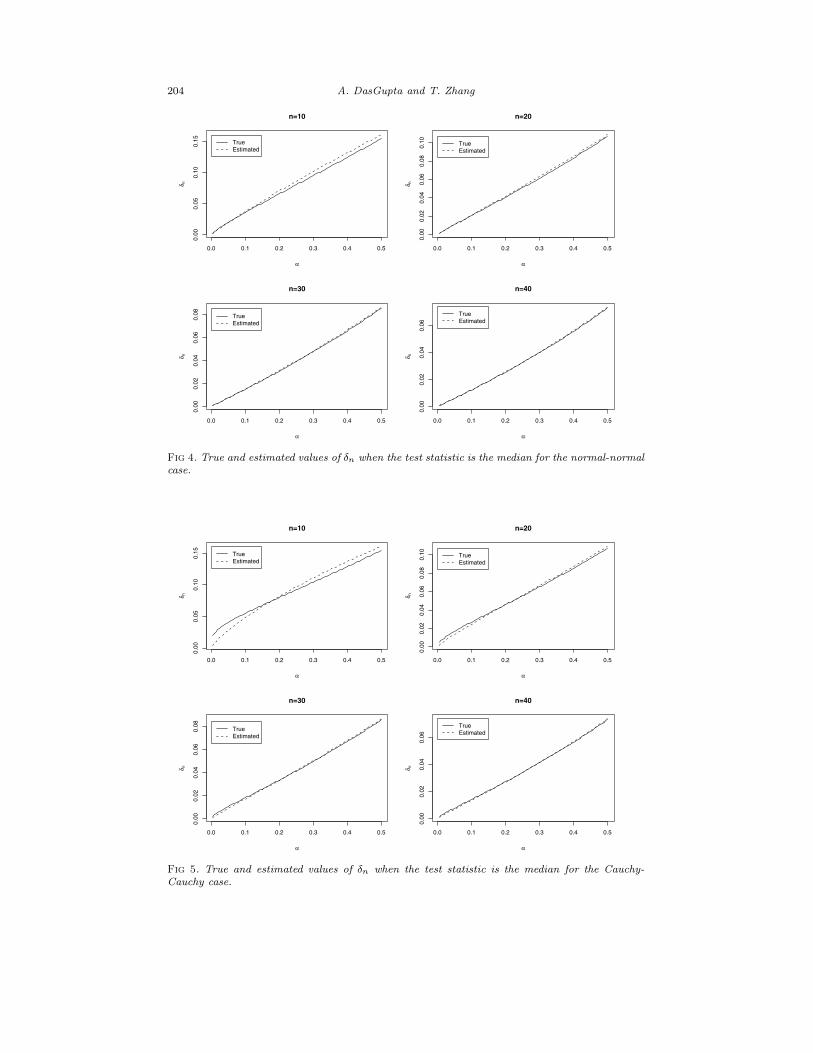
The true and estimated values of δn for selected n are given in Figure 4 andFigure 5. As before, the true values of δn and ǫ are computed by taking an averageof the lower and the upper Riemann sums in An, An, Bn and Bn with the exactformulae for fn as in (33). It can be seen that the two values are almost identicalwhen n = 30. By comparison with Figure 1, we see that the expansion for themedian is not as precise as the expansion for the sample mean.
The most important thing we learn is how small δn is for very moderate valuesof n. For example, in Figure 4, δn is only about 0.01 if α = 0.05, when n = 20.Again we see that even though we have changed the test statistic to the median,the frequentist’s false discovery rate is very small and, in particular, smaller thanα. More about this is said in Sections 4.4 and 4.5.
4.4. Spiky priors and false discovery rates
We commented in Section 4.1 that if the prior density g(θ0) is large, it increasesthe leading term in the expansion for δn (and also ǫn) and so it can be expectedthat spiky priors cause higher false discovery rates. In this section, we address theeffect of spiky and flat priors a little more formally.
Consider the general testing problem H0 : θ ≤ θ0 vs H1 : θ > θ0, where thenatural parameter space Ω = (θ, θ).
Suppose the α (0 < α < 1) level test rejects H0 if Tn ∈ C, where Tn is the teststatistic. Let Pn(θ) = Pθ(Tn ∈ C). Let g(θ) be any fixed density function for θ and
204 A. DasGupta and T. Zhang
0.0 0.1 0.2 0.3 0.4 0.5
0.0
00
.05
0.1
00
.15
n=10
n
TrueEstimated
0.0 0.1 0.2 0.3 0.4 0.5
0.0
00
.02
0.0
40
.06
0.0
80
.10
n=20
n
TrueEstimated
0.0 0.1 0.2 0.3 0.4 0.5
0.0
00
.02
0.0
40
.06
0.0
8
n=30
n
TrueEstimated
0.0 0.1 0.2 0.3 0.4 0.50
.00
0.0
20
.04
0.0
6
n=40
n
TrueEstimated
Fig 4. True and estimated values of δn when the test statistic is the median for the normal-normal
case.
0.0 0.1 0.2 0.3 0.4 0.5
0.0
00
.05
0.1
00
.15
n=10
n
TrueEstimated
0.0 0.1 0.2 0.3 0.4 0.5
0.0
00
.02
0.0
40
.06
0.0
80
.10
n=20
n
TrueEstimated
0.0 0.1 0.2 0.3 0.4 0.5
0.0
00
.02
0.0
40
.06
0.0
8
n=30
n
TrueEstimated
0.0 0.1 0.2 0.3 0.4 0.5
0.0
00
.02
0.0
40
.06
n=40
n
TrueEstimated
Fig 5. True and estimated values of δn when the test statistic is the median for the Cauchy-
Cauchy case.
False discovery rates of a frequentist 205
let gτ (θ) = g(θ/τ)/τ , τ > 0. Then gτ (θ) is spiky at 0 for small τ and gτ (θ) is flatfor large τ . When θ0 = 0, under the prior gτ (θ),
δn(τ) = P (θ ≤ 0|Tn ∈ C) =
∫ 0
θ/τPn(τy)g(y)dy
∫ θ/τ
θ/τ Pn(τy)g(y)dy,(34)
and
ǫn(τ) = P (θ > 0|Tn 6∈ C) =
∫ 0
θ/τ[1 − Pn(τy)]g(y)dy
∫ θ/τ
θ/τ[1 − Pn(τy)]g(y)dy
.(35)
Let as before λ =∫ 0
−∞ g(θ)dθ, the numerator and denominator of (34) be denotedby An(τ) and Bn(τ) and the numerator and denominator of (35) be denoted byAn(τ) and Bn(τ). Then, we have the following results.
Proposition 1. If P−n (θ0) = limθ→θ0− Pn(θ) and P+
n (θ0) = limθ→θ0+ Pn(θ) both
exist and are positive, then
limτ→0
δn(τ) =λP−
n (0)
λP−n (0) + (1 − λ)P+
n (0)(36)
and
limτ→0
ǫn(τ) =(1 − λ)[1 − P+
n (0)]
λ[1 − P−n (0)] + (1 − λ)[1 − P+
n (0)].(37)
Proof. Because 0 ≤ Pn(τy) ≤ 1 for all y, by simply applying the Lebesgue Domi-nated Convergence Theorem, limτ→0 An(τ) = λP−
n (0), limτ→0 Bn(τ) = λP−n (0) +
(1−λ)P+n (0), limτ→0 An(τ) = (1−λ)[1−P+
n (0)] and limτ→0 Bn(τ) = λ[1−P−n (0)]+
(1 − λ)[1 − P+n (0)]. Substituting in (34) and (35), we get (36) and (37).
Corollary 1. If 0 < λ < 1, limτ→∞ Pn(τy) = 0 for all y < 0, limτ→∞ Pn(τy) = 1for all y > 0, then limτ→∞ δn(τ) = limτ→∞ ǫn(τ) = 0.
Proof. Immediate from (36) and (37).
It can be seen that P−n (0) = P+
n (0) in most testing problems when the teststatistic Tn has a continuous power function. It is true for all the problems wediscussed in Sections 3 and 4. If moreover g(θ) > 0 for all θ, then 0 < λ < 1.As a consequence, limτ→0 δn(τ) = λ, limτ→0 ǫn(τ) = 1 − λ, and limτ→∞ δn(τ) =limτ→∞ ǫn(τ) = 0. If θ is a location parameter, θ0 = 0 and g(θ) is symmetric about0, then limτ→0 δn(τ) = limτ→0 ǫn(τ) = 1/2.
In other words, the false discovery rates are very small for any n for flat priorsand roughly 50% for any n for very spiky symmetric priors. This is a qualitativelyinformative observation.
4.5. Pre-experimental promise and post-experimental honesty
We noticed in our example in Section 4.4 that for quite small values of n, thepost-experimental error rate δn was smaller than the pre-experimental assurance,namely α. For any given prior g, this is true for all large n; but clearly we cannotachieve this uniformly over all g, or even large classes of g. In order to remain
206 A. DasGupta and T. Zhang
0.0
510
15
20
Normal
log( )
n
o
o
o
o
o
o
o
o
o
o
o
o
o
o
o
o
o
o
o
o
x
x
x
x
x
x
x
x
x
x
x
x
x
x
x
x
x
x
x
x =0.05
=0.01
o
x
0 1 2 3 4 5
510
15
Cauchy
log( )
no
o
o
o
o
o
o
o
o
o
x
x
x
x
x
x
x
x
x
x =0.05
=0.01ox
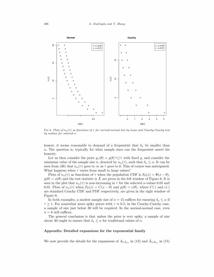
Fig 6. Plots of nα(τ) as functions of τ for normal-normal test by mean and Cauchy-Cauchy test
by median for selected α.
honest, it seems reasonable to demand of a frequentist that δn be smaller thanα. The question is, typically for what sample sizes can the frequentist assert hishonesty.
Let us then consider the prior gτ (θ) = g(θ/τ)/τ with fixed g, and consider theminimum value of the sample size n, denoted by nα(τ), such that δn ≤ α. It can beseen from (36) that nα(τ) goes to ∞ as τ goes to 0. This of course was anticipated.What happens when τ varies from small to large values?
Plots of nα(τ) as functions of τ when the population CDF is Fθ(x) = Φ(x − θ),g(θ) = φ(θ) and the test statistic is X are given in the left window of Figure 6. It isseen in the plot that nα(τ) is non-increasing in τ for the selected α-values 0.05 and0.01. Plots of nα(τ) when Fθ(x) = C(x − θ) and g(θ) = c(θ), where C(·) and c(·)are standard Cauchy CDF and PDF respectively, are given in the right window ofFigure 6.
In both examples, a modest sample size of n = 15 suffices for ensuring δn ≤ α ifτ ≥ 1. For somewhat more spiky priors with τ ≈ 0.5, in the Cauchy-Cauchy case,a sample of size just below 30 will be required. In the normal-normal case, evenn = 8 still suffices.
The general conclusion is that unless the prior is very spiky, a sample of sizeabout 30 ought to ensure that δn ≤ α for traditional values of α.
Appendix: Detailed expansions for the exponential family
We now provide the details for the expansions of An,θ1nin (13) and An,θ2n
in (15)
False discovery rates of a frequentist 207
and we also prove that Rn,θ1nin (14) and Rn,θ2n
in (16) are smaller order terms.Suppose g(θ) is a three times differentiable proper prior for θ. The expansions are
considered for those θ0 so that the exponential family density has a positive varianceat θ0. Then, we can find two values θ1 and θ2 such that θ < θ1 < θ0 < θ2 < θand the minimum value of σ2(θ) is positive when θ1 ≤ θ ≤ θ2. That is if we letm0 = minθ1<θ<θ2
σ2(θ), then m0 > 0. Since σ2(θ), ki(θ), ρi(θ) and g(3)(θ) are allcontinuous in θ, each of them is uniformly bounded in absolute value for θ ∈ [θ1, θ2].We denote M0 as the common upper bound of the absolute values of σ2(θ), κi(θ)(i = 3, 4, 5), ρi(θ) (i = 3, 4, 5), g(θ), g′(θ), g′′(θ) and g(3)(θ).
In the rest of this section, we denote θ1n = θ0 + (θ1 − θ0)/n1/3, θ2n = θ0 + (θ2 −θ0)/n1/3, x1 = σ0
√n(θ1 − θ0) − zα, x2 = σ0
√n(θ2 − θ0) − zα, x1n = σ0
√n(θ1n −
θ0)− zα and x2n = σ0√
n(θ1n − θ0)− zα. As in (13), (14), (15) and (16), we defineAn,θ1n
= P (θ1n ≤ θ ≤ θ0, X ∈ C), Rn,θ1n= An − An,θ1n
, An,θ2n= P (θ0 < θ ≤
θ2n, X 6∈ C) and Rn,θ2n= An − An,θ2n
, where An and An are given by (3) and (4)
respectively. We write Bn,θ1= P (θ ≥ θ1n, X ∈ C) and Bn,θ2
= P (θ ≤ θ2n, X 6∈ C).
Then, one can also see that Rn,θ1n= Bn − Bn,θ1
and Rn,θ2n= Bn − Bn,θ2
from
definition, where Bn and Bn are given by (5) and (6) respectively.The following Proposition and Corollary claim that Rn,θ1n
and Rn,θ2nare the
smaller order terms. Therefore, the coefficients of the expansions of An and An areexactly the same as those of An,θ1n
and An,θ2n.
Proposition 2. Let θ1,τ,n = θ0 +(θ1−θ0)/nτ and θ2,τ,n = θ0 +(θ2−θ0)/nτ . If 0 ≤τ < 1/2, then for any ℓ < ∞, limn→∞ nlβn(θ1,τ,n) = limn→∞ nl[1− βn(θ2,τ,n)] = 0.
Proof. A proof of this can be obtained by simply using Markov’s inequality. Weomit it.
Corollary 2. For any l > 0, limn→∞ nlRn,θ1n= limn→∞ nlRn,θ2n
= 0.
Proof. Since βn(θ) is nondecreasing in θ, we have
nlRn,θ1n= nl
∫ θ1n
θ
βn(θ)g(θ)dθ ≤ nlβn(θ1,1/3,n)
∫ θ1n
θ
g(θ)dθ ≤ nlβn(θ1,1/3,n)
and similarly nlRn,θ2n≤ nl[1 − βn(θ2,1/3,n)]. The conclusion is drawn by taking
τ = 1/3 in Proposition 2.
In the rest of this section, we will only derive the expansion of An,θ1nin detail
since the expansion of An,θ2nis obtained exactly similarly.
Using the transformation x = σ0√
n(θ − θ0) − zα in the following integral, wehave
An,θ1n=
1
σ0√
n
∫ −zα
x1n
βn(θ0 +x + zα
σ0√
n)g(θ0 +
x + zα
σ0√
n)dx.(38)
Note that
βn(θ0 +x + zα
σ0√
n) = Pθ0+
x+zα
σ0√
n
(
√n
X − µ(θ0 + x+zα
σ0
√n)
σ(θ0 + x+zα
σ0
√n)
≥ kθ0,x,n
)
,(39)
where
kθ0,x,n =
[
√n
µ0 − µ(θ0 + x+zα
σ0
√n)
σ0+ kθ0,n
]
σ0
σ(θ0 + x+zα
σ0
√n).(40)
208 A. DasGupta and T. Zhang
We obtain the coefficients of the expansions of An,θ1nin the following steps:
1. The expansion of g(θ0 + x+zα
σ0
√n) for any fixed x ∈ [x1n,−zα] is obtained by
using Taylor expansions.2. The expansion of kθ0,x,n for any fixed x ∈ [x1n,−zα] is obtained by jointly
considering the Cornish-Fisher expansion of kθ0,n, the Taylor expansion of√n[µ0 − µ(θ0 + x+zα
σ0
√n)]/σ0 and the Taylor expansion of σ0/σ(θ0 + x+zα
σ0
√n).
3. Write the CDF of X in the form of Pθ[√
n X−µ(θ)σ(θ) ≤ u]. Formally substitute
θ = θ0 + x+zα
σ0
√n
and u = kθ0,x,n in the Edgeworth expansion of the CDF of
X. An expansion of βn(θ0 + x+zα
σ0
√n) is obtained by combining it with Taylor
expansions for a number of relevant functions (see (47)).4. The expansion of An,θ1n
is obtained by considering the product of the expan-
sions of g(θ0 + x+zα
σ0
√n) and βn(θ0 + x+zα
σ0
√n) under the integral sign.
5. Finally prove that all the error terms in Steps 1, 2, 3 and 4 are smaller orderterms.
We give the expansions in steps 1, 2, 3 and 4 in detail. For the error term studyin step 5, we omit the details due to the considerably tedious algebra.
Step 1: The expansion of g(θ0 + x+zα√n
) is easily obtained by using a Taylor
expansion:
g(θ0 +x + zα
σ0√
n) = g(θ0) + g′(θ0)
x + zα
σ0√
n+
g′′(θ0)
2
(x + zα)2
σ20n
+ rg,x,n.(41)
where rg,x,n is the error term.
Step 2: The Cornish–Fisher expansion of kθ0,n ([1], p. 117) is given by
(42) kθ0,n = zα +(z2
α − 1)ρ30
6√
n+
1
n
[
(z3α − 3zα)ρ40
24− (2z3
α − 5zα)ρ230
36
]
+ r1,n,
where r1,n is the error term.The Taylor expansion of the first term inside the bracket of (40) is
− (x + zα) − ρ30(x + zα)2
2√
n− ρ40(x + zα)3
6n+ r2,x,n(43)
and the Taylor expansion of the term outside of the bracket of (40) is
1 − ρ30(x + zα)
2√
n+
1
n
(
3ρ230
8− ρ40
4
)
(x + zα)2 + r3,x,n,(44)
where r2,x,n and r3,x,n are error terms.
Plugging (42), (43) and (44) into (40), we get the expansion of kθ0,x,n below:
kθ0,x,n = −x +1√n
f1(x) +1
nf2(x) + r4,x,n,(45)
where r4,x,n is the error term, f1(x) = f11x + f10 and f2(x) = f23x3 + f22x
2 +f21x + f20, and the coefficients for f1(x) and f2(x) are f10 = −(2z2
α + 1)ρ30/6,f11 = −zαρ30/2, f20 = (z3
α+2zα)ρ230/9−(z3
α+zα)ρ40/8, f21 = (7z2α/24+1/12)ρ2
30−z2
αρ40/4, f22 = 0, f23 = ρ40/12 − ρ230/8.
False discovery rates of a frequentist 209
Step 3: The Edgeworth expansion of the CDF of X is (Barndorff-Nielsen andCox ([1], p. 91) and Hall ([11], p. 45)) given below:
Pθ0+x+zα
σ0√
n
√n
X − µ(θ0 + x+zα
σ0
√n)
√
σ(θ0 + x+zα
σ0
√n)
≤ u
= Φ(u) − φ(u)√n
(u2 − 1)
6ρ3(θ0 +
x + zα
σ0√
n) − φ(u)
n[(u3 − 3u)
24(46)
× ρ4(θ0 +x + zα
σ0√
n) +
(u5 − 10u3 + 15u)
72ρ23(θ0 +
x + zα
σ0√
n)] + r5,n,
where r5,n is an error term. If we take µ = kθ0,x,n in (46), then the left side is
1 − βn(θ0 + x+zα√n
) and so
β(θ0 +x + zα
σ0√
n) = Φ(−kθ0,x,n) +
φ(kθ0,x,n)√n
(k2θ0,x,n − 1)
6ρ3(θ0 +
x + zα
σ0√
n)
+φ(kθ0,x,n)
n[(k3
θ0,x,n − 3kθ0,x,n)
24ρ4(θ0 +
x + zα
σ0√
n)
+(k5
θ0,x,n − 10k3θ0,x,n + 15kθ0,x,n)
72ρ23(θ0 +
x + zα
σ0√
n)] − r5,n.
(47)
Plug the Taylor expansion of ρ3(θ0 + x+zα
σ0
√n)
ρ3(θ0 +x + zα
σ0√
n) = ρ30 +
(x + zα)√n
(
ρ40 −3
2ρ230
)
+ r6,x,n(48)
in (47), where r6,x,n is an error term, and then consider the Taylor expansions of
the three terms related to kθ0,x,n in (47) and also use the expansion (45). On quitea bit of calculations, we obtain the following expansion:
βn(θ0 +x + zα
σ0√
n) = Φ(x) − φ(x)
[
f1(x)√n
+f2(x)
n
]
− xφ(x)
[
f1(x)√n
]2
+φ(x)(x2 − 1)
6√
n[ρ30 +
(x + zα)√n
(ρ40 −3
2ρ230)] +
ρ30
6nφ(x)(x3 − 3x)f1(x)
+φ(x)
n[(x3 − 3x)
24ρ40 +
(x5 − 10x3 + 15x)
72ρ230] + r7,x,n
=Φ(x) +φ(x)√
ng1(x) +
φ(x)
ng2(x) + r7,x,n,
(49)
where r7,x,n is an error term, g1(x) = g12x2+g11x+g10, g2(x) = g20+g21x+g22x
2+g23x
3 + g24x4 + g25x
5, and the coefficients of g1(x) and g2(x) are g12 = ρ30/6,g11 = zαρ30/2, g10 = z2
αρ30/3, g25 = ρ230/72, g24 = −zαρ2
30/12, g23 = ρ40/8 −13z2
αρ230/72−7ρ2
30/24, g22 = zαρ40/6−z3αρ2
30/6−zαρ230/12, g21 = (z2
α/4−7/24)ρ40−z4
αρ230/18− 13z2
αρ230/72 + 4ρ2
30/9, g20 = (z3α/8 − zα/24)ρ40 − (z3
α/9 − zα/36)ρ230.
Step 4: The expansion of An,θ1nis obtained by plugging the expansions of
β(θ0 + x+zα
σ0
√n) and g(θ0 + x+zα
σ0
√n). On careful calculations,
An,θ1n=
a1√n
+a2
n+
a3
n3/2+ r8,n,(50)
210 A. DasGupta and T. Zhang
where r8,n is an error term, a1 = (g(θ0)/σ0)[φ(zα) − αzα], a2 = ρ30g(θ0)[α +2αz2
α − 2zαφ(zα)]/(6σ0)− g′(θ0)[α(z2α + 1)− zαφ(zα)]/(2σ2
0), and a3 = [h11φ(zα) +αh12][(g
′′(θ0)/(6σ30)] + [h21φ(zα) + αh22][g
′(θ0)/σ20 ] + [h31φ(zα) + αh32][g(θ0)/σ0],
where h11 = z2α +2, h12 = −(z3
α +3zα), h21 = −(ρ30/3)(z2α +1), h22 = (ρ30/3)(z3
α +2zα), h31 = −z4
αρ230/36+ 4z2
αρ230/9 + ρ2
30/36− 5z2αρ40/24+ ρ40/24, h32 = −5z3
αρ230/
18 − 11zαρ230/36 + z3
αρ40/8 + zαρ40/8. These a1, a2 and a3 are the coefficients inthe expansion of (23).
The computation of the coefficients of the expansions of An,θ1nis now complete.
The rest of the work is to prove that all the error terms are smaller order terms. Butfirst we give the results for the expansion of An,θ2n
. The details for the expansions
of An,θ2nare omitted.
Expansion of An,θ2n: The expansion of An,θ2n
can be obtained similarly bysimply repeating all the steps for An,θ1n
. The results are given below:
An,θ2n=
a1√n
+a2
n+
a3
n3/2+ r9,n,(51)
where r9,n is an error term, a1 = g(θ0)[φ(zα) + (1 − α)zα]/σ0, a2 = g′(θ0)[(1 −α)(z2
α + 1) + zαφ(zα)]/(2σ20) − ρ30g(θ0)[(1 − α)/6 + (1 − α)z2
α/3 + zαφ(zα)/3]/σ0,and a3 = (g′′(θ0)/6σ3
0)[h11φ(zα)−(1−α)h12]−(g′(θ0)/σ20)[−h21φ(zα)+(1−α)h22]−
(g(θ0)/σ0)[−h31φ(zα) + (1 − α)h32], where h11, h12, h21, h22, h31 and h32 are thesame as defined in Step 3. These a1, a2 and a3 are the coefficients in the expansionof (24).
Remark. The coefficients of expansions of δn and ǫn are obtained by simply usingformula (7) with a1, a2 and a3 in (23) and also the coefficient a1, a2 and a3 in (24)respectively.
Step 5: (Error term study in the expansions of An,θ1n). We only give the main
steps because the details are too long. Recall from equation (38) that the rangeof integration corresponding to An,θ1n
is x1n ≤ x ≤ −zα. In this case, we havelimn→∞ x1n = ∞ and limn→∞ x1n/
√n = −zα. This fact is used when we prove the
error term is still a smaller order term when we move it out of the integral sign.(I) In (41), since g(3)(θ) is uniformly bounded in absolute values, rg,x,n is abso-
lutely bounded by a constant times n−3/2(x + zα)2
(II) From Barndorff-Nielsen and Cox [4.5, pp 117], the error term r1,n in (42) isabsolutely uniformly bounded by a constant times n−3/2.
(III) In (43) and (44), since ρi(θ) and κi(θ) (i = 3, 4, 5) are uniformly boundedin absolute values, the error term r2,x,n is absolutely bounded by a constanttimes n−3/2(x + zα)4 and the error term r3,x,n is absolutely bounded by aconstant times n−3/2(x + zα)3.
(IV) The exact form of the error term r4,x,n in (45) can be derived by consider-ing the higher order terms and their products in (42), (43) and (44) for thederivation of expression (45). The computation is complicated but straight-forward. However, still, since ρi(θ) and κi(θ) (i = 3, 4, 5) are uniformlybounded in absolute values, r4,x,n is absolutely bounded by n−3/2P1(|x|),where P1(|x|) is a seventh degree polynomial and its coefficients do not de-pend on n.
(V) Again, from Barndorff-Nielsen and Cox ([1], p. 91), the error term r5,n in(46) is absolutely bounded by a constant times n−3/2.
(VI) The error term r6,x,n in (48) is absolutely bounded by a constant timesn−1(x + zα)2 since ρi(θ) and κi(θ) (i = 3, 4, 5) are uniformly bounded inabsolute values.
False discovery rates of a frequentist 211
(VII) This is the critical step for the error term study since we need to provethat the error term is still a smaller order term when it is moved outof the integral in (50). We need to study the behaviors of Φ(−kθ0,x,n)
and φ(kθ0,x,n) as n → ∞ for all x ∈ [x1n,−zα] uniformly (see (49) indetail). This also explains why we choose θ1n = θ0 + (θ1 − θ0)/n1/3 andx1n = σ0
√n(θ1n − θ0) − zα at the beginning of this section, since in this
case |kθ0,x,n + x| is uniformly bounded by |x|/2 + 1 for a sufficiently largen. Then for sufficiently large n, the error term |r7,x,n| in (49) is uniformlybounded by |r7,x,n| ≤ φ(x/2 + 1)P2(|x|) where P2(|x|) is a twelveth degreepolynomial of |x| and its coefficients do not depend on n.
(VIII) Finally, we can show that the error term r8,n in (50) in O(n−2). This istedious but straightforward. It is proven by considering each of the tenterms in r8,n separately.
Remark. We can similarly prove that the error term r9,n in (51) corresponding to
An,θ2nis O(n−2). Since the steps are very similar, we do not mention them.
Acknowledgment
It is a pleasure to thank Michael Woodroofe for the numerous conversations wehad with him on the foundational questions and the technical aspects of this paper.This paper would never have been written without Michael’s association. We wouldalso like to thank two anonymous referees for their thoughtful remarks and JiayangSun for her editorial input. We thank Larry Brown for reading an earlier draft ofthe paper and for giving us important feedback and to Persi Diaconis for asking aquestion that helped us in interpreting the results.
References
[1] Barndorff-Nielsen, O. E. and Cox, D. R. (1989). Asymptotic Techniques
for Use in Statistics. Chapman and Hall, New York. MR1010226[2] Berger, J. and Sellke, T. (1987). Testing a point null hypothesis: the
irreconcilability of P values and evidence. J. Amer. Statist. Assoc. 82 112–122. MR0883340
[3] Benjamini, Y. and Hochberg, Y. (1995). Controlling the false discoveryrate: a practical and powerful approach to multiple testing. J. R. Stat. Soc.
Ser. B 57 289–300. MR1325392[4] Brown, L. (1986). Fundamentals of Statistical Exponential Families with Ap-
plications in Statistical Decision Theory. Institute of Mathematical Statistics,Hayward, CA. MR0882001
[5] Casella, G. and Berger, R. L. (1987). Reconciling Bayesian and frequen-tist evidence in the one-sided testing problem. J. Amer. Statist. Assoc. 82
106–111. MR0883339[6] Edwards, W., Lindman, H. and Savage, L. J. (1984). Bayesian statis-
tical inference for psychological research. Robustness of Bayesian analyses.Stud. Bayesian Econometrics Vol . 4. North-Holland, Amsterdam, pp. 1–62.MR0785366
[7] Efron, B. (2003). Robbins, empirical Bayes and microarrays. Ann. Statist.
31 366–378. MR1983533[8] Ferguson, T. (1996). A Course in Large Sample Theory. Chapman & Hall,
New York. MR1699953
212 A. DasGupta and T. Zhang
[9] Finner, H. and Roters, M. (2001). On the false discovery rate and expectedtype I errors. Biom. J. 43 985–1005. MR1878272
[10] Genovese, C. and Wasserman, L. (2002). Operating characteristics andextensions of the false discovery rate procedure. J. R. Stat. Soc. Ser. B 64
499–517. MR1924303[11] Hall, P. (1992). The Bootstrap and Edgeworth Expansion. Springer-Verlag,
New York. MR1145237[12] Hall, P. and Sellinger, B. (1986). Statistical significance: balancing evi-
dence against doubt. Australian J. Statist. 28 354–370.[13] Lehmann, E.L. (1986). Hypothesis Testing. Wiley, New York. MR0852406[14] Marden, J. (2000). Hypothesis testing: from p values to Bayes factors. J.
Amer. Statist. Assoc. 95 1316–1320. MR1825285[15] Petrov, V. V. (1995). Limit Theorems of Probability Theory: Sequences
of Independent Random Variables. Oxford University Press, Oxford, UK.MR1353441
[16] Reiss, R.D. (1976). Asymptotic expansion for sample quantiles, Ann. Prob.
4 249–258. MR0402868[17] Schervish, M. (1996). P values: what they are and what they are not. Amer-
ican Statistician 50 203–206. MR1422069[18] Sellke, T., Bayarri, M. J. and Berger, J. (2001). Calibration of p
values for testing precise null hypotheses. American Statistician 55 62–71.MR1818723
[19] Soric, B. (1989). Statistical “discoveries” and effect-size estimation. J. Amer.
Statist. Assoc. 84 608–610.[20] Storey, J. D. (2002). A direct approach to false discovery rate. J. R. Stat.
Soc. Ser. B 64 479–498. MR1924302[21] Storey, J. D. (2003). The positive false discovery rate: A Bayesian interpre-
tation and the p-value. Ann. Statist. 31 2013–2035. MR2036398[22] Storey, J. D., Taylor, J. E. and Siegmund, D. (2004). Strong control,
conservative point estimation and simultaneous conservative consistency offalse discovery rates: A unified approach. J. R. Stat. Soc. Ser. B 66 187–205.MR2035766
[23] Storey, J. D. and Tibshirani, R. (2003). Statistical significance forgenomewide studies. Proc. Natl. Acad. Sci. USA 16 9440–9445 (electronic).MR1994856
[24] van der Vaart, A.W. (1998). Asymptotic Statistics. Cambridge UniversityPress, Cambridge, UK. MR1652247


![On alpha-adic expansions in Pisot bases 1 - IRIFcf/publications/adic3.pdf · On alpha-adic expansions in Pisot bases1 ... Berth´e and Siegel [7] ... A computation cin A is a finite](https://static.fdocument.org/doc/165x107/5ac7f2f87f8b9a42358be311/on-alpha-adic-expansions-in-pisot-bases-1-irif-cfpublicationsadic3pdfon-alpha-adic.jpg)