Flavor anomalies and radiative neutrino mass with vector ...

Department of Physics, Central University of Karnataka

Flavor anomalies and radiative neutrinomass with vector leptoquark

P. S. Bhupal Dev, R. Mohanta, S. Patra and S. SahooBased on Phys. Rev. D 102 (2020), 095012

Dec 16, 2020

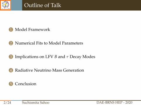
1 Model Framework

2 Numerical Fits to Model Parameters

3 Implications on LFV B and τ Decay Modes

4 Radiative Neutrino Mass Generation

5 Conclusion

Outline of Talk

2/24 Suchismita Sahoo DAE-BRNS HEP - 2020

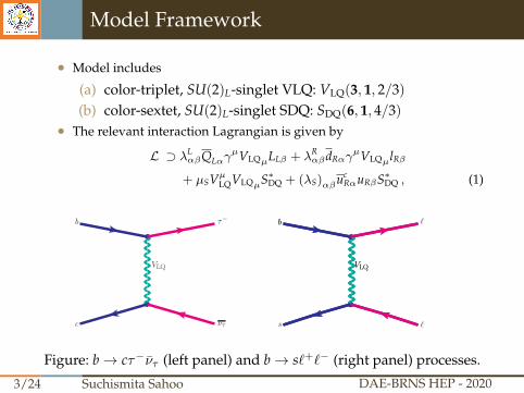
• Model includes

(a) color-triplet, SU(2)L-singlet VLQ: VLQ(3, 1, 2/3)

(b) color-sextet, SU(2)L-singlet SDQ: SDQ(6, 1, 4/3)

• The relevant interaction Lagrangian is given by

L ⊃ λLαβQLαγ

µVLQµLLβ + λRαβdRαγ

µVLQµlRβ

+ µSVµLQVLQµS∗DQ + (λS)αβuc

RαuRβS∗DQ , (1)

q′

ντ

b τ−

VLQ

cq′

q′

ℓ

b ℓ

VLQ

sq′

q′b

VLQ

q′

q′

q′

Figure: b→ cτ−ντ (left panel) and b→ s`+`− (right panel) processes.

Model Framework


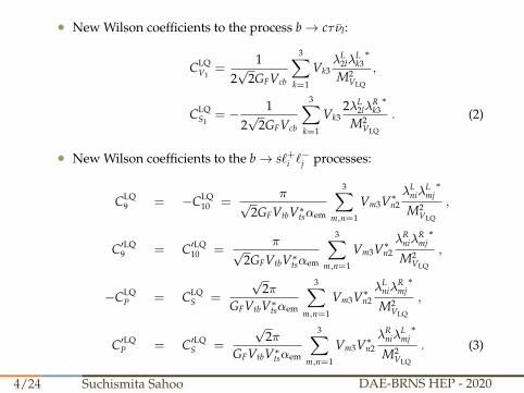
• New Wilson coefficients to the process b→ cτ νl:

CLQV1

=1

2√

2GFVcb

3∑k=1

Vk3λL

2lλLk3∗

M2VLQ

,

CLQS1

= − 12√

2GFVcb

3∑k=1

Vk32λL

2lλRk3∗

M2VLQ

. (2)

• New Wilson coefficients to the b→ s`+i `−j processes:

CLQ9 = −CLQ

10 =π√

2GFVtbV∗tsαem

3∑m,n=1

Vm3V∗n2λL

niλLmj∗

M2VLQ

,

C′LQ9 = C′LQ

10 =π√

2GFVtbV∗tsαem

3∑m,n=1

Vm3V∗n2λR

niλRmj∗

M2VLQ

,

−CLQP = CLQ

S =

√2π

GFVtbV∗tsαem

3∑m,n=1

Vm3V∗n2λL

niλRmj∗

M2VLQ

,

C′LQP = C′LQ

S =

√2π

GFVtbV∗tsαem

3∑m,n=1

Vm3V∗n2λR

niλLmj∗

M2VLQ

. (3)


We classify the new parameters into the following four scenarios:

• Scenario-I (S-I): Includes CLQV1

for b→ cτ ντ and CLQ9 = −CLQ

10 for b→ s``(contains only LL couplings).

• Scenario-II (S-II): Includes C′LQ9 = −C′LQ

10 for b→ s`` (involves only RRcouplings).

• Scenario-III (S-III): Includes CLQS1

for b→ cτ ντ and −CLQP = CLQ

S forb→ s`` (only LR couplings present).

• Scenario-IV (S-IV): Includes C′LQP = C′LQ

S for b→ s`` (involves only RLcouplings).


Observables used for numerical fit:

(a) b → sµµ

• RK & RK∗

RK =BR(B+ → K+µ+µ−)

BR(B+ → K+e+e−), RK∗ =

BR(B0 → K∗0µ+µ−)

BR(B0 → K∗0e+e−)(4)

• Br(Bs → µ+µ−), Br(B+,0 → K+,0(∗)µ+µ−) & Br(Bs → φµ+µ−)• AFB, FL, P1,2,3,P′4,5,6,8 & A3,4,5,6,7,8,9 of B(s) → K∗(φ)µµ

(b) b → cτ ντ

• RD, RD∗ & RJ/ψ

RD(∗) =BR(B→ D(∗)τ ντ )

BR(B→ D(∗)`ν`), RJ/ψ =

BR(B→ J/ψτντ )

BR(B→ J/ψ`ν`)(5)

• B+c → τ+ντ

(c) b → sτ+τ−

• Br(Bs → τ+τ−) & Br(B+ → K+τ+τ−)6/24 Suchismita Sahoo DAE-BRNS HEP - 2020

Observables not used in our analysis:

• b→ sν`ν` (B→ K(∗)ν`ν`)

• c→ s`ν` (D+s → `+ν`, D+ → K0`+ν`, D0 → K(∗)−`+ν`)

• Leptonic/semileptonic K(D) meson decay modes

• K0 − K0

(D0 −D0) mixing

• b→ uτντ (Bu → τντ )

• loop-level flavor-changing processes (Bs − Bs mixing, b→ sγ andb→ sνν, Z→ lilj)


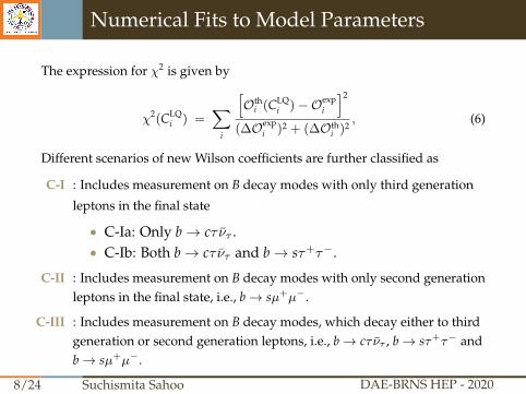
The expression for χ2 is given by

χ2(CLQi ) =

∑i

[Oth

i (CLQi )−Oexp

i

]2

(∆Oexpi )2 + (∆Oth

i )2, (6)

Different scenarios of new Wilson coefficients are further classified as

C-I : Includes measurement on B decay modes with only third generation

leptons in the final state

• C-Ia: Only b→ cτ ντ .• C-Ib: Both b→ cτ ντ and b→ sτ+τ−.

C-II : Includes measurement on B decay modes with only second generationleptons in the final state, i.e., b→ sµ+µ−.

C-III : Includes measurement on B decay modes, which decay either to thirdgeneration or second generation leptons, i.e., b→ cτ ντ , b→ sτ+τ− andb→ sµ+µ−.

Numerical Fits to Model Parameters


-2 -1 0 1 2

-2

-1

0

1

2

λ33

L

λ23

L

(a) C-Ia case of S-I

-2 -1 0 1 2

-2

-1

0

1

2

λ33

L

λ23

L

(b) C-Ib case of S-I

0.00 0.05 0.10 0.15

0.00

0.05

0.10

0.15

λ32

L

λ22

L

(c) C-II case of S-I

-2 -1 0 1 2

-2

-1

0

1

2

λ33

L

λ23

L

(d) C-III case of S-I inλL

33 − λL23 plane

0.00 0.05 0.10 0.15

0.00

0.05

0.10

0.15

λ32

L

λ22

L

(e) C-III case of S-I inλL

32 − λL22 plane


0.00 0.05 0.10 0.15 0.20 0.25 0.30 0.35

0.00

0.05

0.10

0.15

0.20

0.25

0.30

0.35

λ32

R

λ22

R

(f) C-II case of S-II

0.00 0.05 0.10 0.15 0.20 0.25

0.00

0.05

0.10

0.15

0.20

0.25

λ32

R

λ22

L

(g) C-II case of S-IV


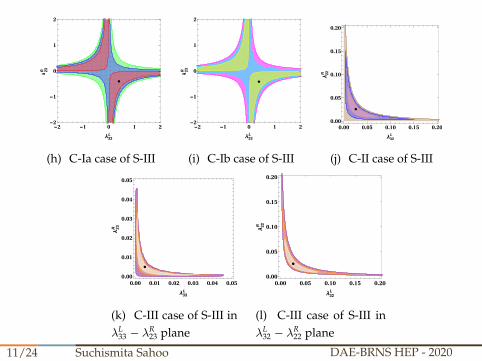
-2 -1 0 1 2-2

-1

0

1

2

λ33L

λ23R

(h) C-Ia case of S-III

-2 -1 0 1 2-2

-1

0

1

2

λ33L

λ23R

(i) C-Ib case of S-III

0.00 0.05 0.10 0.15 0.20

0.00

0.05

0.10

0.15

0.20

λ32

L

λ22

R

(j) C-II case of S-III

0.00 0.01 0.02 0.03 0.04 0.050.00

0.01

0.02

0.03

0.04

0.05

λ33L

λ23R

(k) C-III case of S-III inλL

33 − λR23 plane

0.00 0.05 0.10 0.15 0.20

0.00

0.05

0.10

0.15

0.20

λ32

L

λ22

R

(l) C-III case of S-III inλL

32 − λR22 plane


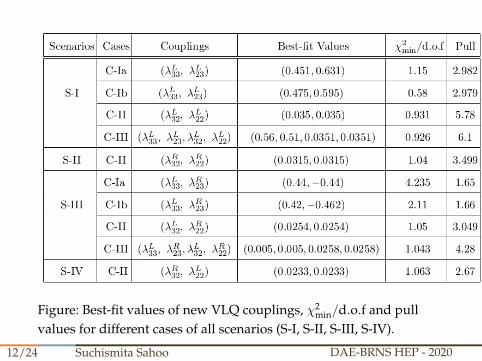
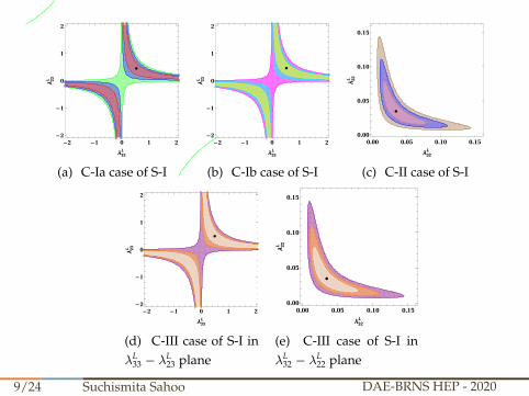
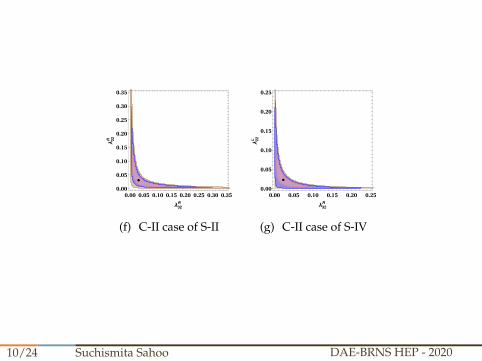
Figure: Best-fit values of new VLQ couplings, χ2min/d.o.f and pull

values for different cases of all scenarios (S-I, S-II, S-III, S-IV).


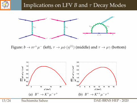
q′

τ+

b µ−

VLQ

sq′

q′

q′s

s

µ−

τ−

VLQ

q′

q′

d, s, bτ µ

VLQ VLQ

γ

q′

Figure: b→ sτ+µ− (left), τ → µφ (η(′)) (middle) and τ → µγ (bottom)

5 10 15 200.0

0.2

0.4

0.6

0.8

1.0

1.2

q2[Gev

2]

dBR

dq2

(B+→K

+μ-τ+)×107

(a) B+ → K+µ−τ+

4 6 8 10 12 14 16 180.0

0.5

1.0

1.5

2.0

2.5

3.0

q2[Gev

2]

dBR

dq2

(B+→K

*+μ-τ+)×107

(b) B+ → K∗+µ−τ+

Implications on LFV B and τ Decay Modes


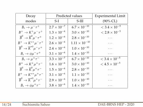
Decay Predicted values Experimental Limitmodes S-I S-III (90% CL)

Bs → µ−τ+ 2.7× 10−7 6.7× 10−10 < 3.4× 10−5

B+ → K+µ−τ+ 1.3× 10−6 3.0× 10−10 < 2.8× 10−5

B0 → K

0µ−τ+ 1.2× 10−6 2.8× 10−10 · · ·

B+ → K∗+µ−τ+ 2.6× 10−6 1.11× 10−10 · · ·B

0 → K∗0µ−τ+ 2.4× 10−6 1.0× 10−10 · · ·

Bs → φµ−τ+ 3.1× 10−6 1.4× 10−10 · · ·Bs → µ+τ− 3.3× 10−7 6.7× 10−10 < 3.4× 10−5

B+ → K+µ+τ− 1.6× 10−6 3.0× 10−10 < 4.5× 10−5

B0 → K

0µ+τ− 1.5× 10−6 2.8× 10−10 · · ·

B+ → K∗+µ+τ− 3.1× 10−6 1.1× 10−10 · · ·B

0 → K∗0µ+τ− 2.9× 10−6 1.0× 10−10 · · ·

Bs → φµ+τ− 3.8× 10−6 1.4× 10−10 · · ·


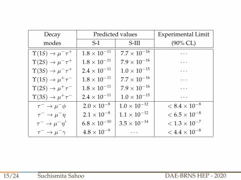
Decay Predicted values Experimental Limitmodes S-I S-III (90% CL)

Υ(1S)→ µ−τ+ 1.8× 10−11 7.7× 10−16 · · ·Υ(2S)→ µ−τ+ 1.8× 10−11 7.9× 10−16 · · ·Υ(3S)→ µ−τ+ 2.4× 10−11 1.0× 10−15 · · ·Υ(1S)→ µ+τ− 1.8× 10−11 7.7× 10−16 · · ·Υ(2S)→ µ+τ− 1.8× 10−11 7.9× 10−16 · · ·Υ(3S)→ µ+τ− 2.4× 10−11 1.0× 10−15 · · ·τ− → µ−φ 2.0× 10−8 1.0× 10−12 < 8.4× 10−8

τ− → µ−η 2.1× 10−8 1.1× 10−12 < 6.5× 10−8

τ− → µ−η′ 6.8× 10−10 3.5× 10−14 < 1.3× 10−7

τ− → µ−γ 4.8× 10−9 · · · < 4.4× 10−8


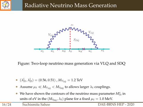
uL uR uR uL

a

νL νL

VLQVLQ

a

SDQ

λS

a

µS

Figure: Two-loop neutrino mass generation via VLQ and SDQ

• (λL33, λ

L23) = (0.56, 0.51) , MVLQ = 1.2 TeV

• Assume µS � MVLQ < MSDQ to allows larger λS couplings.

• We have shown the contours of the neutrino mass parameter Mν33 in

units of eV in the (MSDQ , λS) plane for a fixed µS = 1.0 MeV.

Radiative Neutrino Mass Generation


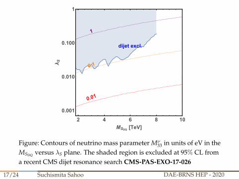
2 4 6 8 10

0.001

0.010

0.100

1

MSDQ [TeV]

λS

0.01

0.1

1

dijet excl.

Figure: Contours of neutrino mass parameter Mν33 in units of eV in the

MSDQ versus λS plane. The shaded region is excluded at 95% CL froma recent CMS dijet resonance search CMS-PAS-EXO-17-026


• To explain both CC b→ cτ ντ and NC b→ s`+`− transitions in a singleframwork, we have extended SM with vector LQ (3, 1, 2/3).

• We performed a global fit to constrain the NP parameters by using theobservables associated with b→ sµ−µ+(τ−τ+) and b→ cτ ντtransitions.

• We find that for a TeV-scale VLQ, only the LL-type couplings cansimultaneously explain both b→ s`+`− and b→ cτ ντ anomalies with aχ2

min/d.o.f. < 1.

• In addition, augmenting the VLQ model with a color-sextet SDQ canexplain the neutrino mass at two-loop level.

Thank you !!

Conclusion


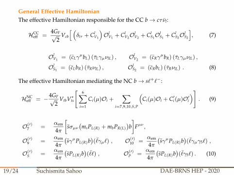
General Effective HamiltonianThe effective Hamiltonian responsible for the CC b→ cτ νl:

HCCeff =

4GF√2

Vcb

[ (δlτ + Cl

V1

)Ol

V1 + ClV2O

lV2 + Cl

S1OlS1 + Cl

S2OlS2

], (7)

OlV1 = (cLγ

µbL) (τLγµνlL) , OlV2 = (cRγ

µbR) (τLγµνlL) ,

OlS1 = (cLbR) (τRνlL) , Ol

S2 = (cRbL) (τRνlL) . (8)

The effective Hamiltonian mediating the NC b→ s`+`−:

HNCeff = −4GF√

2VtbV∗ts

[6∑

i=1

Ci(µ)Oi +∑

i=7,9,10,S,P

(Ci(µ)Oi + C′i (µ)O′i

)]. (9)

O(′)7 =

αem

4π

[sσµν

(msPL(R) + mbPR(L)

)b]

Fµν ,

O(′)9 =

αem

4π(sγµPL(R)b

)(¯γµ`) , O(′)

10 =αem

4π(sγµPL(R)b

)(¯γµγ5`) ,

O(′)S =

αem

4π(sPL(R)b

)(¯ ) , O(′)

P =αem

4π(sPL(R)b

)(¯γ5`) . (10)


• The current experimental value of the branching ratio of Bs → µ+µ−

process is

BR(B0s → µ+µ−) = (3.0± 0.4)× 10−9 , (11)

which is compatible with the SM prediction

BR(B0s → µ+µ−)SM = (3.65± 0.23)× 10−9 , (12)

at 1.6σ confidence level (CL).

• This channel has not been measured yet, but indirect constraints onBR(B+

c → τ+ντ ) . 30% have been imposed using the lifetime of Bc.

• In this sector, we consider the following two observables:BR(Bs → τ+τ−) < 6.8× 10−3 and BR(B+ → K+τ+τ−) < 2.2× 10−3 .


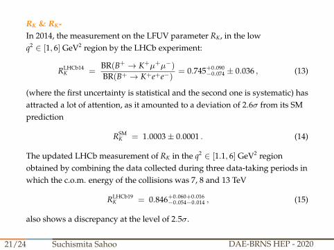
RK & RK∗

In 2014, the measurement on the LFUV parameter RK, in the lowq2 ∈ [1, 6] GeV2 region by the LHCb experiment:

RLHCb14K =

BR(B+ → K+µ+µ−)

BR(B+ → K+e+e−)= 0.745+0.090

−0.074 ± 0.036 , (13)

(where the first uncertainty is statistical and the second one is systematic) hasattracted a lot of attention, as it amounted to a deviation of 2.6σ from its SMprediction

RSMK = 1.0003± 0.0001 . (14)

The updated LHCb measurement of RK in the q2 ∈ [1.1, 6] GeV2 regionobtained by combining the data collected during three data-taking periods inwhich the c.o.m. energy of the collisions was 7, 8 and 13 TeV

RLHCb19K = 0.846+0.060+0.016

−0.054−0.014 , (15)

also shows a discrepancy at the level of 2.5σ.


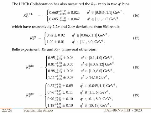
The LHCb Collaboration has also measured the RK∗ ratio in two q2 bins

RLHCbK∗ =

0.660+0.110−0.070 ± 0.024 q2 ∈ [0.045, 1.1] GeV2 ,

0.685+0.113−0.069 ± 0.047 q2 ∈ [1.1, 6.0] GeV2 .

(16)

which have respectively 2.2σ and 2.4σ deviations from SM results

RSMK∗ =

0.92± 0.02 q2 ∈ [0.045, 1.1] GeV2 ,

1.00± 0.01 q2 ∈ [1.1, 6.0] GeV2 .(17)

Belle experiment: RK and RK∗ in several other bins:

RBelleK =

0.95+0.27−0.24 ± 0.06 q2 ∈ [0.1, 4.0] GeV2 ,

0.81+0.28−0.23 ± 0.05 q2 ∈ [4.0, 8.12] GeV2 ,

0.98+0.27−0.23 ± 0.06 q2 ∈ [1.0, 6.0] GeV2 ,

1.11+0.29−0.26 ± 0.07 q2 > 14.18 GeV2 ,

(18)

RBelleK∗ =

0.52+0.36−0.26 ± 0.05 q2 ∈ [0.045, 1.1] GeV2 ,

0.96+0.45−0.29 ± 0.11 q2 ∈ [1.1, 6] GeV2 ,

0.90+0.27−0.21 ± 0.10 q2 ∈ [0.1, 8.0] GeV2 ,

1.18+0.52−0.32 ± 0.10 q2 ∈ [15, 19] GeV2 .

(19)


RD & RD∗

RExpD = 0.34± 0.027± 0.013 , (20)

RExpD∗ = 0.295± 0.011± 0.008 , (21)

induce a tension at the level of 3.08σ with the corresponding SM predictions

RSMD = 0.299± 0.003 , (22)

RSMD∗ = 0.258± 0.005 . (23)

Discrepancy of 1.7σ has also been observed between the experimentalmeasurement of

RExpJ/ψ =

BR(B→ J/ψτντ )

BR(B→ J/ψ`ν`)= 0.71± 0.17± 0.184 , (24)

and the corresponding SM prediction

RSMJ/ψ = 0.289± 0.01 . (25)


Neutrino mass: The two-loop contribution to light neutrino masses in theflavor basis is

Mναβ = 32λL

αjmujµS(λSI)jkmukλLkβ , (26)

where the finite part of the two-loop integral is given by

Ijk =

∫d4k

(2π)4

∫d4p

(2π)41(

k2 −m2uj

) 1(k2 −M2

VLQ

)× 1(

p2 −m2uk

) 1(p2 −M2

VLQ

) 1(p + k)2 −M2

SDQ

. (27)

Assuming that the VLQ and SDQ are much heavier than the SM quarks inthe loop, the loop function can be reduced to

Ijk ' I0 =1

(4π)4

1(max[MVLQ ,MSDQ ])2

π2

3I

(M2

SDQ

M2VLQ

), (28)

where I(x) has closed-form analytic expression in the following limits:

I(x) =

{1 + 3

π2

{(ln x)2 − 1

}for x� 1

1 for x� 1.(29)


Flavor anomalies and radiative neutrino mass with vector ...

Documents

Transcript of Flavor anomalies and radiative neutrino mass with vector ...