Numerical methods for multidimensional radiative...
43
Numerical methods for multidimensional radiative transfer * E. Meink¨ ohn 1,2 , G. Kanschat 1 , R. Rannacher 1,3 , and R. Wehrse 2,3 1 Institute of Applied Mathematics, University of Heidelberg, 2 Institute for Theoretical Astrophysics, University of Heidelberg, 3 Interdisciplinary Center for Scientific Computing, University of Heidelberg 1 Abstract This paper presents a continuous finite element method for solving the reso- nance line transfer problem in moving media. The algorithm is capable of deal- ing with three spatial dimensions, using hierarchically structured grids which are locally refined by means of duality-based a-posteriori error estimates. Ap- plication of the method to coherent isotropic scattering and complete redis- tribution gives a result of matrix structure which is discussed in the paper. The solution is obtained by way of an iterative procedure, which solves a succession of quasi-monochromatic radiative transfer problems. It is therefore immediately evident that any simulation of the extended frequency-dependent model requires a solution strategy for the elementary monochromatic transfer problem, which is fast as well as accurate. The present implementation is ap- plicable to arbitrary model configurations with optical depths up to 10 3 –10 4 . Additionally, a combination of a discontinuous finite element method with a superior preconditioning method is presented, which is designed to overcome the extremely poor convergence properties of the linear solver for optically thick and highly scattering media. The contents of this article is as follows: - Introduction - Overview: Numerical Methods - Monochromatic 3D Radiative Transfer - Polychromatic 3D Line Transfer - Test Calculations - Applications - Multi-Model Preconditioning - Summary - References ∗ This work has been supported by the German Research Foundation (DFG) through SFB 359 (Project C2).
Transcript of Numerical methods for multidimensional radiative...
Numerical methods for multidimensional
radiative transfer∗
E. Meinkohn1,2, G. Kanschat1, R. Rannacher1,3, and R. Wehrse2,3
1 Institute of Applied Mathematics, University of Heidelberg,2 Institute for Theoretical Astrophysics, University of Heidelberg,3 Interdisciplinary Center for Scientific Computing, University of Heidelberg
1 Abstract
This paper presents a continuous finite element method for solving the reso-nance line transfer problem in moving media. The algorithm is capable of deal-ing with three spatial dimensions, using hierarchically structured grids whichare locally refined by means of duality-based a-posteriori error estimates. Ap-plication of the method to coherent isotropic scattering and complete redis-tribution gives a result of matrix structure which is discussed in the paper.The solution is obtained by way of an iterative procedure, which solves asuccession of quasi-monochromatic radiative transfer problems. It is thereforeimmediately evident that any simulation of the extended frequency-dependentmodel requires a solution strategy for the elementary monochromatic transferproblem, which is fast as well as accurate. The present implementation is ap-plicable to arbitrary model configurations with optical depths up to 103–104.Additionally, a combination of a discontinuous finite element method with asuperior preconditioning method is presented, which is designed to overcomethe extremely poor convergence properties of the linear solver for opticallythick and highly scattering media. The contents of this article is as follows:
- Introduction- Overview: Numerical Methods- Monochromatic 3D Radiative Transfer- Polychromatic 3D Line Transfer- Test Calculations- Applications- Multi-Model Preconditioning- Summary- References
∗This work has been supported by the German Research Foundation (DFG)through SFB 359 (Project C2).
2 E. Meinkohn, G. Kanschat, R. Rannacher, and R. Wehrse
2 Introduction
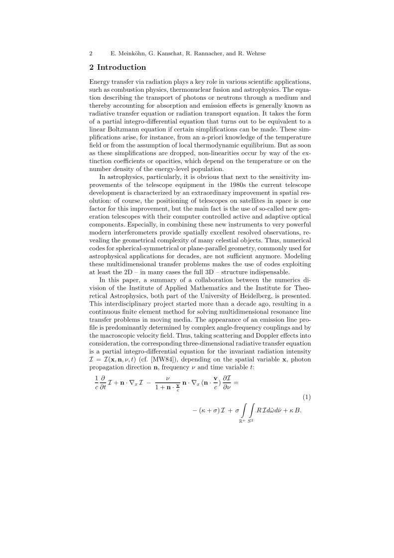
Energy transfer via radiation plays a key role in various scientific applications,such as combustion physics, thermonuclear fusion and astrophysics. The equa-tion describing the transport of photons or neutrons through a medium andthereby accounting for absorption and emission effects is generally known asradiative transfer equation or radiation transport equation. It takes the formof a partial integro-differential equation that turns out to be equivalent to alinear Boltzmann equation if certain simplifications can be made. These sim-plifications arise, for instance, from an a-priori knowledge of the temperaturefield or from the assumption of local thermodynamic equilibrium. But as soonas these simplifications are dropped, non-linearities occur by way of the ex-tinction coefficients or opacities, which depend on the temperature or on thenumber density of the energy-level population.
In astrophysics, particularly, it is obvious that next to the sensitivity im-provements of the telescope equipment in the 1980s the current telescopedevelopment is characterized by an extraordinary improvement in spatial res-olution: of course, the positioning of telescopes on satellites in space is onefactor for this improvement, but the main fact is the use of so-called new gen-eration telescopes with their computer controlled active and adaptive opticalcomponents. Especially, in combining these new instruments to very powerfulmodern interferometers provide spatially excellent resolved observations, re-vealing the geometrical complexity of many celestial objects. Thus, numericalcodes for spherical-symmetrical or plane-parallel geometry, commonly used forastrophysical applications for decades, are not sufficient anymore. Modelingthese multidimensional transfer problems makes the use of codes exploitingat least the 2D – in many cases the full 3D – structure indispensable.
In this paper, a summary of a collaboration between the numerics di-vision of the Institute of Applied Mathematics and the Institute for Theo-retical Astrophysics, both part of the University of Heidelberg, is presented.This interdisciplinary project started more than a decade ago, resulting in acontinuous finite element method for solving multidimensional resonance linetransfer problems in moving media. The appearance of an emission line pro-file is predominantly determined by complex angle-frequency couplings and bythe macroscopic velocity field. Thus, taking scattering and Doppler effects intoconsideration, the corresponding three-dimensional radiative transfer equationis a partial integro-differential equation for the invariant radiation intensityI = I(x,n, ν, t) (cf. [MW84]), depending on the spatial variable x, photonpropagation direction n, frequency ν and time variable t:
1
c
∂
∂tI + n · ∇x I − ν
1 + n · v
c
n · ∇x (n · v
c)
∂I∂ν
=
(1)
− (κ + σ) I + σ
∫
R+
∫
S2
R Idωdν + κ B.
Multidimensional radiative transfer 3
The parameters entering this equation are:
S2 : unit sphere within R3
ω : solid angle
c : speed of light
v : velocity field
κ = κ(x, ν) : absorption coefficient
σ = σ(x, ν) : scattering coefficient
R = R(ν, n; ν,n) : redistribution function
B = B(ν, T (x)) : Planck function
T (x) : temperature field
If we assume that the velocity field causes no change of sign of the Dopplerterm, i.e. the term including the frequency derivative, Eq. (1) is generallysolved with the constraint that the initial values of both the time and thefrequency variable are fixed, and that the intensity of the incident radiationoriginating from outside the spatial domain is a given function at the bound-ary. More complex velocity fields give rise to a frequency boundary valueproblem rather than an initial value problem.
The algorithm discussed here works in three spatial dimensions on hi-erarchically structured grids which are locally refined by means of duality-based a-posteriori error estimates (“DRW method”; see [BR01] and the ar-ticles [BBR05, BKM05, BR05a, BR05b, CHR05] in this volume). The so-lution is obtained using an iterative procedure, where quasi-monochromaticradiative transfer problems are solved successively. Thus, a fast and accu-rate solution strategy for the monochromatic transfer problem is crucial tosimulate the extended frequency-dependent model efficiently (for more de-tails see [Kan96, RM01, MR02, Mei02]). A detailed overview of recent nu-merical methods for multidimensional radiative transfer problems is given inSect. 3. Section 4 provides a detailed description and solution strategy of themonochromatic 3D radiative transfer problem. In Sect. 5 an algorithm for thesolution of the frequency-dependent line transfer problem is presented. Thecode accounts for arbitrary velocity fields up to approximately 10% of thespeed of light and complete redistribution. The latter is critical, e.g., for thecorrect modeling of Lyα line profiles in optically thick media. A sample oftest calculations for line transfer problems is presented in Sect. 6 illustratingthe underlying physics. In Sect. 7 results for more complex multidimensionalconfigurations are presented. Finally, in Sect. 8 a preconditioner for monochro-matic radiative transfer problems is derived. It is based on a smoothing op-erator for specific intensities and on the diffusion approximation of the meanintensity. The scheme presented combines these two preconditioners in a wayrelated to two-level multigrid algorithms. It is demonstrated that the methodallows for fast solution of the discrete linear problems in optically thick mediawhere scattering dominates as well as when transition layers occur.
4 E. Meinkohn, G. Kanschat, R. Rannacher, and R. Wehrse
3 Overview: Numerical Methods
The development of advanced discretization methods for the transport equa-tion is of fundamental importance, since the numerical effort of modelingincreasingly complex multidimensional problems with increasing accuracy isstill extremely challenging:
• The radiation intensity is in general (neglecting polarization) a function ofseven variables: three spatial variables x = (x, y, z), two angular variablesdescribing the photon propagation direction n, one frequency variable ν,and one time variable t. Even if only a moderate discretization of 102 gridpoints for each independent variable is taken into consideration, result in ahuge discrete problem with 1014 unknowns. This amount of data demandsnot only extremely powerful computers, but also efficient numerical meth-ods to reduce the memory and CPU requirements. Especially for the latterpoint, an appropriate discretization method is of fundamental importance.
• The intensity is usually a rapidly changing function of the spatial, angu-lar and frequency variables yielding jumps of the intensity or its deriva-tives within small parts of the corresponding computational domain. Thesejumps usually cause a considerable loss in accuracy for many discretizationmethods.
• Depending on the coefficient ranges, the linear Boltzmann equation be-haves like totally different equation types: in material free areas it behaveslike a hyperbolic wave equation; in scattering dominant, optically thick me-dia it behaves like an elliptic (steady-state) or parabolic (time-dependent)diffusion equation; and in regions with highly forward-peaked phase func-tion, it can behave like a parabolic equation. It is extremely difficult tofind a discretization method efficiently dealing with these different typesof behavior.
Numerical algorithms solving multidimensional radiative transfer prob-lems are described in numerous publications since the late 1980s. These algo-rithms may be roughly classified in three categories: Monte-Carlo methods,Discrete-Ordinate methods and Angle-Moment methods. The stochastic ap-proach of Monte-Carlo codes is extremely flexible, since the concept of follow-ing photon packages is in principal applicable to arbitrary multidimensionalconfigurations, as, e.g., to the ultraviolet continuum transfer [Spa96], the op-tical and infrared continuum transport [WHS99], the molecular line transfer[Hog98, Juv97, PH98], and the Compton scattering [PSS79, HM91]. If theoptical depth of the configuration is not too large, Monte-Carlo methods con-verge reasonably fast. In the case of large optical depths, this method is usuallyextraordinarily time consuming. The latter case is, however, favorable for thedeterministic Angle-Moment method, which usually assumes the so-called dif-fusion approximation [YBL93, SPY95, MCK94]. Unfortunately, this techniqueis not applicable within optically thin regions, where the diffusion approxima-tion is not valid anymore and the radiation field may significantly deviate
Multidimensional radiative transfer 5
from isotropy. Another deterministic approach to solve multidimensional ra-diative transfer problems, the Discrete-Ordinate method, is characterized bythe additional discretization of the photon propagation direction. In order toavoid numerical artefacts, the subdivision of the ordinate domain has to bepreferably uniform. The spatial discretization, i.e. the discretization of thetransport operator of the radiative transfer equation, is often performed byusing approaches based on finite differences [SSW91] or by using the methodof characteristics [DT00].
These methods usually work on structured grids, yielding algebraic sys-tems that are solved very fast for homogeneous media and smooth data, butfail in the case of complex geometries or steep gradients of the solution andcoefficients. The resulting system is by far too large to be solved even on super-computers, since very high resolution is needed to produce accurate solutionsfor the challenging configurations described above. For many radiative trans-fer problems the steep gradients of the coefficients or the solution is confinedto small regions within the computational domain. Only these small partsneed the high resolution and the rest of the spatial domain must be resolvedmoderately, since the transport of photons is smooth. Solution adapted, lo-cally refined grids offer the possibility to achieve highly resolved small areasof rapidly changing solutions, whereas in regions of smooth transport the gridremains coarse. Unfortunately, the generation of adaptively refined grids onthe basis of a finite difference or characteristics method is extremely difficult.Alternatively, the finite element method (FEM) is exceedingly suitable to dealwith adaptively refined grids and, therefore, approximates complex geometriesand steep gradients of the coefficients and of the solution very well. A FEM up-wind discretization on pre-refined grids is presented in [Tur93]. In [Kan96] theFEM discretization is stabilized via the streamline diffusion method yieldinglocally refined and, therefore, problem adapted grids by means of duality-based a-posteriori error estimates (“DRW method”; for details see [BR01]and the articles [BBR05, BKM05, BR05a, BR05b, CHR05] in this volume).Despite its evident advantages, the FEM is rarely used up to now within theastronomical community, since the code development is more complex thanfor the other commonly used discretization methods described above.
The discretization of multidimensional radiative transfer problems yieldextremely large linear systems of algebraic equations, making direct solutionstrategies impossible. Usually, an iterative scheme is applied to solve theselarge systems of equations (e.g., see [Hac93, Var00]). The standard iterativemethod used in astrophysics to solve these systems is the so-called Λ- orSource Iteration method [Mih78]. Considering the whole discrete system, itis a Richardson method with nearly block-Jacobi preconditioning. Using afull Jacobi preconditioner is a first step to better convergence rates [Tur93].Since the transport operator is inverted explicitly, these methods convergeextremely fast for transport dominated problems. Exploiting the triangularmatrix structure of an upwind discretization, the inversion is indeed very cheap(one matrix-vector-multiplication). In the case of highly scattering, optically
6 E. Meinkohn, G. Kanschat, R. Rannacher, and R. Wehrse
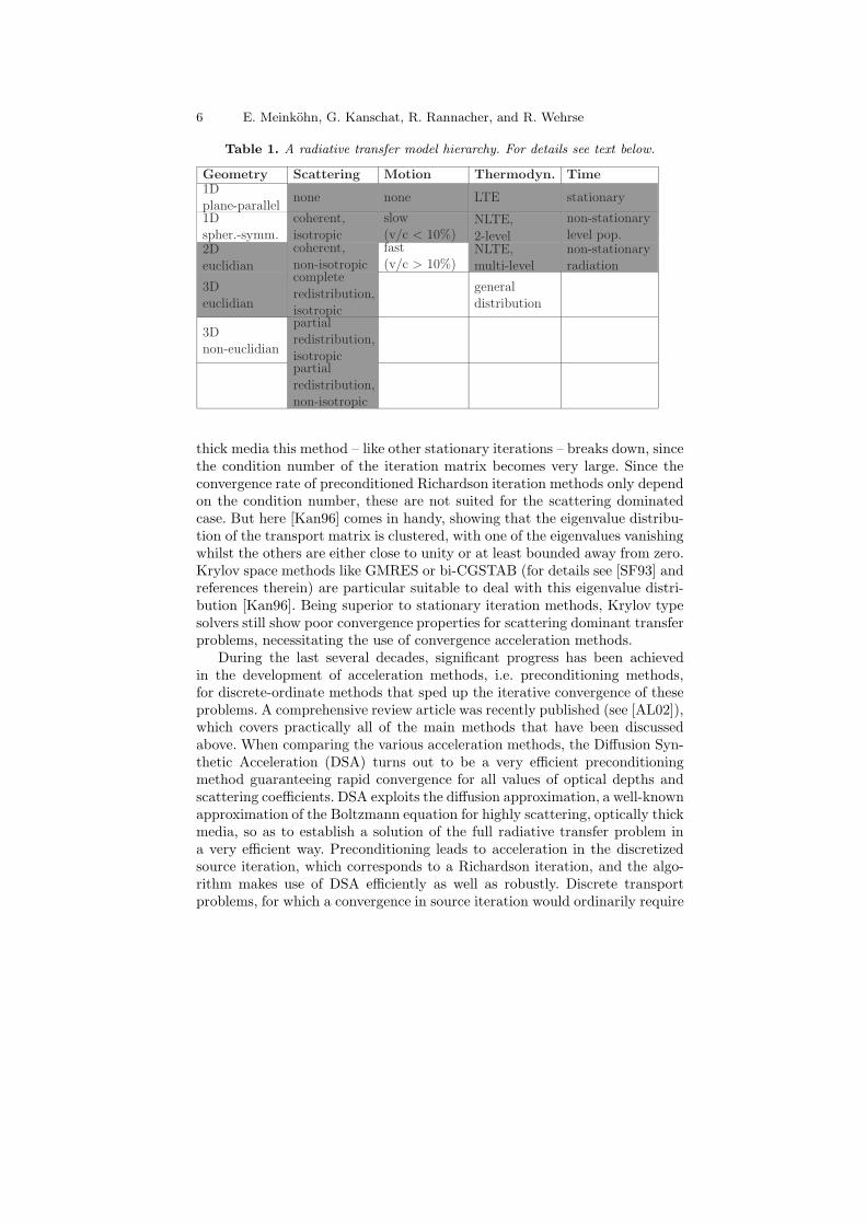
Table 1. A radiative transfer model hierarchy. For details see text below.
Geometry Scattering Motion Thermodyn. Time1Dplane-parallel
none none LTE stationary
1Dspher.-symm.
coherent,
isotropic
slow
(v/c < 10%)NLTE,
2-level
non-stationarylevel pop.
2Deuclidian
coherent,
non-isotropic
fast(v/c > 10%)
NLTE,multi-level
non-stationaryradiation
3D
euclidian
complete
redistribution,isotropic
generaldistribution
3Dnon-euclidian
partialredistribution,
isotropicpartial
redistribution,non-isotropic
thick media this method – like other stationary iterations – breaks down, sincethe condition number of the iteration matrix becomes very large. Since theconvergence rate of preconditioned Richardson iteration methods only dependon the condition number, these are not suited for the scattering dominatedcase. But here [Kan96] comes in handy, showing that the eigenvalue distribu-tion of the transport matrix is clustered, with one of the eigenvalues vanishingwhilst the others are either close to unity or at least bounded away from zero.Krylov space methods like GMRES or bi-CGSTAB (for details see [SF93] andreferences therein) are particular suitable to deal with this eigenvalue distri-bution [Kan96]. Being superior to stationary iteration methods, Krylov typesolvers still show poor convergence properties for scattering dominant transferproblems, necessitating the use of convergence acceleration methods.
During the last several decades, significant progress has been achievedin the development of acceleration methods, i.e. preconditioning methods,for discrete-ordinate methods that sped up the iterative convergence of theseproblems. A comprehensive review article was recently published (see [AL02]),which covers practically all of the main methods that have been discussedabove. When comparing the various acceleration methods, the Diffusion Syn-thetic Acceleration (DSA) turns out to be a very efficient preconditioningmethod guaranteeing rapid convergence for all values of optical depths andscattering coefficients. DSA exploits the diffusion approximation, a well-knownapproximation of the Boltzmann equation for highly scattering, optically thickmedia, so as to establish a solution of the full radiative transfer problem ina very efficient way. Preconditioning leads to acceleration in the discretizedsource iteration, which corresponds to a Richardson iteration, and the algo-rithm makes use of DSA efficiently as well as robustly. Discrete transportproblems, for which a convergence in source iteration would ordinarily require
Multidimensional radiative transfer 7
hundreds, thousands, or even millions of iteration steps, are now solved withDSA in less than a few tens iterations. Unfortunately, this method shows aloss in the effectiveness for multidimensional Cartesian grids in the presenceof material discontinuities. In [WWM04] it is shown that a Krylov iterativemethod, preconditioned with DSA, is an effective remedy that can be used toefficiently compute solutions for this class of problems. Results from numericalexperiments show that replacing source iteration with a preconditioned Krylovmethod can efficiently solve transfer problems that are virtually intractablewith accelerated source iteration (see [WWM04]).
Next to Monte-Carlo and extremely slow Angle-Moment methods (see[SL87, ER90]), only the finite difference method described in [SSW91] existedprior to the Heidelberg project of developing a robust FEM code modelingmultidimensional radiation fields in heterogeneous and highly scattering me-dia. Table 1 displays a radiative transfer model hierarchy. The marked boxescorrespond to the models the codes developed at Heidelberg University areable to deal with. The abbreviations LTE and NLTE account for local andnon-local thermodynamic equilibrium, respectively.
4 Monochromatic 3D Radiative Transfer
4.1 The Radiative Transfer Problem
Our aim is the calculation of the radiation field in diffuse matter in space.Assuming the matter is surrounded by a vacuum, we will only consider aconvex domain containing the area of interest. Radiation leaving this domainwill not enter it again. Inside this 3D domain Ω ⊂ R
3, the specific intensity Isatisfies the monochromatic radiative transfer equation
n · ∇xI(x,n) + κ(x)I(x,n)
+ σ(x)(I(x,n) − 1
4π
∫
S2
P (n′,n)I(x,n′) dω′)
= f(x),(2)
where x ∈ Ω is location in space and n is the unit vector pointing in thedirection of the solid angle dω of the unit sphere S2. The optical propertiesof the matter are given by the absorption coefficient κ(x) and the scatteringcoefficient σ(x). The angular phase function P occurring in the scatteringintegral is normalized, such that 1
4π
∫P (n′,n) dω′ = 1. The source term
f(x) = κ(x)B(T (x)) + ǫ(x) (3)
consists of thermal emission depending on a temperature distribution T (x)and an additional emissivity ǫ(x) of a point source or an extended object. Bis the Planck-Function. To be able to solve Eq. (2), boundary conditions ofthe form
I(x,n) = g(x,n) (4)
8 E. Meinkohn, G. Kanschat, R. Rannacher, and R. Wehrse
must be imposed on the “inflow boundary”
Γ− =(x,n) ∈ Γ
∣∣nΓ ·n < 0, (5)
where nΓ is the normal unit vector to the boundary surface Γ . The signof the product nΓ ·n describes the “flow direction” of the photons acrossthe boundary. If there are no light sources outside the modeled domain, thefunction g will be zero everywhere.
The left hand side of Eq. (2) will be abbreviated as an operator A appliedto the intensity function I, yielding the very compact operator form of theradiative transfer equation
AI(x,n) = f(x). (6)
As already mentioned in the introduction the resulting linear system ofalgebraic equations is usually too large and this amount of data cannot behandled even on most advanced supercomputers. The application of efficienterror estimation and grid adaption techniques is necessary to obtain reliablequantitative results. Finite element methods, in particular so-called Galerkinmethods, are most suitable for these techniques (for details see [BR01] andthe articles [BBR05, BKM05, BR05a, BR05b, CHR05] in this volume).
4.2 Finite Element Discretization
Equation (2) is analyzed in [DL00] and the natural space for finding solutionsis
W =I ∈ L2(Ω × S2)
∣∣ n · ∇xI ∈ L2(Ω × S2), (7)
where L2 is the Lebesgue space of the square integrable functions. If we con-sider homogeneous vacuum boundary condition, i.e. g(x,n) = 0, the solutionspace is
W0 =I ∈ W
∣∣ I = 0 on Γ−
. (8)
In order to apply a finite element method, we have to use a weak for-mulation of Eq. (2). Therefore, we multiply both sides of Eq. (2) by a trialfunction ϕ(x,n) and integrate over the whole domain Ω×S2. Thus, the weakformulation reads: Find I ∈ W0, such that
∫
Ω
∫
S2
n · ∇xI(x,n)ϕ(x,n) dω d3x
+
∫
Ω
∫
S2
(κ(x) + σ(x))I(x,n)ϕ(x,n) dω d3x
−∫
Ω
∫
S2
∫
S2
σ(x)P (n′,n)I(x,n′)ϕ(x,n) dω′ dω d3x
=
∫
Ω
∫
S2
f(x)ϕ(x,n) dω d3x ∀ϕ ∈ W0.
(9)
Multidimensional radiative transfer 9
By extending the definition of the L2-scalar product we introduce theabbreviation
(I, ϕ) = (I, ϕ)Ω×S2 =
∫
Ω
∫
S2
Iϕ dω d3x. (10)
Thus, the weak formulation of the operator form in Eq. (6) is
(AI, ϕ) = (f, ϕ) ∀ ϕ ∈ W0. (11)
If there is no scattering, i.e. σ(x) = 0 on Ω, the problem decouples to a systemof stationary advection equations on Ω. These equations are hyperbolic. If thesolutions are not smooth, standard finite element techniques applied to thistype of equations are known to produce spurious oscillations. We can achievestability by applying the streamline diffusion modification (see [HB82] and[Joh87]):
(AI, ϕ + δn · ∇xϕ) = (f, ϕ + δ n · ∇xϕ) ∀ ϕ ∈ W0. (12)
The cell-wise constant parameter function δ depends on the local mesh widthand the coefficients κ and σ. Note that the solution of Eq. (11) also solvesEq. (12). No additional consistency error is induced since the stabilizationterm is simply added to Eq. (11). In the following, the streamline diffusiondiscretization term will be omitted but implicitly assumed.
Applying standard Galerkin finite elements to solve Eq. (11), we choose afinite dimensional subspace Wh of W consisting of functions that are piecewisepolynomials with respect to a subdivision or triangulation Th of Ω × S2. Themesh size h is the piecewise constant function defined on each triangulationcell K by the diameter of the cell. The discrete analogon of Eq. (11) is findingIh ∈ Wh, such that
(AIh, ϕh) = (f, ϕh) ∀ ϕh ∈ Wh. (13)
The construction of the subspace Wh needs some further consideration (see[Kan96]). The discretized domain is a tensor product of two sets of completelydifferent length scales: While Ω represents a domain in geometric space, S2 isthe unit sphere in the Euclidean space R
3. Therefore, we use a tensor productsplitting of the five-dimensional domain Ω × S2, such that a grid cell of thefive-dimensional grid will be the tensor product of a two-dimensional cell Kω
and a three-dimensional cell Kx. Accordingly, the mesh sizes with respect tox and ω will be different.
On S2 we use fixed discretization based on a refined icosahedron. Quadra-ture points are the cell centers projected on S2. This projection method guar-antees equally distributed quadrature points, each associated with a solid an-gle dω of the same size. In comparison to other numerical quadrature methods,additional symmetry conditions are redundant and discretization artifacts atthe poles are avoided. Furthermore, we use piecewise constant trial functions.That way, the seven-dimensional integration of the scattering term in the
10 E. Meinkohn, G. Kanschat, R. Rannacher, and R. Wehrse
weak formulation of Eq. (9) can be calculated very efficiently. For example,the integration of the intensity over the whole unit sphere is simply replacedby a sum divided by the number of discrete ordinates M
1
4π
∫
S2
I(n) dω → 1
M
M∑
j=1
Ij . (14)
Nevertheless, our scheme is second order accurate in the evaluated ordinatepoints due to super-convergence (see [Kan96]).
For the space domain Ω we use locally refined hexahedral meshes. Themesh size of the spatial cell Kx is denoted by h. Since the boundaries arearbitrary for our astrophysical applications, we can choose a unit cube forΩ and place the simulation object within this cube. We only have ensurethat the boundary of Ω is far away from the simulation object where thephotons may freely escape towards the observer. Thus, we do not have toworry about boundary approximations. We use continuous piecewise trilineartrial functions in space.
4.3 Error Estimation and Adaptivity
The calculation of complex radiation fields in astrophysics often requires highresolution in parts of the computational domain, for example in regions withstrong opacity gradients. Then, reliable error bounds are necessary to rule outnumerical errors. Due to the high dimension of the radiative transfer problem,a well suited method for error estimation and grid adaptation is necessary toachieve results of sufficient accuracy even with the storage capacities of parallelcomputers.
In addition, computational goals in astrophysics are often more specific.The result of a simulation is to be compared with observations to developa physical model for the celestial object. For instance, in the case of a dis-tant unresolved object, the radiative energy emanating the domain Ω in one
particular direction, i.e. the direction towards the observer, is of interest.Generally, a measured quantity like the radiative energy can be expressed asa linear functional M(I). By linearity, the error of the measured quantity isM(I)−M(Ih) = M(e), where e = I − Ih. In the following, we will show thatit is possible to obtain an a-posteriori estimate for M(e), even if the exactsolution I is unknown.
Suppose, z(x,n) is the solution of the dual problem
M(ϕ) = (ϕ,A∗z) ∀ϕ ∈ W0, (15)
where the dual radiative transfer operator is defined by
A∗z(x,n) = −n · ∇xz(x,n) +(κ(x) + σ(x)
)z(x,n)
−σ(x)
∫
S2
P (n′,n)z(x,n′) dω′. (16)
Multidimensional radiative transfer 11
The boundary conditions for the dual problem are complementary to those inthe primal problem, i.e. I = 0 on the “outflow boundary” Γ+ = (x,n) ∈ Γ |nΓ ·n > 0. Then, we get the formal error representation
M(e) = (e,A∗z) = (Ae, z)
= (Ae, z − zi)
=∑
K∈Th
(f −AIh, z − zi
)K
(17)
for arbitrary zi ∈ Wh. In the second line of Eq. (17) a characteristic featureof finite element methods is used, the so-called Galerkin orthogonality
(AI −AIh, ϕh) = 0 ∀ϕh ∈ Wh. (18)
Since the dual solution z is unknown, it is a usual approach to apply Holder’sinequality and standard approximation estimates of finite element spaces 4
to obtain the duality-based a-posteriori error estimate (“DRW method”; see[BR01] and the articles [BBR05, BKM05, BR05a, BR05b, CHR05] in thisvolume)
M(e) ≤ η =∑
K∈Th
ηK , ηK = CKh2K‖‖K‖∇2z‖K , (19)
where the constant CK is determined by local approximation properties ofWh. The residual function of Ih is defined by = f −AIh. Since the dualsolution z is not available analytically, it is usually replaced by the finiteelement solution zh to the dual problem in Eq. (15). This involves a secondsolution step of the same structure as the primal problem. It is clear, that bythis replacement the error estimate in Eq. (19) is not strictly true anymore.Experience shows that the additional error is small and the estimate may beused if multiplied with a modest security factor larger than one (for detailssee [BR01]).
A first approach in the development of strategies for grid refinement basedon a-posteriori error estimates is the control of the global energy or L2-errorinvolving only local residuals of the computed solution (see [FK97]). Formally,
using the functional M(ϕ) = ‖e‖−1(e, ϕ) in Eq. (15), we obtain M(e) =
‖e‖−1(e, e) = ‖e‖ for the left hand side of (17). An estimate of the right hand
side of Eq. (17) yields
‖e‖ ≤ η =
√ ∑
K∈Th
η2L2 , ηL2 = CKCsh
2K‖‖K . (20)
In this estimate, the information about the global error sensitivities con-tained in the dual solution is condensed into just one “stability constant”
4for details see [BR01] and the standard Bramble-Hilbert theory in [BH71]
12 E. Meinkohn, G. Kanschat, R. Rannacher, and R. Wehrse
Cs =∥∥∇2z
∥∥. This is appropriate in estimating the global L2-error in case ofconstant coefficients. For more general situations with strongly varying coef-ficients, it may be advisable rather to follow the “DRW approach” in whichthe information from the dual solution is kept within the a-posteriori errorestimator defined in Eq. (19). Nevertheless, the L2-indicator ηL2 in Eq. (20)provides a reasonable grid refinement criterion to study the qualitative be-havior of the solution I everywhere in Ω (see [WMK99] for an illustration ofthis approach).
The grid refinement process on the basis of an a-posteriori error estimateis organized in the following way: Suppose that some error tolerance TOL isgiven. The aim is to find the most economical grid Th on which
|M(e)| ≤ η(Ih) =
√ ∑
K∈Th
η2K(Ih) ≤ TOL, (21)
with local refinement indicators ηK taken from Eq. (19). A qualitative investi-gation of grids obtained via different adaptive refinement criteria, e.g. Eq. (19)and Eq. (20), is published in [RM01]. Having computed the solution on acoarse grid, the so-called fixed fraction grid refinement strategy (see [Kan96],[BR01]) is applied: The cells are ordered according to the size of ηK and afixed portion ν (say 30%) of the cells with largest ηK is refined. This guaran-tees, that in each refinement cycle a sufficient large number of cells is refined.Then, a solution is computed on the new grid and the process is continued un-til the prescribed tolerance is achieved. This algorithm is especially valuable,if a computation “as accurate as possible” is desired, that is, the tolerance isnot reached, but computer memory is exhausted. Then, the parameter ν hasto be determined by the remaining memory resources.
4.4 Resulting Matrix Structure
Given a discretization with N vertices in Ω and M ordinates in S2, the discretesystem has the form
A · u = f , (22)
with the vector u containing the discrete specific intensities and the vectorf the values of the source term. Both vectors are of length (N · M). A is a(N · M) × (N · M) matrix. Applying the tensor product structure proposedabove, we may write
A = T + K + S (23)
with the block structure
Multidimensional radiative transfer 13
T =
T1 0
. . .
0 TM
, K =
K1 0
. . .
0 KM
,
S =
ω11S1 . . . ω1MS1
.... . .
...ωM1SM . . . ωMMSM
,
where ωil = P (ni,nl)/M . If we account for the finite element streamlinediffusion discretization as described in Eq. (12), the entries of the N × Nblocks are defined by
Tjki = (ϕj + δni · ∇xϕj ,ni · ∇xϕk)
Kjki = (ϕj + δni · ∇xϕj , (κ + σ)ϕk)
Sjki = (ϕj + δni · ∇xϕj , σϕk) ,
where j = 1, ..., N and k = 1, ..., N .
4.5 Iterative Methods
The linear system of equations resulting from the discretization describedabove is large (107 unknowns at least), sparse, and strongly coupled due tothe integral operator. Usually, an iterative scheme is applied to solve suchlarge systems of equations (e.g., see [Hac93, Var00]). The standard algo-rithm used in astrophysics in this case is the so-called Λ- or Source Iterationmethod [Mih78] which can be viewed as a form of the Richardson methodwith nearly block-Jacobi-preconditioning. Use of a full Jacobi preconditioneris a first step towards better convergence rates [Tur93]. Since the transportoperator is inverted explicitly, these methods converge very fast for transportdominated problems. If, further, the triangular matrix structure of upwind-discretizations is exploited, the inversion is indeed very cheap (one matrix-vector-multiplication).
Unfortunately, the present interest is in opaque and highly scattering me-dia where this method – like other stationary iterations – breaks down, becausethe condition number of the iteration matrix becomes very large. Since theconvergence rate of preconditioned Richardson iteration methods exclusivelydepends on the condition number, stationary iterations are not suited for thescattering dominated case. It can be shown, though, that the eigenvalue distri-bution of the transport matrix is clustered, with one eigenvalue located at theorigin, while the others are close to unity or at least bounded away from zero(for details see [Kan96]). Krylov space methods like GMRES or bi-CGSTABdescribed in [SF93] are particular suited to deal with such a type of eigenvaluedistribution. While Krylov-type solvers are superior to stationary iterationmethods, they still have poor convergence properties for scattering-dominated
14 E. Meinkohn, G. Kanschat, R. Rannacher, and R. Wehrse
and opaque transfer problems, so that convergence acceleration methods needto be brought in. During the last several decades, significant progress hasbeen achieved in the development of acceleration methods, i.e. precondition-ing methods, which were designed to speed up the iterative convergence ofdiscrete-ordinates approaches. A comprehensive review recently appeared inthe literature (see [AL02]), covering the main methods that have been pro-posed. Of all the acceleration methods, the Diffusion Synthetic Acceleration(DSA) is one of the most efficient preconditioning methods, guaranteeing rapidconvergence for all optical thicknesses and scattering values. In Sect. 8 a DSA-type preconditioner is presented that acts like a smoothing operator for spe-cific intensities and which corresponds to a multilevel method for the diffusionapproximation of the mean intensity. The word “multilevel” or “multigrid”often connotes a sequence of increasingly coarse spatial meshes. However, fortransport problems, space and angle are variables, and the method we considerinvolves “collapsing” the transport problem onto “coarser grids” independentof the photon direction. It is demonstrated that the method allows to arriveat a fast solution of discrete linear problems in those cases where scatteringis dominant as well as when transition regions occur.
4.6 Parallelization
Transport dominated problems differ in one specific point from elliptic prob-lems: There is a distinct direction of information flow. This has to be consid-ered in the development of parallelization strategies. While a domain decom-position for Poisson’s equation should minimize the length of interior edges,this does not yield an efficient method for transport equations.
In [Kan00], it was concluded that parallelization strategies for transportequations should not divide the domain across the transport direction. Thesolution of the radiative transfer equation consists of a number of transportinversions for different photon propagation directions. The construction of anefficient domain decomposition method would require a direction dependentsplitting of the domain Ω. Since this causes immense implementation prob-lems, we decided to use ordinate parallelization.
This strategy distributes the ordinate space S2 of the radiative transferequation. Since we use discontinuous shape functions for the ordinate variableand there is no local coupling due to the integral operator, this results in atrue non-overlapping parallelization. Clearly, it has disadvantages, too. As thescattering integral is a global operator, ordinate parallelization involves globalcommunication. In add, the resolution in space is restricted by the per nodememory and not by the total memory of the machine. In [RM01] memoryand CPU time requirements are investigated for a test model configurationdistributing the ordinate space S2 over 1 to 16 processors. The results showthat the code scales optimal (i.e. double the number of processors, halves therequired CPU time and memory) for parallel applications.

Multidimensional radiative transfer 15
5 Polychromatic 3D Line Transfer
In the following an algorithm modeling polychromatic, i.e. frequency-depen-dent, 3D radiation fields in moving media is presented. This extension of themonochromatic model described in the previous section is required, since theradiation field is of major importance for the energy transfer in many differ-entially moving celestial objects like novae, supernovae, collapsing molecularclouds, collapsing and expanding or rotating gas clouds (halos), and accretiondiscs. Additionally, resonance line profiles are strongly affected by radiativetransfer processes, providing deep insight into the density structure and thenature of the macroscopic velocity field of the emanating object.
The present work aims at the modeling of 3D radiation fields in gas cloudsfrom the early universe, in particular as to the influence of varying distri-butions of density and velocity. In observations of high-redshift gas clouds(halos), the Lyα transition from the first excited energy level to the groundstate of the hydrogen atom is usually found to be the only prominent emissionline in the entire spectrum. It is a well-known assumption that high-redshiftedhydrogen clouds are the precursors of present-day galaxies. Thus, the inves-tigation of the Lyα line is of paramount importance for the theory of galaxyformation and evolution. The observed Lyα line – or rather, to be precise,its profile – reveals both the complexity of the spatial distribution and of thekinematics of the interstellar gas, and also the nature of the photon source.
The transfer of resonance line photons is profoundly determined by scatter-ing in space and frequency. Analytical (see [Neu90]) as well as early numericalmethods [Ada72, HK80] were restricted to one-dimensional, static media. Onlyrecently, codes based on the Monte Carlo method were developed which arecapable to investigate the more general case of a multi-dimensional medium(see [ALL01, ALL02, ZM02]).
5.1 Line Transfer in Moving Media
The frequency-dependent radiation field in moving media is obtained by solv-ing the non-relativistic radiative transfer equation in a co-moving frame (fordetails see [WBW00]). For a three-dimensional domain Ω the operator formof the equation is
(T + D + S + χ(x, ν)
)I(x,n, ν) = f(x, ν). (24)
T is the transfer operator, D the “Doppler” operator, and S the scatteringoperator, which are defined as follows
T I(x,n, ν) = n · ∇xI(x,n, ν),
DI(x,n, ν) = w(x,n) ν∂
∂νI(x,n, ν),
SI(x,n, ν) = −σ(x)
4π
∫ ∞
0
∫
S2
R(n, ν;n, ν)I(x, n, ν) dω dν.
16 E. Meinkohn, G. Kanschat, R. Rannacher, and R. Wehrse
The relativistic invariant specific intensity I is a function of six variables, threeof which give the spatial location x, while two variables give the direction n
(pointing in the direction of the solid angle dω of the unit sphere S2), andone variable gives the frequency ν.
The extinction coefficient χ(x, ν) = κ(x, ν) + σ(x, ν) is the sum ofthe absorption coefficient κ(x, ν) = κ(x)ϕ(ν) and the scattering coefficientσ(x, ν) = σ(x)ϕ(ν). The frequency-dependence is given by a normalized pro-file function ϕ ∈ L1(R+). The core of the Lyα line is dominated by Dopplerbroadening. The effects of radiation and resonance damping may be impor-tant in the wings of the line at low column densities. Under the assumptionthat these mechanisms are all uncorrelated, one can account for their com-bined effects by a convolution procedure. The folding of the Doppler profilewith the Lorentz profiles from radiation and resonance damping gives a Voigtprofile, which is the general description of Lyα line profiles (see [Mih78]). Forall applications presented in this paper vturb ≫ vtherm is adopted. This resultsin a very broad Doppler core dominating the Lorentzian wings of the Voigtprofile. Thus, a Doppler profile
ϕ(ν) =1√
π ∆νD
exp
[−(
ν − ν0
∆νD
)2]
(25)
is a reasonable description of a Lyα line profile, where ν0 is the frequency ofthe line center and c is the speed of light. The Doppler width ∆νD and theDoppler velocity vD are determined by a thermal velocity vtherm and a smallscale turbulent velocity vturb,
∆νD =ν0
cvD =
ν0
c
√v2therm
+ v2turb
. (26)
For the source term
f(x, ν) = κ(x, ν)B(T (x), ν) + ǫ(x, ν), (27)
we can consider thermal radiation and non-thermal radiation. In the case ofthermal radiation, f is calculated from a temperature distribution T (x), whereB(T, ν) is the Planck function.
The “Doppler” operator D causes the Doppler shift of the photons. Aderivation for non-relativistic moving media 5 can be found in [WBW00]. Thebasis of the derivation is a “simplified” Lorentz transformation, which, in fact,is a Galilei transformation in combination with a linear Doppler formula. Werestrict ourselves to sufficiently small velocity fields, and furthermore neglectaberration and advection effects, i.e. the photon propagation direction n iskept unchanged during the transformation. The function
w(x,n) = −n · ∇x
(n · v(x)
c
)(28)
5This includes velocities fields up to approximately 10% of the speed of light
Multidimensional radiative transfer 17
is the gradient of the velocity field v(x) in direction n. Note that the sign ofw may change depending on the complexity of the velocity field v.
Line transfer problems often include scattering processes where both thedirection and the frequency of a photon may be changed. These changes aredescribed by a general redistribution function R(n, ν;n, ν) which gives thejoint probability that a photon will be scattered from direction n in solidangle dω and frequency range (ν, ν + dν) into solid angle dω in direction n
and frequency range (ν, ν +dν). If we assume that the radiation field is nearlyisotropic, the scattering process may be approximated by
SI = −σ(x)
4π
∞∫
0
R(ν, ν)
∫
S2
I(x, n, ν) dω dν, (29)
where R(ν, ν) is the angle-averaged redistribution function
R(ν, ν) =1
(4π)2
∫
S2
∫
S2
R(x, n, ν;n, ν) dω dω. (30)
The function defined by Eq. (30) is normalized such that
∞∫
0
∞∫
0
R(ν, ν) dν dν = 1. (31)
For the calculations in Sect. 5.3, we consider two limiting cases: strict coher-ence and complete redistribution in the comoving frame. In the former case,we have
R(ν, ν) = ϕ(ν)δ(ν − ν), (32)
and in the latterR(ν, ν) = ϕ(ν)ϕ(ν). (33)
Thus, for coherent isotropic scattering, the scattering term simplifies to
ScohI(x,n, ν) = −σ(x, ν)
4π
∫
S2
I(x, n, ν) dω (34)
In the case of complete redistribution, the photons are scattered isotropicallyin angle, but are randomly redistributed over the line profile. Then, the scat-tering term reads
ScrdI(x,n, ν) = −σ(x, ν)
4π
∫ ∞
0
ϕ(ν)
∫
S2
I(x, n, ν) dω dν. (35)
5.2 Boundary Conditions
Formally, the frequency derivative in the Doppler term of (24) can be viewedas being similar to the time derivative for non-stationary radiative transfer or
18 E. Meinkohn, G. Kanschat, R. Rannacher, and R. Wehrse
heat transfer problems, so that a parabolic system of initial value problems isobtained. Unfortunately, the Doppler term also contains a function w(x,n),which is essentially the gradient of the macroscopic velocity field, multiplied bythe photon propagation direction n (cf. (28)). Depending on the complexity ofthe velocity field, this function w(x,n) may change its sign at different pointsx and for different directions n when setting up the initial value either on thelower or upper frequency boundary. In this paper we take this into accountby defining an additional frequency boundary value problem, which involvesa “frequency inflow boundary” Σ− = Ω × S2 × ∂Λ depending on the sign ofw(x,n). In order to solve (24) correctly, boundary conditions of the form
I(x,n, ν) = p(x,n, ν) on Γ− × Λ and (36)
I(x,n, ν) = q(x,n, ν) on Σ−. (37)
must be imposed. The “spatial inflow boundary” is
Γ− × Λ =(x,n, ν) ∈ Γ
∣∣∣ nΓ · n < 0, (38)
where nΓ is the normal unit vector to the boundary surface Γ of the spatialdomain Ω. The sign of the product nΓ ·n describes the “flow direction” of thephotons across the boundary of the spatial domain. For our modeling of thespectral Lyα line, we assume that there is no continuum emission “outside ofthe line” and that there are no light sources “outside the modeled domain”. Inthis case the two boundary conditions for the solution of the transfer equation(24) in moving media are
I(x,n, ν) = 0 on Σ−, (39)
I(x,n, ν) = 0 on Γ− × Λ. (40)
5.3 Finite Element Discretization
The simultaneous Galerkin discretization in space-frequency is, from a the-oretical point of view, an extremely appealing approach. Considering thememory requirement, the solution of the complete algebraic system result-ing from this discretization is by far too “expensive”. With a view to reducingthe memory demand, a discretization first in space and then in frequencyis performed. This approach is called method of lines and finally resultsin a system of ordinary differential equations. Contrary to the continuousGalerkin discretization in space, the discretization in frequency is a discontin-uous Galerkin (DG) method. It is important to note that the above discretiza-tion in space and in frequency can be interpreted as a simultaneous Galerkindiscretization in the space-frequency domain. The frequency DG method isperformed by using piecewise polynomials of degree zero, which correspondsto an implicit Euler method for N equidistantly distributed frequency pointsνi ∈
ν1, ν2, ..., νN
⊂ Λ (see [Boe96]). DG methods are not only used for
Multidimensional radiative transfer 19
discretizing ordinary differential equations, especially initial value problems,but also for the time discretization and mesh control of partial differentialequations as described in [EJ87, EJ91] and [EJT85].
Discretization for Coherent Scattering
In order to solve the radiative transfer equation (24), we first carry out thefrequency discretization including coherent scattering. With the abbreviation
Acoh = T + Scoh + χ(x, ν) (41)
Eq. (24) can be written as
AcohI(x,n, ν) + w(x,n)ν∂
∂νI(x,n, ν) = f(x, ν). (42)
Since the function w(x,n) may change its sign, this simple difference schemefor the Doppler term reads
w(x,n)ν∂I∂ν
−→ wνi
Ii − Ii−1
∆ν(wi > 0), (43)
and
w(x,n)ν∂I∂ν
−→ wνi
Ii+1 − Ii
∆ν(wi < 0), (44)
where ∆ν is the constant frequency step size. All quantities referring to thediscrete frequency point νi are denoted by an index “i”. Employing the Eulermethod, we get a semi-discrete representation of Eq. (42)
(Acoh
i +|w|νi
∆ν
)Ii = fi +
|w|νi
∆ν
Ii−1 (w > 0)Ii+1 (w < 0)
. (45)
The additional term on the left side of Eq. (45) can be interpreted as an ar-tificial opacity, which is advantageous for the solution of the resulting linearsystem of equations. The additional term on the right side of Eq. (45) is in-cluded as an artificial source term. Equation (45) can be written in a compactoperator form
Acohi Ii = fi. (46)
Given a discretization with L degrees of freedom in Ω, M directions on theunit sphere S2 and N frequency points, the overall discrete system has thematrix form
Acohu = f , (47)
with the vector u containing the discrete intensities and the vector f thevalues of the source term for all frequency points νi. Both vectors are oflength (L · M · N) and Acoh is a (L · M · N) × (L · M · N) matrix. The fact
20 E. Meinkohn, G. Kanschat, R. Rannacher, and R. Wehrse
that the function w(x,n) may change its sign, results in a block-tridiagonalstructure of Acoh and we get
Acoh1 R1 0 . . . 0
B2 Acoh2 R2
. . ....
0. . .
. . .. . . 0
.... . .
. . .. . . RN−1
0 . . . 0 BN AcohN
u1
u2
...
...uN
=
f1f2......
fN
. (48)
According to the sign of w(x,n) the block matrices Ri and Bi hold entries ofw(x,n)νi/∆ν causing a redshift and blueshift of the photons in the medium,respectively. Requiring a reasonable resolution, the resulting linear system ofequations of the total system is too large to be solved directly. Hence, we aretreating N “monochromatic” radiative transfer problems
Acohi ui = fi, (49)
with a slightly modified right hand side
fi = fi + Riui+1 + Biui−1. (50)
Note that using simple velocity fields (e.g. collapse or expansion of a gascloud) the sign of w(x,n) is fixed and the matrix Acoh has a block-bidiagonalstructure. This is favorable for our solution strategy, since we only need tosolve Eq. (49) once for each frequency point.
Discretization for Complete Redistribution
In order to include complete redistribution, we use a simple quadraturemethod for the frequency integral in the scattering operator Scrd in Eq. (35).The Doppler term is discretized using an implicit Euler scheme as describedin the previous section. Starting from N equidistantly distributed frequencypoints νi ∈
ν1, ν2, ..., νN
⊂ Λ and N weights q1, q2, ..., qN , we define a
quadrature method
Q(νi) :=N∑
j=1
qjξ(νj) (51)
for integrals∫
Λξ(ν′)dν′. In the case of complete redistribution the kernel is
ξ(νj) =ϕ(νj)
4π
∫
S2
I(x, n, νj)dω, (52)
and the semi-discretized scattering integral in Eq. (35) for a particular fre-quency point ∋i reads
Multidimensional radiative transfer 21
σi
4πϕiqi
∫
S2
Iidω +σi
4π
N∑
j 6=i
ϕjqj
∫
S2
I(x, n, νj)dω. (53)
With this scattering operator the semi-discrete formulation of the transferproblem for each frequency point ∋i is
(Acrd
i +|w|νi
∆ν
)Ii = fi +
σi
4π
N∑
j 6=i
ϕjqj
∫
S2
I(x, n, νj)dω, (54)
whereAcrd
i = T + χi + ϕiqiScoh. (55)
The additional terms on the right hand side of Eq. (54) must be interpretedas artificial source terms. Eq. (54) can also be written in a compact operatorform
Acrdi Ii = fi. (56)
The total discrete system has the matrix form (cf. Eq. (47))
Acrdu = f . (57)
Unfortunately, the global frequency coupling via the scattering integral inEq. (35) results in a full block matrix and we get
Acrd =
Acrd1 R1 + Q2 Q3 . . . QN
B2 + Q1 Acrd2 R2 + Q3
. . ....
Q1
. . .. . .
. . ....
.... . .
. . .. . .
...
Q1 . . . . . . . . . AcrdN
. (58)
Bi and Ri again contain the contribution of the Doppler factor w(x,n)νi/∆ν,whereas Qj holds the terms from the quadrature scheme. As we already ex-plained in the case of coherent scattering, we do not directly solve the totalsystem, but successively solve N “monochromatic” radiative transfer prob-lems
Acrdi ui = fi, (59)
successively, with a modified right hand side
fi = fi + Riui+1 + Biui−1 +∑
j 6=i
Qjuj . (60)
22 E. Meinkohn, G. Kanschat, R. Rannacher, and R. Wehrse
5.4 Full Solution Algorithm
Equation (46) and (56) are of the same form as the monochromatic radiativetransfer equation, cf. Eq. (6), for which we propose a solution method basedon a finite element technique in Sect. 4. The finite element method employshierarchically structured grids which are locally refined by means of duality-based a-posteriori error estimates. Now, we apply this method to Eq. (46) orEq. (56). The solution is obtained using an iterative procedure, where quasi-monochromatic radiative transfer problems are solved successively. In brief,the full solution algorithm reads:
1. Start with I = 0 for all frequencies.2. Solve Eq. (47) or Eq. (57) for i = 1, .., N .3. Repeat step 2 until convergence is reached.4. Refine grid and repeat steps 2 and 3.
We start with a relatively coarse grid, where only the most important struc-tures are pre-refined, and assure that the frequency interval [ν1, νN ] is wideenough to cover the total line profile. Then, we solve Eq. (46) or Eq. (56)for each frequency several times depending on the choice of the redistributionfunction and the velocity field. During this fixed point iteration, we mon-itor the changes of the resulting line profile in a particular direction nout.When the line profile remains unchanged, we turn to step 4 and refine thespatial grid. Again, we apply the fixed fraction grid refinement strategy:The cells are ordered according to the size of the local refinement indica-tor ηK = max(ηK(νi))|νi
and a fixed portion of the cells with largest ηK isrefined. ηK(νi) is an indicator for the error contribution of the solution in cellK at frequency νi.
6 Test Calculations
The simple 3D test calculations presented in this section use a sphericallysymmetric density distribution of the form
χ(x) =
χ0/(1 + αr2c ) for r ≤ rc,
χ0/(1 + αr2) for rc < r ≤ rh,χ0/(1 + αr2
h)/103 for r > rh,(61)
where rc is a constant core radius in the center of the halo. The halo radiusis rh and the square of the radius is r2 = x2 + y2 + z2. The constant opacityχ0 is determined by the line center optical depth
τ =
∫ rh
rc
χ(x)ϕ(ν0) nthick dx (62)
between rc and rh along the most optical thick photon direction nthick. Intotal, the spatial distribution of χ is determined by three parameters: the
Multidimensional radiative transfer 23
radii rc and rh, the dimensionless parameter α, and the optical depth τ . Forrc, rh and α we use the values given in Table 2.
Since we are predominantly interested in the transfer of radiation in reso-nance lines like Lyα, we assume σ(x) = χ(x) and κ(x) = 0 for all calculationspresented here. This restricts us to the use of a given source function. In par-ticular, we consider a single spatially confined source region located at theorigin of the unit cube at the position xi = 0 with radius rs:
f(x, ν) =
ϕ(ν) for |x − xi| ≤ rs
0 for |x − xi| > rs. (63)
The function ϕ(ν) is the Doppler profile defined in Eq. (25).In general, the finite element code is able to consider arbitrary velocity
fields. For velocity fields defined on a discrete grid, e.g. resulting from hydro-dynamical simulations, the velocity gradient in direction n must be obtainednumerically. Here, we use two simple velocity fields and calculate the functionw analytically.
The first velocity field describes a spherically symmetric collapsing (v0 < 0)or expanding (v0 > 0) medium and is of the form
vio = v0
(r0
r
)l x
r, (64)
where r = |x| and v0 the scalar velocity at radius r0. The corresponding wfunction is
w(x,n) = v0
(r0
r
)l(
1
r− (l + 1)
|nx|r3
). (65)
For the second velocity field, we assume rotation around the z-axis
vrot = v0
(R0
R
)l
R−1
y
−x0
, (66)
where R2 = x2 + y2 is the distance from the rotational axis and v0 the scalarvelocity at distance R0. For n = (nx, ny, nz), the w function reads
w = v0
(R0
R
)l
(l + 1)
(xy(n2
y − n2x) + nxny(x2 − y2)
R3
). (67)
Fig. 1 shows the results of the finite element code for different optical depths,velocity fields and redistribution functions. We used 41 frequencies equallyspaced in the interval (ν − ν0)/∆νD = [−4, 6] and 80 directions. Startingwith a grid of 43 cells and a pre-refined source region, we needed 3–5 spatialrefinement steps.
For the simplest case of a static model configuration with coherent isotropicscattering even analytical solutions exist (see [RM01]). Fig. 1a displays the
24 E. Meinkohn, G. Kanschat, R. Rannacher, and R. Wehrse
Table 2. Parameters used for all calculations. Distances are given in units of thecomputational unit cube.
rh rc α rs vD v0 r0 R0
1.0 0.2 103 0.2 10−3c −10−3c 0.2 1.0
a)
−4 −2 0 2 4 6(ν−ν0)/νD
0.00
0.02
Fν
0.1110100
−0.5 0.0 0.5
0.030
0.032
0.034
b)
−6 −4 −2 0 2 4 6(ν−ν0)/νD
0.00
0.02
Fν
00.52
c)
−6 −4 −2 0 2 4 6(ν−ν0)/νD
0.00
0.02
Fν
0.1110100
d)
−6 −4 −2 0 2 4 6(ν−ν0)/νD
0.00
0.02
Fν
00.52
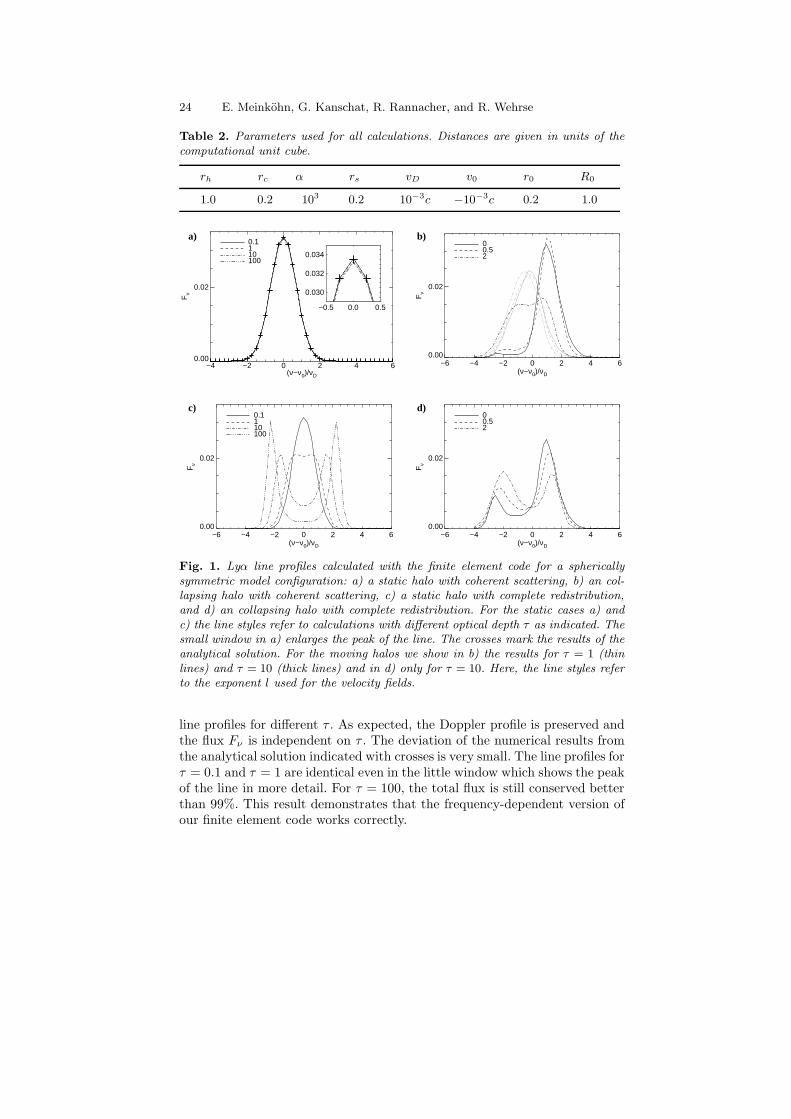
Fig. 1. Lyα line profiles calculated with the finite element code for a sphericallysymmetric model configuration: a) a static halo with coherent scattering, b) an col-lapsing halo with coherent scattering, c) a static halo with complete redistribution,and d) an collapsing halo with complete redistribution. For the static cases a) andc) the line styles refer to calculations with different optical depth τ as indicated. Thesmall window in a) enlarges the peak of the line. The crosses mark the results of theanalytical solution. For the moving halos we show in b) the results for τ = 1 (thinlines) and τ = 10 (thick lines) and in d) only for τ = 10. Here, the line styles referto the exponent l used for the velocity fields.
line profiles for different τ . As expected, the Doppler profile is preserved andthe flux Fν is independent on τ . The deviation of the numerical results fromthe analytical solution indicated with crosses is very small. The line profiles forτ = 0.1 and τ = 1 are identical even in the little window which shows the peakof the line in more detail. For τ = 100, the total flux is still conserved betterthan 99%. This result demonstrates that the frequency-dependent version ofour finite element code works correctly.
Multidimensional radiative transfer 25
Next, we consider a collapsing halo with coherent scattering and show theeffects of frequency coupling due to the Doppler term. The line profiles inFig. 1b are plotted for different exponents l of the velocity field vio definedin Eq. (64). The line profiles are redshifted for τ = 1 (thin lines). Most of thephotons directly travel through the part of the halo moving away from theobserver. Since the Doppler term is proportional to the gradient of the velocityfield, the redshift is larger for a greater exponent l. For τ = 10 (thick lines),the line profiles are blueshifted. Before photons escape from the optically thickpart of the halo in front of the source, they are back-scattered and blueshiftedin the approaching part of the halo behind the source. The blueshift is lesspronounced for the accelerated inflow with l = 2, because the strong gradientof the velocity field leads to a slight redshift in the very inner parts of thehalo. In this region, the total optical depth is still small. Further out, wherethe total optical depth increases, the line profile becomes blueshifted.
Complete redistribution leads to an even stronger coupling than theDoppler effect (see Sect. 3). The line profiles obtained for a static model withcomplete redistribution are displayed in Fig. 1c for different τ . With increas-ing optical depth the photons more and more escape through the line wings.For τ ≥ 1, we get a double-peaked line profile with an absorption trough inthe line center. The greater τ the larger the distance between the peaks andthe depth of the absorption trough. Since our frequency resolution is too poorfor the narrow wings, the flux conservation is only 96% for τ = 100.
Fig. 1d shows the results for an collapsing halo with complete redistribu-tion for τ = 10 and different exponents l. For l = 0 and l = 0.5 the collapsingmotion of the halo enhances the blue wing of the double-peaked line profile.Equally, an expanding halo would enhance the red peak. But for l = 2, thered peak is slightly enhanced for an collapsing halo due to the strong ve-locity gradient, as explained above. This example allows an insight into themechanisms of resonance line formation and shows the necessity of a profoundmultidimensional treatment.
7 Applications
All calculations discussed in this section were performed with complete re-distribution. We used 49 equidistant frequencies covering the interval (ν −ν0)/∆νD = [−6, 6], 80 directions and started from a grid with 43 cells andpre-refined source regions, which results in several 103 cells for the initialmesh. 3–7 refinement steps were performed leading to approximately 105 cellsfor the finest grid.
7.1 Elliptical Halos
As a first step towards a full three-dimensional problem without any symme-tries, we investigated an axially symmetric, disk-like model configuration with
26 E. Meinkohn, G. Kanschat, R. Rannacher, and R. Wehrse
a) b)
0.000
0.005
0.010
0.01590o
70o
55o
20o
-6 -4 -2 0 2 4 60.000
0.005
0.010
0.01590o
70o
55o
20o
0.000
0.005
0.010
0.01590o
70o
55o
20o
=1
=10
=100
F
F
F
-6 -4 -2 0 2 4 6( 0)=D
90 20-1.0
-0.5
0.0
0.5
1.0
-1.0
-0.5
0.0
0.5
1.0
-1.0
-0.5
0.0
0.5
1.0
-1.0
-0.5
0.0
0.5
1.0
-1.0
-0.5
0.0
0.5
1.0
-1.0
-0.5
0.0
0.5
1.0
1.0
0.5
0.0
-0.5
-1.0
s =1
1.0
0.5
0.0
-0.5
-1.0
s =10
1.0
0.5
0.0
-0.5
-1.0
s =100
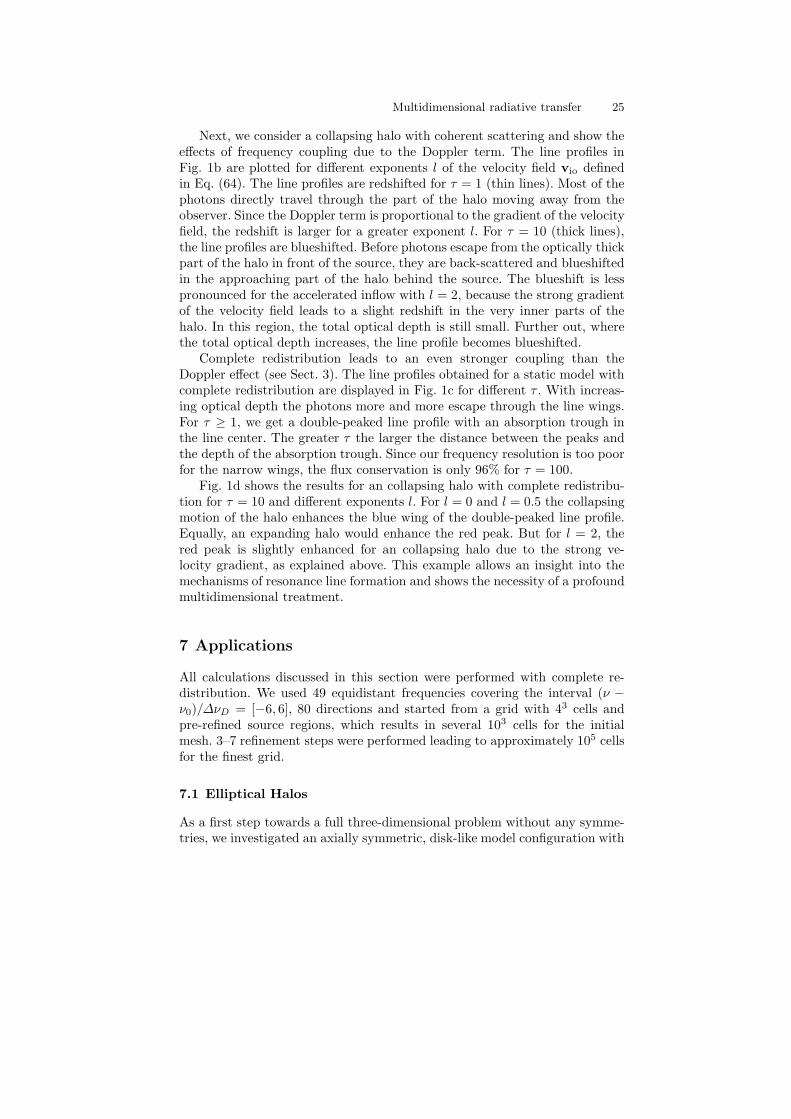
-6 -4 -2 0 2 4( 0)=D -6 -4 -2 0 2 4 6( 0)=DFig. 2. Results obtained for a disk-like model configuration with global inflow mo-tion (l = 0.5): a) Line profiles for different viewing angles and optical depthsτ = τ (nthick). b) Two-dimensional spectra for an edge-on view (90) and a nearlyface-on view (20) and different optical depths. The parameter s gives the spatialposition within a slit covering the “visible” part of the disk-like halo. The contoursare given for 2.5%, 5%, 7.5%, 10%, 20%, ..., 90% of the maximum value.
r2 = (x/3)2+(y/3)2+z2 in Eq. (61), and with a single source located at x = 0for several τ = τ(nthick) and for different velocity fields. The most opticallythick direction nthick is the direction within the equatorial plane of the disk.The direction perpendicular to the equatorial plane is the z-axis which wealso call rotational axis even for cases without rotation.
First, we consider an inflow velocity field with l = 0.5 suitable for a gravi-tational collapse. Fig. 2a displays the calculated line profiles for different τ andviewing angles. As expected, the blue peak of the line is enhanced. The higherτ the stronger the blue peak. Two-dimensional spectra from high-resolutionspectroscopy provide frequency-dependent data for only one spatial direction.This is achieved using so-called slit masks for telescope observations. In orderto compare our results with these observations we calculated two-dimensionalspectra in Fig. 2b using the data within a slit covering the “visible” partof the disk-like halo, i.e. the observable spatial distribution of the frequencyintegrated intensity. For low optical depth, the shape of the contour lines isa triangle. Photons changing frequency in order to escape via the blue wing
Multidimensional radiative transfer 27
a) b)
0.000
0.005
0.010
0.01590o
70o
55o
20o
-6 -4 -2 0 2 4 60.000
0.005
0.010
0.01590o
70o
55o
20o
=1
=10
F
F
-6 -4 -2 0 2 4 6( 0)=D
90 20-1.0
-0.5
0.0
0.5
1.0
-1.0
-0.5
0.0
0.5
1.0
-1.0
-0.5
0.0
0.5
1.0
-1.0
-0.5
0.0
0.5
1.0
1.0
0.5
0.0
-0.5
-1.0
s =1
1.0
0.5
0.0
-0.5
-1.0
s =10
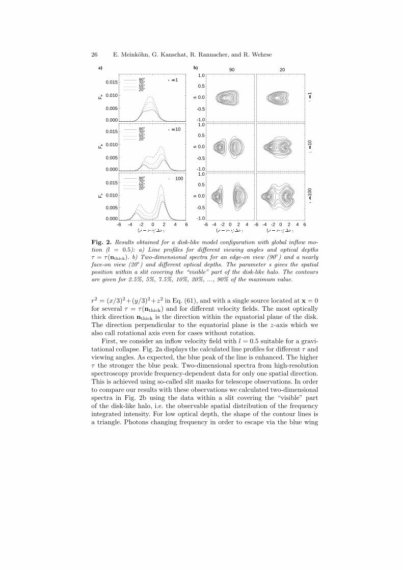
-6 -4 -2 0 2 4( 0)=D -6 -4 -2 0 2 4 6( 0)=DFig. 3. Results obtained for a disk-like model configuration with Keplerian rotation(l = 0.5) around the z-axis: a) Line profiles for different viewing angles and opticaldepths τ = τ (nthick). b) Two-dimensional spectra for an edge-on view (90) and anearly face-on view (20) and different optical depths. The parameter s gives thespatial position within a slit covering the “visible” part of the disk-like halo. Thecontours are given for 2.5%, 5%, 7.5%, 10%, 20%, ..., 90% of the maximum value.
are also scattered in space. The consequence is the greater spatial extent ofthe blue wing. Apart from a growing gap between the two peaks with higheroptical depth, the general triangular shape in conserved.
Next, we investigated the disk-like model configuration with Keplerianrotation (l = 0.5), where the z-axis is the axis of rotation. The results areplotted in Fig. 3 for τ = 1 and τ = 10. The calculated line profiles appearto be symmetric with respect to the line center and show the same behaviorwith increasing optical depths as in the static case. However, the extensionof the line wings towards higher and lower frequencies is strongly increasingwith increasing viewing angle because of the growing effect of the velocityfield. Rotation is clearly visible in the two-dimensional spectra (Fig. 3b). Theshear of the contour lines is the characteristical pattern indicating rotationalmotion. For an edge-on view at τ = 10, Keplerian rotation produces twobanana-shaped emission regions.
Finally, Fig. 7.1 depicts the spatial intensity distribution for particularfrequency points within the interval (ν − ν0)/∆νD = [−2, +2] (rows) and fordifferent viewing angles (columns). The left figure shows the results obtainedfor a disk-like model configuration with global inflow motion (l = 0.5). Theright figure shows the results obtained for a disk-like model configuration withKeplerian rotation (l = 0.5) around the z-axis. The intensity increases fromblue to white.
28 E. Meinkohn, G. Kanschat, R. Rannacher, and R. Wehrse
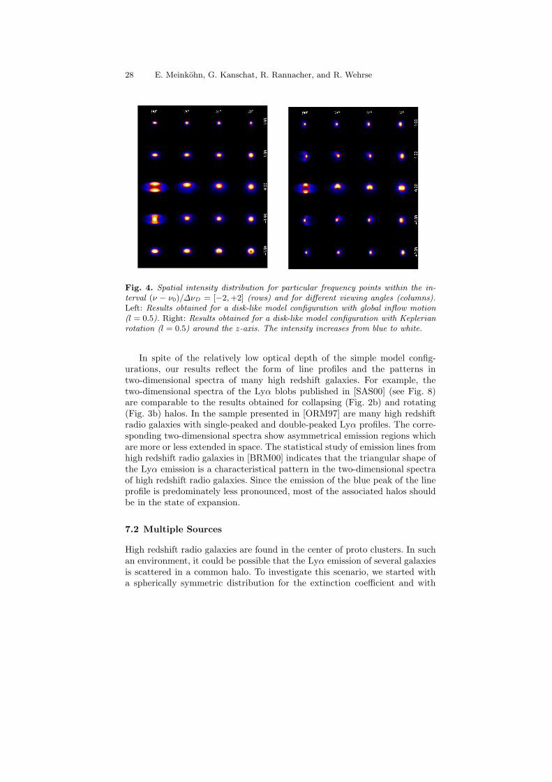
Fig. 4. Spatial intensity distribution for particular frequency points within the in-terval (ν − ν0)/∆νD = [−2, +2] (rows) and for different viewing angles (columns).Left: Results obtained for a disk-like model configuration with global inflow motion(l = 0.5). Right: Results obtained for a disk-like model configuration with Keplerianrotation (l = 0.5) around the z-axis. The intensity increases from blue to white.
In spite of the relatively low optical depth of the simple model config-urations, our results reflect the form of line profiles and the patterns intwo-dimensional spectra of many high redshift galaxies. For example, thetwo-dimensional spectra of the Lyα blobs published in [SAS00] (see Fig. 8)are comparable to the results obtained for collapsing (Fig. 2b) and rotating(Fig. 3b) halos. In the sample presented in [ORM97] are many high redshiftradio galaxies with single-peaked and double-peaked Lyα profiles. The corre-sponding two-dimensional spectra show asymmetrical emission regions whichare more or less extended in space. The statistical study of emission lines fromhigh redshift radio galaxies in [BRM00] indicates that the triangular shape ofthe Lyα emission is a characteristical pattern in the two-dimensional spectraof high redshift radio galaxies. Since the emission of the blue peak of the lineprofile is predominately less pronounced, most of the associated halos shouldbe in the state of expansion.
7.2 Multiple Sources
High redshift radio galaxies are found in the center of proto clusters. In suchan environment, it could be possible that the Lyα emission of several galaxiesis scattered in a common halo. To investigate this scenario, we started witha spherically symmetric distribution for the extinction coefficient and with
Multidimensional radiative transfer 29
a)
-1.0
-0.5
0.0
0.5
1.0
-1.0
-0.5
0.0
0.5
1.0
-1.0
-0.5
0.0
0.5
1.0
-1.0
-0.5
0.0
0.5
1.01.0
0.5
0.0
-0.5
-1.0-1.0 -0.5 0.0 0.5
s-1.0 -0.5 0.0 0.5
s-1.0 -0.5 0.0 0.5
s-1.0 -0.5 0.0 0.5 1.0
s
70Æ
Æ
50Æ
Æ
35Æ
Æ
10Æ
Æ
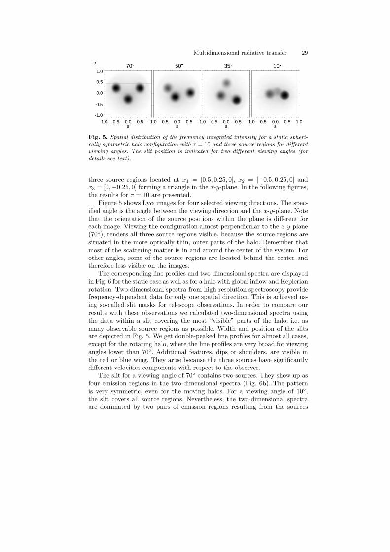
Fig. 5. Spatial distribution of the frequency integrated intensity for a static spheri-cally symmetric halo configuration with τ = 10 and three source regions for differentviewing angles. The slit position is indicated for two different viewing angles (fordetails see text).
three source regions located at x1 = [0.5, 0.25, 0], x2 = [−0.5, 0.25, 0] andx3 = [0,−0.25, 0] forming a triangle in the x-y-plane. In the following figures,the results for τ = 10 are presented.
Figure 5 shows Lyα images for four selected viewing directions. The spec-ified angle is the angle between the viewing direction and the x-y-plane. Notethat the orientation of the source positions within the plane is different foreach image. Viewing the configuration almost perpendicular to the x-y-plane(70), renders all three source regions visible, because the source regions aresituated in the more optically thin, outer parts of the halo. Remember thatmost of the scattering matter is in and around the center of the system. Forother angles, some of the source regions are located behind the center andtherefore less visible on the images.
The corresponding line profiles and two-dimensional spectra are displayedin Fig. 6 for the static case as well as for a halo with global inflow and Keplerianrotation. Two-dimensional spectra from high-resolution spectroscopy providefrequency-dependent data for only one spatial direction. This is achieved us-ing so-called slit masks for telescope observations. In order to compare ourresults with these observations we calculated two-dimensional spectra usingthe data within a slit covering the most “visible” parts of the halo, i.e. asmany observable source regions as possible. Width and position of the slitsare depicted in Fig. 5. We get double-peaked line profiles for almost all cases,except for the rotating halo, where the line profiles are very broad for viewingangles lower than 70. Additional features, dips or shoulders, are visible inthe red or blue wing. They arise because the three sources have significantlydifferent velocities components with respect to the observer.
The slit for a viewing angle of 70 contains two sources. They show up asfour emission regions in the two-dimensional spectra (Fig. 6b). The patternis very symmetric, even for the moving halos. For a viewing angle of 10,the slit covers all source regions. Nevertheless, the two-dimensional spectraare dominated by two pairs of emission regions resulting from the sources
30 E. Meinkohn, G. Kanschat, R. Rannacher, and R. Wehrse
a) b)
0.00
0.02
0.04
0.06
0.08
F
-6 -4 -2 0 2 4 60.00
0.02
0.04
0.06
0.08
F
70o
50o
35o
10o
0.00
0.02
0.04
0.06
0.08
F
70o
50o
35o
10o
static
inflow
rotation
F
F
F
-6 -4 -2 0 2 4 6( 0)=D
70Æ 10Æ-1.0
-0.5
0.0
0.5
1.0
-1.0
-0.5
0.0
0.5
1.0
-1.0
-0.5
0.0
0.5
1.0
-1.0
-0.5
0.0
0.5
1.0
-1.0
-0.5
0.0
0.5
1.0
-1.0
-0.5
0.0
0.5
1.0
1.0
0.5
0.0
-0.5
-1.0
s
stat
ic
1.0
0.5
0.0
-0.5
-1.0
s
inflo
w
1.0
0.5
0.0
-0.5
-1.0
s
rota
tion
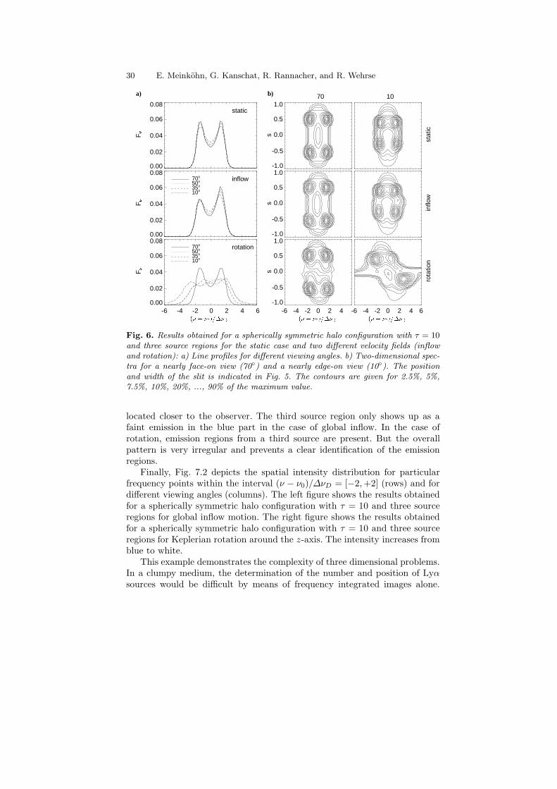
-6 -4 -2 0 2 4( 0)=D -6 -4 -2 0 2 4 6( 0)=DFig. 6. Results obtained for a spherically symmetric halo configuration with τ = 10and three source regions for the static case and two different velocity fields (inflowand rotation): a) Line profiles for different viewing angles. b) Two-dimensional spec-tra for a nearly face-on view (70) and a nearly edge-on view (10). The positionand width of the slit is indicated in Fig. 5. The contours are given for 2.5%, 5%,7.5%, 10%, 20%, ..., 90% of the maximum value.
located closer to the observer. The third source region only shows up as afaint emission in the blue part in the case of global inflow. In the case ofrotation, emission regions from a third source are present. But the overallpattern is very irregular and prevents a clear identification of the emissionregions.
Finally, Fig. 7.2 depicts the spatial intensity distribution for particularfrequency points within the interval (ν − ν0)/∆νD = [−2, +2] (rows) and fordifferent viewing angles (columns). The left figure shows the results obtainedfor a spherically symmetric halo configuration with τ = 10 and three sourceregions for global inflow motion. The right figure shows the results obtainedfor a spherically symmetric halo configuration with τ = 10 and three sourceregions for Keplerian rotation around the z-axis. The intensity increases fromblue to white.
This example demonstrates the complexity of three dimensional problems.In a clumpy medium, the determination of the number and position of Lyαsources would be difficult by means of frequency integrated images alone.
Multidimensional radiative transfer 31
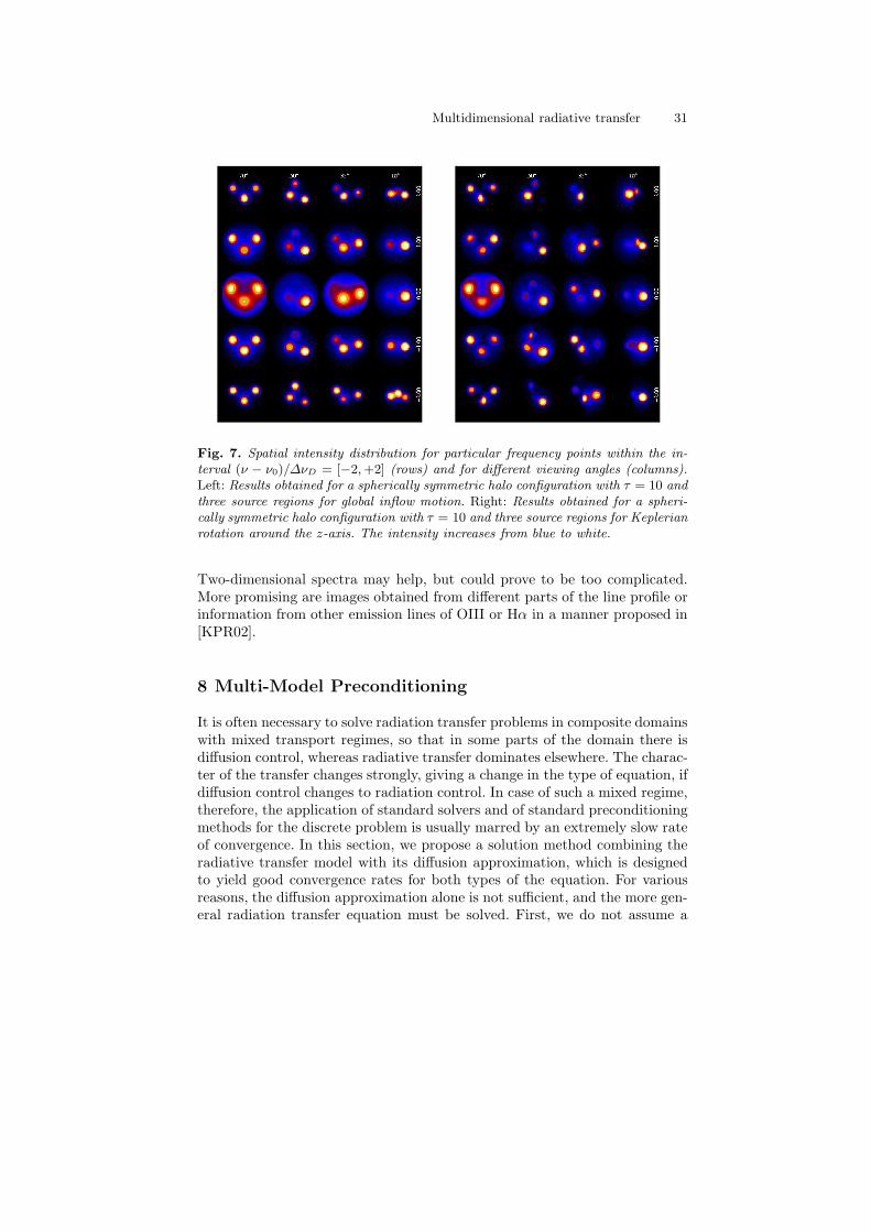
Fig. 7. Spatial intensity distribution for particular frequency points within the in-terval (ν − ν0)/∆νD = [−2, +2] (rows) and for different viewing angles (columns).Left: Results obtained for a spherically symmetric halo configuration with τ = 10 andthree source regions for global inflow motion. Right: Results obtained for a spheri-cally symmetric halo configuration with τ = 10 and three source regions for Keplerianrotation around the z-axis. The intensity increases from blue to white.
Two-dimensional spectra may help, but could prove to be too complicated.More promising are images obtained from different parts of the line profile orinformation from other emission lines of OIII or Hα in a manner proposed in[KPR02].
8 Multi-Model Preconditioning
It is often necessary to solve radiation transfer problems in composite domainswith mixed transport regimes, so that in some parts of the domain there isdiffusion control, whereas radiative transfer dominates elsewhere. The charac-ter of the transfer changes strongly, giving a change in the type of equation, ifdiffusion control changes to radiation control. In case of such a mixed regime,therefore, the application of standard solvers and of standard preconditioningmethods for the discrete problem is usually marred by an extremely slow rateof convergence. In this section, we propose a solution method combining theradiative transfer model with its diffusion approximation, which is designedto yield good convergence rates for both types of the equation. For variousreasons, the diffusion approximation alone is not sufficient, and the more gen-eral radiation transfer equation must be solved. First, we do not assume a
32 E. Meinkohn, G. Kanschat, R. Rannacher, and R. Wehrse
lower bound for the scattering cross section and, therefore, the approximationmay become inaccurate in parts of the domain. Furthermore, the questionarises as to what boundary conditions for the diffusion problem are physicallyacceptable. These problems can be fully resolved only by solving the radiativetransfer equation. Since the spectrum of the discrete operator becomes degen-erate in the limit when scattering dominates, the solution of the correspondingdiscrete linear system is particularly challenging (see [Kan96]).
When the parameters of the equation are constant, efficient solution tech-niques can be found easily. If scattering is small, a simple Gauss-Seidel processyields good convergence rates (see [JP86]). In the limit of high scattering, thesolution is isotropic in the interior of the domain yielding an elliptic second or-der equation, which can be solved efficiently using multilevel preconditioning.The scheme suggested in this section combines these two preconditioners in away related to two-level multigrid algorithms. It exploits the good convergenceproperties of both methods in different regimes. Similar schemes have beenproposed under the names of quasi diffusion and diffusion-synthetic accelera-tion method (for details see [Lar91, AL02] and the literature cited therein).
8.1 Discretization and Diffusion Approximation
Let us first consider monochromatic radiative transfer problems and rewritethe corresponding partial integro-differential equation (2) for a multidimen-sional spatial domain Ω ⊂ Rd (d = 2, 3)
n · ∇xI(x,n) = −χ(x)(I(x,n) − 1 − ǫ
2(d − 1)π
∫
Sd−1
I(x,n′) dω′ − ǫf(x)), (68)
with the thermalization factor ǫ = κ/χ and the albedo 1 − ǫ = σ/χ. For thesake of simplicity, isotropic scattering (i.e., phase function P (n′,n) ≡ 1), aconstant source function f(x) = 1 and – if not stated otherwise – zero bound-ary conditions are adopted. The test calculations which follow are exclusivelyperformed for 2D configurations (i.e., d = 2). For the discretization of theintegral operator in (68), a collocation method is used, again as described inSect. 4.2, using a set of equally spaced points on the unit circle. Then, thetransport equation (68) gives for an arbitrary fixed direction ni
ni · ∇xI(x,ni) + χ(x)I(x,ni) = χ(x)((1− ǫ)
k=m∑
k=1
ωikI(x,nk) + ǫf(x)), (69)
where the ωik are suitable quadrature weights with∑
k ωik = 1. Equation (69)is discretized by the discontinuous Galerkin finite element method (DGFEM)proposed for neutron transport without scattering in [LR74] and for radiativetransfer problems in [KM04]. Let Th be a mesh of quadrilaterals K coveringthe domain Ω exactly. On Th the finite element space Vh used for the specificintensity is defined by
Multidimensional radiative transfer 33
Vh =v ∈ L2(Th)
∣∣ v|K ∈ P , ∀K ∈ Th
. (70)
P is either the space of polynomials of degree k or the space of isoparametrictensor product polynomials of degree k on K. We assume k ≥ 1, yielding adiscretization of second order at least.
At large optical depths (χ ≫ 1) radiative transfer in scattering domi-nated media (ǫ → 0) becomes simple because all scale lengths become largerthan the photon mean free path length (∼ 1/χ(x)). Simple approximations tothis transport problem, based either on ad hoc physical assumptions such asFick’s law (cf. [Lam65, DL00]) or on a polynomial approximation, which as-sumes that the flux has an expansion into the first two Legendre Polynomials(cf. [CZ67]), result in a diffusion equation
−∇x ·(
1
dχ∇xJ(x)
)+ κJ(x) = κf(x) (71)
for the mean intensity J(x) = 1/(2(d − 1)π)∫
s2 I(x,n)dω. Usually, fixedboundary conditions of the type J(x) = g(x) are posed on the spatial bound-ary surface Γ . To derive the basic asymptotic (diffusion) limit for scatteringdominant, optically thick transport problems, the point x under considerationmust be far from the boundary (optical depth τ ≫ 1) and far from the zonesof the domain Ω where the coefficients κ and σ vary strongly. In the 1970s and1980s, the mathematical relationship between transport and diffusion theoryhas been clarified in a large body of work showing that transport theory tran-sitions into diffusion theory in a certain asymptotic limit. A sampling of thiswork is given in [LK74, HM75, Pap75, LPB83, LMM87]. As for the radiativetransfer equation (69) the DGFEM discretization of the diffusion equation(71) is achieved by the (symmetric) interior penalty method due to [Arn82]with polynomials of degree k ≥ 1, yielding a discretization of second-order atleast. The linear system of equations resulting from the DGFEM discretizationof Eq. (68) has the block structure
Adiff J = f . (72)
J is the vector of discrete mean intensities and f is any given data (thermalradiation and boundary data). The (n × n)-matrix Adiff corresponds to theDGFEM discretization of the left hand side of Eq. (71).
8.2 Preconditioning
The linear system of equations resulting from the DGFEM discretization ofEq. (68) has the block structure
A1
. . .
AM
−
ω11X · · · ω1MX
......
ωM1X · · · ωMMX
u1
...uM
=
f1
...fM
. (73)
34 E. Meinkohn, G. Kanschat, R. Rannacher, and R. Wehrse
Here, ui is the vector of discrete intensities and fi is any given data (ther-mal radiation and boundary data) for any fixed direction ni (i = 1, . . . , M).Each (n× n)-matrix Ai corresponds to the DGFEM discretization of the lefthand side of Eq. (69) for a single radiation direction ni and X discretizes themultiplication with (1 − ǫ)χ. The operator form of Eq. (73) reads
Arte u = f , (74)
where Arte = T − S is the pure transport operator T minus the scatteringoperator S.
Given a system of linear equations (74) and an iterate ui, the iteration
error is defined asei := u − ui. (75)
An equation for the error is given by the defect equation
Arte ei = Arte
(u − ui
)= f − Arte ui = di. (76)
An approximation g(x,n) for ei can be computed by solving
Mg = di ⇐⇒ g = M−1(f − Arte ui
). (77)
M should be an approximation of Arte that is easy to invert, such as:
M identity matrix (Richardson method)
M diagonal of Arte (Jacobi method)
M lower triangle of Arte (Gauss-Seidel method).
Now a new iterate is obtained by
ui+1 = ui + g. (78)
Renumbering the degrees of freedom according to the photon transportdirection ni, the matrices Ai in Eq. (73) can be inverted easily by a frontsolving algorithm (see [JP86]). Therefore, a simple, well-known preconditionerfor the system (73) is the matrix
Λ =
A−1
1
. . .
A−1
M
. (79)
It is this preconditioner, that is used in the well-known Λ- or Source Iterationmethod. Thus, with M ≡ Λ the new iterate in Eq. (78) reads
ui+1 = Λ
f +
ω11X · · · ω1MX
......
ωM1X · · · ωMMX
ui
. (80)
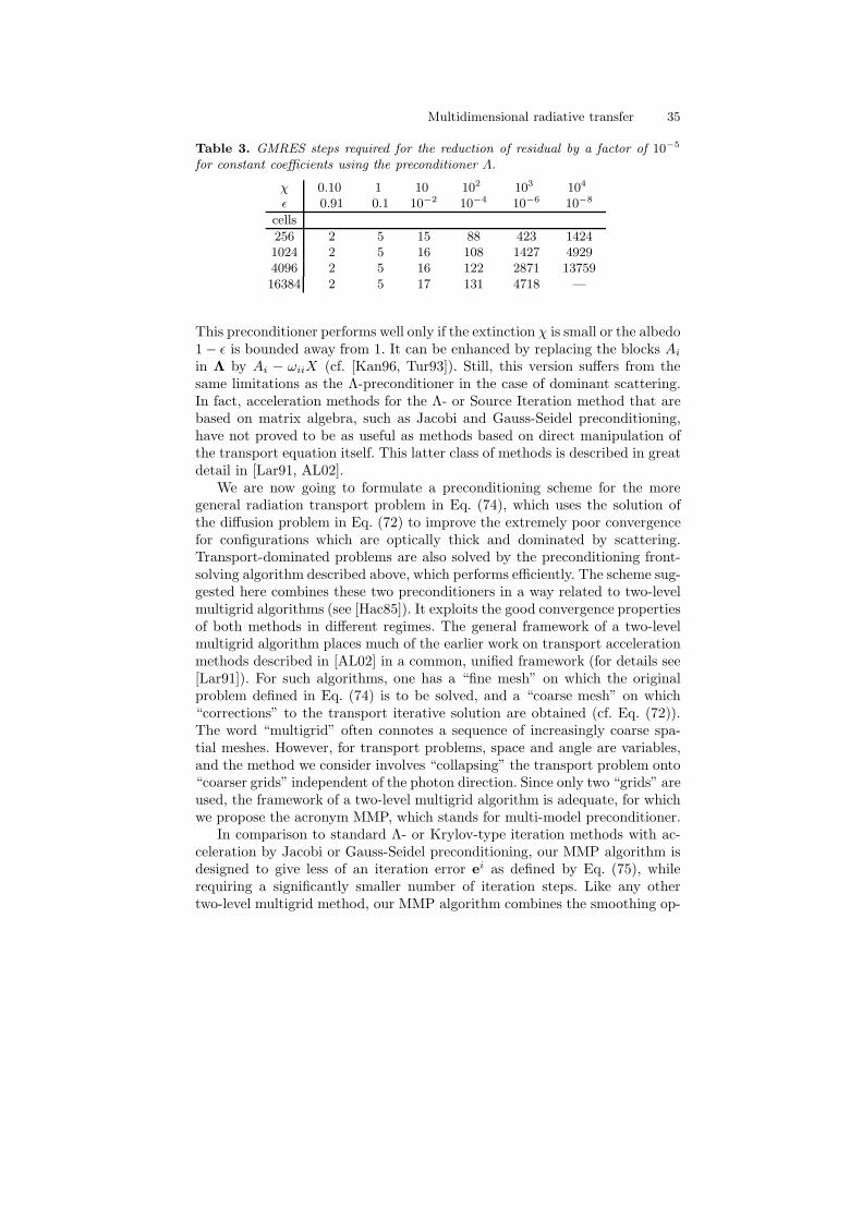
Multidimensional radiative transfer 35
Table 3. GMRES steps required for the reduction of residual by a factor of 10−5
for constant coefficients using the preconditioner Λ.
χ 0.10 1 10 102 103 104
ǫ 0.91 0.1 10−2 10−4 10−6 10−8
cells
256 2 5 15 88 423 14241024 2 5 16 108 1427 49294096 2 5 16 122 2871 1375916384 2 5 17 131 4718 —
This preconditioner performs well only if the extinction χ is small or the albedo1 − ǫ is bounded away from 1. It can be enhanced by replacing the blocks Ai
in Λ by Ai − ωiiX (cf. [Kan96, Tur93]). Still, this version suffers from thesame limitations as the Λ-preconditioner in the case of dominant scattering.In fact, acceleration methods for the Λ- or Source Iteration method that arebased on matrix algebra, such as Jacobi and Gauss-Seidel preconditioning,have not proved to be as useful as methods based on direct manipulation ofthe transport equation itself. This latter class of methods is described in greatdetail in [Lar91, AL02].
We are now going to formulate a preconditioning scheme for the moregeneral radiation transport problem in Eq. (74), which uses the solution ofthe diffusion problem in Eq. (72) to improve the extremely poor convergencefor configurations which are optically thick and dominated by scattering.Transport-dominated problems are also solved by the preconditioning front-solving algorithm described above, which performs efficiently. The scheme sug-gested here combines these two preconditioners in a way related to two-levelmultigrid algorithms (see [Hac85]). It exploits the good convergence propertiesof both methods in different regimes. The general framework of a two-levelmultigrid algorithm places much of the earlier work on transport accelerationmethods described in [AL02] in a common, unified framework (for details see[Lar91]). For such algorithms, one has a “fine mesh” on which the originalproblem defined in Eq. (74) is to be solved, and a “coarse mesh” on which“corrections” to the transport iterative solution are obtained (cf. Eq. (72)).The word “multigrid” often connotes a sequence of increasingly coarse spa-tial meshes. However, for transport problems, space and angle are variables,and the method we consider involves “collapsing” the transport problem onto“coarser grids” independent of the photon direction. Since only two “grids” areused, the framework of a two-level multigrid algorithm is adequate, for whichwe propose the acronym MMP, which stands for multi-model preconditioner.
In comparison to standard Λ- or Krylov-type iteration methods with ac-celeration by Jacobi or Gauss-Seidel preconditioning, our MMP algorithm isdesigned to give less of an iteration error ei as defined by Eq. (75), whilerequiring a significantly smaller number of iteration steps. Like any othertwo-level multigrid method, our MMP algorithm combines the smoothing op-
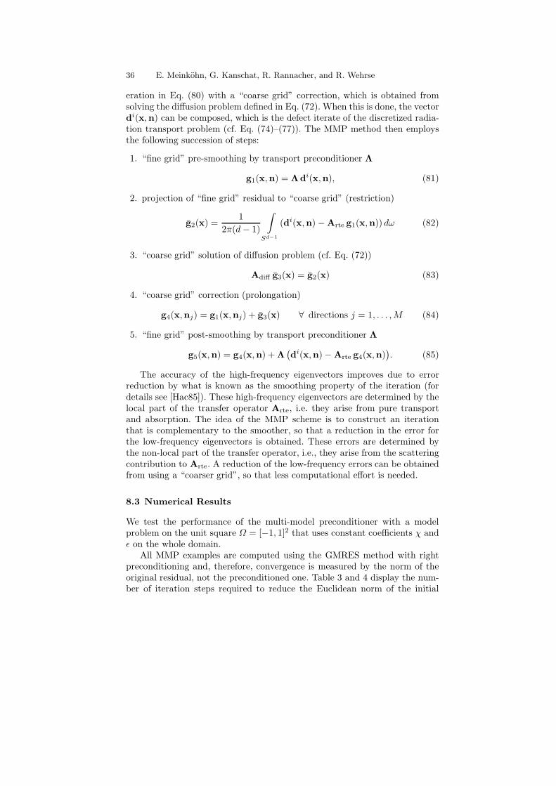
36 E. Meinkohn, G. Kanschat, R. Rannacher, and R. Wehrse
eration in Eq. (80) with a “coarse grid” correction, which is obtained fromsolving the diffusion problem defined in Eq. (72). When this is done, the vectordi(x,n) can be composed, which is the defect iterate of the discretized radia-tion transport problem (cf. Eq. (74)–(77)). The MMP method then employsthe following succession of steps:
1. “fine grid” pre-smoothing by transport preconditioner Λ
g1(x,n) = Λdi(x,n), (81)
2. projection of “fine grid” residual to “coarse grid” (restriction)
g2(x) =1
2π(d − 1)
∫
Sd−1
(di(x,n) − Arte g1(x,n)) dω (82)
3. “coarse grid” solution of diffusion problem (cf. Eq. (72))
Adiff g3(x) = g2(x) (83)
4. “coarse grid” correction (prolongation)
g4(x,nj) = g1(x,nj) + g3(x) ∀ directions j = 1, . . . , M (84)
5. “fine grid” post-smoothing by transport preconditioner Λ
g5(x,n) = g4(x,n) + Λ(di(x,n) − Arte g4(x,n)
). (85)
The accuracy of the high-frequency eigenvectors improves due to errorreduction by what is known as the smoothing property of the iteration (fordetails see [Hac85]). These high-frequency eigenvectors are determined by thelocal part of the transfer operator Arte, i.e. they arise from pure transportand absorption. The idea of the MMP scheme is to construct an iterationthat is complementary to the smoother, so that a reduction in the error forthe low-frequency eigenvectors is obtained. These errors are determined bythe non-local part of the transfer operator, i.e., they arise from the scatteringcontribution to Arte. A reduction of the low-frequency errors can be obtainedfrom using a “coarser grid”, so that less computational effort is needed.
8.3 Numerical Results
We test the performance of the multi-model preconditioner with a modelproblem on the unit square Ω = [−1, 1]2 that uses constant coefficients χ andǫ on the whole domain.
All MMP examples are computed using the GMRES method with rightpreconditioning and, therefore, convergence is measured by the norm of theoriginal residual, not the preconditioned one. Table 3 and 4 display the num-ber of iteration steps required to reduce the Euclidean norm of the initial
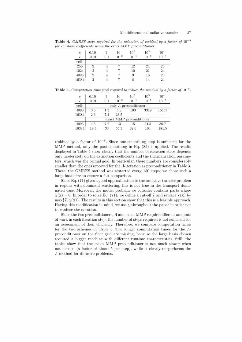
Multidimensional radiative transfer 37
Table 4. GMRES steps required for the reduction of residual by a factor of 10−5
for constant coefficients using the exact MMP preconditioner.
χ 0.10 1 10 102 103 104
ǫ 0.91 0.1 10−2 10−4 10−6 10−8
cells
256 2 4 7 12 24 261024 2 4 7 10 21 244096 2 4 7 9 16 2316384 2 4 7 8 14 24
Table 5. Computation time [sec] required to reduce the residual by a factor of 10−5.
χ 0.10 1 10 102 103 104
ǫ 0.91 0.1 10−2 10−4 10−6 10−8
cells only Λ preconditioner
4096 0.5 1.3 4.8 103 3319 1645716384 2.6 7.4 23.5 — — —
exact MMP preconditioner
4096 4.5 7.2 13 15 24.5 36.716384 19.4 33 55.3 62.6 104 181.5
residual by a factor of 10−5. Since one smoothing step is sufficient for theMMP method, only the post-smoothing in Eq. (85) is applied. The resultsdisplayed in Table 4 show clearly that the number of iteration steps dependsonly moderately on the extinction coefficients and the thermalization parame-ters, which was the primal goal. In particular, these numbers are considerablysmaller than the ones reported for the Λ-iteration as preconditioner in Table 3.There, the GMRES method was restarted every 150 steps; we chose such alarge basis size to ensure a fair comparison.
Since Eq. (71) gives a good approximation to the radiative transfer problemin regions with dominant scattering, this is not true in the transport domi-nated case. Moreover, the model problem we consider contains parts whereχ(x) = 0. In order to solve Eq. (71), we define a cut-off χ and replace χ(x) bymaxχ, χ(x). The results in this section show that this is a feasible approach.Having this modification in mind, we use χ throughout the paper in order notto confuse the notation.
Since the two preconditioners, Λ and exact MMP require different amountsof work in each iteration step, the number of steps required is not sufficient foran assessment of their efficiency. Therefore, we compare computation timesfor the two schemes in Table 5. The longer computation times for the Λ-preconditioner on the finer grid are missing, because the large basis chosenrequired a bigger machine with different runtime characteristics. Still, thetables show that the exact MMP preconditioner is not much slower whennot needed (a factor of about 5 per step), while it clearly outperforms theΛ-method for diffusive problems.
38 E. Meinkohn, G. Kanschat, R. Rannacher, and R. Wehrse
9 Summary
A finite element code for solving the resonance line transfer problem in movingmedia is presented. Simple velocity fields and complete redistribution are con-sidered. The code is applicable to any three-dimensional model configurationwith optical depths up to 103–104.
The application to the hydrogen Lyα line originating from slightly opticallythick model configurations (τ ≤ 102) are shown and the resulting line profilesare discussed in detail. The systematic approach from very simple to morecomplex models gave the following results:
• An optical depth of τ ≥ 1 leads to the characteristic double peaked lineprofile with a central absorption trough as expected from analytical studies(e.g., see [Neu90]). This form of the profile is the result of scattering inspace and frequency. Photons escape via the line wings where the opticaldepth is much lower.
• Global velocity fields destroy the symmetry of the line profile. Generally,the blue peak of the profile is enhanced for models simulating a collapsemotion and the red peak for expanding media. But there are certain ve-locity fields (e.g. with steep gradients) and spatial distributions of theextinction coefficient, where the formation of a prominent peak is sup-pressed.
• Double-peaked line-profiles show up as two emission regions in the two-dimensional spectra. Global collapse or expansion leads to an overall tri-angular shape of the emission. Rotation produces a shear pattern resultingin banana-shaped emission regions for optical depths ≥ 10.
• For non-symmetrical model configurations, the optical depth varies withthe line of sight. Thus, the flux, the depth of the absorption trough andthe pattern in the two-dimensional spectra strongly depend on the viewingdirection.
The applications clearly demonstrate the capacity of the finite elementcode and show that the three-dimensional structure, the kinematics and thetotal optical depth of the model configurations are very important. The lat-ter point is crucial, since the convergence of the algorithm is extremely poorfor optical depths ≥ 103 − 104. These large depths refer to photons at theline center. Photons in the line wings or those emerging close to the bound-ary of the halo configuration hardly interact with the cold hydrogen gas andwill escape almost freely towards the observer. These objects are especiallychallenging from a numerical point of view. They are simulated by the multi-model preconditioning (MMP) scheme presented in this paper, which com-bines two distinct preconditioners that are designed to accelerate the solutionof transport dominated and highly scattering, optically thick radiative trans-fer problems. The development of the MMP method was stimulated by thetheory of two-level multigrid algorithms which exploit the good convergenceproperties of both transport and scattering acceleration methods in different
Multidimensional radiative transfer 39
spatial regimes. The monochromatic model problems clearly demonstrate theconsiderable improvement in run-time efficiency of the MMP scheme.
References
[Ada72] Adams, T.F.: The escape of resonance-line radiation from extremelyopaque media. Astrophys. J., 174, 439 (1972)
[AL02] Adams, M.L., Larsen, E.W.: Fast iterative methods for discrete-ordinatesparticle transport calculations. Prog. Nucl. Energy, 40, No. 1, 3–159 (2002)
[ALL01] Ahn, S.-H., Lee, H.-W., Lee, H. M.: Lyα line formation in starburst galax-ies. I. Moderately thick, dustless and static H I media. Astrophys. J., 554,604–614 (2001)
[ALL02] Ahn, S.-H., Lee, H.-W., Lee, H. M.: Lyα line formation in starburst galax-ies. II. Extremely thick, dustless and static H I media. Astrophys. J., 567,922–930 (2002)
[Arn82] Arnold, D.N.: An interior penalty finite element method with discontinu-ous elements. SIAM J. Numer. Anal., 19, 742–760 (1982)
[BR01] Becker, R., Rannacher, R.: An optimal control approach to a posteriorierror estimation in finite element methods. In: Iserles, A. (ed.) Acta Nu-merica 2001, 37, p. 1–102, Cambridge University Press (2001)http://www.iwr.uni-heidelberg.de/sfb359/Preprints2001.html
[BBR05] Becker, R., Braack, M., Richter, T.: Parallel multigrid on locally refinedmeshes. In: Rannacher, R. (ed.) Reactive Flows, Diffusion and Transport.Springer, Berlin (2005)
[BKM05] Becker, R., Kapp, H., Meidner, D., Rannacher, R., Vexler, B.: Adaptivefinite element methods for PDE-constrained optimal control problems. In:Rannacher, R. (ed.) Reactive Flows, Diffusion and Transport. Springer,Berlin (2005)
[Boe96] Bottcher K.: Adaptive Schrittweitenkontrolle beim Unstetigen Galerkin-Verfahren fur Gewohnliche Differentialgleichungen. Diploma Thesis, Uni-versity of Heidelberg (1996)
[BR05a] Braack, M., Richter, T.: Mesh and model adaptivity for flow problems. In:Rannacher, R. (ed.) Reactive Flows, Diffusion and Transport. Springer,Berlin (2005)
[BR05b] Braack, M., Richter, T.: Solving multidimensional reactive flow problemswith adaptive finite elements. In: Rannacher, R. (ed.) Reactive Flows,Diffusion and Transport. Springer, Berlin (2005)
[Bra97] Braess, D.: Finite Elemente. Springer, Berlin (1997)[BH71] Bramble, J.H.,Hilbert, S.R.: Bounds for a class of linear functionals with
applications to Hermite interpolation. Numer. Math., 16, 362–369 (1971)[BS96] Brenner, S.C., Scott, L.R.: The Mathematical Theory of Finite Element
Methods. Springer, New York (1996)[CHR05] Carraro, T., Heuvelin, V., Rannacher, R., Waguet, C.: Determination of
kinetic parameters in laminar flow reactors. I. Numerical aspects. In: Ran-nacher, R. (ed.) Reactive Flows, Diffusion and Transport. Springer, Berlin(2005)
[CZ67] Case, K.M., Zweiffel, P.F.: Linear Transport Theory. Addison-WesleyPublishing Company, Reading, Massachusetts (1967)
40 E. Meinkohn, G. Kanschat, R. Rannacher, and R. Wehrse
[Cia78] Ciarlet, P.G.: The Finite Element Method for Elliptic Problems. NorthHolland, New York (1978)
[DL00] Dautray R., Lions J.-L.: Mathematical Analysis and Numerical Methodsfor Science and Technology. Vol. 6, Springer, Berlin Heidelberg New York(2000)
[BRM00] De Breuck, C., Rottgering, H., Miley, G., van Breugel, W., Best, P.: Astatistical study of emission lines from high redshift radio galaxies. Astron.Astrophys., 362, 519–543 (2000)
[DT00] Dullemond, C.P., Turolla, R.: An efficient algorithm for two-dimensionalradiative transfer in axisymmetric circumstellar envelopes and disks. As-tron. Astrophys., 360, 1187–1202 (2000)
[ER90] Efstathiou, A., Rowan-Robinson, M.: Radiative transfer in axisymmetricdust clouds. Mon. Not. Roy. Astron. Soc., 245, 275–288 (1990)
[EJT85] Eriksson K., Johnson C., Thomee C.: Time discretization of parabolicproblems by the discontinuous Galerkin method. RAIRO, ModelisationMath. Anal. Numer., 19, 611–643 (1985)
[EJ87] Eriksson K., Johnson C.: Error estimates and automatic time step controlfor nonlinear parabolic problems. I. SIAM J. Numer. Anal., 24, 12–23(1987)
[EJ91] Eriksson K., Johnson C.: Adaptive finite element methods for parabolicproblems. I: A linear model problem. SIAM J. Numer. Anal., 28, 43–77(1991)
[FK97] Fuhrer C., Kanschat G.: A posteriori error control in radiative transfer.Computing, 58, 317–334 (1997)
[HM91] Haardt, F., Maraschi, L.: A two-phase model for the X-ray emission fromSeyfert galaxies. Astrophys. J., 380, L51–L54 (1991)
[HM75] Habetler, G.J., Matkowsky, B.J.: Uniform asymptotic expansions in trans-port theory with small mean free paths, and the diffusion approximation.J. Math. Phys., 16, 846–854 (1975)
[Hac85] Hackbusch, W.: Multi-Grid Methods and Applications. Springer, Heidel-berg (1985)
[Hac93] Hackbusch, W.: Iterative Losung Grosser Schwachbesetzter Gle-ichungssysteme. Teubner, Stuttgart (1993)
[Hog98] Hogerheijde, M.: The Molecular Environment of Low-Mass Protostars.Ph.D. Thesis, Rijks Univesiteit Leiden (1998)
[HB82] Hughes, T.J.R., Brooks, A.N.: Streamline upwind/Petrov-Galerkin for-mulations for convection dominated flows with particular emphasis on theincompressible Navier-Stokes equations. Comput. Methods Appl. Mech.Eng., 32, 199–259 (1982)
[HK80] Hummer, D.G., Kunasz, P.B.: Energy loss by resonance line photons inan absorbing medium. Astrophys. J., 236, 609–618 (1980)
[Joh87] Johnson, C.: Numerical Solution of Partial Differential Equations by theFinite Element Method. Cambridge University Press, Cambridge (1987)
[JP86] Johnson, C., Pitkaranta, J.: An analysis of the discontinuous Galerkinmethod for a scalar hyperbolic equation. Math. Comput., 46, 1–26 (1986)
[Juv97] Juvela, M.: Non-LTE radiative transfer in clumpy molecular clouds. As-tron. Astrophys., 322, 943–961 (1997)
[Kan96] Kanschat, G.: Parallel and Adaptive Galerkin Methods for RadiativeTransfer Problems. Ph.D. Thesis, University of Heidelberg (1996)http://www.iwr.uni-heidelberg.de/sfb359/Preprints1996.html
Multidimensional radiative transfer 41
[Kan00] Kanschat, G.: Solution of multi-dimensional radiative transfer problemson parallel computers. In: Bjorstad P. and Luskin M. (eds.) Parallel So-lution of PDE, IMA Vol. in Math. and its Appl., 120, Springer, BerlinHeidelberg New York, 85–96 (2000)
[KM04] Kanschat, G., Meinkohn, E.: Multi-model preconditioning for radiativetransfer problems. Preprint SFB 359, University of Heidelberg (2004)http://www.sfb359.uni-heidelberg.de/Preprints2004.html
[KPR02] Kurk, J.D., Pentericci, L., Rottgering, H.J.A., Miley, G.K.: Observationsof radio galaxy MRC 1138-262: Merging galaxies embedded in a giant Lyαhalo. In: Henney, W.J., Steffen, W., Raga, A.C., Binette, L. (eds) EmissionLines from Jet Flows. RMxAA (Serie de Conferencias), Vol. 13, 191–195(2002)
[Lam65] Lamarsh, J.R.: Introduction to Nuclear Reactor Theory. Addison-WesleyPublishing Company, Reading, Massachusett (1965)
[LK74] Larsen, E.W., Keller, J.B.: Asymptotic solution of neutron transport prob-lems for small scale mean free paths. J. Math. Phys., 15, 75–81 (1974)
[LPB83] Larsen, E.W., Pomraning, G.C., Badham, V.C.: Asymptotic analysis ofradiative transfer problems. J. Quant. Spectrosc. Radiat. Transfer, 29,285–310 (1983)
[LMM87] Larsen, E.W., Morel, J.E., Miller, W.F.jun.: Asymptotic solutions of nu-merical transport problems in optically thick, diffusive regimes. J. Comput.Phys., 69, 283–324 (1987)
[Lar91] Larsen, E.W.: Transport acceleration methods as two-level multigrid algo-rithms. Oper. Theory, Adv. Appl., 51, 34–47 (1991)
[LR74] LeSaint, P., Raviart, P.-A.: On a finite element method for solving theneutron transport equation. In: de Boor (ed.) Mathematical Aspects ofFinite Elements in Partial Differential Equations. Academic Press, NewYork, 89–123 (1974)
[MR02] Meinkohn, E., Richling, S.: Radiative transfer with finite elements. II. Lyαline transfer in moving media. Astron. Astrophys., 392, 827–839 (2002)
[Mei02] Meinkohn, E.: Modeling Three-Dimensional Radiation Fields in the EarlyUniverse. Ph.D. Thesis, University of Heidelberg (2002)http://www.iwr.uni-heidelberg.de/sfb359/Preprints2002.html
[Mih78] Mihalas, D.: Stellar Atmospheres. W.H. Freeman and Company, SecondEdition, San Francisco (1978)
[MW84] Mihalas, D., Weibel-Mihalas, B.: Foundation of Radiation Hydrodynam-ics. Oxford University Press, New York (1984)
[MCK94] Murray, S., Castor, J., Klein, R., McKee, C.: Accretion disk coronae inhigh-luminosity systems. Astrophys. J., 435, 631–646 (1994)
[Neu90] Neufeld, D.A.: The transfer of resonance-line radiation in static astro-physical media. Astrophys. J., 350, 216–241 (1990)
[Pap75] Papanicolaou, G.C.: Asymptotic analysis of transport processes. Bull. Am.Math. Soc., 81, 330–392 (1975)
[PH98] Park, Y.-S., Hong, S.S.: Three-dimensional Non-LTE Radiative Transferof CS in Clumpy Dense Cores. Astrophys. J., 494, 605 (1998)
[PSS79] Pozdniakov, L.A., Sobol, I.M., Suniaev, R.A.: The profile evolution ofX-ray spectral lines due to Comptonization - Monte Carlo computations.Astron. Astrophys., 75, 214–222 (1979)
42 E. Meinkohn, G. Kanschat, R. Rannacher, and R. Wehrse
[RM01] Richling, S., Meinkohn, E., Kryzhevoi, N., Kanschat, G.: Radiative trans-fer with finite elements. I. Basic method and tests. Astron. Astrophys.,380, 776–788 (2001)
[SF93] Sleijpen, G.L.G., Fokkema, D.R.: Bicgstab(L) for linear equations involv-ing unsymmetric matrices with complex spectrum. Electronic Transactionson Numerical Analysis, Vol. 1, 11–32 (1993)http://etna.mcs.kent.edu
[SPY95] Sonnhalter, C., Preibisch, T., Yorke, H.: Frequency dependent radiationtransfer in protostellar disks. Astron. Astrophys., 299, 545 (1995)
[Spa96] Spaans, M.: Monte Carlo models of the physical and chemical propertiesof inhomogeneous interstellar clouds. Astron. Astrophys., 307, 271 (1996)
[SL87] Spagna Jr., G.F., Leung, C.M.: Numerical solution of the radiation trans-port equation in disk geometry. J. Quant. Spectrosc. Radiat. Transfer, 37,565–580 (1987)
[SAS00] Steidel, C.C., Adelberger, K.L., Sharply, A.E., Pettini, M., Dickinson,M., Giavalisco, M.: Lyα Imaging of a Proto-Cluster Region at ¡z¿=3.09.Astrophys. J., 532, 170–182 (2000)
[SSW91] Stenholm, L.G., Storzer, H., Wehrse, R.: An efficient method for the so-lution of 3-D radiative transfer problems. J. Quant. Spectrosc. Radiat.Transfer, 45, 47–56 (1991)
[Tur93] Turek, S.: An efficient solution technique for the radiative transfer equa-tion. Imp. Comput. Sci. Eng., 5, No. 3, 201–214 (1993)
[ORM97] van Ojik, R., Rottgering, H.J.A., Miley, G.K., Hunstead, R.W.: The na-ture of the extreme kinematics in the extended gas of high redshift radiogalaxies. Astron. Astrophys., 317, 358–384 (1997)
[Var00] Varga, R.S.: Matrix Iterative Analysis. Springer, Berlin Heidelberg (2000)[WWM04] Warsa, J.S., Wareing, T.A., Morel, J.E.: Krylov Iterative Methods and
the Degraded Effectiveness of Diffusion Synthetic Acceleration for Multi-dimensional Sn Calculations in Problems with Material Discontinuities.Nucl. Sci. Eng., 147, 218–248 (2004)
[WMK99] Wehrse R., Meinkohn E., Kanschat G.: A review of Heidelberg radia-tive transfer equation solutions. In: Stee P. (ed.) Radiative Transfer andHydrodynamics in Astrophysics. EAS Publication Series, Vol. 5, 13–30(2002)
[WBW00] Wehrse R., Baschek B., von Waldenfels, W.: The diffusion of radiationin moving media: I. Basic assumptions and formulae. Astron. Astrophys.,359, 780–787 (2000)
[WHS99] Wolf, S., Henning, T., Stecklum, B.: Multidimensional self-consistent ra-diative transfer simulations based on the Monte-Carlo method. Astron.Astrophys., 349, 839–850 (1999)
[YBL93] Yorke, H., Bodenheimer, P., Laughlin, G.: The formation of protostellardisks. I - 1 M(solar). Astrophys. J., 411, 274–284 (1993)
[ZM02] Zheng, Z., Miralda-Escude, J.: Monte Carlo simulation of Lyα scatteringand application to damped Lyα systems. Astrophys. J., 578, 33–42 (2002)