Física estatística do crime: leis de escala...

Física estatística do crime: leis de escala e

redes complexasLuiz G. A. Alves, Ph.D.

Universidade de São Paulo

@lgaalves

\

The previous quantity explicitly considers the allometry between an urban indicator and thepopulation size, creating a relative measure that is not biased by the population size (size-inde-pendent) for any value of βi. The scale-adjusted metric DYi

(t) captures the exceptionality (eithergood or bad) of a city, which somehow is the result of the nonlinear agglomeration process

Table 1. Allometric relationships between urban indicators and population size. Values of parametersAiand βiobtained via orthogonal distanceregression on the relationship between logYi(t) and logN(t) for each urban indicator in the year t (see Methods Section). The values inside the brackets arethe standard errors (SE) in the last decimal of the estimated parameters. The last column shows the values of the Pearson linear correlation coefficient ρ foreach allometry in log-log scale.

Indicator Yi(t) Year t Ai (SE) βi (SE) ρ

Child labor 1991 −0.64 (5) 0.96 (1) 0.909

2000 −0.55 (5) 0.93 (1) 0.906

2010 −0.80 (5) 0.95 (1) 0.884

Elderly population 1991 −0.99 (5) 0.992 (6) 0.976

2000 −0.83 (2) 0.969 (5) 0.980

2010 −0.72 (2) 0.963 (5) 0.982

Female population 1991 −0.367 (3) 1.014 (1) 1.000

2000 −0.361 (2) 1.013 (1) 1.000

2010 −0.355 (2) 1.012 (1) 1.000

Homicides 1991 −5.4 (1) 1.35 (3) 0.769

2000 −5.7 (1) 1.41 (2) 0.800

2010 −5.04 (9) 1.29 (2) 0.827

Illiteracy 1991 −0.29 (7) 0.92 (2) 0.789

2000 −0.26 (7) 0.87 (2) 0.774

2010 −0.28 (7) 0.85 (2) 0.749

Family income 1991 0.82 (6) 0.33 (1) 0.428

2000 1.14 (6) 0.31 (1) 0.440

2010 1.63 (5) 0.23 (1) 0.440

Male population 1991 −0.239 (3) 0.987 (1) 1.000

2000 −0.243 (2) 0.987 (1) 1.000

2010 −0.249 (2) 0.988 (1) 1.000

Unemployment 1991 −3.50 (8) 1.45 (2) 0.880

2000 −2.07 (5) 1.25 (1) 0.940

2010 −2.09 (5) 1.20 (1) 0.931

doi:10.1371/journal.pone.0134862.t001

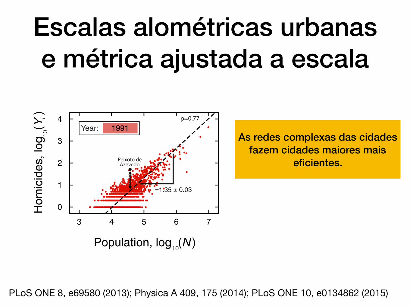
Fig 2. Allometric laws and the definition of the scale-adjustedmetricDYi(t). The scatter plots show the allometric relationships between number of

homicides and population size for the years t = 1991, 2000 and 2010 in log-log scale (see S1 and S2 Figs for all other indicators). The allometric exponents βi(see Methods Section for details on the calculation of βi) and Pearson correlation coefficient ρ are shown in the figures. We highlight a particular city (Peixotode Azevedo) in the three years to illustrate the definition and the evolution DYi

(t). For this city, the number homicides was quite above the allometric law in theyear t = 1991; however, it has approached the expected value by the allometric law over the years.

doi:10.1371/journal.pone.0134862.g002

Scale-Adjusted Metrics for Quantifying the Performance of Cities

PLOS ONE | DOI:10.1371/journal.pone.0134862 September 10, 2015 5 / 17

The previous quantity explicitly considers the allometry between an urban indicator and thepopulation size, creating a relative measure that is not biased by the population size (size-inde-pendent) for any value of βi. The scale-adjusted metric DYi

(t) captures the exceptionality (eithergood or bad) of a city, which somehow is the result of the nonlinear agglomeration process

Table 1. Allometric relationships between urban indicators and population size. Values of parametersAiand βiobtained via orthogonal distanceregression on the relationship between logYi(t) and logN(t) for each urban indicator in the year t (see Methods Section). The values inside the brackets arethe standard errors (SE) in the last decimal of the estimated parameters. The last column shows the values of the Pearson linear correlation coefficient ρ foreach allometry in log-log scale.

Indicator Yi(t) Year t Ai (SE) βi (SE) ρ

Child labor 1991 −0.64 (5) 0.96 (1) 0.909

2000 −0.55 (5) 0.93 (1) 0.906

2010 −0.80 (5) 0.95 (1) 0.884

Elderly population 1991 −0.99 (5) 0.992 (6) 0.976

2000 −0.83 (2) 0.969 (5) 0.980

2010 −0.72 (2) 0.963 (5) 0.982

Female population 1991 −0.367 (3) 1.014 (1) 1.000

2000 −0.361 (2) 1.013 (1) 1.000

2010 −0.355 (2) 1.012 (1) 1.000

Homicides 1991 −5.4 (1) 1.35 (3) 0.769

2000 −5.7 (1) 1.41 (2) 0.800

2010 −5.04 (9) 1.29 (2) 0.827

Illiteracy 1991 −0.29 (7) 0.92 (2) 0.789

2000 −0.26 (7) 0.87 (2) 0.774

2010 −0.28 (7) 0.85 (2) 0.749

Family income 1991 0.82 (6) 0.33 (1) 0.428

2000 1.14 (6) 0.31 (1) 0.440

2010 1.63 (5) 0.23 (1) 0.440

Male population 1991 −0.239 (3) 0.987 (1) 1.000

2000 −0.243 (2) 0.987 (1) 1.000

2010 −0.249 (2) 0.988 (1) 1.000

Unemployment 1991 −3.50 (8) 1.45 (2) 0.880

2000 −2.07 (5) 1.25 (1) 0.940

2010 −2.09 (5) 1.20 (1) 0.931

doi:10.1371/journal.pone.0134862.t001

Fig 2. Allometric laws and the definition of the scale-adjustedmetricDYi(t). The scatter plots show the allometric relationships between number of

homicides and population size for the years t = 1991, 2000 and 2010 in log-log scale (see S1 and S2 Figs for all other indicators). The allometric exponents βi(see Methods Section for details on the calculation of βi) and Pearson correlation coefficient ρ are shown in the figures. We highlight a particular city (Peixotode Azevedo) in the three years to illustrate the definition and the evolution DYi

(t). For this city, the number homicides was quite above the allometric law in theyear t = 1991; however, it has approached the expected value by the allometric law over the years.




Escalas alométricas urbanas e métrica ajustada a escala

PLoS ONE 8, e69580 (2013); Physica A 409, 175 (2014); PLoS ONE 10, e0134862 (2015)

As redes complexas das cidades fazem cidades maiores mais

eficientes.

In addition of being autocorrelated with their past values, DYi(t + Δt) for the urban indicator

ialso displays statistically significant crosscorrelations with DYj(t) for other indicators j (S4

Fig). These memory effects and also the fact that the residuals surrounding the relationshipsDYi

(t + Δt) versus DYi(t) are very close to Gaussian distributions (S5 Fig) with standard devia-

tions across windows practically constant (S6 Fig) make these scale-adjusted metrics particu-larly good for being used in linear regressions aiming forecasts. We have thus adjusted thelinear model (via ordinary least-squares method)

DYiðt þ DtÞ ¼ C0 þ

X8

k¼ 1

Ck DYkðtÞ þ ZiðtÞ ð6Þ

by considering the relationships (t + Δt) = 2000 versus t = 1991 and (t + Δt) = 2010 versust = 2000. In Eq 6, Ck is the linear coefficient quantifying the predictive power of DYk

(t) on DYi(t

+ Δt) (C0 is the intercept coefficient) and ηi(t) is the noise term accounting for the effect ofunmeasurable factors. The results exhibiting the linear coefficients of each linear regression forthe two combinations of years are shown in S1 Text. We note that these simple models accountfor 31%–97% of the observed variance in DYi

(t + Δt) and that they correctly reproduce the aver-age values of the scale-adjusted metric above and below the allometric laws for the years 2000and 2010 only using data from the years 1991 and 2000, respectively (see S7 Fig). We have fur-ther compared the distributions of the empirical values of DYi

with the predictions of these lin-ear models and observed that the agreement is remarkable good for the indicators elderly,female and male population as well as for illiteracy and income (S8and S9 Figs). Motivated bythese good agreements, we proposed to forecast the values of DYi

(t + Δt) in the year of 2020(next Brazilian national census). In order to do so, we have considered that the linear coeffi-cients Ck are constant over time and employed the average value of Ck over the two combina-tions of years used in Eq 6 for predicting the values of DYi

(t + Δt). It is worth noting that byassuming Ck constant, we are ignoring the evolution of socio-economic and policy factors. Inan ideal scenario, one could track the evolution of the values of Ck for achieving more reliablepredictions. However, our data (that is, the two values for Ck) do not enable us to probe possi-ble evolutionary behaviors in the values of Ck. Even so, as pointed by Bettencourt [6], thedynamics of the urban metrics seems to be dominated by long timescales (* 30 years), andthus the approach of constant coefficients should be seen as a first approximation. The graysbars in Fig 3 show the averages DYi

(2020) after grouping the cities with DYi(1991)> 0 and

DYi(1991)< 0. We observe that predictions for the average values basically keep the trends pre-

sented in the previous years; for unemployment, in which the trend was not very clear, the pre-dictions put this indicator together with most indicators, where the average DYi

(t) has beendecreasing for cities initially above the allometric law and increasing for those initially below.

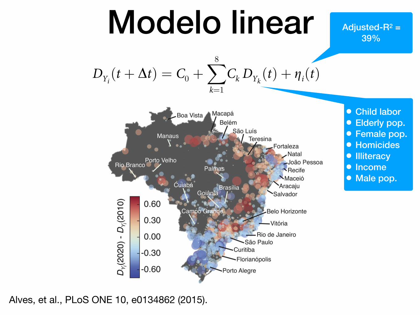
In order to gain further information on the predictions, we build a geographic visualizationof the expected changes in DYi

(t) between the years t = 2010 and t = 2020. The circles over themaps in Fig 5 show the geographic location of Brazilian cities; the radii of these circles are pro-portional to jDYi

(2020) − DYi(2010)j and are colored with shades of azure for cities where

[DYi(2020) − DYi

(2010)]< 0 (the indicator is expected to decrease) and with shades of red forcities where [DYi

(2020) − DYi(2010)]> 0 (the indicator is expected to increase); in both cases,

the darker the shade, the larger is the absolute value of the difference [DYi(2020) − DYi

(2010)].Perhaps, the most striking feature of these visualizations is the fact that the predicted changesappear spatially clustered for almost all indicators, which somehow reflects the geographicinequalities existing in Brazil; however, some intriguing patterns are indicator-dependent.

For child labour, DYi(t) is expected to increase around three of the most densely populated

regions that contain the metropolitan areas of São Paulo, Rio de Janeiro and the metropolitan



areas of almost all northeast capitals; we further observe that a decrease in child labour cases isexpected in mostly of the inner and southern cities. For the indicators elderly, female and malepopulations the clustering of the changes in DYi

(t) is quite evident: elderly and female popula-tions are foreseen to decrease in mostly of the northeast cities and display an increasing

Fig 5. Geographic visualization of the predicted changes in the scale-adjusted metricsDYi(t) between the years t = 2010 and t = 2020. Each circle

represents a city and the radius of the circle is proportional to jDYi(2020) − DYi

(2010)j. We color the circles according to the difference between DYi(2020) and

DYi(2010): shades of azure indicate that we expect a decrease in the values of DYi

(2020), whereas shades of red show the cities where we expect an increasein the values of DYi

(2020). The labeled cities are the capitals of the twenty-seven Federal Units of Brazil (the Brazilian states and the federal district). Theforecast for the values of DYi

(2020) were obtained through the linear model of Eq 6, where the linear coefficientCk were averaged over the two combinationsof years 2000—1991 and 2010—2000. We note that the changes in DYi

(t) appear spatially clustered for most indicators, forming regions where most citiesare expected to increase or decrease the value of the scale-adjusted metric.




Alves, et al., PLoS ONE 10, e0134862 (2015).

Modelo linear Adjusted-R2 = 39%

• Child labor • Elderly pop. • Female pop. • Homicides • Illiteracy • Income • Male pop.

Alves, et al. (2018), Physica A 505, 435–443

the variables in a stepwise fashion or considering non-linear models (e.g., the negative binomial138

regression) to overcome some of these problems. Unfortunately, in the literature we often find139

results based on simple OLS linear regression approach, which can mislead the conclusions about140

the causes of crime. We could further explore and check for other inconsistencies in this linear141

regression approach and fix them along the way using the several approaches proposed in the142

literature of linear regression [57]. Nevertheless, we now focus on an alternative approach to143

overcome these limitations and having a meaningful rank of features under slight changes in the144

dataset. Our proposed approach are much more flexible about the requirements of the data and in145

fact, no transformation or data preparation is needed to achieve a good result regarding accuracy146

in the predictions and interpretability of the results.147

2.3. Random forest algorithm148

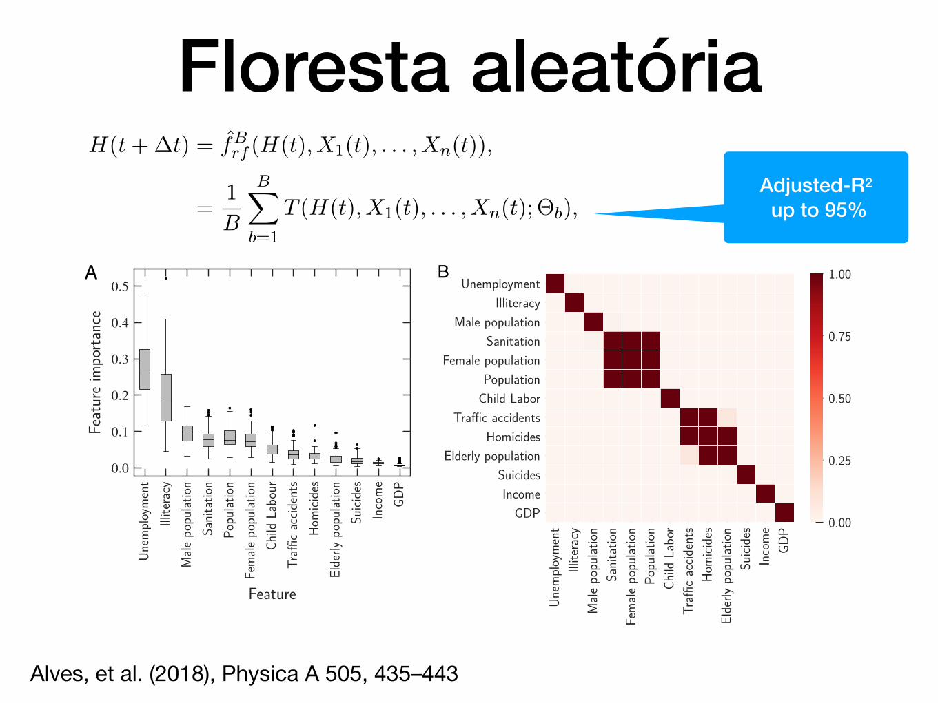
Random forest is an ensemble learning method used for classification or regression that fits149

several decision trees using various sub-samples of the dataset and aggregate their individual pre-150

dictions to form a final output and reduce overfitting [58, 46, 47, 48, 49]. In the random forest re-151

gression, several independent decision trees are constructed by a bootstrap sampling of the dataset.152

The final output is the result of a majority voting among the trees (estimators) or the average over153

all trees. The process of “bagging features” selects more often the best metrics to describe the154

data splits, and consequently, make them more important on the majority voting [52]. Unlike usual155

linear models, the random forest is invariant under scaling and various other transformations of the156

feature values. It is also robust to the inclusion of irrelevant features and produces very accurate157

predictions [47]. These properties of the random forest algorithm make it especially suitable for158

crime forecasting, because of the multicollinearity and non-linearities present in urban data.159

Considering the random forest regressor, the model from Eq. 1 can be rewritten as160

H(t+�t) = f̂Brf (H(t), X1(t), . . . , Xn(t)),

=1

B

BX

b=1

T (H(t), X1(t), . . . , Xn(t);⇥b),(2)

where each tree T adjust the data using the parameters given by ⇥b, which in turn characterizes161

the b-th random forest tree in terms of split variables, cutpoints at each node, and terminal-node162

values [45].163

7

Adjusted-R2

up to 95%

Floresta aleatória

A B

Figure 4: The important urban metrics for predicting the crime of homicide. A) The box-plot shows the rank theimportance of urban metrics by their medians over di↵erent random sample splits. The black lines dividing theboxes represent the median, boxes represent the interquartile range, upper and lower whiskers bars are the mostextreme non-outlier data points, and dots are the outliers. B) The matrix plot shows the p�values of t�Studenttest comparing whether the positions in the rank are di↵erent. We identify four groups of features that are equallyimportant in the rank (squares on the diagonal matrix).

3. Discussion and conclusions246

The accurate predictions obtained through statistical learning suggest that crime is quite de-247

pendent on urban indicators. The easy interpretation and good accuracies of the random forest248

algorithm show that this model is an excellent solution for predicting crime and identify the im-249

portance of features, even under small perturbations on the training dataset. We cannot assert250

from the rank of Fig. 4A which features have a positive and negative contribution to the number of251

homicides. We could try to decompose the contributions of each feature in each node of the trees,252

and calculate an average over all nodes and trees to identify the gradients, as described by Hastie253

et al. [47]. However, this decomposition is problematic because features can contribute di↵erently254

depending on thresholds imposed by the constraints of the sample chosen to train the model. The255

signals of the contributions of a particular feature can vary for di↵erent thresholds, even when the256

average rank of importance remains the same [61]. Thus, despite the great stability of the results,257

it is hard to identify whether the variables cause a positive or a negative e↵ect on the number of258

crime. While one can speculate whether the most important indicators found in our results cause259

12

L. G. A. Alves et al.

0

600

1200

1800

10−6 10−5 10−4 10−3

Transition magnitude, M(t)

Transition threshold, T*(t)

810121416

4 5 6 7 8

Siz

e of

larg

est c

lust

er, S

Homicide threshold, T

Year: 1980×10

2

×105

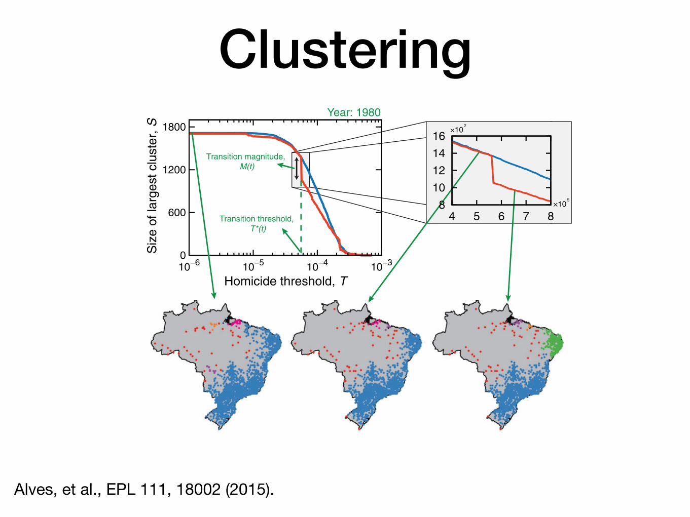
Fig. 3: (Color online) Formation of spatial cluster of cities and a percolation-like analysis. The plot shows the size of the largestcluster S (defined as the number of cities that belong to the cluster) as a function of the threshold T in the per capita homicides.The red line shows the results considering data from the year t = 1980 and the blue line shows the results after randomizingthe values of the per capita homicides hi(t) among the cities. For the original data (red line), we observe that S undergoesan abrupt change around a specific value of T = T ∗(t), followed by smaller subsequents abrupt changes. The inset shows amagnification of the region where this transition-like behavior occurs. The value of T ∗(t) is defined as the point at which thejump in S is maximum and we have further defined the transition magnitude M(t) as the size of this maximum jump (bothT ∗(t) and M(t) are illustrated in the plot). The three maps illustrate the clusters identified by the DBSCAN algorithm for thevalues of T indicated by the green arrows.

is a reaction term (leading us to a reaction-diffusion–likeequation). Another important aspect of our system is thediscrete and non-homogeneous spatial distribution of thecities, which may also play an important role on the spatialcorrelations. However, despite the importance of model-ing, we believe that this modeling question may deserve aseparated investigation.

The spatial correlations in hi(t) also provide anindication of the existence of spatial clusters of cities withsimilar values of per capita homicides. To address thisquestion, we study the formation of spatial cluster of citiesvia a percolation-like analysis [25,32,33]. Specifically, wedefine a homicide threshold T and select all cities for whichhi(t) ≥ T . For the set of cities satisfying this condition,we apply the density-based spatial clustering of applica-tions with noise algorithm (DBSCAN —as implementedin Python library Scikit-Learn [34]) for identifying pos-sible spatial clusters. This algorithm finds statisticallysignificant clusters and we have investigated the size ofthe largest cluster S (that is, the number of cities in thelargest cluster) as a function of the threshold T , as shownin fig. 3 (red line) for the year t = 1980. Analogously toa phase transition, S undergoes an abrupt change arounda specific value of T = T ∗(t), where the largest clusterstarts to be broken into smaller ones. A similar behaviorwas observed for obesity rates in the United States [25].In our case, the value of T ∗(t) is defined as the point atwhich the jump in S is maximum and we have further

defined the transition magnitude M(t) as the size of thismaximum jump. In this particular example, we have thatat T ∗(t = 1980) = 5.67× 10−5 the number of cities in thelargest cluster decreases by M(t = 1980) = 314. We fur-ther observe the existence of smaller subsequents abruptchanges in S, producing a staircase-like behavior in S. Inorder to confirm that this transition-like behavior is notonly related to the spatial location of the cities, we ran-domize the values of hi(t) among the cities and investigateagain the relationship between S and T . For the random-ized data, fig. 3 (blue line) shows that the size of the largestcluster continuously goes to zero as T increases. Thus, theintricate behavior of S vs. T observed for the original datacannot be directly related to the spatial distribution of theBrazilian cities.

We have applied the clustering analysis for all years inour dataset and a similar transition-like behavior is foundfor all of them, but with some evolutive features. Thecritical value T ∗(t) has increased over years with an ap-proximately linear rate of (0.10 ± 0.01) × 10−4 per capitahomicides per year, as shown in fig. 4(a). Naturally, thegrowth of T ∗(t) should be related to the overall increas-ing trend in the per capita homicides of Brazil (fig. 1). Inorder to account for this effect, we divide T ∗(t) by theoverall per capita homicides in Brazil h(t). Figure 4(b)shows that part of the evolutive behavior of T ∗(t) is ac-tually associated with h(t); however, a statistically signif-icant increasing trend is still observed for scaled threshold

18002-p4

Alves, et al., EPL 111, 18002 (2015).

Clustering

DRAFT10−2

10−1

100

0 10 20 30 40 5010−2

10−1

100

0 10 20 30 40 50

Caso

Bane

spa

(198

7)Fe

rrovia

Norte

-Sul

(198

7)CP

Ida

Corru

pção

(198

8)M

áfia

daPr

evid

ência

(199

1)Ca

soCo

llor(

1992

)An

ões

doO

rçam

ento

(199

3)Pa

ubra

sil(1

993)

Escâ

ndal

oda

Para

bólic

a(1

994)

Past

aro

sa(1

995)

Com

pra

devo

tos

para

are

elei

ção

(199

7)Es

când

alo

das

priva

tizaç

ões

(199

7)Fr

ango

gate

(199

7)Pr

ecat

ório

s(1

997)

Doss

iêCa

yman

(199

8)G

ram

pos

doBN

DES

(199

8)M

áfia

dos

fisca

is(1

998)

Caso

Mar

ka/F

onte

Cind

am(1

999)

Desv

ios

deVe

rbas

doTR

T-SP

(199

9)G

arot

inho

ea

turm

ado

Chuv

isco

(200

0)Su

dam

(200

1)Vi

olaç

ãodo

pain

eldo

Sena

do(2

001)

Bunk

erpe

tista

(200

2)Ca

soCe

lsoDa

niel

(200

2)Ca

soLu

nus

(200

2)CP

Ido

Bane

stad

o(2

003)

Ope

raçã

oAn

acon

da(2

003)

Banp

ará

(200

4)Ca

soG

Tech

(200

4)Ca

soW

aldo

miro

Dini

z(2

004)

Supe

rfatu

ram

ento

deob

ras

emSP

(200

4)Co

rrupç

ãono

sCo

rreio

s(2

005)

Dóla

res

nacu

eca

(200

5)Es

când

alo

doM

ensa

lão

(200

5)Re

públ

icade

Ribe

irão

(200

5)Va

lerio

duto

min

eiro

(200

5)Al

opra

dos

(200

6)Es

când

alo

dos

sang

uess

ugas

(200

6)Q

uebr

ade

sigilo

doca

seiro

Fran

ceni

ldo

(200

6)Ch

eque

daG

ol(2

007)

Rena

ngat

eCa

sodo

lara

njal

alag

oano

(200

7)Re

nang

ate

Caso

Môn

icaVe

loso

(200

7)Re

nang

ate

Caso

Schi

ncar

iol(

2007

)Re

nang

ate

Gol

peno

INSS

(200

7)Ca

rtões

corp

orat

ivos

(200

8)Ca

soSa

tiagr

aha

(200

8)Do

ssiê

cont

raFH

Ce

Ruth

Card

oso

(200

8)Pa

ulin

hoda

Forç

ae

oBN

DES

(200

8)At

osSe

cret

os(2

009)

Caso

Lina

Viei

ra(2

009) M

ensa

lão

doDE

M(2

009)

Banc

oop

(201

0)Ca

soEr

enice

(201

0)O

sno

vos

alop

rado

s(2

010)

Escâ

ndal

oem

Cida

des

(201

1)Es

când

alo

naAg

ricul

tura

(201

1)Es

când

alo

noEs

porte

(201

1)Es

când

alo

nos

Tran

spor

tes

(201

1)Es

când

alo

noTr

abal

ho(2

011)

Escâ

ndal

ono

Turis

mo

(201

1)Ca

soCa

choe

ira(2

012)

Escâ

ndal

ona

Pesc

a(2

012)

Ope

raçã

oPo

rtoSe

guro

(201

2)M

áfia

doIS

S(2

013)

Ope

raçã

oLa

vaJa

to(2

014)

Petro

lão

(201

4)

0

10

20

30

40

−0.20.00.20.40.60.81.0

0 2 4 6 8 10

−0.20.00.20.40.60.81.0

0 2 4 6 8 100

15

30

45

60

75

1986 1992 1998 2004 2010 20160

15

30

45

60

75

1986 1992 1998 2004 2010 2016

Num

ber o

f peo

ple

Cum

ulat

ive d

istrib

utio

n

Number of people Year Lag (years)

Num

ber o

f peo

ple

Auto

corre

latio

n

Corruption case

DCB

A

7.51 ± 0.03

1.2 ± 0.4

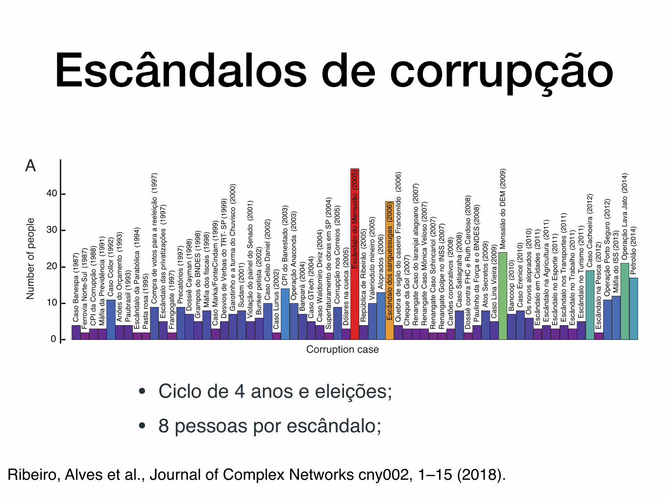
Fig. 1. Demography and evolving behavior of corruption scandals in Brazil. A) The number of people involved in each corruption scandal in chronological order (from 1987 to2014). B) Cumulative probability distribution (on a log-linear scale) of the number of people involved in each corruption scandal (red circles). The dashed line is a maximumlikelihood fit of the exponential distribution, where the characteristic number of people is 7.51 ± 0.03. The Cramér-von Mises test cannot reject the exponential distributionhypothesis (p-value = 0.05). C) Time series of the number of people involved in corruption scandals by year (red circles). The dashed line is a linear regression fit, indicating asignificant increasing trend of 1.2 ± 0.4 people per year (t-statistic = 3.11, p-value = 0.0049). D) Autocorrelation function of the time series of the yearly number of peopleinvolved in scandals (red circles). The shaded area represents the 95% confidence band for a random process. It is worth noting that the correlation oscillates while decayingwith an approximated four-year period, the same period in which the general elections take place in Brazil.

in each scandal, finding out that it can be well describedby an exponential distribution with a characteristic numberof involved around eight people (Fig. 1B). A more rigorousanalysis with the Cramér-von Mises test confirms that theexponential hypothesis cannot be rejected from our data (p-value = 0.05). This exponential distribution confirms thatpeople usually act in small groups when involved in corruptionprocesses, suggesting that large-scale corruption processes arenot easy to manage and that people try to maximize theconcealment of their crimes.

Another interesting question is related to how the number ofpeople involved in these scandals has evolved over the years. InFig. 1C we show the aggregated number of people involved incorruption cases by year. Despite the fluctuations, we observea slightly increasing tendency in this number, which can bequantified through linear regression. By fitting a linear model,we find a small but statistically significant increasing trendof 1.2 ± 0.4 people per year (p-value = 0.0049). We also askif this time series has some degree of memory by estimatingits autocorrelation function. Results of Fig. 1D show thatthe correlation function decays fast with the lag-time, andno significant correlation is observed for time series elementsspaced by two years. However, we further note a harmonic-likebehavior in which the correlation appears to oscillate whiledecaying. In spite of the small length of this time series, weobserve two local maxima in the correlation function that areoutside the 95% confidence region for a completely random

process: the first between 3 and 4 years and another between8 and 9 years. This result indicates that the yearly time seriesof people involved in scandals has a periodic component withan approximated four-year period, matching the period inwhich the Brazilian elections take place. Again, this behaviorshould be considered much more carefully due to the smalllength of the time series. Also, this coincidence does notprove any causal relationship between elections and corruptionprocesses, but it is easy to speculate about this parallelism.Several corruption scandals are associated with politicianshaving exercised improper influence in exchange for undueeconomic advantages, which are often employed for supportingpolitical parties or political campaigns. Thus, an increase incorrupt activities during election campaigns may be one ofthe reasons underlying this coincidence.

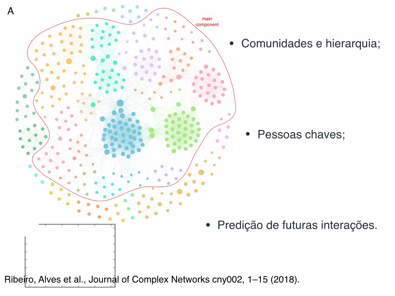
Network Representation of Corruption Scandals. In order tostudy how people involved in these scandals are related, wehave built a complex network where nodes are people listed inscandals, and the ties indicate that two people were involved inthe same corruption scandal. This is a time-varying network,in the sense that it grows every year with the discovery of newcorruption cases. However, we first address static properties ofthis network by considering all corruption scandals together,that is, the latest available stage of the time-varying network.Figure 2A shows a visualization of this network that has404 nodes and 3549 edges. This network is composed of 14

Ribeiro et al. PNAS | September 27, 2017 | vol. XXX | no. XX | 3

Ribeiro, Alves et al., Journal of Complex Networks cny002, 1–15 (2018).

Escândalos de corrupção

• Ciclo de 4 anos e eleições;

• 8 pessoas por escândalo;

A

B

maincomponent

−3−2−1

01234

0.0 0.2 0.4 0.6 0.8 1.0

−3−2−1

01234

0.0 0.2 0.4 0.6 0.8 1.0

With

in-m

odul

e de

gree

, Z

Participation coeficient, P

R7R6R5

R1 R2 R3 R4

• Predição de futuras interações.

• Pessoas chaves;

Ribeiro, Alves et al., Journal of Complex Networks cny002, 1–15 (2018).

• Comunidades e hierarquia;

Obrigado@lgaalves

[email protected]

@lgaalves

https://lgaalves.github.io/

Física estatística do crime: leis de escala...

Documents

Transcript of Física estatística do crime: leis de escala...