falcON

a Cartesian FMM for the low-accuracy regime

College Park, 28th April 2004

Journal of Computational Physics, 179, 27-42 (2002)

Walter Dehnen (Leicester)walter.dehnen@astro.le.ac.uk

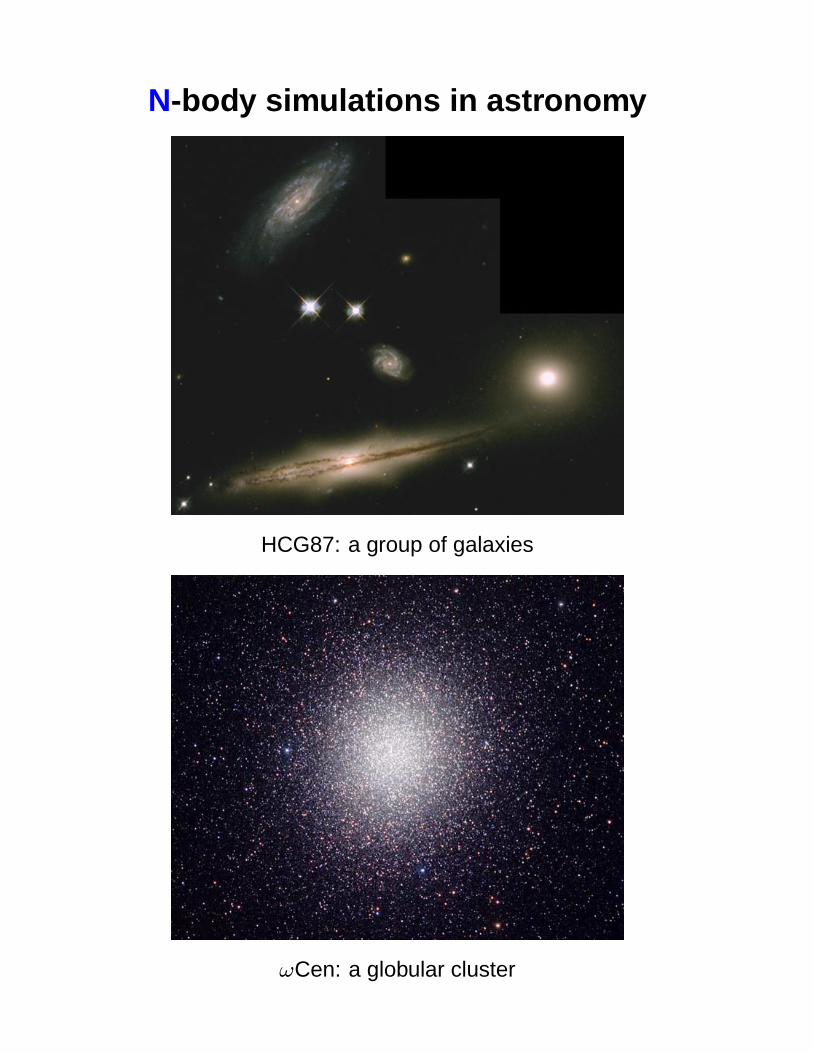
N-body simulations in astronomy

HCG87: a group of galaxies

ωCen: a globular cluster

properties of stellar systems

� simple physics: Newtonian gravity� very inhomogeneous⇒ large dynamic range

� dynamically young (tdyn ' Myr–Gyr)� well approximated as ensembles of point masses⇒ well described as Hamiltonian systems

(⇒ need symplectic time integration)

H =N∑

i=1

mi

2

v2i −

∑j 6=i

G mj

|xi − xj|

, vi = xi =pi

mi

with N ' 105−20

� equation of motion in continuum (mean-field) limit:

0 =df

dt=

∂f

∂t+

∂f

∂x· v −

∂f

∂v·∂Φ

∂x

collisionless Boltzmann equation (CBE)

� f(x, v, t): distribution function (density in phase space)

� Φ(x) : mean-field gravitational potential

both are related via the Poisson equation :

∇2Φ(x) = 4πG∫d3v f(x, v, t)

two-body relaxation

How good is the continuum description?

� stellar encounters deflect trajectories⇒ stellar orbits get randomized⇒ Maxwellian velocity distribution

� two-body relaxation time :

trelax ' 0.1N

logNtdyn

1 collision-dominated stellar dynamics

� trelax ∼< age of system

⇒ continuum limit not applicable⇒ must simulate Hamiltonian directly:

� force computation is O(N2)

⇒ computational effort limits N ∼< 105

� close encounters are important⇒ time integration becomes tedious

2 collisionless stellar dynamics

� trelax � age of system

⇒ continuum limit applicable⇒ solve CBE & Poisson equation

‘collisionless’ N-body simulations

How to solve the CBE?

0 =df

dt=

∂f

∂t+

∂f

∂x· v −

∂f

∂v·∂Φ

∂x

� f is 6D & very inhomogeneous⇒ (Eulerian) grid methods are useless⇒ Lagrangian method (‘method of characteristics’):

� sample N trajectories {µi, xi, vi} from f(x, v, t = 0)

� solve equations of motion xi = −∇Φ(xi, t)

� CBE: µi = const along trajectories

⇒ f(x, v, t) is represented by {µi, xi(t), vi(t)}⇒ f is unknown

⇒ moments of f can be estimated

⇒ N � N is numerical parameter

⇒ artificial two-body relaxation

How to solve the Poisson equation?

∇2Φ(x) = 4πG∫d3v f(x, v, t)

1 grid techniques (FFT, multigrid):� fast: O(ngrid logngrid)

� periodic (⇒ cosmology)� problem: inhomogeneity (but: adaptive multigrid)

2 basic functions (using Ylm):� fast: O(Nnbasis)

� problems: central singularity, spherical symmetry

3 Greens-function approach:

Φ(x, t) = −G∫d3x′ d3v

f(x′, v, t)

|x− x′|

� general & adaptive� problem: f is unkown⇒ estimate (ε: softening length )

Φ(xi, t) ≈ −∑i6=j

G µj√[xi − xj(t)]

2 + ε2

force softening to� optimize force estimate (since f is unknown)� suppress (unphysically) close encounters⇒ force-estimation error (unavoidable)

true gravity of Hernquist model

estimation error with N = 106

computing the forces

� Greens-function approach → Hamiltonian:

H =N∑

i=1

µi

2

v2i −

∑j 6=i

G µj√|xi − xj|2 + ε2

� how to evaluate Φ & ∇Φ?� can tolerate approximation error � estimation error⇒ use approximative methods

1 direct summation (not approximative):� slow: O(N2) (but: GRAPE)� (unnecessarily) accurate� used in collisional N-body codes

2 Barnes & Hut (1986) tree code :� use hierarchical tree (usually: oct-tree) ⇒ fully adaptive� fast(er): O(N logN)

� most common method in astrophysics� violates Newton’s 3rd law⇒ total momentun not conserved

3 traditional fast multipole method (FMM):� use hierarchy of cartesian grids ⇒ not fully adaptive� compute gravity via spherical multipoles & complex Ylm

⇒ numerics complicated & cumbersome� formally O(N), but

slower than tree code (for astrophyiscal applications,see Capuzzo-Colcetta & Miochi, 1998, JCP, 143, 29)

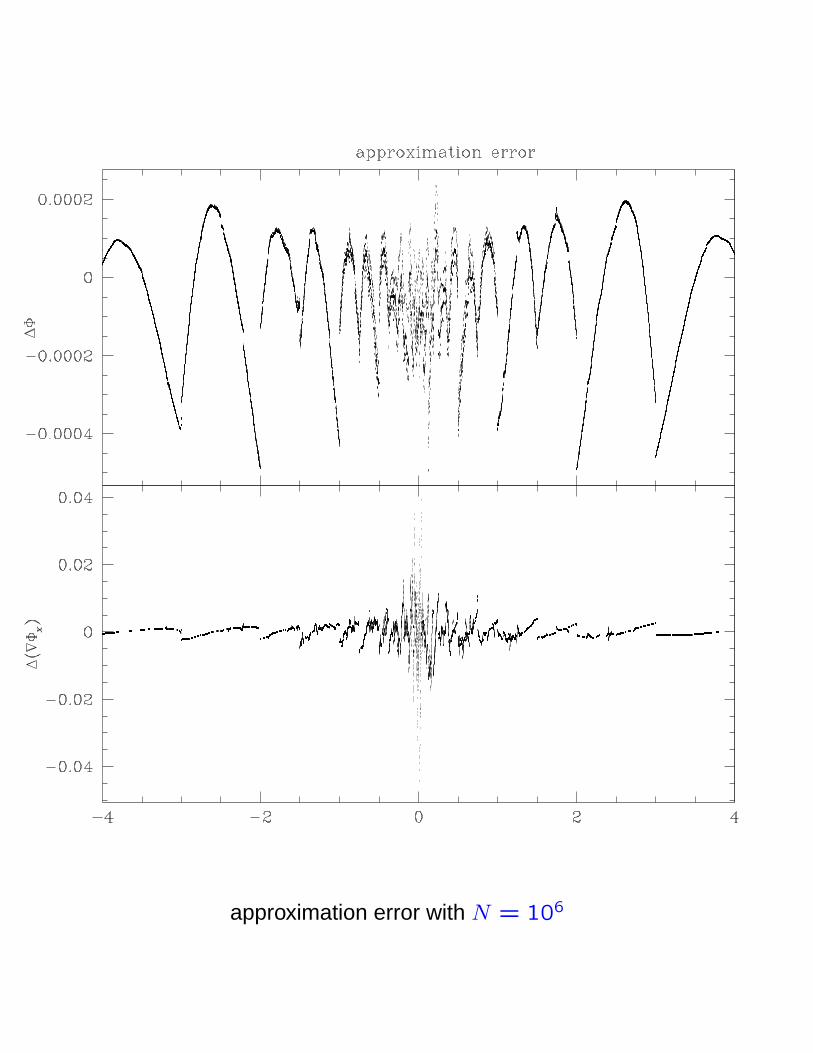
approximation error with N = 106

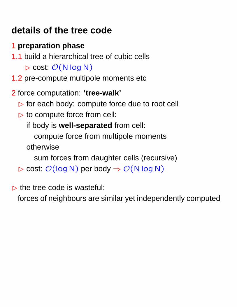
details of the tree code

1 preparation phase1.1 build a hierarchical tree of cubic cells

� cost: O(N logN)

1.2 pre-compute multipole moments etc

2 force computation: ‘tree-walk’� for each body: compute force due to root cell� to compute force from cell:

if body is well-separated from cell:compute force from multipole moments

otherwisesum forces from daughter cells (recursive)

� cost: O(logN) per body ⇒O(N logN)

� the tree code is wasteful:forces of neighbours are similar yet independently computed

details of the FMM

here I describe traditional Greengard & Rokhlin (1987) FMM

1 preparation phase1.1 build a hierarchy of cartesian grids1.2 pre-compute multipole moments etc (upward pass )

2 force computation

2.1 interactionson each grid level:� perform ‘intermediate-field’ interactions:

compute & accumulate multipoles of gravity field

2.2 downward pass� pass field-multipoles down the hierarchy� compute forces on finest grid

� theoretical O(N) not demonstrated in practice� not competetive with tree code in low-accuracy regime

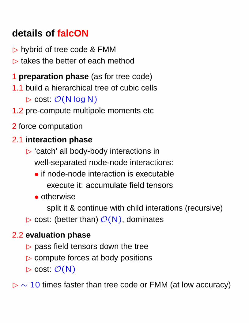
details of falcON

� hybrid of tree code & FMM� takes the better of each method

1 preparation phase (as for tree code)1.1 build a hierarchical tree of cubic cells

� cost: O(N logN)

1.2 pre-compute multipole moments etc

2 force computation

2.1 interaction phase� ‘catch’ all body-body interactions in

well-separated node-node interactions:• if node-node interaction is executable

execute it: accumulate field tensors• otherwise

split it & continue with child interations (recursive)� cost: (better than) O(N), dominates

2.2 evaluation phase� pass field tensors down the tree� compute forces at body positions� cost: O(N)

� ∼ 10 times faster than tree code or FMM (at low accuracy)

numerics of falcON

Wanted:

Φ(xi) = −∑j 6=i

µj g(xi − yj),

Taylor expand g about R = x0 − y0

g(x− y) =p∑

n=0

1

n!(x− y−R)(n)�∇(n)g(R) + Rp(g),

Insert & sum over source cell B

ΦB→A(x)=−p∑

m=0

1

m!(x− x0)

(m) � Cm,p + Rp(ΦB→A)

Cm,p =p−m∑n=0

(−1)n

n!∇(n+m)g(R)�Mn

B,

MnB =

∑yi∈B

µi (yi − y0)(n).

(Warren & Salmon 1995: Comp. Phys. Comm, 87, 266)∑m : evaluation of gravity, represented by the field

tensors Cm,p, at position x∑n : interaction between source cell B, represented

by the multipoles MnB, and the sink cell A.

Difference to tree code:� expansion in x (tree code: x ≡ x0)� mutuality of inter actions

gravity between well-seperated nodes

two well-separated cells

If |R| > rA,crit + rB,crit with rcrit = rmax/θ,

⇒ |x−y−R|<θ|R| ∀ x∈A, y∈B & Taylor series converges

force error of individual interaction:

|∇Rp(ΦB→A)| ≤(p + 1)θp

(1− θ)2MB

R2

∝θp+2

(1− θ)2rd−2B,max ∝

θp+2

(1− θ)2MB

(d−2)/d

� standard tree-code & FMM practice: θ = const⇒ relative error controlled⇒ absolute error increases with MB⇒ total error dominated by few interactions with large cells

⇒ better:� balance absolute individual errors by θ = θ(M) with

θp+2

(1− θ)2=

θp+2min

(1− θmin)2

(M

Mtot

)(2−d)/d

⇒ reduce total error

accuracy vs. CPU time

mean (dashed) and 99 percentile (solid) relative force error

ε ≡ |aapprox − aexact|/aexact,

versus the CPU time (Pentium III/933Mhz in 2001) for a galaxy (left) and a

group f galaxies (right), sampled with (total) N = 104 (top), N = 105 (mid-

dle), or N = 106 (bottom). We used either θ = const (open triangles)

or θ = θ(M) (solid squares). The symbols along each curve correspond,

from left to right, to values for θ or θmin of 0.2, 0.3, 0.4, 0.5, 0.6, 0.7, and

0.8.

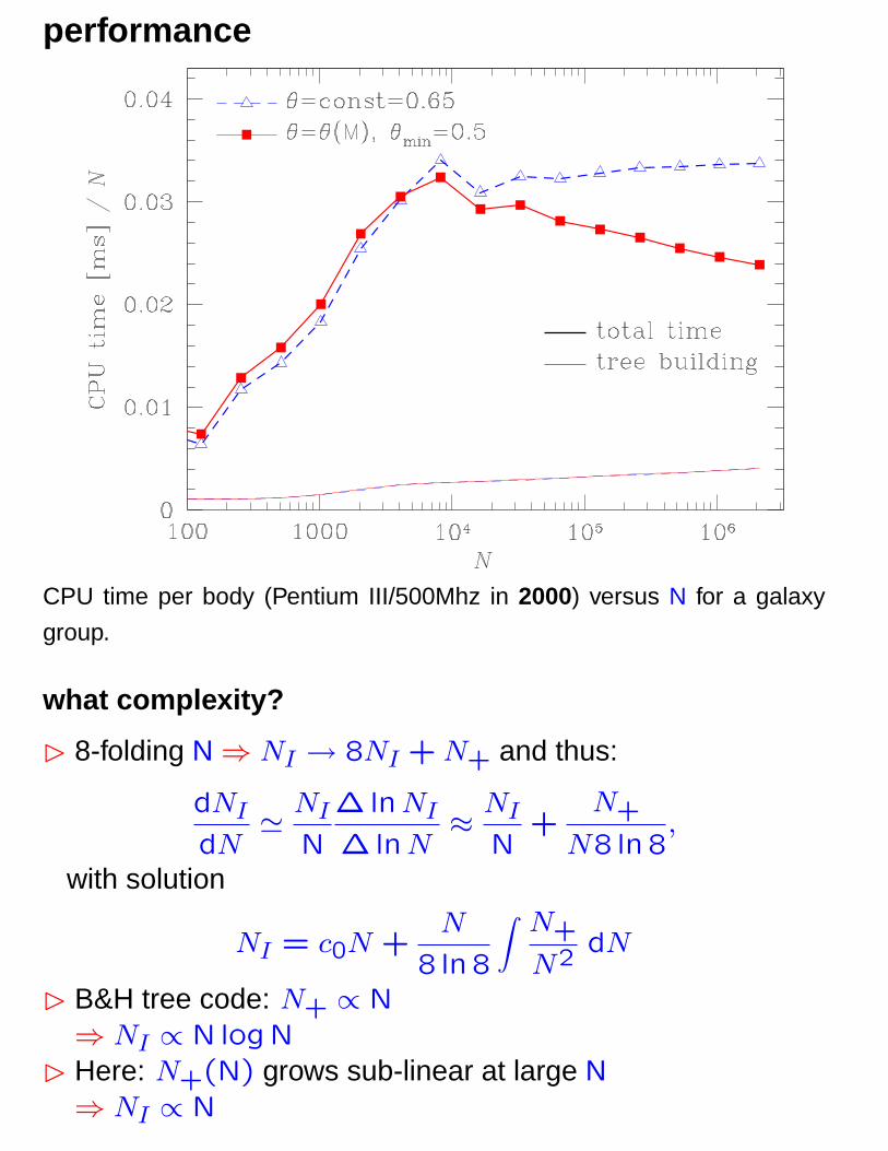
performance

CPU time per body (Pentium III/500Mhz in 2000) versus N for a galaxy

group.

what complexity?

� 8-folding N ⇒ NI → 8NI + N+ and thus:

dNI

dN'

NI

N

∆lnNI

∆lnN≈

NI

N+

N+

N8 ln 8,

with solution

NI = c0N +N

8 ln 8

∫ N+

N2dN

� B&H tree code: N+ ∝ N⇒ NI ∝ N logN

� Here: N+(N) grows sub-linear at large N⇒ NI ∝ N

comparison with other methodsused in astrophysics

CPU time per body (2001) versus N for various techniques. Note that

there are differences in the hard- & software, stellar system, and accuracy

requirements.

by 2003/2004: falcON is ∼ 3 times faster, but GRAPE-5 tree not.

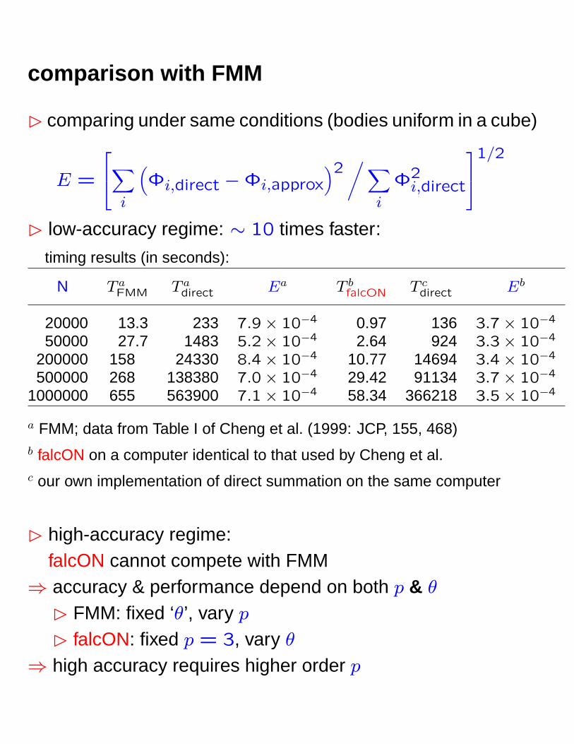
comparison with FMM

� comparing under same conditions (bodies uniform in a cube)

E =

∑i

(Φi,direct −Φi,approx

)2/∑i

Φ2i,direct

1/2

� low-accuracy regime: ∼ 10 times faster:

timing results (in seconds):

N T aFMM T a

direct Ea T bfalcON T c

direct Eb

20000 13.3 233 7.9× 10−4 0.97 136 3.7× 10−4

50000 27.7 1483 5.2× 10−4 2.64 924 3.3× 10−4

200000 158 24330 8.4× 10−4 10.77 14694 3.4× 10−4

500000 268 138380 7.0× 10−4 29.42 91134 3.7× 10−4

1000000 655 563900 7.1× 10−4 58.34 366218 3.5× 10−4

a FMM; data from Table I of Cheng et al. (1999: JCP, 155, 468)b falcON on a computer identical to that used by Cheng et al.c our own implementation of direct summation on the same computer

� high-accuracy regime:falcON cannot compete with FMM

⇒ accuracy & performance depend on both p & θ

� FMM: fixed ‘θ’, vary p

� falcON: fixed p = 3, vary θ

⇒ high accuracy requires higher order p

summary

� falcON = hybrid of tree code & FMM

� new features:• explicitly exploits mutuality of gravity⇒ reduces computational effort⇒ requires novel tree-walking algorithm⇒ conservation of Newton’s 3rd law

• mass-dependent θ

⇒ error balancing⇒ reduces cost to better than O(N)

� ∼ 10 times faster than tree code or FMM

� publicly available

more dogmas

� balance errors⇒ reduce effort at given accuracy

� keep algorithm as simple as possible &as complicated as necessary

⇒ high-order may be unnecessary

� write efficient code⇒ avoid cache misses⇒ data structure design

⇒ write generic code⇒ do not rely too much on compliler optimization⇒ template metaprogramming