EXPERIMENTAL STUDY OF FLOW INDUCED TENSION...
148
EXPERIMENTAL STUDY OF DRAG FROM A FLUTTERING FLAG By ADAM MARTIN Bachelor of Science Oklahoma State University Stillwater, Oklahoma 2003 Submitted to the Faculty of the Graduate College of the Oklahoma State University in partial fulfillment of the requirements for the Degree of MASTER OF SCIENCE May, 2006
Transcript of EXPERIMENTAL STUDY OF FLOW INDUCED TENSION...

EXPERIMENTAL STUDY OF DRAG FROM A
FLUTTERING FLAG
By
ADAM MARTIN
Bachelor of Science
Oklahoma State University
Stillwater, Oklahoma
2003
Submitted to the Faculty of the Graduate College of the
Oklahoma State University in partial fulfillment of
the requirements for the Degree of
MASTER OF SCIENCE May, 2006
ii
EXPERIMENTAL STUDY OF DRAG FROM A
FLUTTERING FLAG
Thesis Approved:
Dr. Peter M. Moretti Thesis Adviser
Dr. Andrew S. Arena
Dr. Frank W. Chambers
Dr. A. Gordon Emslie Dean of the Graduate College

iii
ACKNOWLEDGEMENTS
I would like to express my most sincere gratitude to my advisor, Dr. Peter
Moretti, for his excellent guidance, consistent encouragement, and dedication to teaching
and research. For their time and helpful comments, I am grateful for my committee
members: Dr. F.W. Chambers and Dr. A.S Arena.
I would also like to express my appreciation to Dr. J.K. Good and Dr. F.W.
Chambers for their generosity in sharing test equipment for experimental measurements;
to Mr. Ron Markum for teaching me to weld, to Mr. Jerry Dale for suggestions during
set-up construction, and to Nic Moffitt for his helpful conversations and wind tunnel
orientation. Furthermore, I would like to thank Dr. Young Chang for his encouragement
during the course of this study.
My gratitude extends to my parents, whose support and encouragement are
priceless. Above all, I thank my Heavenly Father for establishing the work of my hands.

iv
TABLE OF CONTENTS
Chapter Page
I. INTRODUCTION ...................................................................................................1
1.1 Background.....................................................................................................1 1.2 Objectives and Scope of Study .......................................................................2 1.3 Methods of Study............................................................................................3
II. LITERATURE REVIEW ........................................................................................5
2.1 Flutter phenomena ..........................................................................................5 Fundamental Trends.................................................................................... 7 Flutter Overview ......................................................................................... 9 Drag Approximations................................................................................ 11
III. THEORIES ............................................................................................................16
3.1 Fundamentals of Drag and Lift .....................................................................16 Classical Drag of a cylinder in a fluid stream........................................... 16 Classical Lift ............................................................................................. 23
3.2 Stiff Vane Drag in a Fluid Stream ................................................................24 Laminar Boundary Layer.......................................................................... 25 Turbulent Boundary Layer........................................................................ 28
3.3 Flexible Vane Drag in a Fluid Stream ..........................................................34
IV. EXPERIMENTAL STUDY...................................................................................36
4.1 Experimental Setup.......................................................................................36 Wind Tunnel Test Section ........................................................................ 36 Attachment Pole........................................................................................ 39 Drag/Lift Measurements ........................................................................... 41 Pressure Measurements............................................................................. 43 Frequency Measurements ......................................................................... 47 Mode Shape Measurements ...................................................................... 52
4.2 Experimental Procedure................................................................................56 4.3 Estimation of the Uncertainty of Drag Force................................................61 4.4 Experimental Results ....................................................................................65
Light-Weight Flexible Sheet μ =0.704 ..................................................... 65 Semi-Rigid Cooking Board μ =1.74 ......................................................... 68 Heavy-Weight Flexible Sheet μ =1.88 ..................................................... 70 Overall Comparison .................................................................................. 86

v
Conservation of Momentum Drag Analysis ............................................. 92
V. CONCLUSIONS..................................................................................................103
Drag Overview........................................................................................ 103 Wave Characteristics .............................................................................. 105
REFERENCES ................................................................................................................107
APPENDICES .................................................................................................................109
APPENDIX A—WIND TUNNEL TEST SECTION DRAWINGS...................110 APPENDIX B—MATLAB VELOCITY CONTOUR M-FILE..........................114 APPENDIX C—STEPPING MOTOR WIRING SCHEMATIC........................115 APPENDIX D—STEPPING MOTOR DRIVER CIRCUIT...............................117 APPENDIX E—LABVIEW PITOT TRAVERSE MOTOR CONTROL...........118 APPENDIX F—PITOT TUBE PRESSURE UNCERTAINTY..........................119 APPENDIX G—MATLAB CROSS-POWER-SPECTRUM M-FILE ...............121 APPENDIX H—LABVIEW FFT FRONT PANEL POWER SPECTRUM VI. 125 APPENDIX I—EXCEL SHEET AIR PROPERTY CALCULATOR................126 APPENDIX J—EXCEL AIR PROPERTY CALCULATOR FORMULAS ......127 APPENDIX K—FREE-STREAM PRESSURE PROFILES ..............................129

vi
LIST OF FIGURES
Figure Page
1. Flexible sheet diagram illustrating span and chord length.......................................6
2. Diagram of a fluttering specimen ..........................................................................10
3. Drag Coefficient vs. fineness ratio as presented by Fairthorne (1930).................12
4. Relative magnitude and distribution of dynamically induced tension vs. skin friction (viscous) drag. ...........................................................................................15
5. Cross-section of a cylinder in a fluid stream .........................................................18
6. Theoretical and experimental profile of drag vs. velocity for a circular cylinder ( )1.0DC = ..............................................................................................................22
7. Experimental accuracy with a known drag case ....................................................23
8. Classical airfoil diagram of forces .........................................................................24
9. Comparison of laminar and turbulent boundary layer drag for a stiff panel. ........29
10. Combined Drag force of pole and stiff vane attachment .......................................30
11. Specimen dimensions for all experimental drag tests............................................31
12. Stiff panel specimen (aluminum) with no air supply.............................................31
13. Pole drag dominating stiff panel drag....................................................................32
14. Proof superposition of drag cases is inaccurate .....................................................33
15. Diagram of forces on a flexile web........................................................................35
16. Wind tunnel test section illustration with specimen and pitot tube probe. ............37
17. Wind tunnel experimental set-up ...........................................................................38
18. Attachment pole .....................................................................................................40
19. Flag pole with flexible specimen µ=1.88...............................................................40
20. Coupled drag and lift transducers ..........................................................................41
21. Lift and Drag Measurement on a Fluttering Flag ..................................................42
22. Schematic of a pitot static tube. .............................................................................43
vii
23. Pitot static tube traverse .........................................................................................45
24. Free stream velocity profile using bi-directional traverse. ....................................46
25. Vibrometer Set-up..................................................................................................48
26. Cross spectrum test confirming 90° phase shift of sine and cosine function. .......50
27. Cross FFT frequency and phase information for a flexible sheet at 3.43 m/s. ......51
28. High speed camera set-up ......................................................................................53
29. Amplitude measurement from high speed photo data ...........................................54
30. Heavy sheet deflection modes 8.41 m/s (μ=1.88) .................................................55
31. Experimental set-up ...............................................................................................57
32. Drag Calibration Set-up .........................................................................................59
33. Drag calibration linear curve fit μ=1.88 ................................................................62
34. Drag results for heavy sheet μ=1.88 ......................................................................63
35. Sudden flutter onset and fall-off for a flexible fabric with very low stiffness.......66
36. Experimental drag comparison (μ=0.704) with empirical prediction Fairthorne (1930).....................................................................................................................67
37. Semi-Rigid Cooking Board....................................................................................68
38. Fundamental frequency and traveling phase angle (cutting board μ=1.17) ..........69
39. Cooking board drag results ....................................................................................70
40. Schematic of the wind tunnel and test specimen ...................................................71
41. Velocity wake of fluttering specimen μ=1.88 .......................................................71
42. Increasing flutter frequency and phase with velocity (μ=1.88) .............................72
43. Traveling waves from high speed images separated by two complete cycles.......74
44. High speed modal data at 8.41 m/s (μ=1.88).........................................................76
45. Change in inflection amplitude with wavelength over 2 periods. .........................77
46. Experimental drag data μ=1.88..............................................................................78
47. Example amplitude measurement from image data...............................................80
48. Amplitude results from high speed camera pixel correlation ................................81
49. Experimental comparison of drag with theory [Thoma / Moretti].........................82
50. Least squares curve fit of experimental drag data .................................................83
51. Component of dynamically induced drag μ=1.88 .................................................84
viii
52. Experimental comparison of drag with empirical prediction [Fairthorne (1930)]85
53. Picture of three materials tested.............................................................................87
54. Effect of flutter frequency with material property.................................................88
55. Effect of traveling speed with material stiffness....................................................89
56. Frequency and phase relationship (cooking board and flexible sheet) ..................90
57. Experimental drag data ..........................................................................................91
58. Comparison of net drag with dynamically induced drag .......................................92
59. Momentum principle diagram of forces ................................................................94
60. Pressure drop as a result of fluid boundary layer along tunnel walls ....................96
61. Velocity wake profile at 8.68 m/s. .........................................................................97
62. Horizontal velocity profile at 8.68 m/s ..................................................................97
63. Vertical velocity profile at 8.68 m/s ......................................................................98
64. Pressure profile (contoured and discrete) at 8.68 m/s............................................99
65. Free stream pressure profile (grid data) 8.68 m/s ................................................100
66. Theoretical momentum drag analysis with experimental results.........................101
67. Pressure profile in the wake of a flexible cutting board at 8.89 m/s....................102
68. Closed form approximations with experimental data ..........................................104
69. Amplitude shape approximation for measurements at the leech .........................106
70. “Ground to Excite” schematic of our 4-phase stepper sequence. ........................115
71. Vertical pressure distribution...............................................................................135
72. Effect of vertical pressure profile from taping pitot slot......................................136

ix
NOMENCLATURE
A Characteristic Area normal to flow field
C Chord length
DC Drag coefficient
D Cylinder diameter
DF Drag force
LF Lift force
DpF Pressure drag force (form drag)
DvF Viscous drag force (skin friction)
Hzf Flutter frequency (hertz)
g Acceleration due to gravity
L Stiff panel length (chord length)
m Mass per unit area
m Mass flow rate
atmp Atmospheric pressure
1p Free-stream pressure upstream of disturbance
sp Stagnation pressure where fluid velocity 0V =
pΔ Pressure difference ( )1 sp p−
Q Volumetric flow rate
R Universal gas constant for air

x
DRe Reynolds number based on cylinder diameter, ( )0 /U D μ ρ
LRe Reynolds number based on stiff panel chord length, ( )0 /U L μ ρ
S Span of web (flag width)
roomT Room temperature
0U Free stream fluid velocity
v Local fluid velocity
x Direction parallel to free-stream air velocity
y Direction normal to free-stream air velocity
μ Dynamic viscosity of air
,mr μ Mass ratio, air
mmrC
μρ
= =
airρ Density of air
1
CHAPTER I
INTRODUCTION
1.1 Background
Webs are defined as continuous, strip-formed, flexible materials such as paper,
metal foils and polymer films. In many web-handling applications it is common that a
web will be coated on one side (as in photography film or tape) such that when
processing the web, it is necessary to have no mechanical contact on the coated side of
the web during processing. One way to process a web in such a case, is with air bars.
The web is “floated” and moved along its web line at high speeds. This air-web
interacting creates many instability problems when transporting the web quickly through
its production line. With increasing operation speed, the speed of the airflow around the
web during processing also increases, and flutter occurs. A web can oscillate
uncontrollably when one or several parameters dealing with tension, turbulence, and web
non-uniformity are not met. Such an oscillation can become violent very quickly, often
tearing the web. This occurrence is catastrophic in the production industry, where an
entire web line will be shut down, cleaned, and restrung, resulting in significant “down”
time and financial loss.
Another common instability problem that occurs in high-speed printing operations
is sheet flutter, sometimes called “flag flutter”. Unlike web flutter, sheet flutter has a
2
short chord length, and is unsupported at one or both ends. In printing presses, when a
continuous web is cut into sheets (leaflets), moments of flutter instability are common
when the sheet is cut or during its non-contact (floated) travel to the stack, where
undesirable touchdown or jamming can occur. With typical newsprint machines running
as fast as 1800 m/min (30 m/s), unsightly flutter can cause huge pileups and substantial
production downtime. Watanabe (2002) provides detailed diagrams and explanations of
the printing process. Through the efforts of many researchers studying such flutter
phenomena, it hoped that critical operational parameters can be applied in industry from
what work has been done to understand and predict the negative flutter phenomenon.
1.2 Objectives and Scope of Study
Flutter instability has been studied in varying degrees of detail and emphasis.
Some studies have emphasized material dimensions, others on various material
properties, yet others on mode deflections. Most studies have been conducted in a
manner that study a very wide range of materials, dimensions, and operating conditions
in generalized detail to understand the physics, and/or to look for underlying trends.
Additionally, it appears that most studies have been conducted in small-scale wind
tunnels using small specimen samples. This experiment is likely the most elaborate to
date for a single test specimen, with a dedicated wind tunnel and measurement system
designed for the purpose of flutter experimentation. After preliminary trial and error
wind tunnel runs, a suitable specimen was found that would flutter consistently in two
dimensions, (no irregular 3-D deflection modes) over a wide wind tunnel velocity range.
This study focuses its attention on this successful specimen, and seeks to understand the

3
induced component of drag during steady flutter oscillations. Additionally the
characteristics of the flutter mode (frequency, phase, amplitude, and wavelength) are
important and have only been partially uncovered by other researchers. The main
objectives of this study are listed as follows:
(1) To experimentally verify the components of drag for a fluttering specimen.
(2) To relate characteristic mode properties (frequency, phase, amplitude, and
wavelength) and investigate their role with changing material stiffness.
(3) To qualitatively describe the physics of flutter by relating experimental results
and compare closed form theoretical models with experimental results.
This study does not attempt to compare a wide range of fluttering specimens, but to
accurately and completely study one consistent flutter case. Because this is an
experimental study, detailed theoretical work will not be discussed, however it should be
noted that most theoretical analysis to date has been done via extensive numerical
simulation. To this avail, few closed form approximations and/or experimental
correlations have been presented.
1.3 Methods of Study
To understand the effects of dynamically induced tension in a fluttering specimen
we can build off classical studies of drag. First we can mathematically quantify the drag
force on our attachment pole, “flag pole”, by solving the classical drag problem of a
cylinder subject to cross flow; perpendicular to the pole’s axial axis. This first test
primarily serves as a check to validate the accuracy of our measurement system with that
of a classical solution. Secondly, we can add a rigid vane (a stiff panel incapable of

4
flutter) to the attachment pole and measure the drag force at the pole to quantify the
combined effects of pressure drag (from the flagpole) and minute viscous drag (skin
friction from the rigid panel). By studying the effects of a rigid panel attached to the
flagpole (an experimental constant for all flutter tests) the effect of the combined pressure
(form) drag can be accessed. Furthermore, the dominance of pressure drag over viscous
drag can be confirmed. With a baseline measurement of the “rigid” panel, we can attach
a flexible web material (flag) with the same dimensions and note the change of drag. The
difference between the drag of the flag specimen, to that of the rigid panel is the
dynamically induced drag.
5
CHAPTER II
LITERATURE REVIEW
The literature relevant to the present study comes from various authors presenting
analytical and experimental results of the “flag flutter” phenomenon. This topic has been
studied in detail, but still the sometimes random phenomena of flutter poses many
unknowns. Over the years however, many researcher have confirmed and reported some
of the same fundamental observation and experimental trends. This chapter will present
some of the results of past and help provide an underlying understanding of flutter and
the drag it creates.
2.1 Flutter phenomena
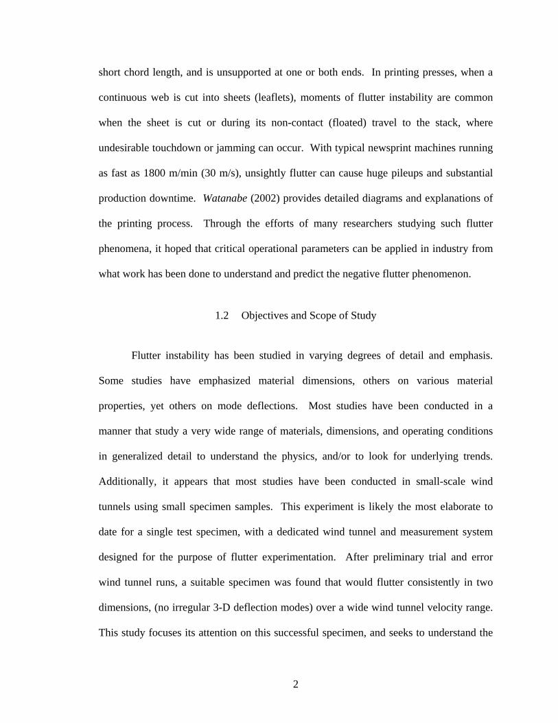
Flutter phenomena changes with varying specimen dimensions and “aspect
ratios”. The widely accepted (non-dimensional) definition of a specimen’s relative span
and chord dimension is called the “aspect ratio”.
Aspect Ratio Span SChord C
= =
This definition is made clear in Figure 1, where the aspect ratio is shown among
other terminology that will be used throughout this paper.
6
FlexibleSheet
Chord
Span
C
S
LeechLuff
AttachmentPole
Figure 1. Flexible sheet diagram illustrating span and chord length
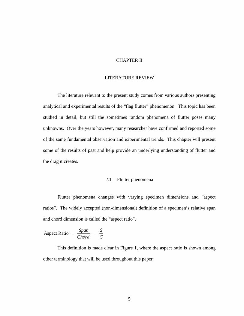
In addition to aspect ratio, a common non-dimensional mass property, called mass
ratio, is frequently used to categorize a specimen’s mass when comparing multiple test
specimens with varying aspect ratio parameters
air
mmrC
μρ
= =
:mass per area air densitychord length
wherem
cρ
===
7
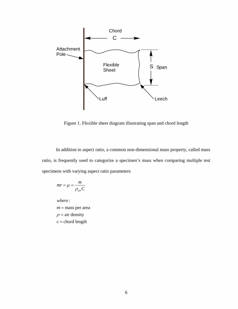
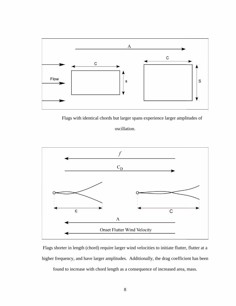
Fundamental Trends
To review the underlying physics of what has been learned from flag flutter
studies of past, a compilation of several fundamental research trends is presented below
in diagram form with underlying conclusions stated below the diagram.
Heavy flags oscillate at larger amplitudes, but at lower frequencies. Heavier flags
yield larger drag coefficients.
Flags with higher structural stiffness require higher wind speeds to initiate flutter
and flutter at lower amplitudes.
8
Flags with identical chords but larger spans experience larger amplitudes of
oscillation.
Flags shorter in length (chord) require larger wind velocities to initiate flutter, flutter at a
higher frequency, and have larger amplitudes. Additionally, the drag coefficient has been
found to increase with chord length as a consequence of increased area, mass.
9
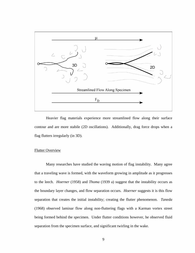
Heavier flag materials experience more streamlined flow along their surface
contour and are more stabile (2D oscillations). Additionally, drag force drops when a
flag flutters irregularly (in 3D).
Flutter Overview
Many researches have studied the waving motion of flag instability. Many agree
that a traveling wave is formed, with the waveform growing in amplitude as it progresses
to the leech. Hoerner (1958) and Thoma (1939 a) suggest that the instability occurs as
the boundary layer changes, and flow separation occurs. Hoerner suggests it is this flow
separation that creates the initial instability; creating the flutter phenomenon. Taneda
(1968) observed laminar flow along non-fluttering flags with a Karman vortex street
being formed behind the specimen. Under flutter conditions however, he observed fluid
separation from the specimen surface, and significant twirling in the wake.
10
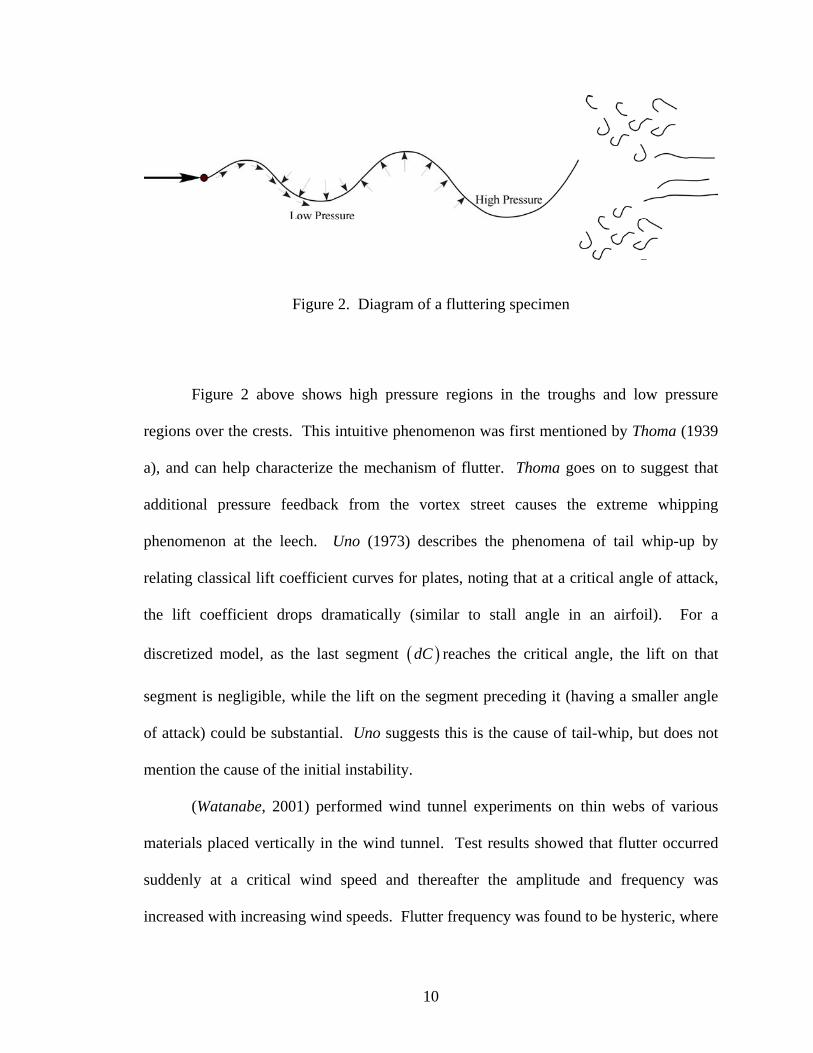
Figure 2. Diagram of a fluttering specimen
Figure 2 above shows high pressure regions in the troughs and low pressure
regions over the crests. This intuitive phenomenon was first mentioned by Thoma (1939
a), and can help characterize the mechanism of flutter. Thoma goes on to suggest that
additional pressure feedback from the vortex street causes the extreme whipping
phenomenon at the leech. Uno (1973) describes the phenomena of tail whip-up by
relating classical lift coefficient curves for plates, noting that at a critical angle of attack,
the lift coefficient drops dramatically (similar to stall angle in an airfoil). For a
discretized model, as the last segment ( )dC reaches the critical angle, the lift on that
segment is negligible, while the lift on the segment preceding it (having a smaller angle
of attack) could be substantial. Uno suggests this is the cause of tail-whip, but does not
mention the cause of the initial instability.
(Watanabe, 2001) performed wind tunnel experiments on thin webs of various
materials placed vertically in the wind tunnel. Test results showed that flutter occurred
suddenly at a critical wind speed and thereafter the amplitude and frequency was
increased with increasing wind speeds. Flutter frequency was found to be hysteric, where
11
the flag would become stable when ramped down at a wind speed about 25% lower than
its critical wind speed. For sheets with a larger chord length, the wind velocity at which
flutter occurred was lower than that of sheets of small chord lengths. Additionally
Watanabe found stiffer materials (EI), required faster wind speeds to initiate flutter than
those web materials that were thinner, having smaller mass ratios and structural stiffness.
Using a cable wire as the attachment support to conduct flutter experiments, Watanabe
found no significant air flow separation around the sheet, but significant disruptions in
the wake of the flutter (behind the flag). For web materials with relatively large thickness
(0.235 mm or greater) there was simple 2D flow (potential), while thinner materials
(0.028 mm or less) exhibited complex three dimensional flutter modes. That is for the
thicker sheets, the flow appeared to follow the contour of the waving motion, remaining
streamlined along the length of sheet and experiencing only small scale vortices
downstream of the luff. The thinner sheets however, experience three-dimensional
deformation, causing vortices to form along the deforming surface.
Drag Approximations
One of the first researcher to study induced drag, did so out of concern of thrust
for airplanes pulling large banners. Fairthorne (1930) performed an experimental study
of drag for large rectangular flags where most his published data was for a specimen with
a span of 4 ft.
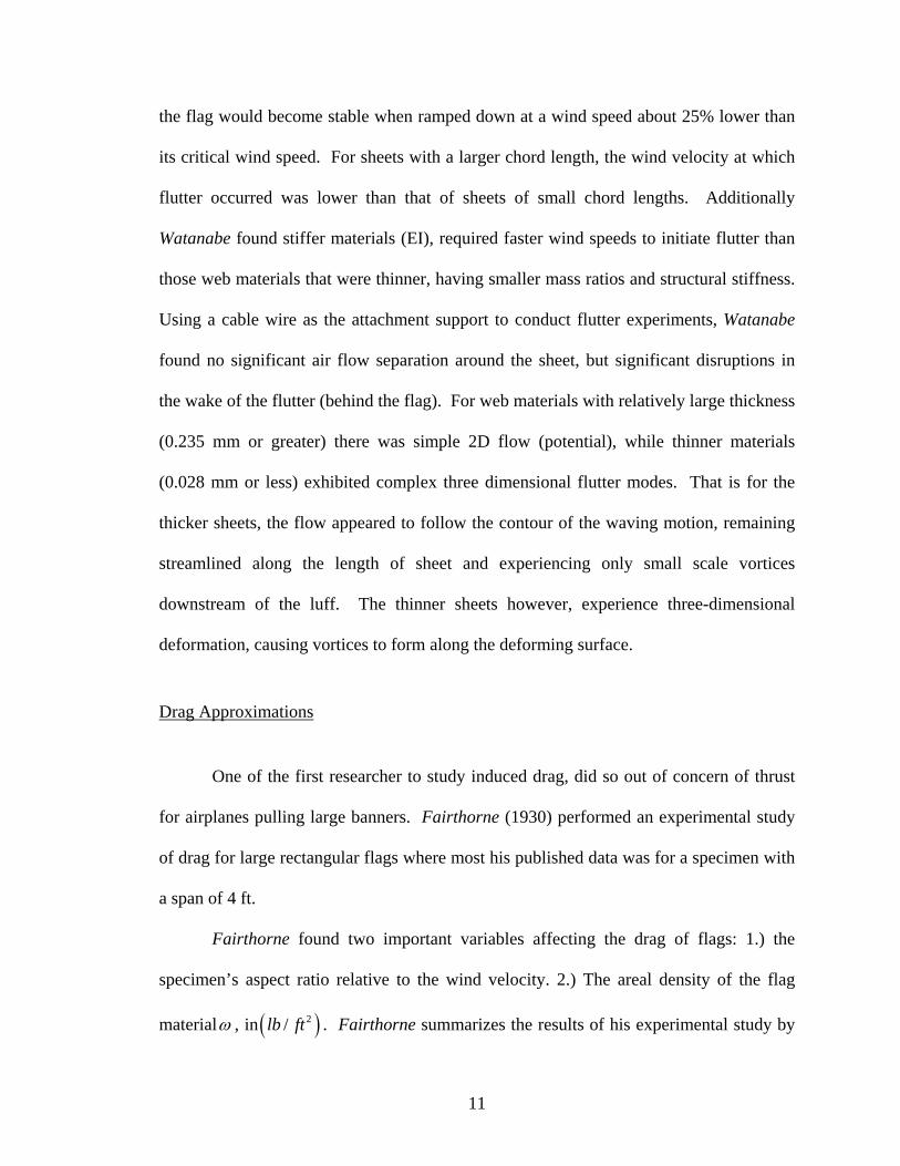
Fairthorne found two important variables affecting the drag of flags: 1.) the
specimen’s aspect ratio relative to the wind velocity. 2.) The areal density of the flag
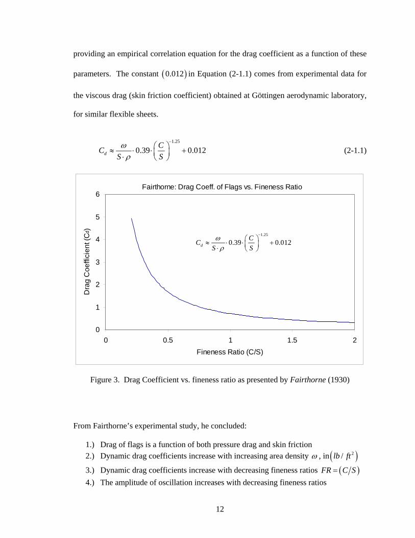
materialω , in ( )2/lb ft . Fairthorne summarizes the results of his experimental study by
12
providing an empirical correlation equation for the drag coefficient as a function of these
parameters. The constant ( )0.012 in Equation (2-1.1) comes from experimental data for
the viscous drag (skin friction coefficient) obtained at Göttingen aerodynamic laboratory,
for similar flexible sheets.
1.25
0.39 0.012dCC
S Sω
ρ
−⎛ ⎞≈ ⋅ ⋅ +⎜ ⎟⋅ ⎝ ⎠
(2-1.1)
Fairthorne: Drag Coeff. of Flags vs. Fineness Ratio
0
1
2
3
4
5
6
0 0.5 1 1.5 2Fineness Ratio (C/S)
Dra
g C
oeffi
cien
t (C
d ) 1.25
0.39 0.012dCC
S Sω
ρ
−⎛ ⎞≈ ⋅ ⋅ +⎜ ⎟⋅ ⎝ ⎠
Figure 3. Drag Coefficient vs. fineness ratio as presented by Fairthorne (1930)
From Fairthorne’s experimental study, he concluded:
1.) Drag of flags is a function of both pressure drag and skin friction 2.) Dynamic drag coefficients increase with increasing area density ω , in ( )2/lb ft
3.) Dynamic drag coefficients increase with decreasing fineness ratios ( )FR C S= 4.) The amplitude of oscillation increases with decreasing fineness ratios

13
5.) Flutter frequency of flag increases with decreasing fineness ratios 6.) Drag coefficients are nearly independent of the free stream Reynolds number for
flags of the tested geometric type (fineness ratio).
Shifting the discussion from empirical correlations with approximations deduced
analytically from physics; Moretti (2003) suggests that the large curvature of the fabric at
the leech, as a result of the flutter motion, generates centrifugal forces that induce the
largest tension (drag) force at the attachment. From Thoma’s paper (1939 b) of tension in
a rope, Moretti postulates a closed form time averaged approximation of drag for a
fluttering flag.
Thoma (1939 b) expresses the average tension per unit segment ( )ds in a rope as:
( )2
2fmdT d V
ds ds= − i (2-1.2)
Upon integration, and applying the bounds over a flag length ( )s L= :
212 flag leechT m V= (2-1.3)
which is to say that the largest effect of tension comes from the kinetic energy
dissipation at the leech, where the velocity is a maximum. Moretti goes on to
approximate the average tension at the luff (attachment pole), by differentiating an
assumed deflection profile (waveform) and inserting the velocity (evaluated at the leech)
into Equation (2-1.3). Assuming a simplified waveform motion (deflection) as
cos( )Axz t kxL
ω= − , Moretti (2003) predicts the average dynamically induced tension in
a flag by Equation (2-1.4).
2 214 flagT m A ω= (2-1.4)
14
:mass-per-unit-length
amplitude at the leech (half )circular frequency (rad/s)
flag
wherem
Aω
=
==
For stiff panels (incapable of flutter) drag is produced from skin friction acting
along both surfaces. Hoerner (1958) found the skin friction drag coefficient to be very
low; typically in the order of 0.01dC ≈ . The dynamic effect of a fluttering flag however,
has proven to gives rise to much larger drag forces than just skin friction alone. Moretti
(2003) postulates that not only is the dynamic tension significantly larger, but is also
distributed much more broadly over the specimen length. Comparing the relative
contribution and distribution of drag per unit length produced from a flexible specimen,
Moretti creatively non-dimensionalizes laminar skin friction as:
2 1.328 air air
air
T L xL U UL L
μ ρρ
⎡ ⎤−≅ ⎢ ⎥
⎣ ⎦i
and the dynamically induced tension distribution from Equation (2-1.4) as:
2
2 2
1 14flag
T xm A Lω
⎡ ⎤⎛ ⎞≅ −⎢ ⎥⎜ ⎟⎝ ⎠⎢ ⎥⎣ ⎦
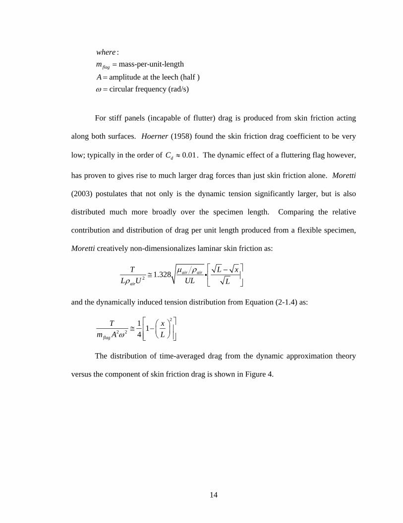
The distribution of time-averaged drag from the dynamic approximation theory
versus the component of skin friction drag is shown in Figure 4.
15
Flag Drag Distribution
0
0.1
0.2
0 2 4 6 8 10 12 14Flag Dimension (in.)
Dra
g D
istri
butio
n
Dynamic Drag--MorettiLaminar Skin Friction
Skin Friction Distribution
Figure 4. Relative magnitude and distribution of dynamically induced tension vs. skin friction (viscous) drag.
Clearly, the dynamically induced tension prediction yields a much broader
distribution of drag over the length of the specimen, with the maximum drag occurring at
the attachment pole ( )0x = and tapering to zero at the leech. The drag imposed by
viscous skin friction, yields a small spike at the luff and quickly tapers toward zero, thus
further confirming the minute contribution of drag in comparison with dynamic
approximations.

16
CHAPTER III
THEORIES
3.1 Fundamentals of Drag and Lift
Classical Drag of a cylinder in a fluid stream
Pressure drag is the drag associated with the pressure disturbance of the fluid as it
passes over a body and separates into a turbulent wake. Pressure drag is a function of the
shape/orientation of the body, the surface quality of the object, and the fluid’s Reynolds
number. Pressure drag is sometimes referred to as form drag, because significant drag
variations can occur by changing the form (shape) of the object Mott (2000). A
streamlined object effectively changes the separation point of the boundary layer,
creating a smaller wake, and thus reducing the net drag force. Additionally, the
roughness of the objects surface can significantly affect the separation point of the fluid
at different Reynolds numbers. A rough surface finish changes the nature of the fluid
boundary layer from laminar to turbulent at lower Reynolds numbers, moving the
separation point further back on the body, decreasing the size of the turbulent wake, and
thus decreasing the drag force at lower Reynolds numbers. A second component of drag,
friction drag, can be found by integrating the shear stress distribution along the object’s
surface. It is this shearing force, between the object and the fluid stream, that decelerates
the fluid near the object’s surface, thus creating a boundary layer. At very low Reynolds

17
numbers, ( )Re 1< the drag is due almost entirely to friction, while at higher Reynolds
numbers flow separation and the turbulence in the wake of the object make pressure drag
predominant Mott (2000). Classically, drag forces are expressed in the form
20
12D DF C U Aρ⎛ ⎞= ⎜ ⎟
⎝ ⎠ (3-1.1)
0
:drag coefficient
density of the fluidfreestream fluid velocity
characteristic area of the body
D
whereC
UA
ρ=
==
=
The drag coefficient ( )DC is a dimensionless number based on the shape of the
body and its orientation to the fluid stream. The characteristic area ( )A is the effective
frontal area perpendicular to the free stream flow. The combined term 212
vρ⎛ ⎞⎜ ⎟⎝ ⎠
, is called
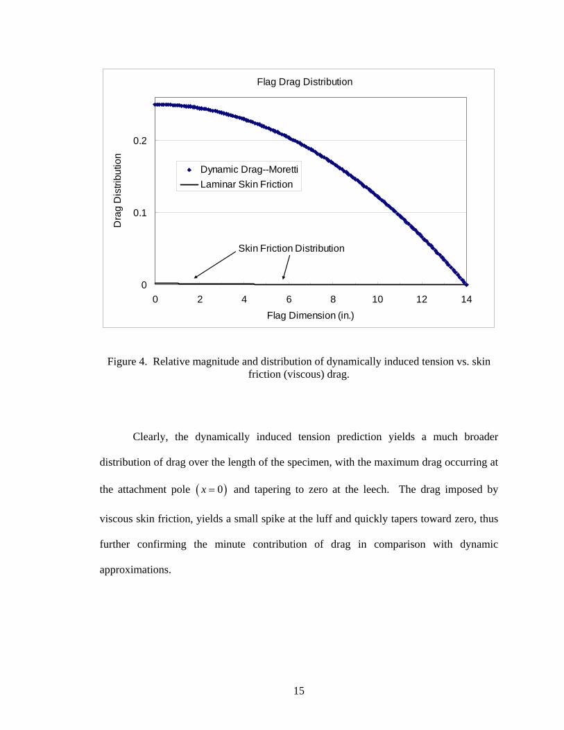
the dynamic pressure and comes from Bernoulli’s equation. Consider the classical case
of a cylinder oriented with its axial axis perpendicular to a cross flow as shown in Figure
5. As the fluid stream hits the surface of the object ( )at location sp , the velocity of the
fluid stops thus creating a “stagnation point” and a corresponding stagnation
pressure ( )sp . This point creates the largest pressure differential from free stream static
pressure ( )1p .
18
Figure 5 Cross-section of a cylinder in a fluid stream
The relationship between these two pressures can be found from Bernoulli’s equation as
follows:
( )22
1 111.
2 2s s
sp vp vz z
g gγ γ+ + = + +
Where: elevation is constant and the fluid velocity is zero at location ( ), 0ss v = , giving:
( )2
1 12. 2
spp vgγ γ
+ =
Solving for the stagnation pressure and substitutinggγρ = , the stagnation pressure (total
pressure) is greater than the static pressure in the free stream by the magnitude of the
dynamic pressure 21
12
vρ⎛ ⎞⎜ ⎟⎝ ⎠
.
( ) 21 1
13. 2sp p vρ= + (3-1.2)
19
The increased pressure at the stagnation point and the sudden pressure drop in the
fluid wake behind the object creates an unbalance of pressures around the body, thus
creating a reactive force opposing the fluid motion. The magnitude of this drag force
(pressure drag) not only depends on the free stream static pressure ( )1p and the
stagnation pressure ( )sp , but also on the pressure in the wake of the object. Because the
turbulence of the fluid in the wake is unsteady and hard to predict, a constant coefficient
(a drag coefficient based on experimental data, DC ) is used to adjust drag calculations.
Experimental drag coefficient data is commonly presented in texts as a plot of the drag
coefficient on the ordinate versus the Reynolds number on the abscissa. The Reynolds
number calculation is unique to the geometry of the object. Instead of using the fluid
conduit diameter or hydraulic radius to compute the Reynolds number, the dimension of
the body parallel to the fluid stream is used when referencing drag coefficient data from
charts.
( )
0Re U Dμ ρ
= (3-1.3)
0
:density of fluid streamfree stream fluid velocity
characteristic dimension (diameter for cylinders)dynamic viscosity of fluid steam
where
UD
ρ
μ
==
==
As is evident from Equations (3-1.1) and (3-1.3), it becomes critical to understand
the properties of the fluid (air), which consequently is time dependent. As with all gases,
20
the properties of air change with temperature and altitude. Using a mercury barometer,
the local atmospheric pressure can be computed as:
( )atm Hg barometerp g hρ= (3-1.4)
:density of mercury
ravitational accelerationheight of mercury
Hg
barometer
where
g gh
ρ =
==
and with the local atmospheric pressure, the density of air can be computed as:
atmair
abs
pRT
ρ = (3-1.5)
:local atmosheric pressure
univeral gas constantabsolute temperature
atm
abs
wherepRT
==
=
The Sutherland equation can be used to compute the dynamic viscosity of the air by
measuring the local temperature.
1
absoluteair
absolute
b T
ST
μ =⎡ ⎤⎛ ⎞
+⎢ ⎥⎜ ⎟⎝ ⎠⎣ ⎦
(3-1.6)
61 2
:
1.458 10
110.4 absolute local temperatureabsolute
wherekgb
m s KS KT
−= ×− −
==
An excel spreadsheet calculator (courtesy of F.W. Chambers), was used to compute air
properties from barometer temperature and pressure readings. This sheet and related

21
formulae are shown in Appendices I-J. Combining the physical properties from above,
the drag force on a cylinder subject to a cross flow is defined as:
20
12cylinderD D airF C U DLρ⎛ ⎞= ⎜ ⎟
⎝ ⎠ (3-1.7)
( )( )
0
0
:
Re for circular cylinder
drag coefficient Re (from experimentally published data)
density of fluid streamfree stream fluid velocity
diameter of cylinder (flag pole)
D
D D D
air
whereU D
C C f
UDL
μ ρ
ρ
=
= =⎡ ⎤⎣ ⎦=
=
== length of cylinder normal to fluid stream
From tables, a smooth cylinder has a drag coefficient
3 41.0 for 10 Re 10D DC ≈ ≤ ≤ . Figure 6 compares theoretical drag data for a classical
cylinder in a cross-flow with that measured experimentally for the attachment pole. The
attachment pole; with diameter 0.375 0.0127 D in m= = , and length
36 0.939 L in m= = is a smooth stainless steel rod. A center “half section” of the rod is
removable and serves to clamp various test specimens. Screw recesses were filled with
putty to keep the round contour and thin scotch tape was placed over the leading edge of
joint. A picture of the attachment pole is given in Figure 18 on page 40.
22
Classical Cylinder Drag
0
0.05
0.1
0.15
0.2
0.25
0.3
0.35
0.4
0 1 2 3 4 5 6 7 8 9 10 11 12 13 14 15 16 17Velocity (m/s)
Dra
g (lb
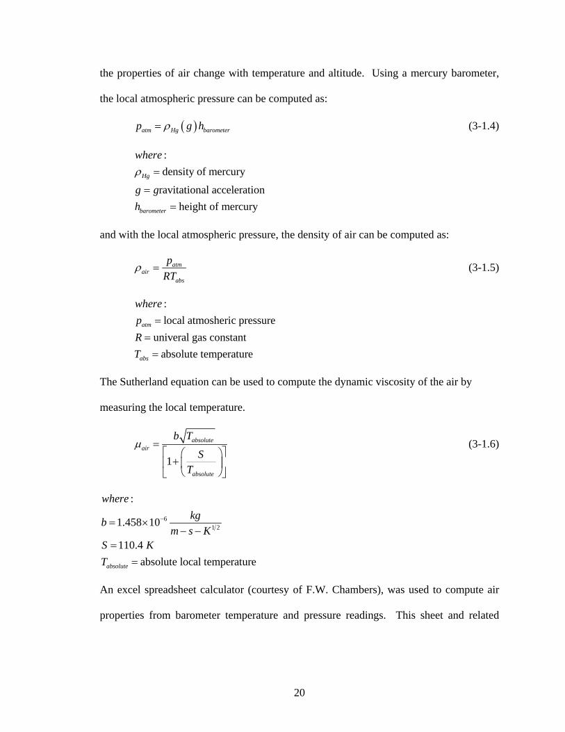
f)TheoryExp.
Figure 6. Theoretical and experimental profile of drag vs. velocity for a circular cylinder ( )1.0DC =
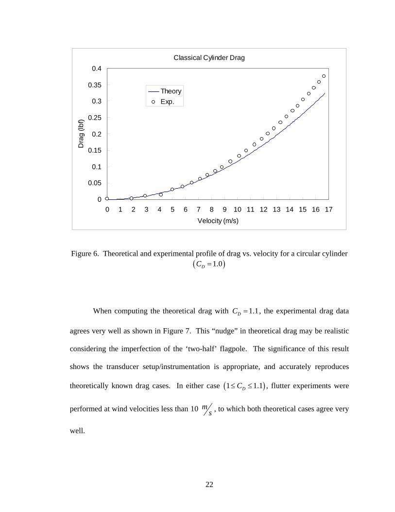
When computing the theoretical drag with 1.1DC = , the experimental drag data
agrees very well as shown in Figure 7. This “nudge” in theoretical drag may be realistic
considering the imperfection of the ‘two-half’ flagpole. The significance of this result
shows the transducer setup/instrumentation is appropriate, and accurately reproduces
theoretically known drag cases. In either case ( )1 1.1DC≤ ≤ , flutter experiments were
performed at wind velocities less than 10 ms , to which both theoretical cases agree very
well.
23
Classical Cylinder Drag
0
0.05
0.1
0.15
0.2
0.25
0.3
0.35
0.4
0 1 2 3 4 5 6 7 8 9 10 11 12 13 14 15 16 17Velocity (m/s)
Dra
g (lb
f)Theory--Cd=1.1Exp.
Figure 7. Experimental accuracy with a known drag case
Classical Lift
The drag force in the previous section was defined as the force acting parallel to
the fluid stream, and now we consider the component of the force that acts perpendicular
to the fluid stream. This lift force is present on objects placed in a fluid stream at an
angular referenceα , with respect to a characteristic chord. Consider the cross section of
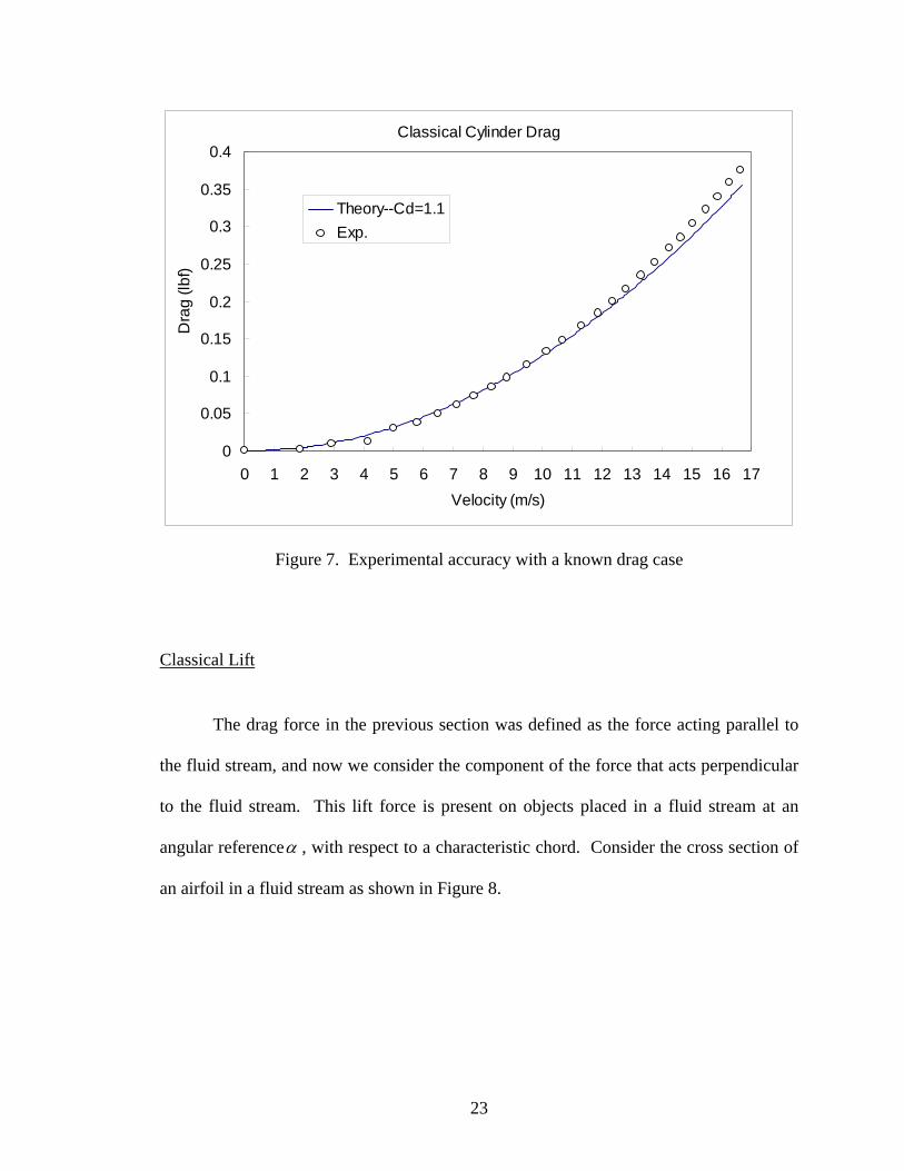
an airfoil in a fluid stream as shown in Figure 8.

24
Figure 8. Classical airfoil diagram of forces
The airfoil placed at an “attack angle” α , is subject to two component forces: lift
and drag. As the fluid hits the underside of the foil, pressure forces act normal to the
surface contour. These normal pressure forces, net drag, are resolved into component x
and y forces. The vertical component of force is lift, and the horizontal component is the
drag. Both of which, are a result (dependent) of the object’s angular orientation to the
fluid stream α . It should be emphasized, that the induced component of force is a
consequence of lift forces, generated by the fluid stream or other external lift forces.
3.2 Stiff Vane Drag in a Fluid Stream
For the second phase of experimentation, a rigid panel ( 116"aluminum sheet),
incapable of flutter, was attached to the pole. The panel was oriented such that its planar
surface was parallel to the flow stream. In comparison to the cylinder in a cross flow
(flag pole only), we anticipate a larger net drag force due to the addition of skin-friction
Induced Drag
Vector (Net) Drag Lift
Flow
α
25
(viscous drag), caused by the shearing stress within the thin boundary layer along the
stationary plate. That is, the net drag force for the rigid panel connected to the flagpole
will be a function of pressure drag (form drag from the flagpole), and viscous drag (skin-
friction drag from the rigid panel: ( )Rigid PanelD Dp DvF F F= + . Recall from the previous
section, the pressure drag of the flagpole is defined as:
( ) 20
12cylinderD D air DpF C U DL Fρ⎛ ⎞
⎜ ⎟⎝ ⎠
= = .
Laminar Boundary Layer
Now we will consider the viscous drag on the rigid panel, DvF . Because the stiff
panel is a streamlined object, we expect the fluid to attach to the surface of the panel
reducing the turbulence associated with blunt body objects. This streamlined effect
creates a thin film boundary along the surface of the panel, known as the boundary layer.
The layer of fluid in the boundary layer has undergone a change in velocity as a result of
the shearing stress at the surface. Traditionally, the boundary layer on the flat panel starts
at the leading edge of the panel and grows in thickness along the length of the panel until
the fluid stream becomes unstable and separated into a turbulent boundary layer. For the
traditional case of only a flat panel subject to a flow stream where 5Re 10L < , and
assuming the velocity distribution along the panel does not vary ( )0dp dx = , the
frictional resistance (drag) due to viscous shearing in a laminar boundary layer can be
computed as follows:

26
Given the classical relationship of shear stress relating absolute viscosity and the velocity
gradient of the boundary:
0dudy
τ μ= (3-2.1)
The velocity gradient for a laminar boundary layer is approximated as:
1200.332 ReL
Ududy x
=
And the shear stress at the boundary becomes:
120
0 0.332 ReLUx
τ μ=
The shearing force on one side of the plate can be written as:
120
0 0 0.332 Re
L
D LA
UF dA w dxx
τ μ= =∫ ∫
( ) 12
00.664 ReD LpanelF w Uμ= (3-2.2)
( )
0
0
:panel widthdynamic viscosityfree stream fluid velocity
Re/L
wherew
UU L
μ
μ ρ
===
=
A dimensionless shear stress coefficient can be presented as:
0
20
12
fcU
τ
ρ=
And from above, the localized drag force becomes:
2
2 00
1 2 2D f f
A A
UF c U dA c dAρρ⎛ ⎞= =⎜ ⎟⎝ ⎠∫ ∫
27
In terms of an average shear stress coefficient, we have:
2
0
2
fD A
c dAUF
wL wLρ
⎡ ⎤⎢ ⎥
= ⎢ ⎥⎢ ⎥⎣ ⎦
∫
And the average shear stress coefficient becomes:
( )2
0 2
fA D
f
c dAFC
wL wL Uρ
⎡ ⎤⎢ ⎥
= =⎢ ⎥⎢ ⎥⎣ ⎦
∫ (3-2.3)
Combining Equations (3-2.2) and (3-2.3):
( )
12
0
1.328 1.328 Re
/
fL
CU Lμ ρ
= = (3-2.4)
The generalized viscous drag force for a flat plate subject to drag along both faces can be written as:
( ) 20
122D f airpanel
F C U wLρ⎡ ⎤⎛ ⎞= ⎜ ⎟⎢ ⎥⎝ ⎠⎣ ⎦
And the total viscous drag on a flat plate with a laminar boundary layer is:
( ) ( )2
0D f airpanelF C U wLρ⎡ ⎤= ⎣ ⎦ (3-2.5)
( )
12
0
0
:1.328 , average laminar boundary layer viscous friction coefficientRe
Re , reynolds number given by the panel chord length/
density of fluid streamfree stream fluid velocity
pa
fL
L
air
where
C
U L
Uw
μ ρρ
=
=
==
= nel widthpanel lengthL =

28
Turbulent Boundary Layer
By applying momentum equations to a turbulent boundary layer, detailed by
Roberson (1997), the average turbulent boundary layer viscous friction coefficient for a
flat plate can be expressed as:
15
70.074 for Re 10Ref
L
C = < (3-2.6)
The skin friction due to the turbulent boundary layer from equation (3-2.6) above, can be
inserted into the generalized viscous drag force given by equation (3-2.5). The total
viscous drag on a flat plate with a turbulent boundary layer 7(Re 10 )< is:
( ) ( )20D f airpanel
F C U wLρ⎡ ⎤= ⎣ ⎦ (3-2.7)
15
0
:0.074 , average turbulent boundary layer viscous friction coefficientRedensity of fluid stream
free stream fluid velocitypanel widthpanel length
fL
air
where
C
UwL
ρ
=
==
==
29
Drag vs Wind VelocityStiff Vane
0
0.02
0.04
0.06
0.08
0.1
0.12
0.14
0.16
0.18
0.2
0 5 10 15 20 25 30 35Velocity (m/s)
Dra
g (L
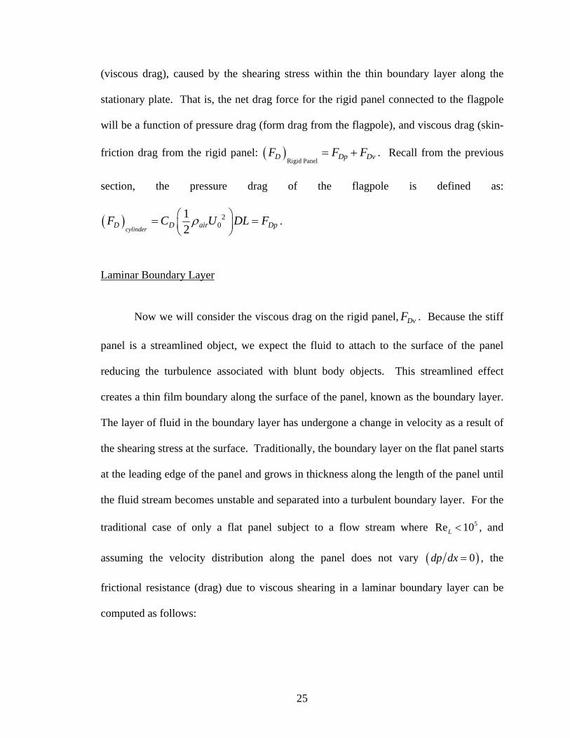
bf)
Drag -turbulentDrag -laminar
Figure 9 Comparison of laminar and turbulent boundary layer drag for a stiff panel.
From the plot in Figure 9 we see that the viscous drag on a stiff vane is dependent
on the boundary layer type. A turbulent boundary layer will produce a higher drag force
than that for a laminar boundary layer along the surface of the plate. Noting the ordinate
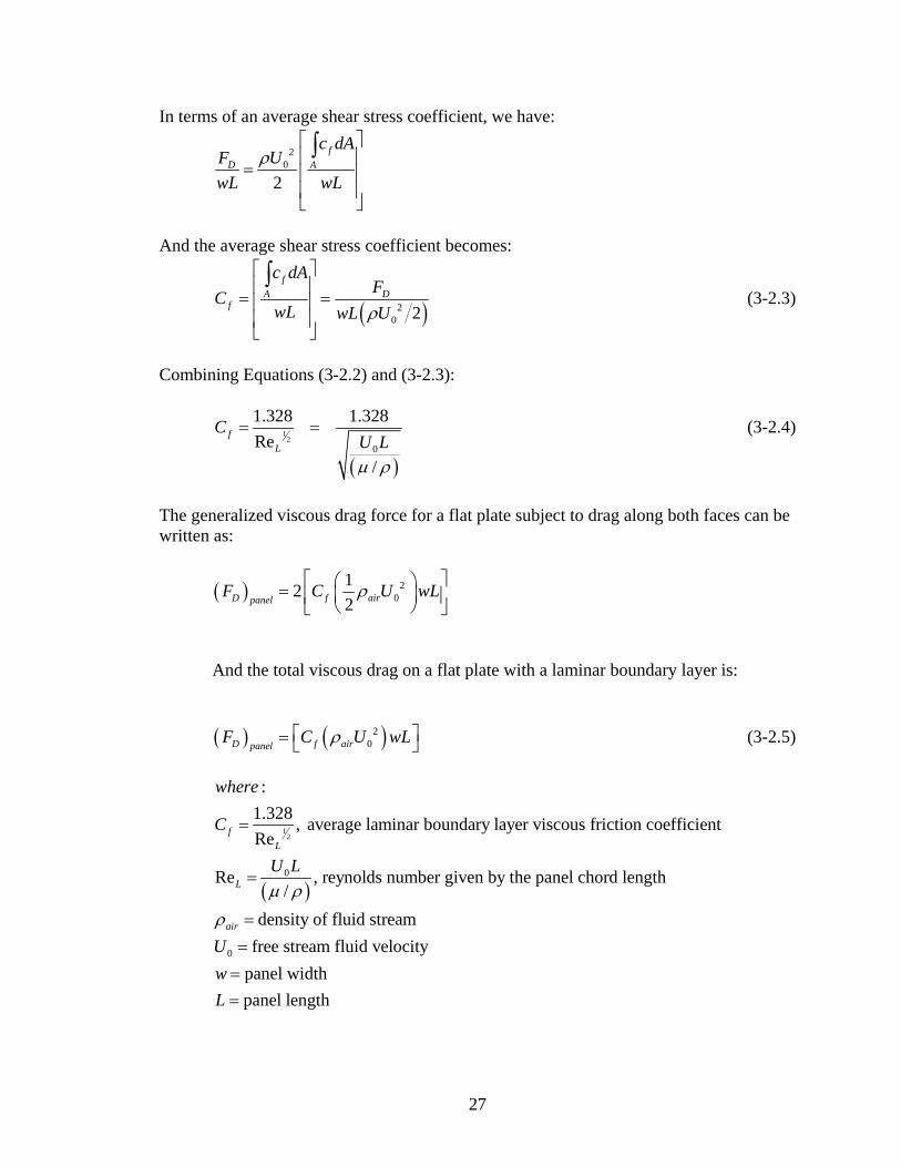
scale, we see that viscous drag (skin friction) is small in magnitude even over a large
free-stream velocity range. This point is emphasized in Figure 10, where the effects of
the pressure drag from the pole dominate the net drag force for a pole with a stiff vane
attachment.
30
Net Drag Force for a Stiff Vane Attached to a Pole
0
0.25
0.5
0.75
1
1.25
1.5
1.75
2
2.25
0 5 10 15 20 25 30 35Velocity (m/s)
Dra
g (L
bf)
Pole+Turbulent
Pole+Laminar
Figure 10 Combined Drag force of pole and stiff vane attachment
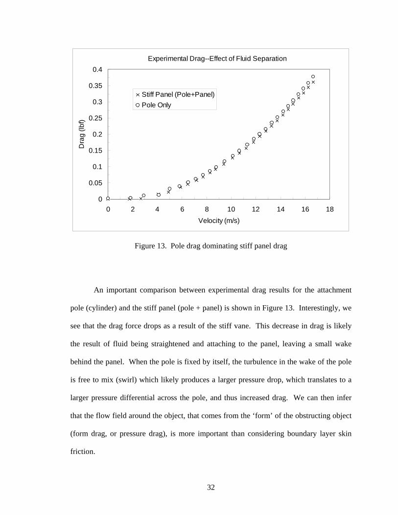
Experiments for the stiff panel were completed with a 116 .in thick sheet of
aluminum, with identical dimensions for the fabrics tested in proceeding sections. Figure
11 shows the chord and span dimension used for every test case. Additionally, the stiff
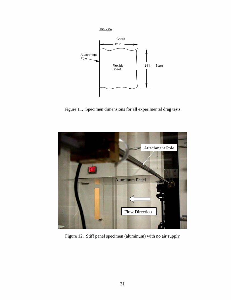
panel setup is shown in its tested condition in Figure 12.
31
FlexibleSheet
Chord
Span
AttachmentPole
14 in.
12 in.
Top View
Figure 11. Specimen dimensions for all experimental drag tests
Aluminum Panel
Attachment Pole
Flow Direction
Figure 12. Stiff panel specimen (aluminum) with no air supply
32
Experimental Drag--Effect of Fluid Separation
0
0.05
0.1
0.15
0.2
0.25
0.3
0.35
0.4
0 2 4 6 8 10 12 14 16 18Velocity (m/s)
Dra
g (lb
f)
Stiff Panel (Pole+Panel)Pole Only
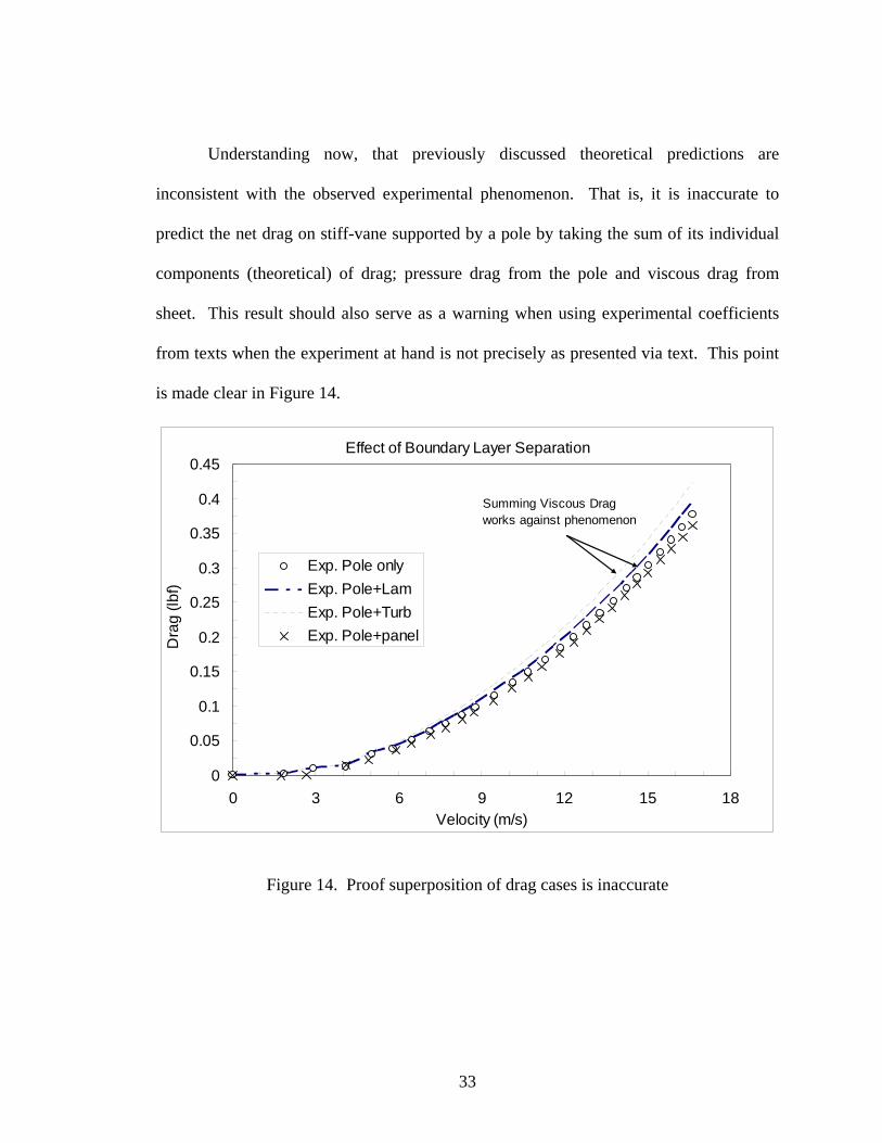
Figure 13. Pole drag dominating stiff panel drag
An important comparison between experimental drag results for the attachment
pole (cylinder) and the stiff panel (pole + panel) is shown in Figure 13. Interestingly, we
see that the drag force drops as a result of the stiff vane. This decrease in drag is likely
the result of fluid being straightened and attaching to the panel, leaving a small wake
behind the panel. When the pole is fixed by itself, the turbulence in the wake of the pole
is free to mix (swirl) which likely produces a larger pressure drop, which translates to a
larger pressure differential across the pole, and thus increased drag. We can then infer
that the flow field around the object, that comes from the ‘form’ of the obstructing object
(form drag, or pressure drag), is more important than considering boundary layer skin
friction.
33
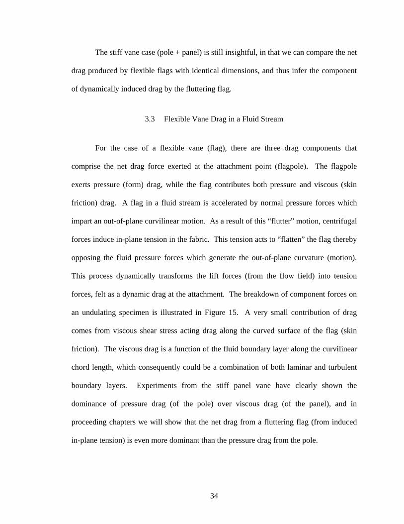
Understanding now, that previously discussed theoretical predictions are
inconsistent with the observed experimental phenomenon. That is, it is inaccurate to
predict the net drag on stiff-vane supported by a pole by taking the sum of its individual
components (theoretical) of drag; pressure drag from the pole and viscous drag from
sheet. This result should also serve as a warning when using experimental coefficients
from texts when the experiment at hand is not precisely as presented via text. This point
is made clear in Figure 14.
Effect of Boundary Layer Separation
0
0.05
0.1
0.15
0.2
0.25
0.3
0.35
0.4
0.45
0 3 6 9 12 15 18Velocity (m/s)
Dra
g (lb
f)
Exp. Pole onlyExp. Pole+LamExp. Pole+TurbExp. Pole+panel
Summing Viscous Dragworks against phenomenon
Figure 14. Proof superposition of drag cases is inaccurate
34
The stiff vane case (pole + panel) is still insightful, in that we can compare the net
drag produced by flexible flags with identical dimensions, and thus infer the component
of dynamically induced drag by the fluttering flag.
3.3 Flexible Vane Drag in a Fluid Stream
For the case of a flexible vane (flag), there are three drag components that
comprise the net drag force exerted at the attachment point (flagpole). The flagpole
exerts pressure (form) drag, while the flag contributes both pressure and viscous (skin
friction) drag. A flag in a fluid stream is accelerated by normal pressure forces which
impart an out-of-plane curvilinear motion. As a result of this “flutter” motion, centrifugal
forces induce in-plane tension in the fabric. This tension acts to “flatten” the flag thereby
opposing the fluid pressure forces which generate the out-of-plane curvature (motion).
This process dynamically transforms the lift forces (from the flow field) into tension
forces, felt as a dynamic drag at the attachment. The breakdown of component forces on
an undulating specimen is illustrated in Figure 15. A very small contribution of drag
comes from viscous shear stress acting drag along the curved surface of the flag (skin
friction). The viscous drag is a function of the fluid boundary layer along the curvilinear
chord length, which consequently could be a combination of both laminar and turbulent
boundary layers. Experiments from the stiff panel vane have clearly shown the
dominance of pressure drag (of the pole) over viscous drag (of the panel), and in
proceeding chapters we will show that the net drag from a fluttering flag (from induced
in-plane tension) is even more dominant than the pressure drag from the pole.
35
( )Dv xF
( )Dv yF ( )Dp y
F( )Dp flagF
( )Viscous Drag DvF
High PressureLow Pressure
Lift Force
Induced Tension
Flag Pressure Force
( )D totalF
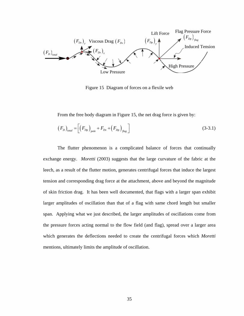
Figure 15 Diagram of forces on a flexile web
From the free body diagram in Figure 15, the net drag force is given by:
( ) ( ) ( )D Dp Dv Dptotal pole flagF F F F⎡ ⎤= + +
⎣ ⎦ (3-3.1)
The flutter phenomenon is a complicated balance of forces that continually
exchange energy. Moretti (2003) suggests that the large curvature of the fabric at the
leech, as a result of the flutter motion, generates centrifugal forces that induce the largest
tension and corresponding drag force at the attachment, above and beyond the magnitude
of skin friction drag. It has been well documented, that flags with a larger span exhibit
larger amplitudes of oscillation than that of a flag with same chord length but smaller
span. Applying what we just described, the larger amplitudes of oscillations come from
the pressure forces acting normal to the flow field (and flag), spread over a larger area
which generates the deflections needed to create the centrifugal forces which Moretti
mentions, ultimately limits the amplitude of oscillation.
36
CHAPTER IV
EXPERIMENTAL STUDY
In this chapter, the methods used to capture various experimental variables, the
procedure used, and the results are presented. This chapter is organized into five
sections. Section 4.1 presents the experimental setup, specifically designed for the study
of drag forces imparted from an attachment specimen. This section further discusses the
experimental methods used to capture/compute each experimental variable. Section 4.2
provides a step-by-step procedure used to capture experimental data for each test
specimen. Section 4.3 describes the estimation of uncertainty of the experimental drag
data. Finally, the experimental results are presented in Section 4.4.
4.1 Experimental Setup
Wind Tunnel Test Section
Wind tunnel experimentation was performed using a downdraft wind tunnel and a
removable test section with a 3 3 ft× cross-section. A new section was designed and
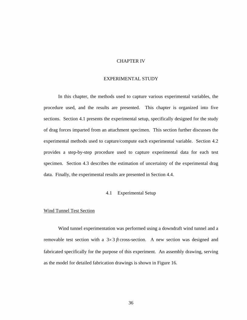
fabricated specifically for the purpose of this experiment. An assembly drawing, serving
as the model for detailed fabrication drawings is shown in Figure 16.
37
Figure 16 Wind tunnel test section illustration with specimen and pitot tube probe.
The removable test section features rigid mounting pillars for load cell
attachment, pitot tube traverse, half panel access door, adjustable vibration damping feet,
and acrylic viewing panels. The section was constructed of three-inch angle iron and has
a step-less inner cross-section. The angle iron section serves as a ‘shell’ for the routered
edges of the acrylic panels to fit snugly into place. The base of the test section was
constructed of two inch square tubing and has one open side for easy user/equipment
access. Detailed part lists and assembly drawings can be found in Appendix A. The
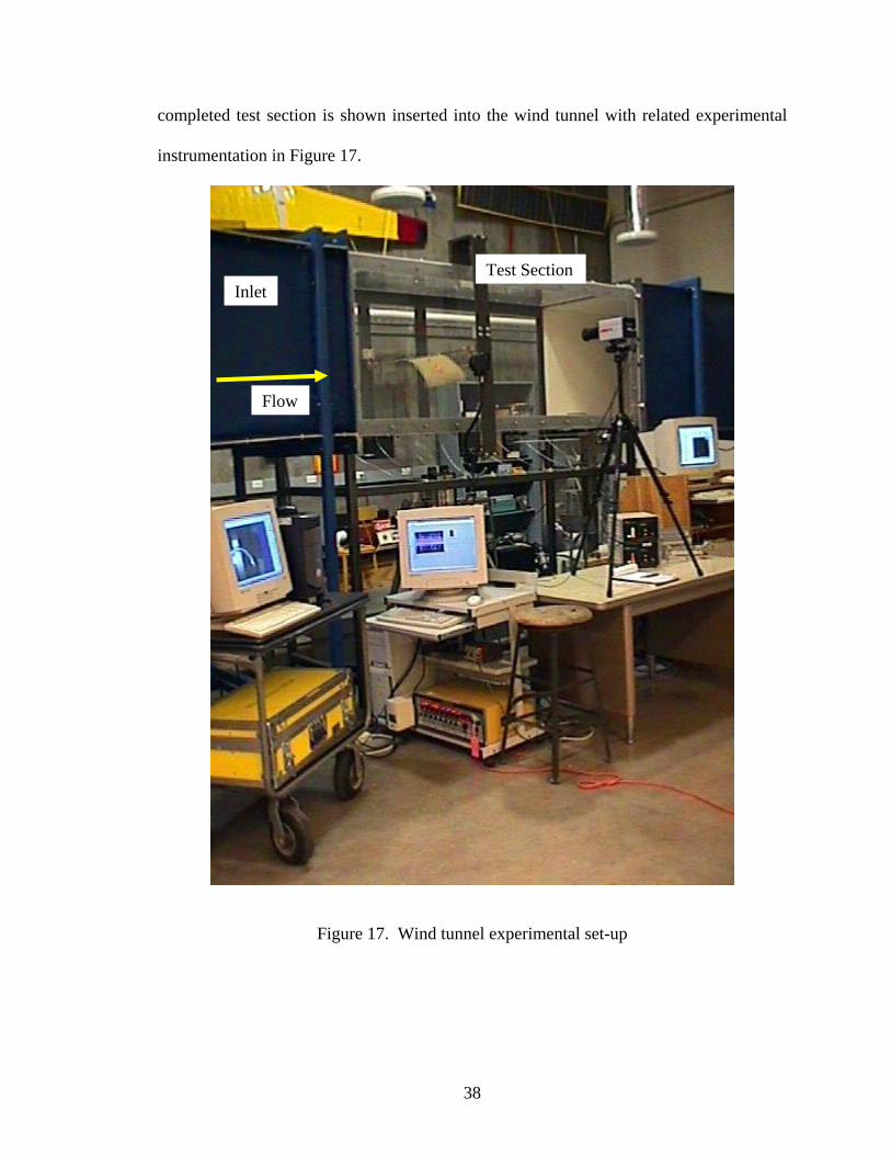
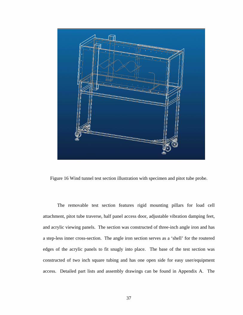
38
completed test section is shown inserted into the wind tunnel with related experimental
instrumentation in Figure 17.
Figure 17. Wind tunnel experimental set-up
Inlet Test Section
Flow
39
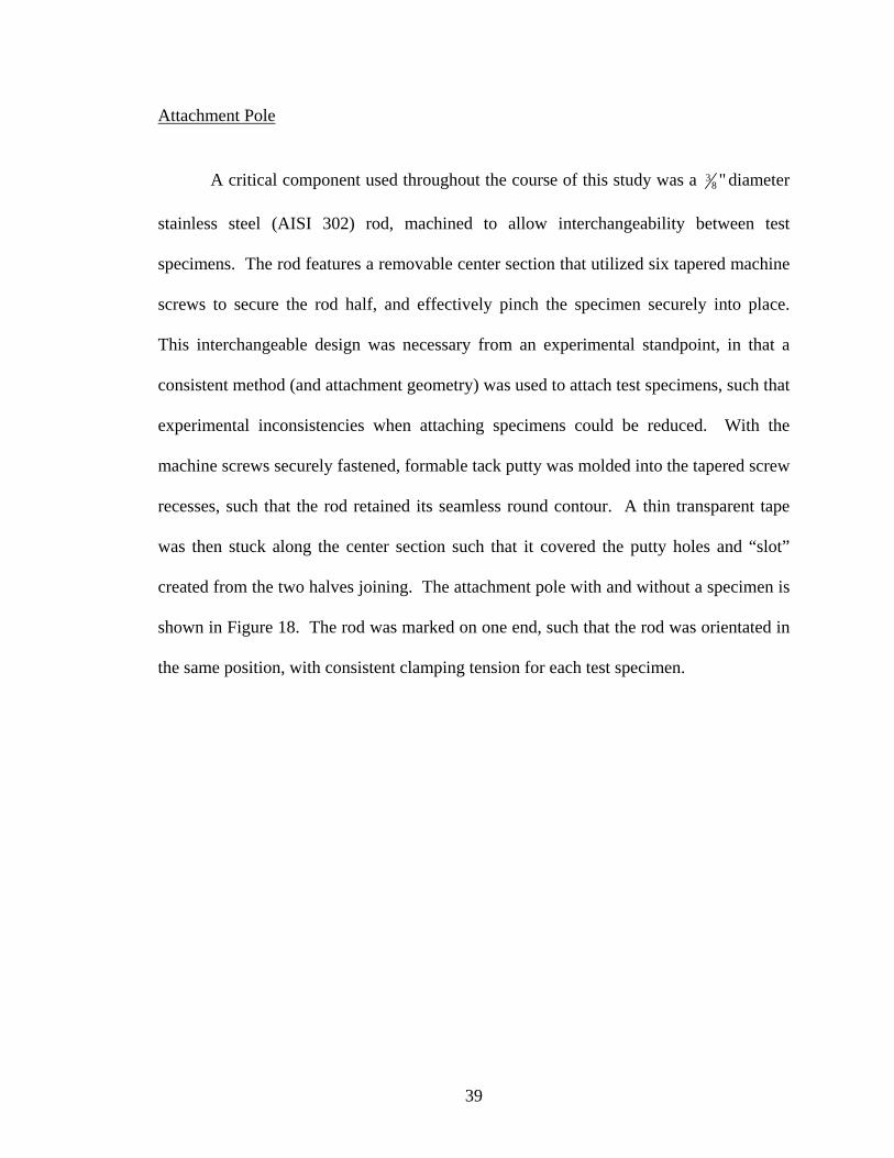
Attachment Pole
A critical component used throughout the course of this study was a 38 " diameter
stainless steel (AISI 302) rod, machined to allow interchangeability between test
specimens. The rod features a removable center section that utilized six tapered machine
screws to secure the rod half, and effectively pinch the specimen securely into place.
This interchangeable design was necessary from an experimental standpoint, in that a
consistent method (and attachment geometry) was used to attach test specimens, such that
experimental inconsistencies when attaching specimens could be reduced. With the
machine screws securely fastened, formable tack putty was molded into the tapered screw
recesses, such that the rod retained its seamless round contour. A thin transparent tape
was then stuck along the center section such that it covered the putty holes and “slot”
created from the two halves joining. The attachment pole with and without a specimen is
shown in Figure 18. The rod was marked on one end, such that the rod was orientated in
the same position, with consistent clamping tension for each test specimen.
40
Figure 18. Attachment pole
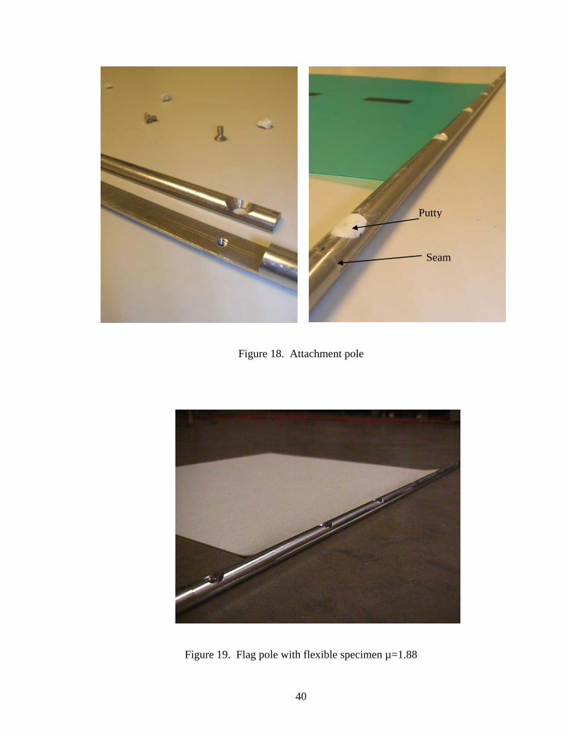
Figure 19. Flag pole with flexible specimen µ=1.88
Putty
Seam
41
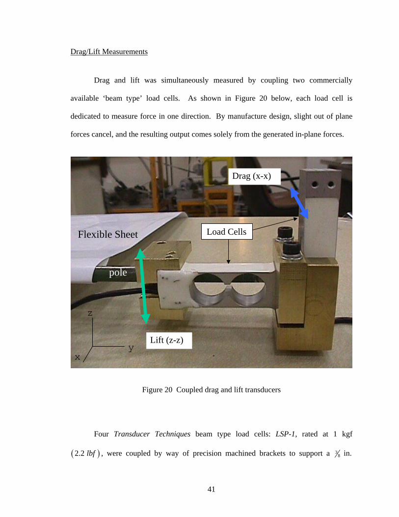
Drag/Lift Measurements
Drag and lift was simultaneously measured by coupling two commercially
available ‘beam type’ load cells. As shown in Figure 20 below, each load cell is
dedicated to measure force in one direction. By manufacture design, slight out of plane
forces cancel, and the resulting output comes solely from the generated in-plane forces.
Figure 20 Coupled drag and lift transducers
Four Transducer Techniques beam type load cells: LSP-1, rated at 1 kgf
( )2.2 lbf , were coupled by way of precision machined brackets to support a 38 in.
Flexible Sheet
x y
z
Lift (z-z)
Drag (x-x)
pole
Load Cells
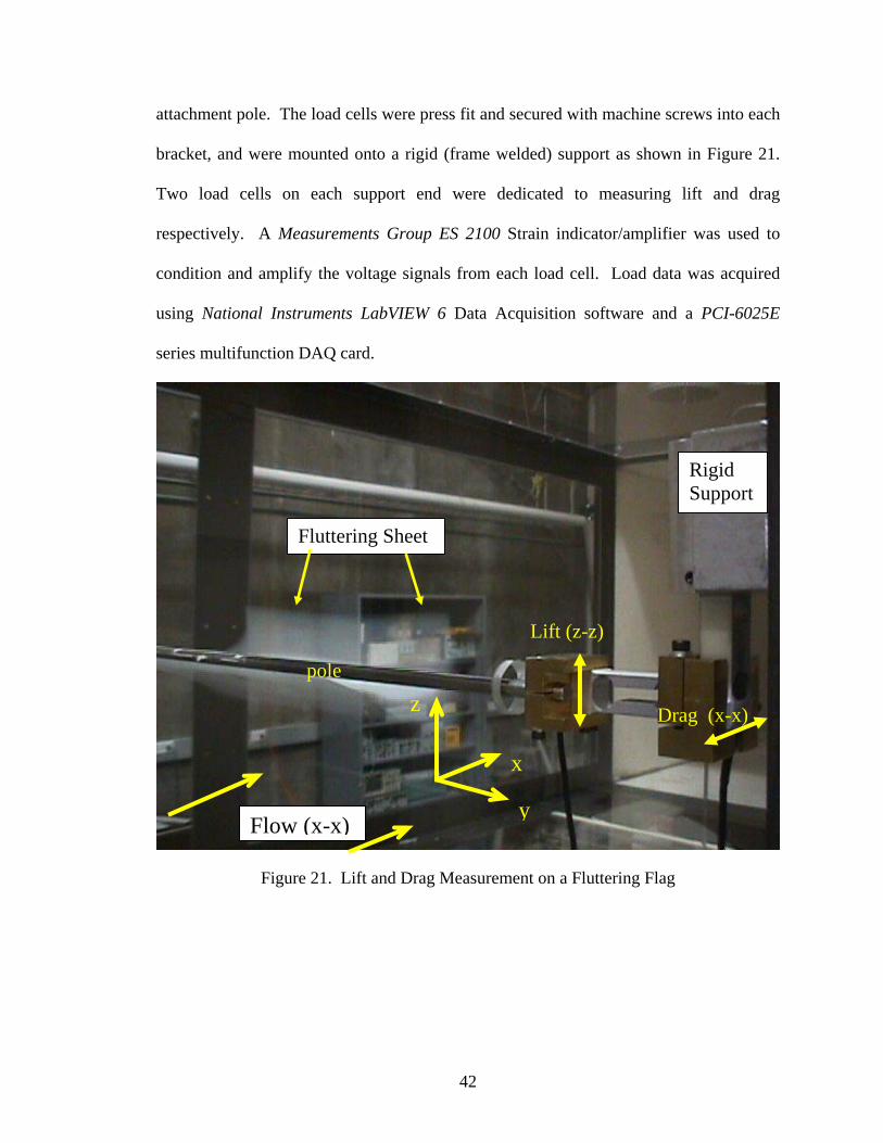
42
attachment pole. The load cells were press fit and secured with machine screws into each
bracket, and were mounted onto a rigid (frame welded) support as shown in Figure 21.
Two load cells on each support end were dedicated to measuring lift and drag
respectively. A Measurements Group ES 2100 Strain indicator/amplifier was used to
condition and amplify the voltage signals from each load cell. Load data was acquired
using National Instruments LabVIEW 6 Data Acquisition software and a PCI-6025E
series multifunction DAQ card.
Figure 21. Lift and Drag Measurement on a Fluttering Flag
Fluttering Sheet
y
x
z Drag (x-x)
Lift (z-z)
Flow (x-x)
Rigid Support
pole
43
Pressure Measurements
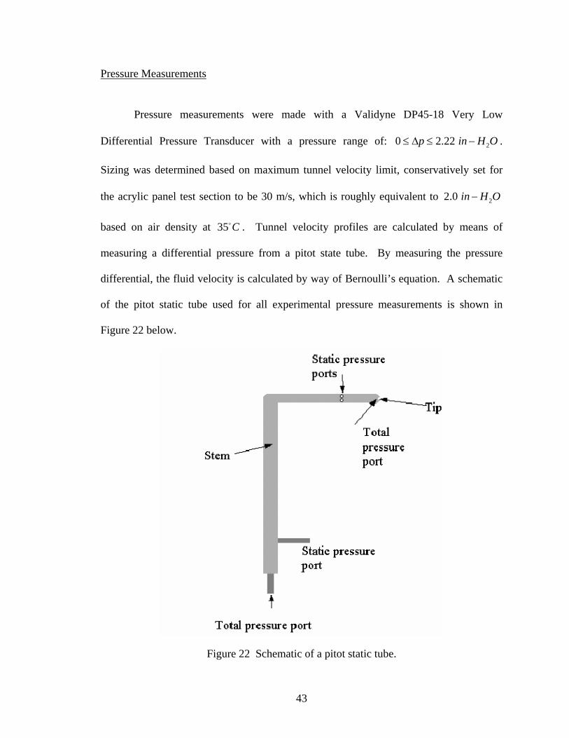
Pressure measurements were made with a Validyne DP45-18 Very Low
Differential Pressure Transducer with a pressure range of: 20 2.22 p in H O≤ Δ ≤ − .
Sizing was determined based on maximum tunnel velocity limit, conservatively set for
the acrylic panel test section to be 30 m/s, which is roughly equivalent to 22.0 in H O−
based on air density at 35 C . Tunnel velocity profiles are calculated by means of
measuring a differential pressure from a pitot state tube. By measuring the pressure
differential, the fluid velocity is calculated by way of Bernoulli’s equation. A schematic
of the pitot static tube used for all experimental pressure measurements is shown in
Figure 22 below.
Figure 22 Schematic of a pitot static tube.

44
The term “pitot static” comes from the fact that the tube requires the measurement of
both static pressure and total pressure for accurate velocity prediction. Total pressure is
also referred to as the “stagnation pressure”, because the fluid velocity is assumed to be
zero at the tip entrance, thus creating the largest pressure. At this point, all of the fluid's
kinetic energy is converted into potential energy, often called pressure energy. Using the
velocity-pressure relationship derived from Bernoulli’s equation in Section 3.1, recall the
total pressure 21 1
12sp p vρ= + can now be applied to compute the free stream fluid
velocity ( )oU .
solving for the free stream velocity:
( )11
2 so
p pv U
ρ−
= =
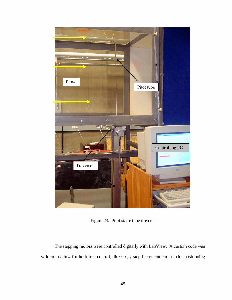
A velocity profile of a center section of the wind tunnel cross-section measuring
26 26 .in× was scanned in 1 in. increments using a bi-directional traverse controlled by
stepping motors. Figure 23 shows the pitot tube mounted within the traverse setup.
45
Figure 23. Pitot static tube traverse
The stepping motors were controlled digitally with LabView. A custom code was
written to allow for both free control, direct x, y step increment control (for positioning
Controlling PC
Flow
Traverse
Pitot tube
46
the pitot tube for general velocity readings) and an automated sweep control, which
performs a sweep in 1 in. increments to the data matrix the user specifies (Appendix E).
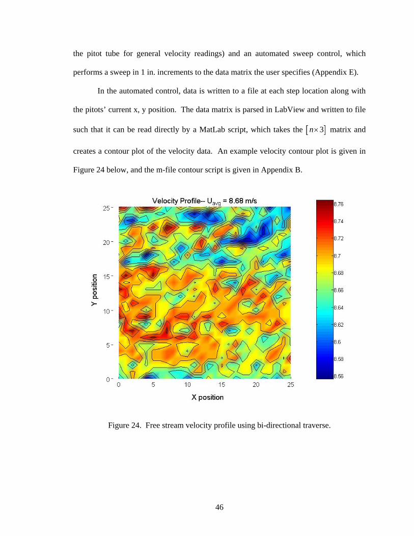
In the automated control, data is written to a file at each step location along with
the pitots’ current x, y position. The data matrix is parsed in LabView and written to file
such that it can be read directly by a MatLab script, which takes the [ ]3n× matrix and
creates a contour plot of the velocity data. An example velocity contour plot is given in
Figure 24 below, and the m-file contour script is given in Appendix B.
Figure 24. Free stream velocity profile using bi-directional traverse.
47
To control the stepping motors, the low current digital pulses from the computer
are fed into a high speed transistor switching circuit. With a 6 Volt power supply
connected to the motors, the transistor served as a switch to ground the coils when the
digital signal from the computer is given to transistor base (power sink). Detailed
schematics of stepping motor operation and circuitry are given in Appendices C-E.
Frequency Measurements
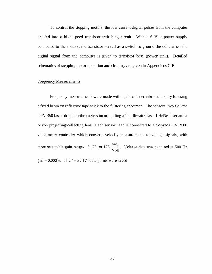
Frequency measurements were made with a pair of laser vibrometers, by focusing
a fixed beam on reflective tape stuck to the fluttering specimen. The sensors: two Polytec
OFV 350 laser–doppler vibrometers incorporating a 1 milliwatt Class II HeNe-laser and a
Nikon projecting/collecting lens. Each sensor head is connected to a Polytec OFV 2600
velocimeter controller which converts velocity measurements to voltage signals, with
three selectable gain ranges: mm
sec5, 25, or 125 Volt
. Voltage data was captured at 500 Hz
( )0.002tΔ = until 152 32,174= data points were saved.
48
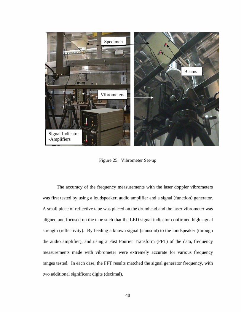
Figure 25. Vibrometer Set-up
The accuracy of the frequency measurements with the laser doppler vibrometers
was first tested by using a loudspeaker, audio amplifier and a signal (function) generator.
A small piece of reflective tape was placed on the drumhead and the laser vibrometer was
aligned and focused on the tape such that the LED signal indicator confirmed high signal
strength (reflectivity). By feeding a known signal (sinusoid) to the loudspeaker (through
the audio amplifier), and using a Fast Fourier Transform (FFT) of the data, frequency
measurements made with vibrometer were extremely accurate for various frequency
ranges tested. In each case, the FFT results matched the signal generator frequency, with
two additional significant digits (decimal).
Specimen
Vibrometers
Signal Indicator -Amplifiers
Beams
49
Frequency measurements were made by placing the reflective tape toward the
center of the sheet, such that the vibrometer laser beam was in constant contact with
reflective tape. Due to the large “whip” action observed at the trailing edge of a
fluttering sheets, the laser beam shot by the vibrometer was unable to stay in constant
contact with the reflective tape. It was hoped that amplitude at the trailing edge (leech)
could be computed with the vibrometers, however the extreme “whip” action at the leech
caused momentary loss of signal. The next subsection discusses the use of a high speed
camera to capture such data.
Traveling Waves
The cross spectrum is a FFT based signal measurement defined as:
( ) ( )( )
2Cross Power Spectrum ( )XY
FFT Y FFT XS f
N
∗•
=
( )( ):
complex conjugate of the FFT of signal x
Number sampled points describing one waveform (x or y)
where
FFT X
N
∗=
=
The cross spectrum is used to compute the phase difference between two signals
of like frequencies. When used with only one measurement signal the cross spectrum is
referred to as a power spectrum, where ( )XXS f is the rms amplitude at an indexed
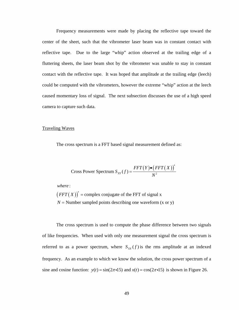
frequency. As an example to which we know the solution, the cross power spectrum of a
sine and cosine function: ( ) sin(2 15) and ( ) cos(2 15)y t x tπ π= =i i is shown in Figure 26.
50
0 5 10 15 20 250
0.01
0.02
0.03
0.04
0.05
0.06
Cross Power Spectrum (Test)
Frequency (Hz)
Am
plitu
de
0 5 10 15 20 25
-80
-60
-40
-20
0
Pha
se (d
eg)
Frequency (Hz)
ω1= 14.9994Hz at φ = -90 deg
Cross Power Signals:y(t) = sin(2π*15) x(t) = cos(2π*15)
Figure 26. Cross spectrum test confirming 90° phase shift of sine and cosine function.
As expected the phase difference between a sine and cosine function is 90 ,
furthermore this test confirms the accuracy and implementation of the Matlab m-file
script that was used to compute all frequency and phase data for flutter experiments. This
script is given in Appendix G. This MatLab script pulls two columns of voltage data
152 2⎡ ⎤⎣ ⎦ from the vibrometers saved in Excel, puts the data through a Hanning window,
computes the FFT for each vector, applies the cross spectrum function, finds the first four
harmonic frequencies, plots the frequency and phase spectrum, and displays the
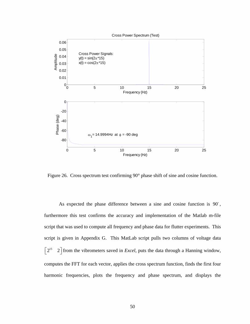
51
fundamental frequency and phase on the plot. An example plot for a flexible sheet with
mass ratio 1.88μ = , is shown in Figure 27.
0 0.5 1 1.5 2 2.5 3 3.5 4 4.5 50
0.002
0.004
0.006
0.008
0.01
0.012Cross Power Spectrum (4.33 m/s) Flag μ=1.88
Am
plitu
de
ω1=3.4332Hz at φ =-7.5209 deg
0 0.5 1 1.5 2 2.5 3 3.5 4 4.5 5
-30
-20
-100
10
20
30
Pha
se (d
eg)
Frequency (Hz)
Figure 27. Cross FFT frequency and phase information for a flexible sheet at 3.43 m/s.
Executing the Matlab cross spectrum script, and zooming in, there is a dominant
“spike” near 3.5 Hz. This spike is a quantitative measure of the power, and hence the
relative contribution to the entire frequency spectrum. We find the exact location of the
fundamental frequency to occur at 3.43 Hz . Utilizing the same index to find frequency,
the corresponding phase angle is 7.52− . This approach is continued for increasing

52
velocities to form plots of frequency and phase vs. velocity. These results will be
displayed and discussed in Section 4.4.
Mode Shape Measurements
A model XS42GB-MONO high speed digital camera from Integrated Design
Tools, Inc. (IDT) was used to capture frame by frame deflection profiles at 500 Hz
( )0.002 secondstΔ = . The camera was set approximately four feet from the specimen
and was pointed perpendicular with the edge of the fluttering specimen as shown in
Figure 28. Because of the large amplitude deflections and curling at the leech, measuring
high speed images (pixel correlation) is thought to be the only accurate method to
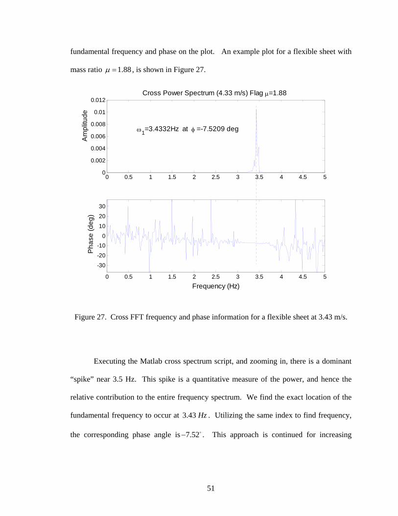
compute the amplitude at the leech.
53
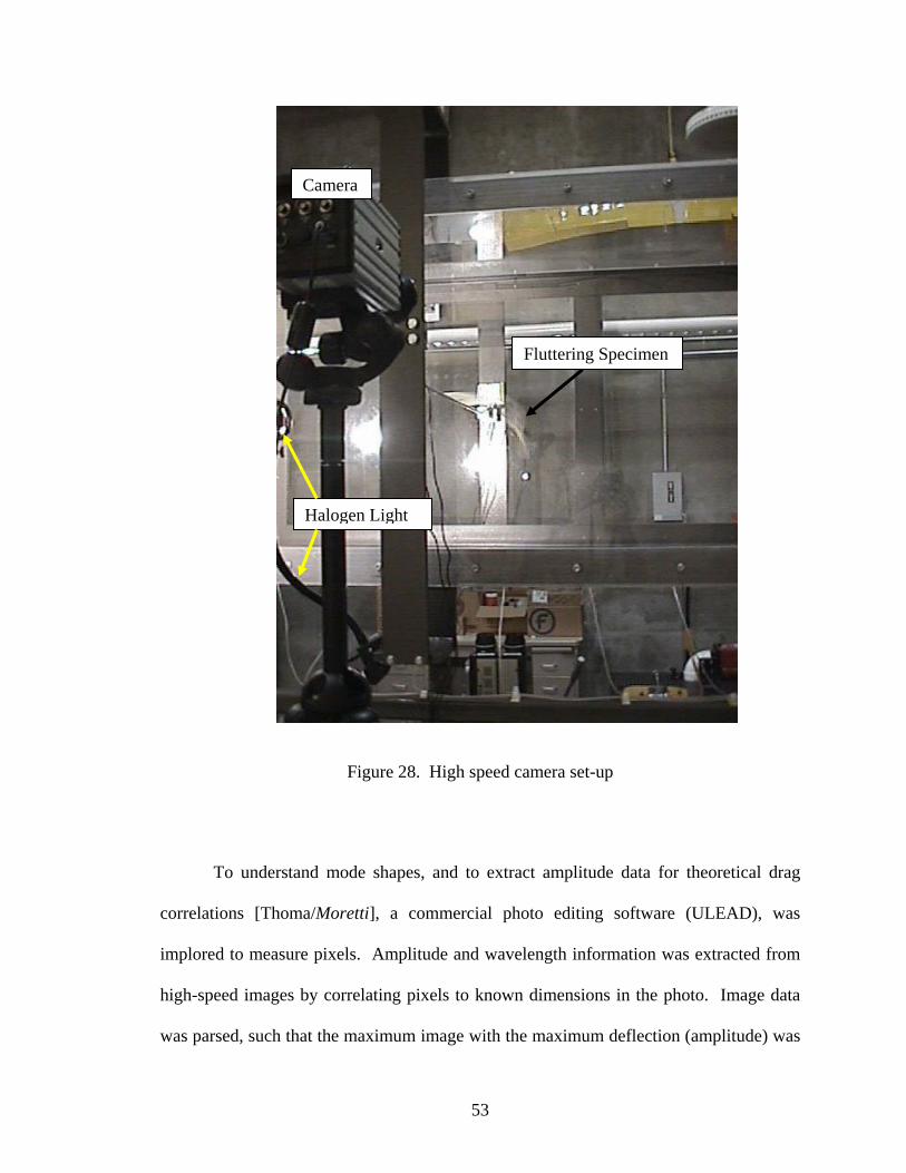
Figure 28. High speed camera set-up
To understand mode shapes, and to extract amplitude data for theoretical drag
correlations [Thoma/Moretti], a commercial photo editing software (ULEAD), was
implored to measure pixels. Amplitude and wavelength information was extracted from
high-speed images by correlating pixels to known dimensions in the photo. Image data
was parsed, such that the maximum image with the maximum deflection (amplitude) was
Fluttering Specimen
Halogen Light
Camera
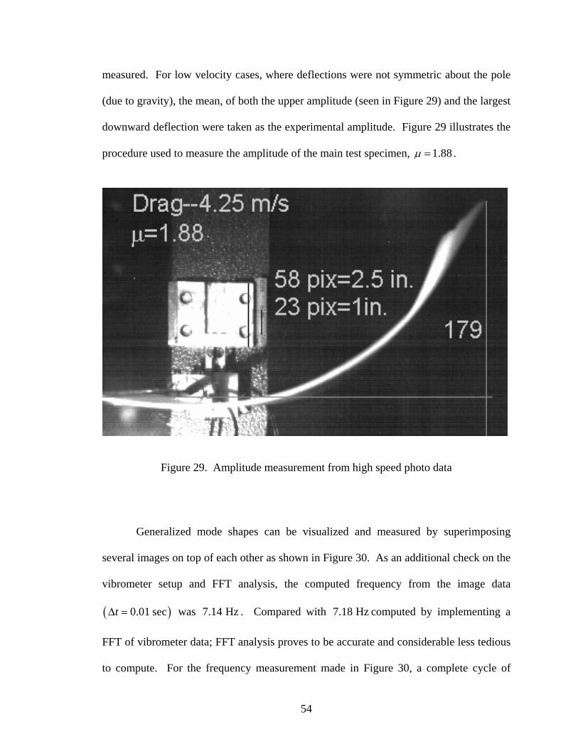
54
measured. For low velocity cases, where deflections were not symmetric about the pole
(due to gravity), the mean, of both the upper amplitude (seen in Figure 29) and the largest
downward deflection were taken as the experimental amplitude. Figure 29 illustrates the
procedure used to measure the amplitude of the main test specimen, 1.88μ = .
Figure 29. Amplitude measurement from high speed photo data
Generalized mode shapes can be visualized and measured by superimposing
several images on top of each other as shown in Figure 30. As an additional check on the
vibrometer setup and FFT analysis, the computed frequency from the image data
( )0.01 sectΔ = was 7.14 Hz . Compared with 7.18 Hz computed by implementing a
FFT of vibrometer data; FFT analysis proves to be accurate and considerable less tedious
to compute. For the frequency measurement made in Figure 30, a complete cycle of
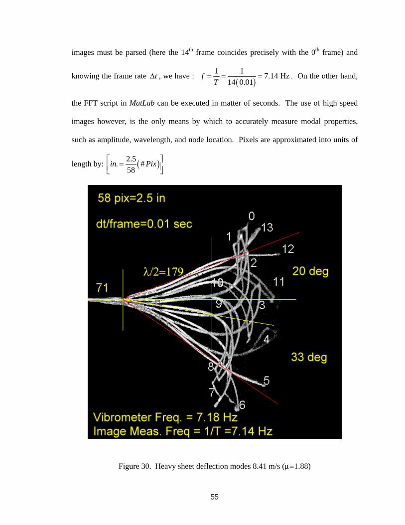
55
images must be parsed (here the 14th frame coincides precisely with the 0th frame) and
knowing the frame rate tΔ , we have : ( )
1 1 7.14 Hz14 0.01
fT
= = = . On the other hand,
the FFT script in MatLab can be executed in matter of seconds. The use of high speed
images however, is the only means by which to accurately measure modal properties,
such as amplitude, wavelength, and node location. Pixels are approximated into units of
length by: ( )2.5. #58
in Pix⎡ ⎤=⎢ ⎥⎣ ⎦
Figure 30. Heavy sheet deflection modes 8.41 m/s (μ=1.88)

56
4.2 Experimental Procedure
The quantities measured and/or computed in this experiment were DF , LF ,
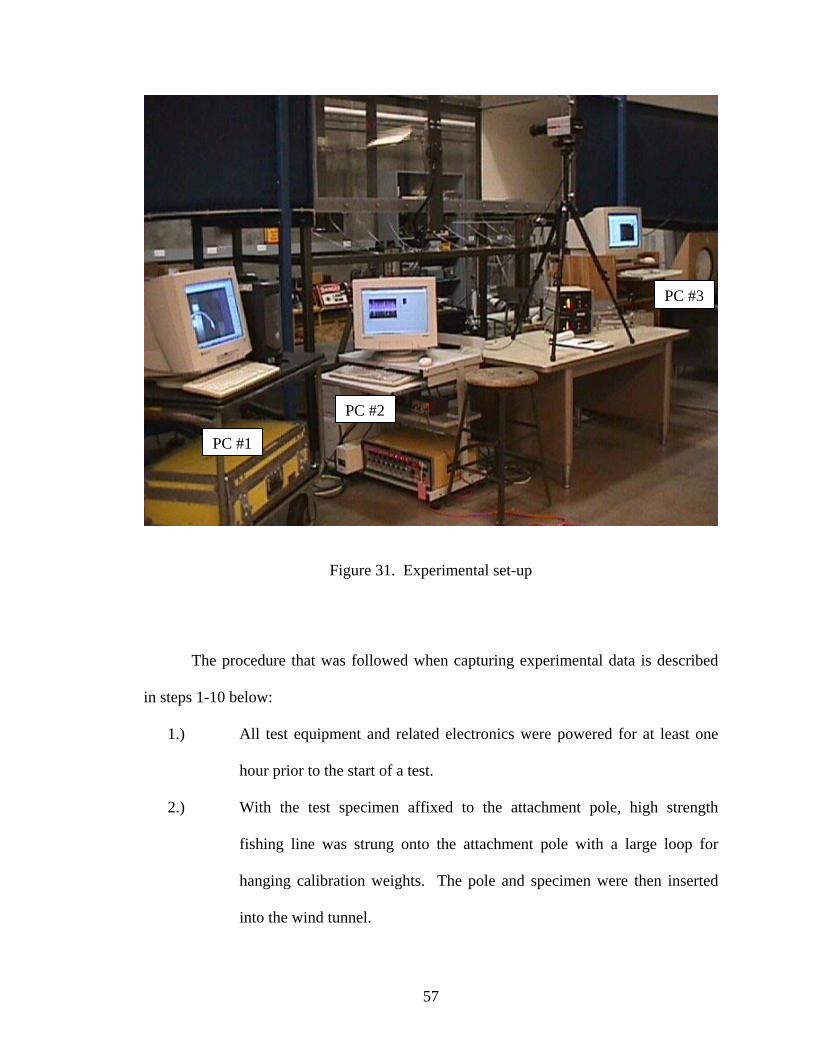
( ) p vΔ , Hzf , roomT , and high speed image deflections. Three independent personal
computers were used to gather the experimental data as shown in Figure 31. PC #1 was
used to capture high speed deflection images, PC #2 was used to capture drag data from
the four load cells and pressure data ( )pΔ from the pitot-static tube, and PC #3 was used
to control the pitot traverse, record pressure data during cross-section sweeps (velocity
profiles), and record frequency signals from the two vibrometers. The pressure
transducer signal was split, and sent to PC #2 and PC #3 for simultaneous velocity
correlations between experimental variables. Each pressure signal was independently
calibrated to account for lead wire resistance.
57
Figure 31. Experimental set-up
The procedure that was followed when capturing experimental data is described
in steps 1-10 below:
1.) All test equipment and related electronics were powered for at least one
hour prior to the start of a test.
2.) With the test specimen affixed to the attachment pole, high strength
fishing line was strung onto the attachment pole with a large loop for
hanging calibration weights. The pole and specimen were then inserted
into the wind tunnel.
PC #1
PC #2
PC #3
58
3.) With specimen in place, the wind tunnel was slowly ramped to a
maximum test velocity, where the specimen either exhibited three
dimensional (and/or irregular) deflections, or experienced especially
violent oscillations close to exceeding load cell capacities. At this critical
velocity, drag data was recorded to check signal strength and/or saturation.
The signal conditioner gain (amplification) was then adjusted such that the
output was very close to, but less than the saturation voltage of the AD
card. The tunnel was then turned off, and the drag channels were adjusted
to zero output. The tunnel was then ramped up again to the critical
velocity to check saturation. This procedure was repeated until a
satisfactory nulling was seen at no wind velocity, and a maximum output
(under AD saturation) was seen at the critical velocity. Gain and nulling
knobs were then locked in position.
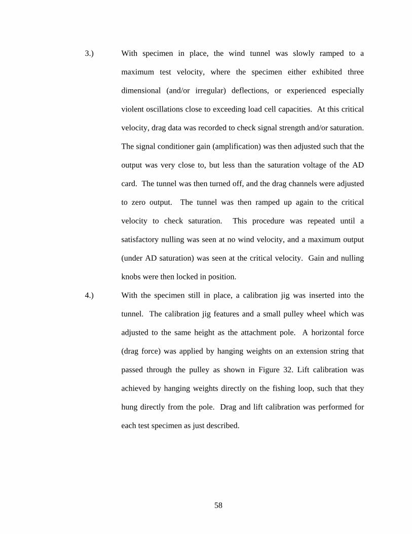
4.) With the specimen still in place, a calibration jig was inserted into the
tunnel. The calibration jig features and a small pulley wheel which was
adjusted to the same height as the attachment pole. A horizontal force
(drag force) was applied by hanging weights on an extension string that
passed through the pulley as shown in Figure 32. Lift calibration was
achieved by hanging weights directly on the fishing loop, such that they
hung directly from the pole. Drag and lift calibration was performed for
each test specimen as just described.
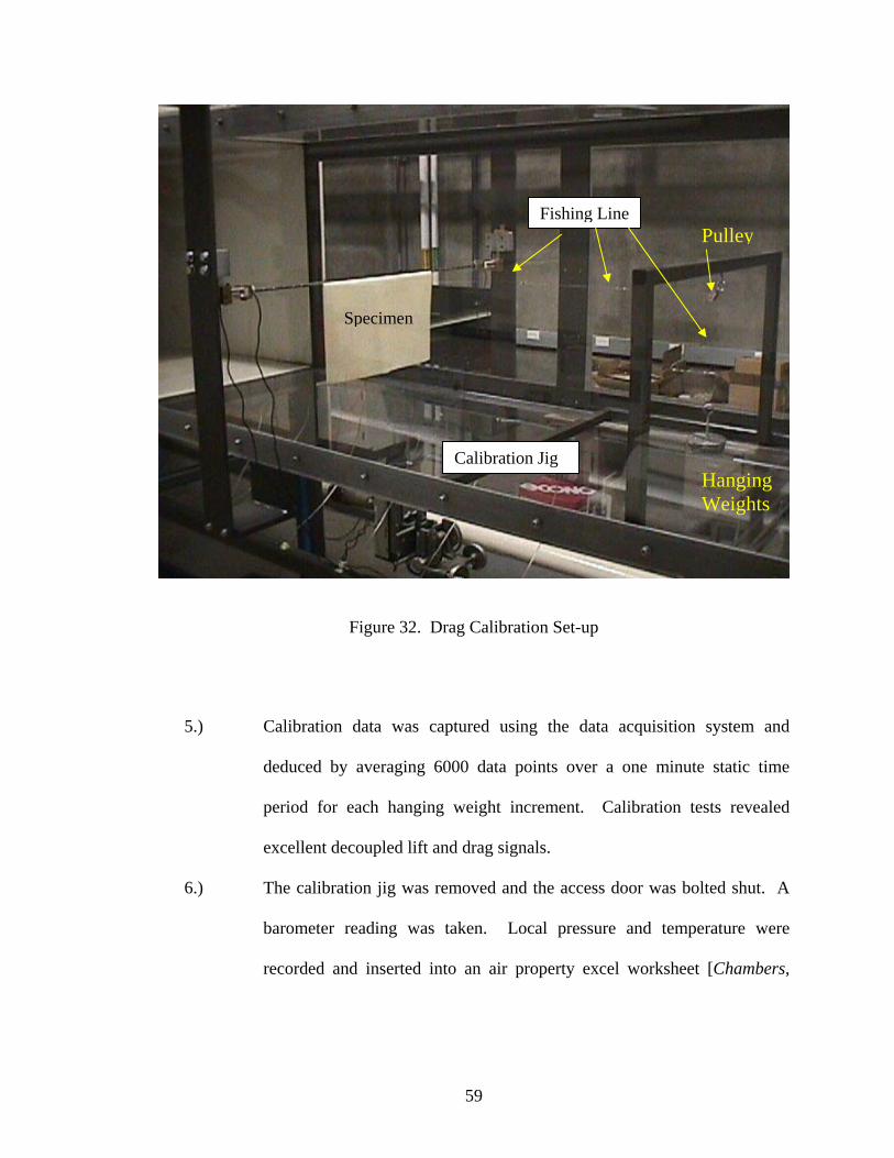
59
Figure 32. Drag Calibration Set-up
5.) Calibration data was captured using the data acquisition system and
deduced by averaging 6000 data points over a one minute static time
period for each hanging weight increment. Calibration tests revealed
excellent decoupled lift and drag signals.
6.) The calibration jig was removed and the access door was bolted shut. A
barometer reading was taken. Local pressure and temperature were
recorded and inserted into an air property excel worksheet [Chambers,
Calibration Jig
Specimen
Hanging Weights
Fishing Line Pulley

60
Appendix I], and then saved as a copy into a newly created test case
folder.
7.) The wind tunnel was ramped to the critical wind velocity in increments of
20.02 in H O− , by monitoring a manometer hooked in parallel with the
pitot pressure transducer. Drag data was sampled every 10 ms for one
minute. Once the drag PC was initiated, frequency data collection (PC #3)
was started. Data was collected at 500 Hz ( )2 samplingt msΔ = until
152 32,768= data points were captured. After initiating the frequency
measurement, the high speed camera was used to capture images at 500
Hz ( )2 samplingt msΔ = . Images were recorded for 5 seconds and stored
onto the cameras internal memory. Playing back the images, two
complete cycles of oscillation were saved to disk to reduce the file size.
8.) The tunnel speed was increasing by 20.02 p in H OΔ = − , and step 7 was
repeated.
9.) After the critical velocity data was recorded, the tunnel was ramped down
and turned off. At no wind velocity, load cell data was captured again to
ensure negligible drift.
10.) The barometer was read again. Local pressure and temperature were
inserted into the air calculator and saved into the test folder. The density
computed by the sheet before and after the test was averaged and used in
velocity calculations.

61
4.3 Estimation of the Uncertainty of Drag Force
The experimental drag and lift forces were measured with four identical load cells
with the performance specification given by the manufacture. Important specifications
are summarized in Table 1 below.
Performance Property Specification
Capacity 1.0 2.21 Kgf lbf=
Rated Output mv0.933 V
Nonlinearity 0.02% FS
Excitation Voltage 10 V DC
Table 1. Transducer Techniques LSP-1 Load Cell Specifications
To find the uncertainty of the drag force, the propagation of uncertainty approach
is implored, as described by Holman (1995). The most insightful drag case (and heavily
studied) was for a flexible sheet with a mass ratio 1.88μ = . The material was a heavy
“leather” fabric, which exhibited consistent (steady) 2-D deflections for a wide range of
wind velocities. To compute the uncertainty of drag force, the calibration equation
describing the output force as a function of the transducer output voltage is given in
equation (4-3.1) below.
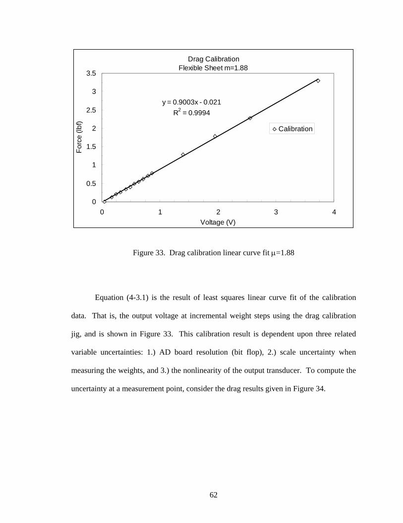
( )0.9003 V 0.021DF = − (4-3.1)
62
Drag CalibrationFlexible Sheet m=1.88
y = 0.9003x - 0.021R2 = 0.9994
0
0.5
1
1.5
2
2.5
3
3.5
0 1 2 3 4Voltage (V)
Forc
e (lb
f)
Calibration
Figure 33. Drag calibration linear curve fit μ=1.88
Equation (4-3.1) is the result of least squares linear curve fit of the calibration
data. That is, the output voltage at incremental weight steps using the drag calibration
jig, and is shown in Figure 33. This calibration result is dependent upon three related
variable uncertainties: 1.) AD board resolution (bit flop), 2.) scale uncertainty when
measuring the weights, and 3.) the nonlinearity of the output transducer. To compute the
uncertainty at a measurement point, consider the drag results given in Figure 34.
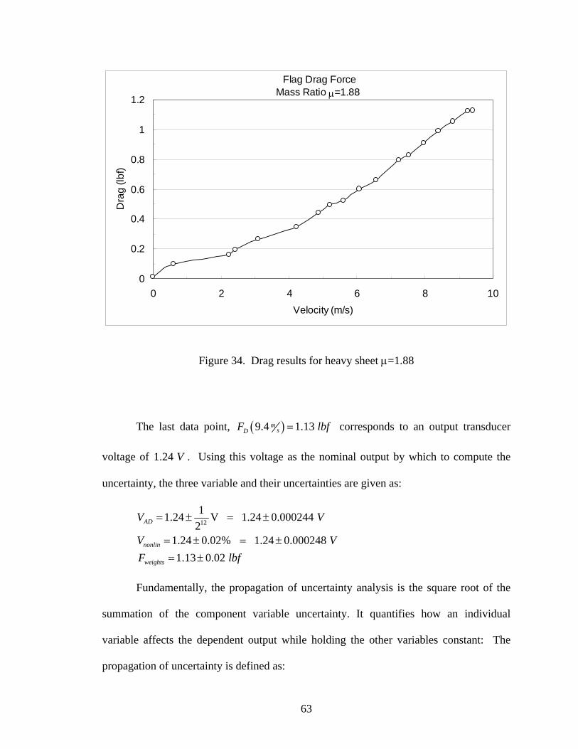
63
Flag Drag Force Mass Ratio μ=1.88
0
0.2
0.4
0.6
0.8
1
1.2
0 2 4 6 8 10Velocity (m/s)
Dra
g (lb
f)
Figure 34. Drag results for heavy sheet μ=1.88
The last data point, ( )9.4 1.13 msDF lbf= corresponds to an output transducer
voltage of 1.24 V . Using this voltage as the nominal output by which to compute the
uncertainty, the three variable and their uncertainties are given as:
12
11.24 V 1.24 0.000244 2
1.24 0.02% 1.24 0.000248 1.13 0.02
AD
nonlin
weights
V V
V VF lbf
= ± = ±
= ± = ±= ±
Fundamentally, the propagation of uncertainty analysis is the square root of the
summation of the component variable uncertainty. It quantifies how an individual
variable affects the dependent output while holding the other variables constant: The
propagation of uncertainty is defined as:
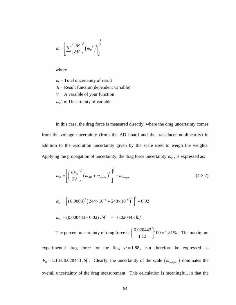
64
( )1
2 22
VRV
ω ω ∗⎡ ⎤∂⎛ ⎞= ⎢ ⎥⎜ ⎟∂⎝ ⎠⎢ ⎥⎣ ⎦∑
where
Total uncertainty of resultResult function(dependent variable)A varaible of your function
Uncertainty of variableV
RV
ω
ω ∗
===
=
In this case, the drag force is measured directly, where the drag uncertainty comes
from the voltage uncertainty (from the AD board and the transducer nonlinearity) in
addition to the resolution uncertainty given by the scale used to weigh the weights.
Applying the propagation of uncertainty, the drag force uncertainty Fω , is expressed as:
( )1
2 22D
F AD nonlin weightsFV
ω ω ω ω⎡ ⎤∂⎛ ⎞= + +⎢ ⎥⎜ ⎟∂⎝ ⎠⎢ ⎥⎣ ⎦
(4-3.2)
( ) ( )1222 6 60.9003 244 10 248 10 0.02
(0.000443 0.02) 0.020443
F
F lbf lbf
ω
ω
− −⎡ ⎤= × + × +⎢ ⎥⎣ ⎦
= + =
The percent uncertainty of drag force is 0.020443 100 1.81%1.13
⎛ ⎞ =⎜ ⎟⎝ ⎠
. The maximum
experimental drag force for the flag 1.88μ = , can therefore be expressed as
1.13 0.020443 DF lbf= ± . Clearly, the uncertainty of the scale ( )weightsω dominates the
overall uncertainty of the drag measurement. This calculation is meaningful, in that the

65
“weak link” in establishing measurement confidence, is not in the transducer, but rather
the instrument that was used to calibrate the transducer. Measurement confidence can
therefore be increased by using a scale with higher resolution. A similar uncertainty
analysis is performed for pitot tube pressure measurement in Appendix F.
4.4 Experimental Results
Light-Weight Flexible Sheet μ =0.704
A light weight and flexible sheet (lighter than a bed sheet) was first tested. Light
weight materials were found to exhibit flutter oscillations at low wind velocities and
flutter consistently for only a small range of wind velocities. When the wind speed was
increased beyond a critical stability velocity, the flag would oscillate in very
unpredictable / sporadic 3-D deformations. In such a situation, the flutter frequency and
drag force was seen to drop; as a consequence of periods of momentary fold over. For
the first drag experiment, frequency data was recorded and processed immediately by
utilizing a LabView auto-spectrum subvi (Appendix H). Figure 35 illustrates the sudden
flutter onset and “falloff”, over a very small velocity range.
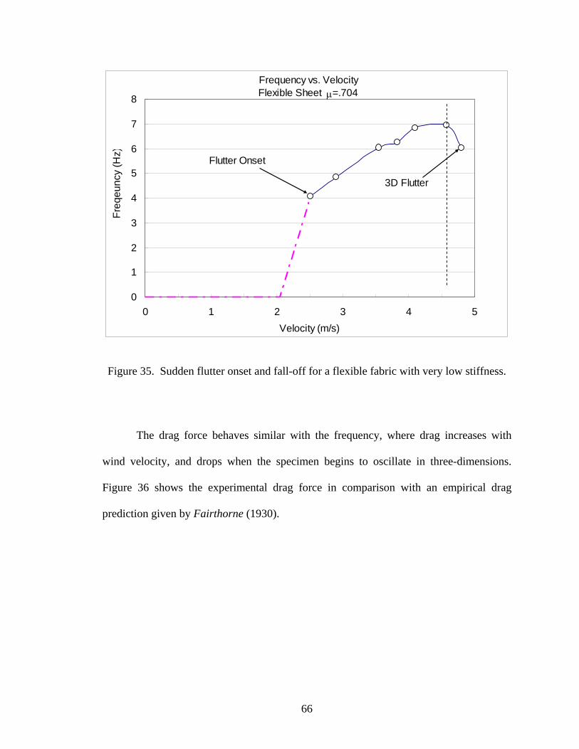
66
Frequency vs. VelocityFlexible Sheet μ=.704
0
1
2
3
4
5
6
7
8
0 1 2 3 4 5Velocity (m/s)
Freq
eunc
y (H
z)
Flutter Onset
3D Flutter
Figure 35. Sudden flutter onset and fall-off for a flexible fabric with very low stiffness.
The drag force behaves similar with the frequency, where drag increases with
wind velocity, and drops when the specimen begins to oscillate in three-dimensions.
Figure 36 shows the experimental drag force in comparison with an empirical drag
prediction given by Fairthorne (1930).
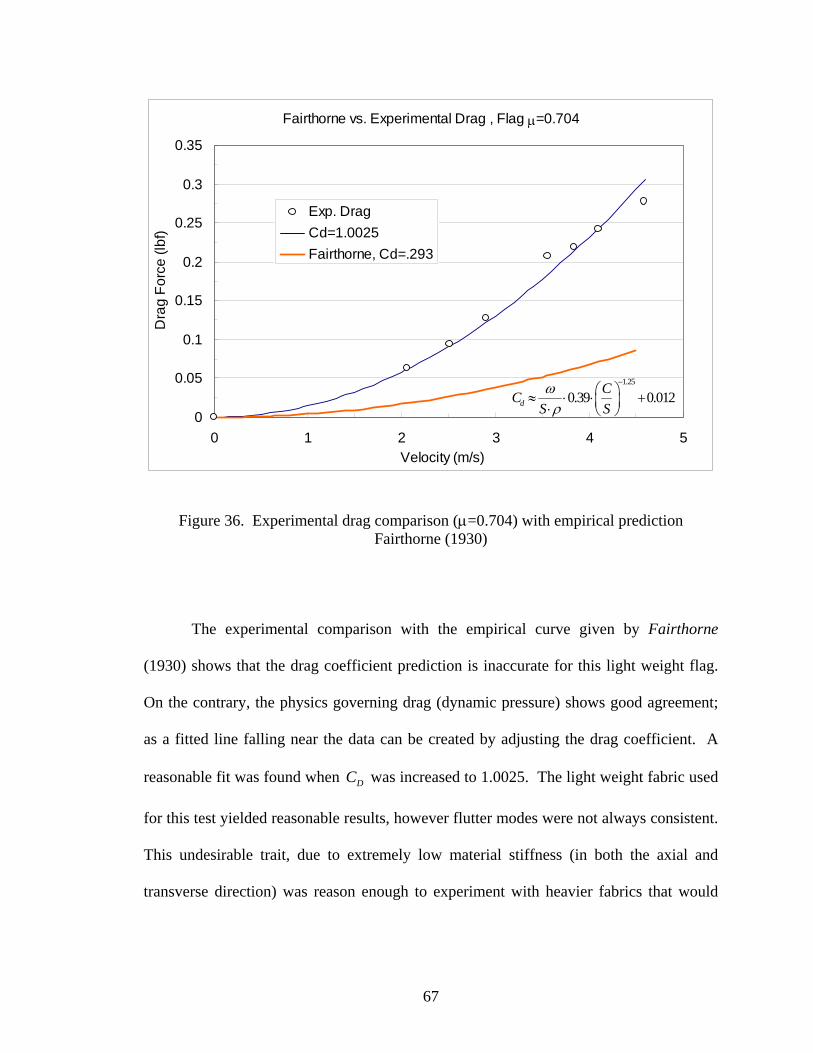
67
Fairthorne vs. Experimental Drag , Flag μ=0.704
0
0.05
0.1
0.15
0.2
0.25
0.3
0.35
0 1 2 3 4 5Velocity (m/s)
Dra
g Fo
rce
(lbf)
Exp. DragCd=1.0025Fairthorne, Cd=.293
1.25
0.39 0.012dCC
S Sω
ρ
−⎛ ⎞≈ ⋅ ⋅ +⎜ ⎟⋅ ⎝ ⎠
Figure 36. Experimental drag comparison (μ=0.704) with empirical prediction Fairthorne (1930)
The experimental comparison with the empirical curve given by Fairthorne
(1930) shows that the drag coefficient prediction is inaccurate for this light weight flag.
On the contrary, the physics governing drag (dynamic pressure) shows good agreement;
as a fitted line falling near the data can be created by adjusting the drag coefficient. A
reasonable fit was found when DC was increased to 1.0025. The light weight fabric used
for this test yielded reasonable results, however flutter modes were not always consistent.
This undesirable trait, due to extremely low material stiffness (in both the axial and
transverse direction) was reason enough to experiment with heavier fabrics that would
68
demonstrate consistent 2-D deflections, allowing ease of study and comparison with
simplified 2-D theories.
Semi-Rigid Cooking Board μ =1.74
A flexible cutting board (cooking board) was tested as an opposite extreme to the
last material ( )0.704μ = , yet was still capable of flutter. It was flexible enough to bend
under its own weight when supported like a flag, but considerable stiffer than the other
fabric cases.
Figure 37. Semi-Rigid Cooking Board
Flutter modes of the cutting board were similar to flexible sheets, however the
board did not experience extreme curling at the leech when it reached its maximum
potential. Figure 38 shows the fundamental frequency and phase angle for the cooking
board. Note that the first flutter data point, was just before symmetric (regular)
oscillations, and represents the frequency and phase when the board was just beginning to
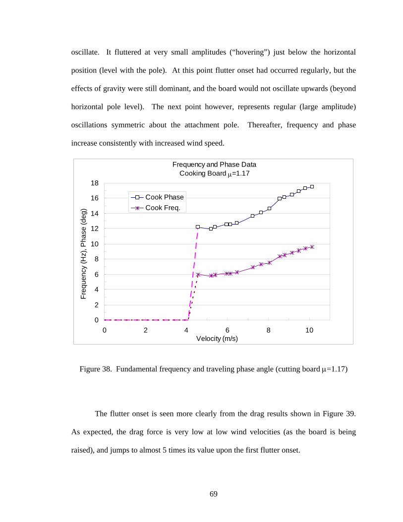
69
oscillate. It fluttered at very small amplitudes (“hovering”) just below the horizontal
position (level with the pole). At this point flutter onset had occurred regularly, but the
effects of gravity were still dominant, and the board would not oscillate upwards (beyond
horizontal pole level). The next point however, represents regular (large amplitude)
oscillations symmetric about the attachment pole. Thereafter, frequency and phase
increase consistently with increased wind speed.
Frequency and Phase DataCooking Board μ=1.17
0
2
4
6
8
10
12
14
16
18
0 2 4 6 8 10Velocity (m/s)
Freq
uenc
y (H
z), P
hase
(deg
)
Cook PhaseCook Freq.
Figure 38. Fundamental frequency and traveling phase angle (cutting board μ=1.17)
The flutter onset is seen more clearly from the drag results shown in Figure 39.
As expected, the drag force is very low at low wind velocities (as the board is being
raised), and jumps to almost 5 times its value upon the first flutter onset.
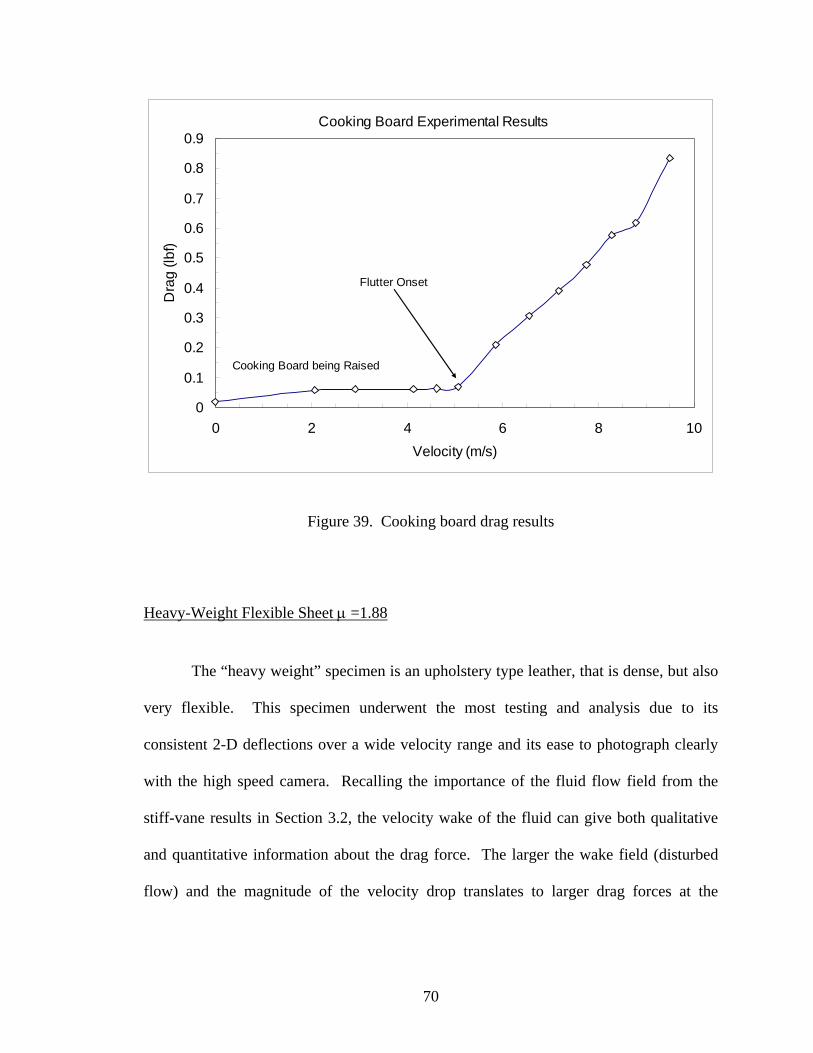
70
Cooking Board Experimental Results
0
0.1
0.2
0.3
0.4
0.5
0.6
0.7
0.8
0.9
0 2 4 6 8 10Velocity (m/s)
Dra
g (lb
f)
Flutter Onset
Cooking Board being Raised
Figure 39. Cooking board drag results
Heavy-Weight Flexible Sheet μ =1.88
The “heavy weight” specimen is an upholstery type leather, that is dense, but also
very flexible. This specimen underwent the most testing and analysis due to its
consistent 2-D deflections over a wide velocity range and its ease to photograph clearly
with the high speed camera. Recalling the importance of the fluid flow field from the
stiff-vane results in Section 3.2, the velocity wake of the fluid can give both qualitative
and quantitative information about the drag force. The larger the wake field (disturbed
flow) and the magnitude of the velocity drop translates to larger drag forces at the
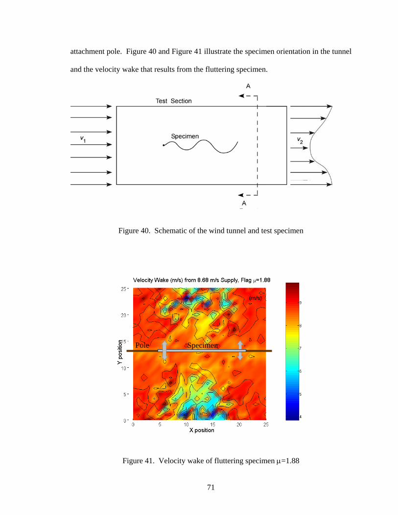
71
attachment pole. Figure 40 and Figure 41 illustrate the specimen orientation in the tunnel
and the velocity wake that results from the fluttering specimen.
Figure 40. Schematic of the wind tunnel and test specimen
Figure 41. Velocity wake of fluttering specimen μ=1.88
Pole Specimen
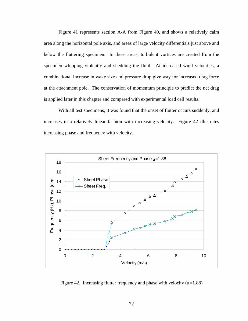
72
Figure 41 represents section A-A from Figure 40, and shows a relatively calm
area along the horizontal pole axis, and areas of large velocity differentials just above and
below the fluttering specimen. In these areas, turbulent vortices are created from the
specimen whipping violently and shedding the fluid. At increased wind velocities, a
combinational increase in wake size and pressure drop give way for increased drag force
at the attachment pole. The conservation of momentum principle to predict the net drag
is applied later in this chapter and compared with experimental load cell results.
With all test specimens, it was found that the onset of flutter occurs suddenly, and
increases in a relatively linear fashion with increasing velocity. Figure 42 illustrates
increasing phase and frequency with velocity.
Sheet Frequency and Phase μ=1.88
0
2
4
6
8
10
12
14
16
18
0 2 4 6 8 10Velocity (m/s)
Freq
uenc
y (H
z), P
hase
(deg
) Sheet PhaseSheet Freq.
Figure 42. Increasing flutter frequency and phase with velocity (μ=1.88)

73
Recalling the frequency measurement section, 4.1, the presence of a phase
difference between the two vibrometer signals proves that the waving deflection modes
are traveling. This test was stopped before 10 m/s due to the violent oscillations (still 2-
D) and increased drag force, which was close to exceeding load cell capacities.
Looking closer at the deflection profiles at a wind speed of 8.84 m/s, Figure 43.
shows two superimposed images that are separated by 2 cycles.
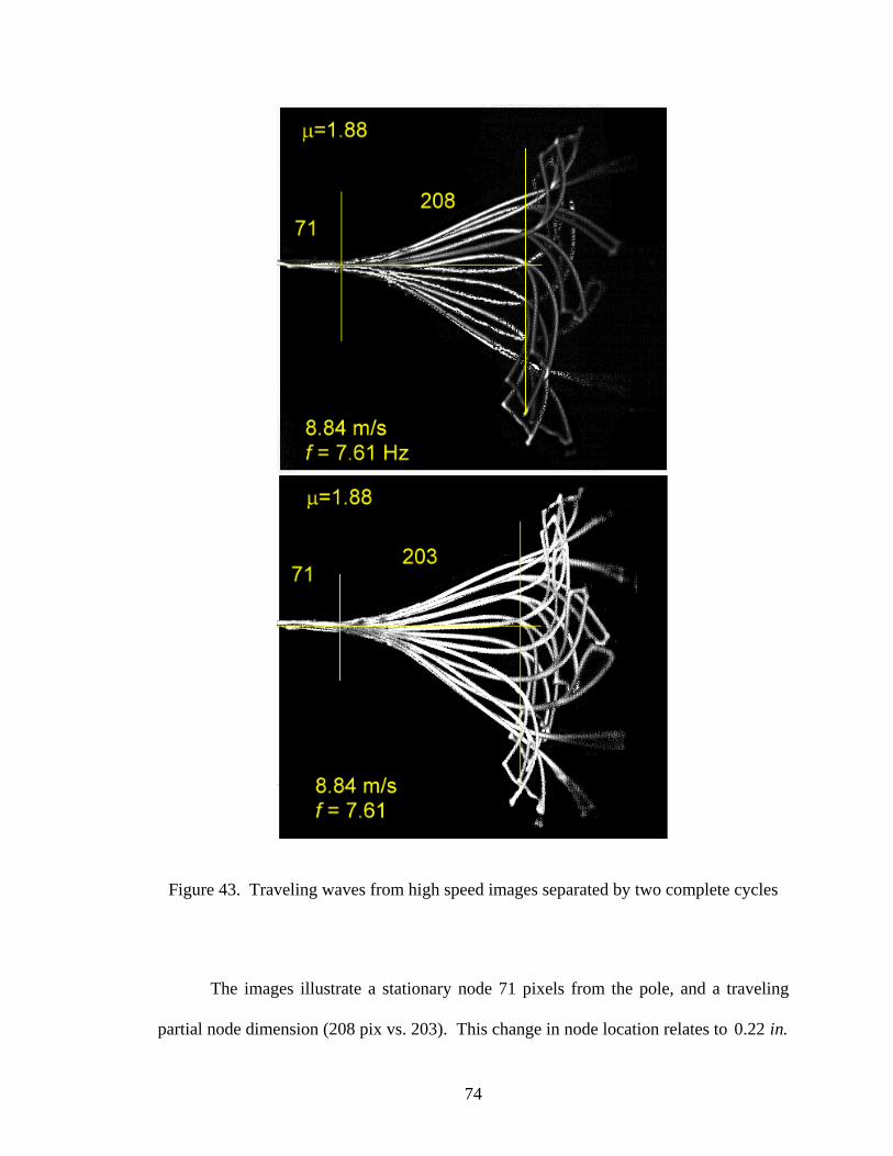
74
Figure 43. Traveling waves from high speed images separated by two complete cycles
The images illustrate a stationary node 71 pixels from the pole, and a traveling
partial node dimension (208 pix vs. 203). This change in node location relates to 0.22 .in
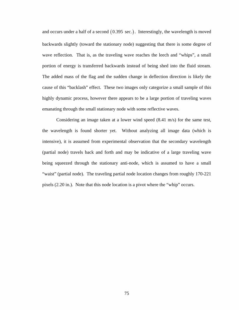
75
and occurs under a half of a second ( )0.395 sec. . Interestingly, the wavelength is moved
backwards slightly (toward the stationary node) suggesting that there is some degree of
wave reflection. That is, as the traveling wave reaches the leech and “whips”, a small
portion of energy is transferred backwards instead of being shed into the fluid stream.
The added mass of the flag and the sudden change in deflection direction is likely the
cause of this “backlash” effect. These two images only categorize a small sample of this
highly dynamic process, however there appears to be a large portion of traveling waves
emanating through the small stationary node with some reflective waves.
Considering an image taken at a lower wind speed (8.41 m/s) for the same test,
the wavelength is found shorter yet. Without analyzing all image data (which is
intensive), it is assumed from experimental observation that the secondary wavelength
(partial node) travels back and forth and may be indicative of a large traveling wave
being squeezed through the stationary anti-node, which is assumed to have a small
“waist” (partial node). The traveling partial node location changes from roughly 170-221
pixels (2.20 in.). Note that this node location is a pivot where the “whip” occurs.
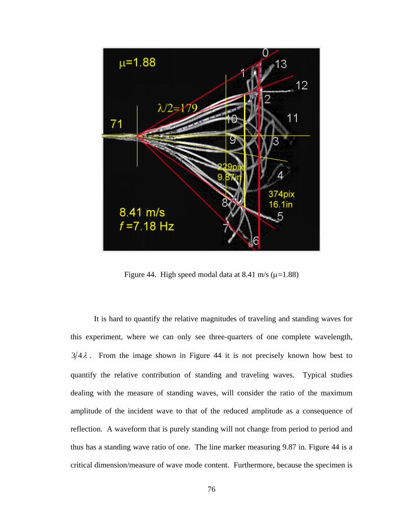
76
Figure 44. High speed modal data at 8.41 m/s (μ=1.88)
It is hard to quantify the relative magnitudes of traveling and standing waves for
this experiment, where we can only see three-quarters of one complete wavelength,
3 4λ . From the image shown in Figure 44 it is not precisely known how best to
quantify the relative contribution of standing and traveling waves. Typical studies
dealing with the measure of standing waves, will consider the ratio of the maximum
amplitude of the incident wave to that of the reduced amplitude as a consequence of
reflection. A waveform that is purely standing will not change from period to period and
thus has a standing wave ratio of one. The line marker measuring 9.87 in. Figure 44 is a
critical dimension/measure of wave mode content. Furthermore, because the specimen is
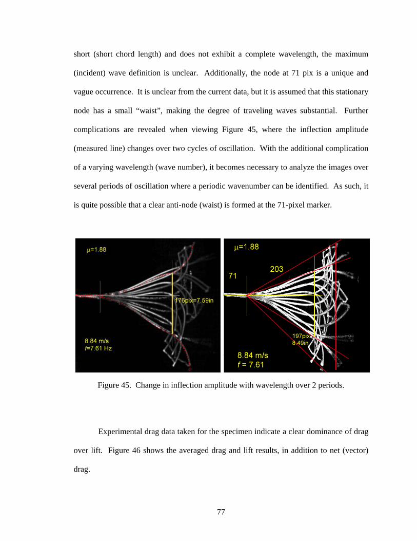
77
short (short chord length) and does not exhibit a complete wavelength, the maximum
(incident) wave definition is unclear. Additionally, the node at 71 pix is a unique and
vague occurrence. It is unclear from the current data, but it is assumed that this stationary
node has a small “waist”, making the degree of traveling waves substantial. Further
complications are revealed when viewing Figure 45, where the inflection amplitude
(measured line) changes over two cycles of oscillation. With the additional complication
of a varying wavelength (wave number), it becomes necessary to analyze the images over
several periods of oscillation where a periodic wavenumber can be identified. As such, it
is quite possible that a clear anti-node (waist) is formed at the 71-pixel marker.
Figure 45. Change in inflection amplitude with wavelength over 2 periods.
Experimental drag data taken for the specimen indicate a clear dominance of drag
over lift. Figure 46 shows the averaged drag and lift results, in addition to net (vector)
drag.
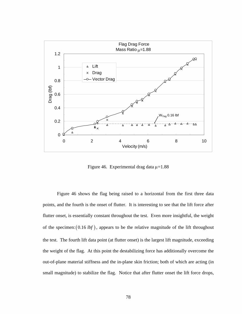
78
Flag Drag Force Mass Ratio μ=1.88
0
0.2
0.4
0.6
0.8
1
1.2
0 2 4 6 8 10Velocity (m/s)
Dra
g (lb
f)
LiftDragVector Drag
Wf lag 0.16 lbf
Figure 46. Experimental drag data μ=1.88
Figure 46 shows the flag being raised to a horizontal from the first three data
points, and the fourth is the onset of flutter. It is interesting to see that the lift force after
flutter onset, is essentially constant throughout the test. Even more insightful, the weight
of the specimen: ( )0.16 lbf , appears to be the relative magnitude of the lift throughout
the test. The fourth lift data point (at flutter onset) is the largest lift magnitude, exceeding
the weight of the flag. At this point the destabilizing force has additionally overcome the
out-of-plane material stiffness and the in-plane skin friction; both of which are acting (in
small magnitude) to stabilize the flag. Notice that after flutter onset the lift force drops,
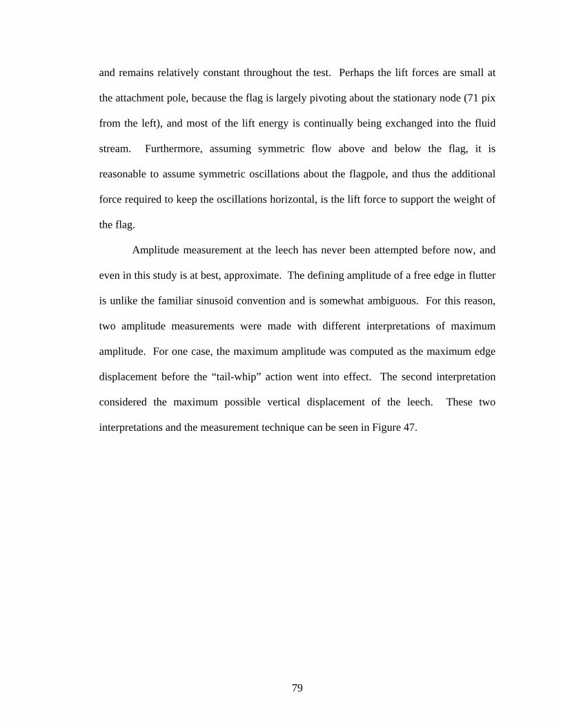
79
and remains relatively constant throughout the test. Perhaps the lift forces are small at
the attachment pole, because the flag is largely pivoting about the stationary node (71 pix
from the left), and most of the lift energy is continually being exchanged into the fluid
stream. Furthermore, assuming symmetric flow above and below the flag, it is
reasonable to assume symmetric oscillations about the flagpole, and thus the additional
force required to keep the oscillations horizontal, is the lift force to support the weight of
the flag.
Amplitude measurement at the leech has never been attempted before now, and
even in this study is at best, approximate. The defining amplitude of a free edge in flutter
is unlike the familiar sinusoid convention and is somewhat ambiguous. For this reason,
two amplitude measurements were made with different interpretations of maximum
amplitude. For one case, the maximum amplitude was computed as the maximum edge
displacement before the “tail-whip” action went into effect. The second interpretation
considered the maximum possible vertical displacement of the leech. These two
interpretations and the measurement technique can be seen in Figure 47.
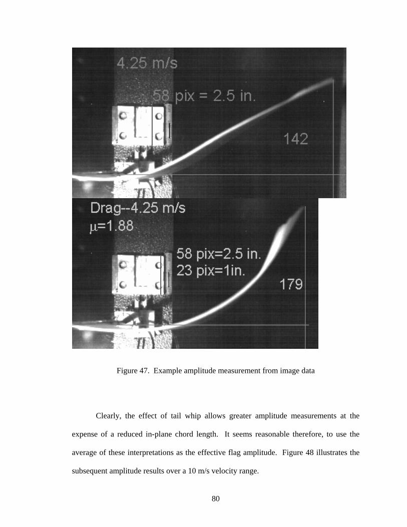
80
Figure 47. Example amplitude measurement from image data
Clearly, the effect of tail whip allows greater amplitude measurements at the
expense of a reduced in-plane chord length. It seems reasonable therefore, to use the
average of these interpretations as the effective flag amplitude. Figure 48 illustrates the
subsequent amplitude results over a 10 m/s velocity range.
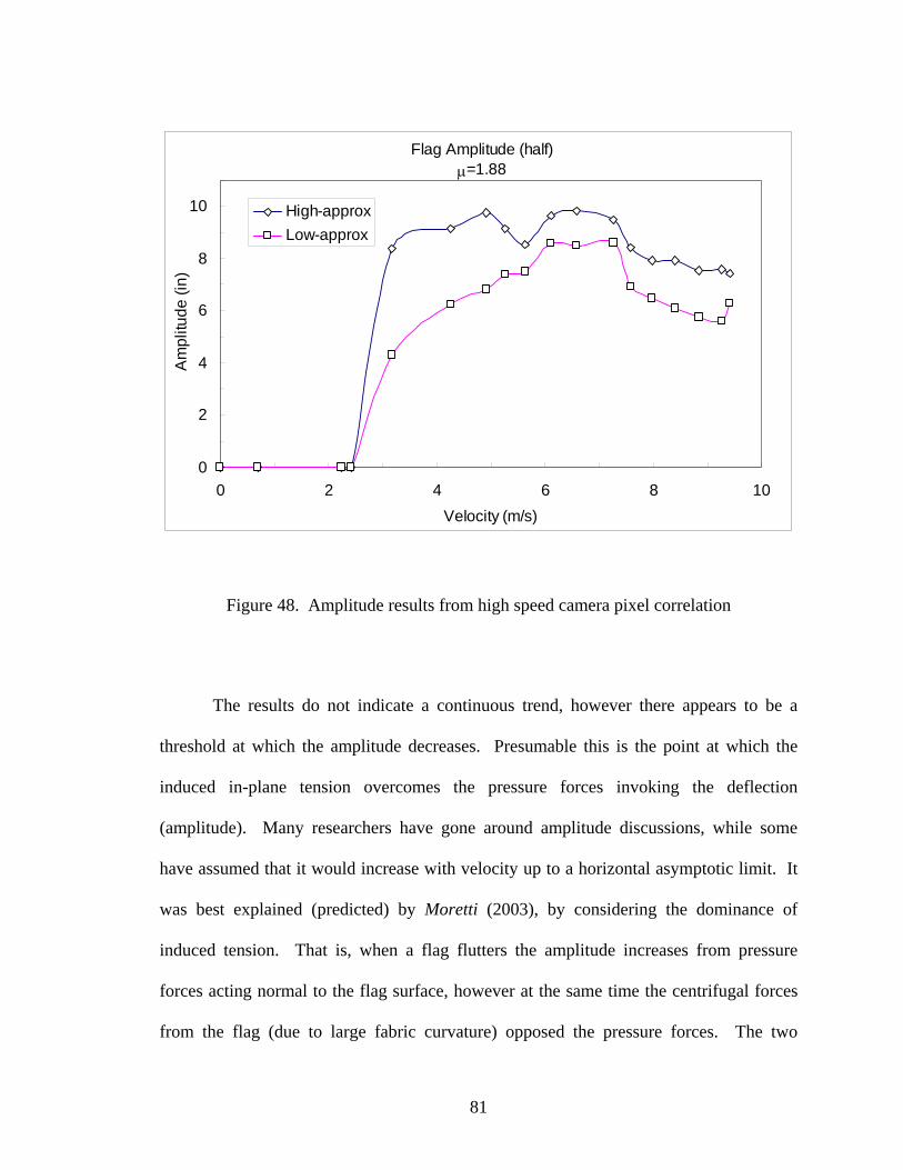
81
Flag Amplitude (half)μ=1.88
0
2
4
6
8
10
0 2 4 6 8 10Velocity (m/s)
Am
plitu
de (i
n)
High-approxLow-approx
Figure 48. Amplitude results from high speed camera pixel correlation
The results do not indicate a continuous trend, however there appears to be a
threshold at which the amplitude decreases. Presumable this is the point at which the
induced in-plane tension overcomes the pressure forces invoking the deflection
(amplitude). Many researchers have gone around amplitude discussions, while some
have assumed that it would increase with velocity up to a horizontal asymptotic limit. It
was best explained (predicted) by Moretti (2003), by considering the dominance of
induced tension. That is, when a flag flutters the amplitude increases from pressure
forces acting normal to the flag surface, however at the same time the centrifugal forces
from the flag (due to large fabric curvature) opposed the pressure forces. The two

82
phenomena are fighting each other. The pressure forces impose curvature and promote
large deflections, meanwhile the induced tension (in-plane with the fabric) work to
“straighten” the flag. At higher wind velocities, the amplitude results show that the
induced tension wins, and dominate the total drag at the attachment pole, thereby
reducing the amplitude. Analytical drag predictions suggested by Thoma (1939 b) and
Moretti (2003) are compared with experimental load cell data in Figure 49 and illustrate a
remarkable correlation, especially considering the first four data points have no flutter
frequency ( )0A ω= = . These first four data points represent the initial phase of the
experiment where the flag is being raised horizontally (parallel to the flow field).
Flag Drag Force Mass Ratio μ=1.88
0
0.25
0.5
0.75
1
1.25
0 2 4 6 8 10Velocity (m/s)
Dra
g (lb
f)
Exp. DragThoma/Moretti
2 214 flagT m A ω=
Figure 49. Experimental comparison of drag with theory [Thoma / Moretti]
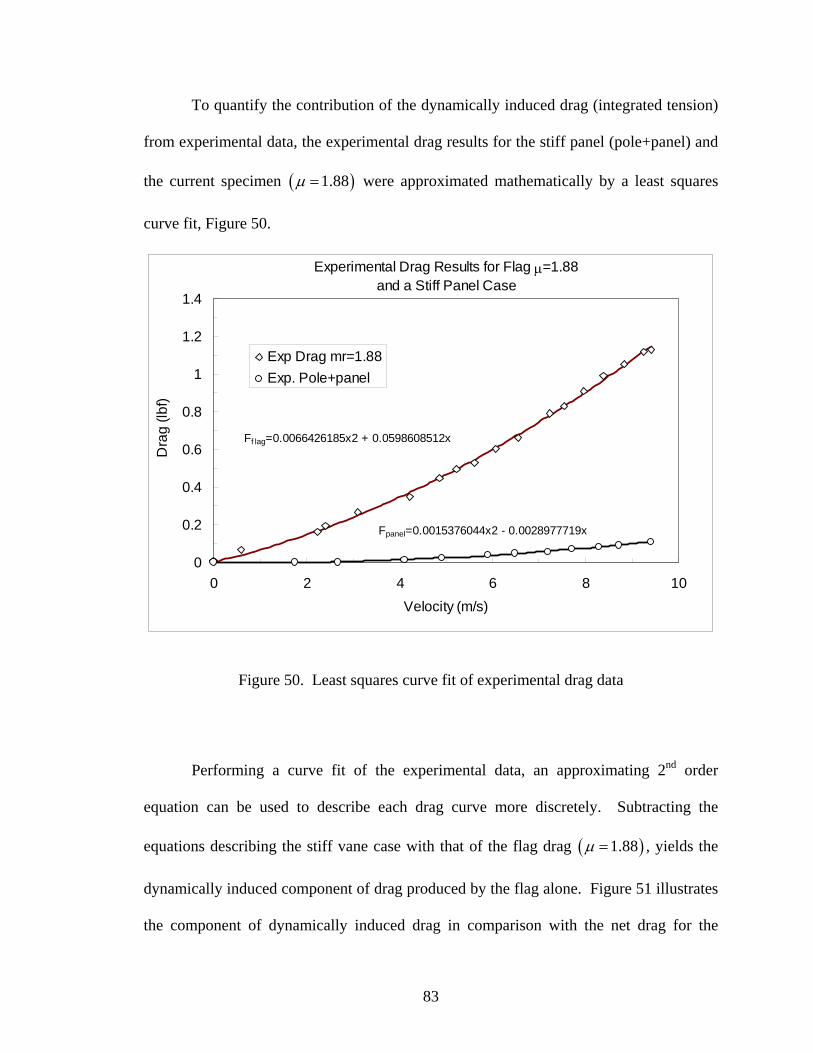
83
To quantify the contribution of the dynamically induced drag (integrated tension)
from experimental data, the experimental drag results for the stiff panel (pole+panel) and
the current specimen ( )1.88μ = were approximated mathematically by a least squares
curve fit, Figure 50.
Experimental Drag Results for Flag μ=1.88 and a Stiff Panel Case
0
0.2
0.4
0.6
0.8
1
1.2
1.4
0 2 4 6 8 10Velocity (m/s)
Dra
g (lb
f)
Exp Drag mr=1.88Exp. Pole+panel
Fpanel=0.0015376044x2 - 0.0028977719x
Ff lag=0.0066426185x2 + 0.0598608512x
Figure 50. Least squares curve fit of experimental drag data
Performing a curve fit of the experimental data, an approximating 2nd order
equation can be used to describe each drag curve more discretely. Subtracting the
equations describing the stiff vane case with that of the flag drag ( )1.88μ = , yields the
dynamically induced component of drag produced by the flag alone. Figure 51 illustrates
the component of dynamically induced drag in comparison with the net drag for the
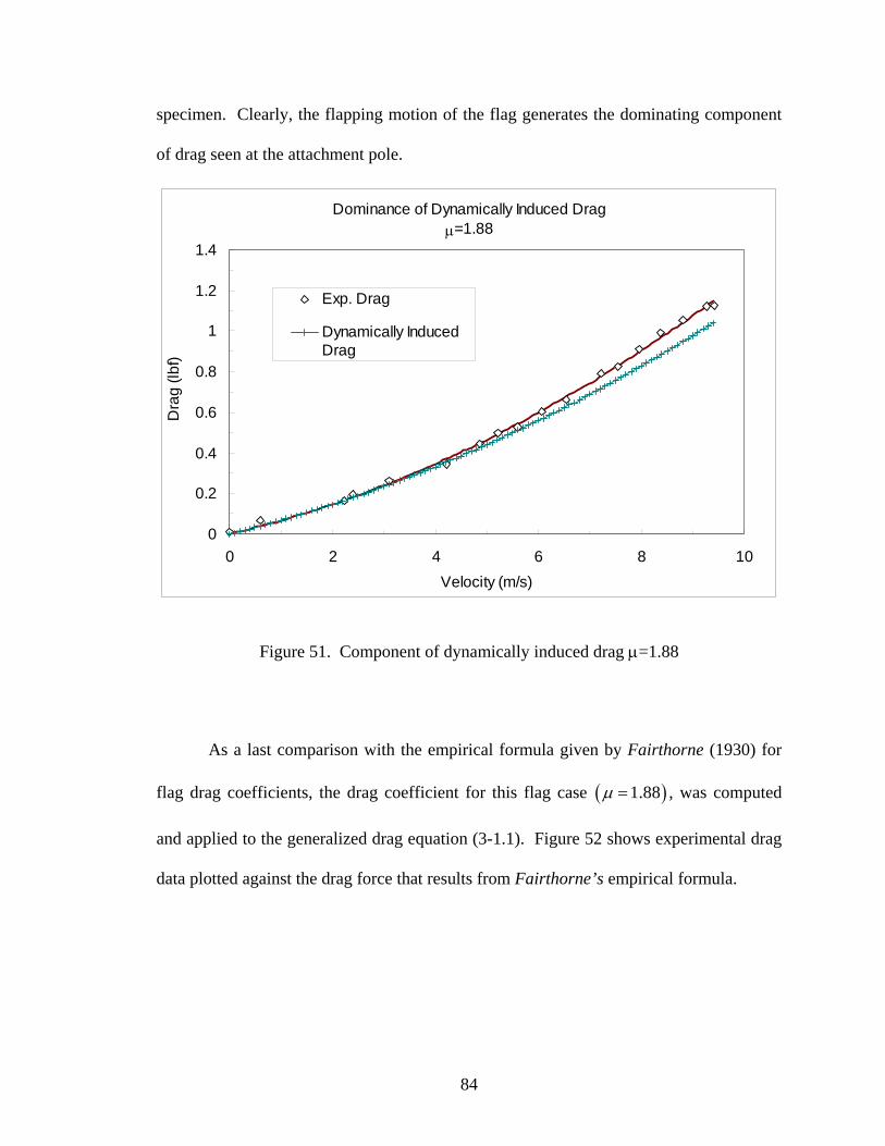
84
specimen. Clearly, the flapping motion of the flag generates the dominating component
of drag seen at the attachment pole.
Dominance of Dynamically Induced Dragμ=1.88
0
0.2
0.4
0.6
0.8
1
1.2
1.4
0 2 4 6 8 10Velocity (m/s)
Dra
g (lb
f)
Exp. Drag
Dynamically InducedDrag
Figure 51. Component of dynamically induced drag μ=1.88
As a last comparison with the empirical formula given by Fairthorne (1930) for
flag drag coefficients, the drag coefficient for this flag case ( )1.88μ = , was computed
and applied to the generalized drag equation (3-1.1). Figure 52 shows experimental drag
data plotted against the drag force that results from Fairthorne’s empirical formula.
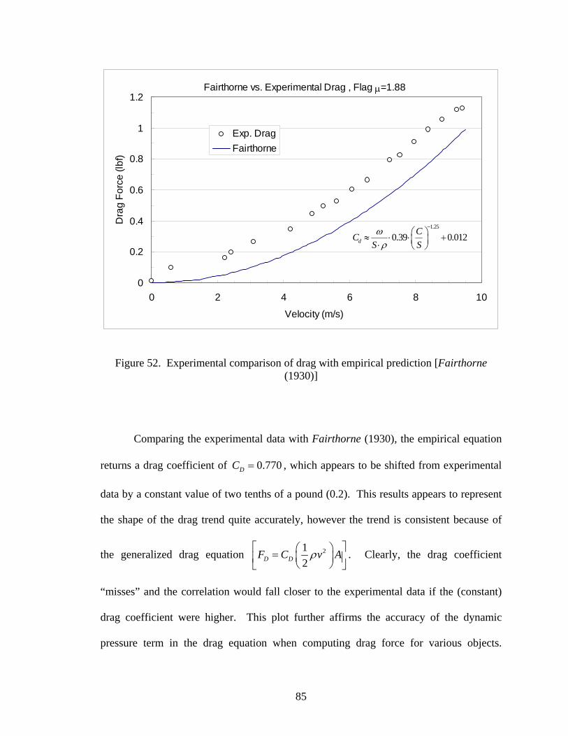
85
Fairthorne vs. Experimental Drag , Flag μ=1.88
0
0.2
0.4
0.6
0.8
1
1.2
0 2 4 6 8 10
Velocity (m/s)
Dra
g Fo
rce
(lbf)
Exp. DragFairthorne
1.25
0.39 0.012dCC
S Sω
ρ
−⎛ ⎞≈ ⋅ ⋅ +⎜ ⎟⋅ ⎝ ⎠
Figure 52. Experimental comparison of drag with empirical prediction [Fairthorne (1930)]
Comparing the experimental data with Fairthorne (1930), the empirical equation
returns a drag coefficient of 0.770DC = , which appears to be shifted from experimental
data by a constant value of two tenths of a pound (0.2). This results appears to represent
the shape of the drag trend quite accurately, however the trend is consistent because of
the generalized drag equation 212D DF C v Aρ⎡ ⎤⎛ ⎞= ⎜ ⎟⎢ ⎥⎝ ⎠⎣ ⎦
. Clearly, the drag coefficient
“misses” and the correlation would fall closer to the experimental data if the (constant)
drag coefficient were higher. This plot further affirms the accuracy of the dynamic
pressure term in the drag equation when computing drag force for various objects.
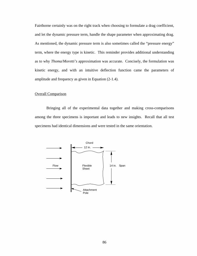
86
Fairthorne certainly was on the right track when choosing to formulate a drag coefficient,
and let the dynamic pressure term, handle the shape parameter when approximating drag.
As mentioned, the dynamic pressure term is also sometimes called the “pressure energy”
term, where the energy type is kinetic. This reminder provides additional understanding
as to why Thoma/Moretti’s approximation was accurate. Concisely, the formulation was
kinetic energy, and with an intuitive deflection function came the parameters of
amplitude and frequency as given in Equation (2-1.4).
Overall Comparison
Bringing all of the experimental data together and making cross-comparisons
among the three specimens is important and leads to new insights. Recall that all test
specimens had identical dimensions and were tested in the same orientation.
FlexibleSheet
Chord
Span
AttachmentPole
14 in.
12 in.
Flow
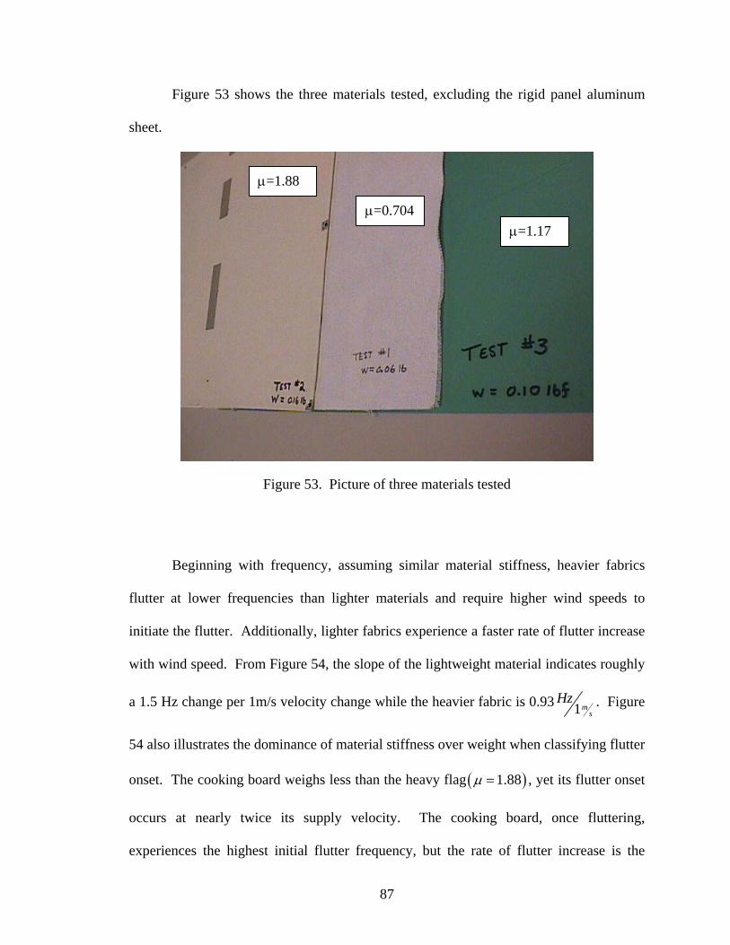
87
Figure 53 shows the three materials tested, excluding the rigid panel aluminum
sheet.
Figure 53. Picture of three materials tested
Beginning with frequency, assuming similar material stiffness, heavier fabrics
flutter at lower frequencies than lighter materials and require higher wind speeds to
initiate the flutter. Additionally, lighter fabrics experience a faster rate of flutter increase
with wind speed. From Figure 54, the slope of the lightweight material indicates roughly
a 1.5 Hz change per 1m/s velocity change while the heavier fabric is 0.93 1ms
Hz . Figure
54 also illustrates the dominance of material stiffness over weight when classifying flutter
onset. The cooking board weighs less than the heavy flag ( )1.88μ = , yet its flutter onset
occurs at nearly twice its supply velocity. The cooking board, once fluttering,
experiences the highest initial flutter frequency, but the rate of flutter increase is the
μ=1.17 μ=0.704
μ=1.88
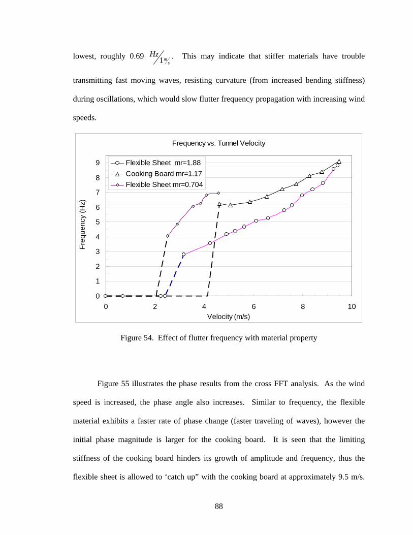
88
lowest, roughly 0.69 1ms
Hz . This may indicate that stiffer materials have trouble
transmitting fast moving waves, resisting curvature (from increased bending stiffness)
during oscillations, which would slow flutter frequency propagation with increasing wind
speeds.
Frequency vs. Tunnel Velocity
0
1
2
3
4
5
6
7
8
9
0 2 4 6 8 10Velocity (m/s)
Freq
uenc
y (H
z)
Flexible Sheet mr=1.88Cooking Board mr=1.17Flexible Sheet mr=0.704
Figure 54. Effect of flutter frequency with material property
Figure 55 illustrates the phase results from the cross FFT analysis. As the wind
speed is increased, the phase angle also increases. Similar to frequency, the flexible
material exhibits a faster rate of phase change (faster traveling of waves), however the
initial phase magnitude is larger for the cooking board. It is seen that the limiting
stiffness of the cooking board hinders its growth of amplitude and frequency, thus the
flexible sheet is allowed to ‘catch up” with the cooking board at approximately 9.5 m/s.
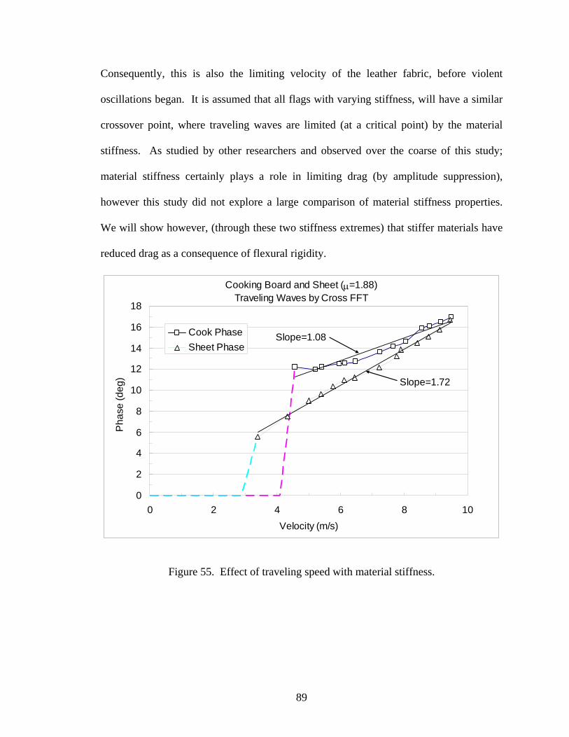
89
Consequently, this is also the limiting velocity of the leather fabric, before violent
oscillations began. It is assumed that all flags with varying stiffness, will have a similar
crossover point, where traveling waves are limited (at a critical point) by the material
stiffness. As studied by other researchers and observed over the coarse of this study;
material stiffness certainly plays a role in limiting drag (by amplitude suppression),
however this study did not explore a large comparison of material stiffness properties.
We will show however, (through these two stiffness extremes) that stiffer materials have
reduced drag as a consequence of flexural rigidity.
Cooking Board and Sheet (μ=1.88)Traveling Waves by Cross FFT
0
2
4
6
8
10
12
14
16
18
0 2 4 6 8 10Velocity (m/s)
Pha
se (d
eg)
Cook PhaseSheet Phase
Slope=1.72
Slope=1.08
Figure 55. Effect of traveling speed with material stiffness.
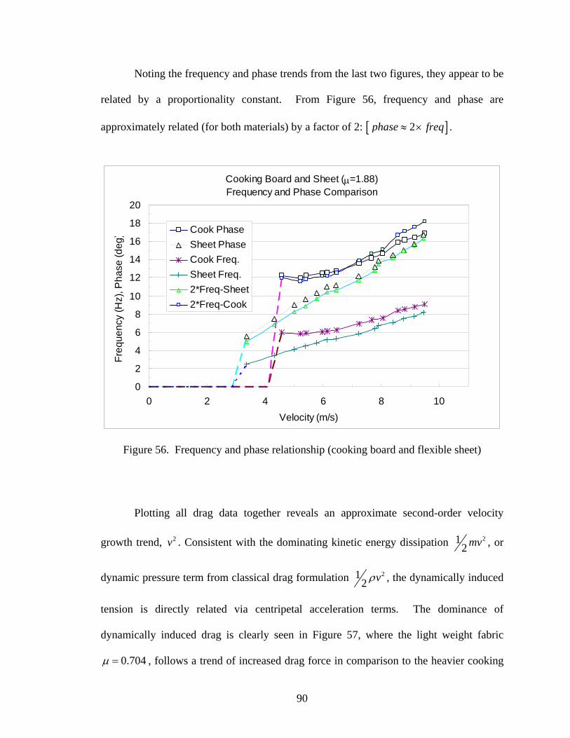
90
Noting the frequency and phase trends from the last two figures, they appear to be
related by a proportionality constant. From Figure 56, frequency and phase are
approximately related (for both materials) by a factor of 2: [ ]2phase freq≈ × .
Cooking Board and Sheet (μ=1.88)Frequency and Phase Comparison
0
2
4
6
8
10
12
14
16
18
20
0 2 4 6 8 10Velocity (m/s)
Freq
uenc
y (H
z), P
hase
(deg
) Cook PhaseSheet PhaseCook Freq.Sheet Freq.2*Freq-Sheet2*Freq-Cook
Figure 56. Frequency and phase relationship (cooking board and flexible sheet)
Plotting all drag data together reveals an approximate second-order velocity
growth trend, 2v . Consistent with the dominating kinetic energy dissipation 212 mv , or
dynamic pressure term from classical drag formulation 212 vρ , the dynamically induced
tension is directly related via centripetal acceleration terms. The dominance of
dynamically induced drag is clearly seen in Figure 57, where the light weight fabric
0.704μ = , follows a trend of increased drag force in comparison to the heavier cooking
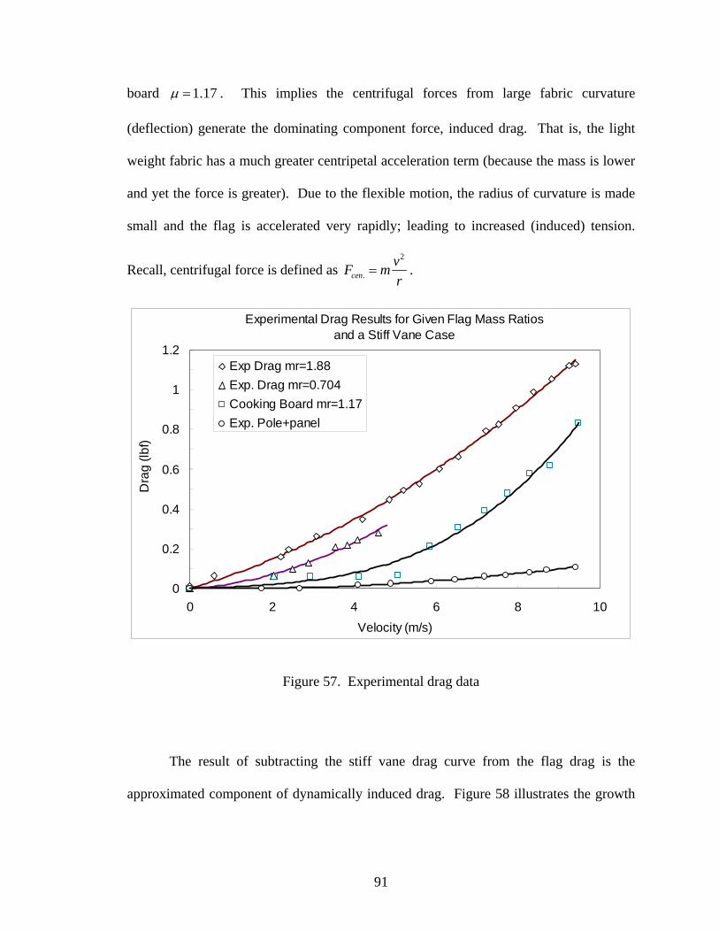
91
board 1.17μ = . This implies the centrifugal forces from large fabric curvature
(deflection) generate the dominating component force, induced drag. That is, the light
weight fabric has a much greater centripetal acceleration term (because the mass is lower
and yet the force is greater). Due to the flexible motion, the radius of curvature is made
small and the flag is accelerated very rapidly; leading to increased (induced) tension.
Recall, centrifugal force is defined as 2
.cenvF mr
= .
Experimental Drag Results for Given Flag Mass Ratios and a Stiff Vane Case
0
0.2
0.4
0.6
0.8
1
1.2
0 2 4 6 8 10Velocity (m/s)
Dra
g (lb
f)
Exp Drag mr=1.88Exp. Drag mr=0.704Cooking Board mr=1.17Exp. Pole+panel
Figure 57. Experimental drag data
The result of subtracting the stiff vane drag curve from the flag drag is the
approximated component of dynamically induced drag. Figure 58 illustrates the growth
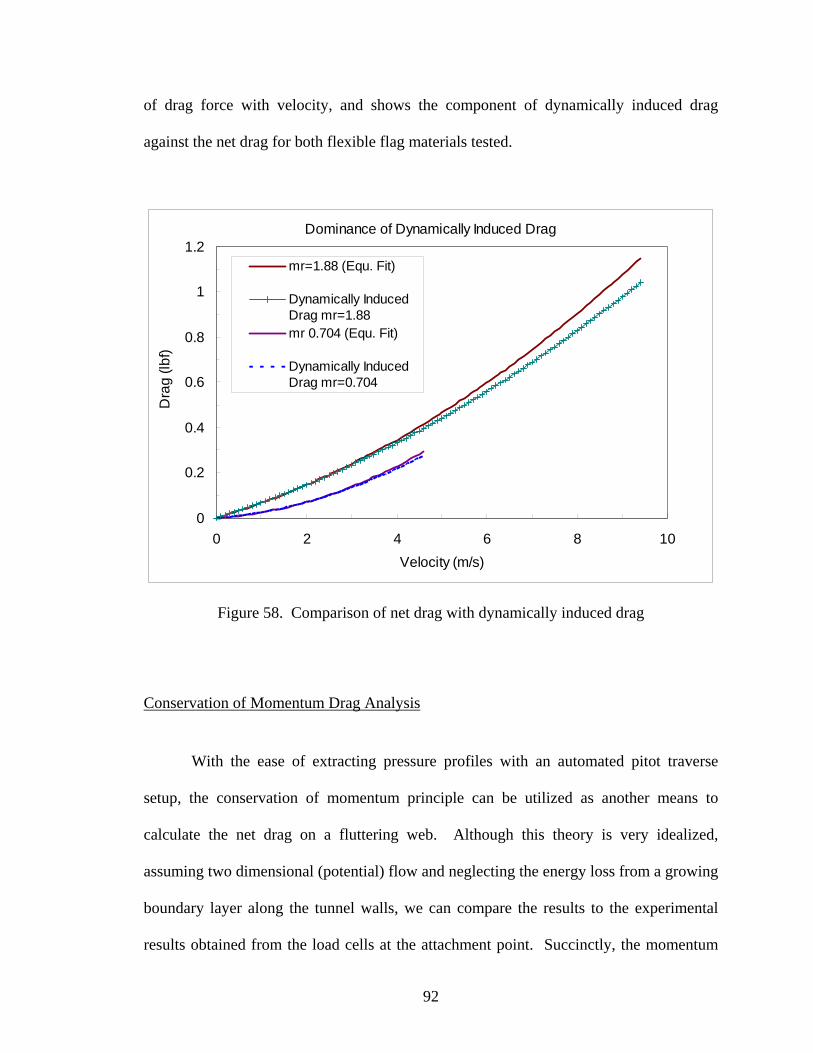
92
of drag force with velocity, and shows the component of dynamically induced drag
against the net drag for both flexible flag materials tested.
Dominance of Dynamically Induced Drag
0
0.2
0.4
0.6
0.8
1
1.2
0 2 4 6 8 10Velocity (m/s)
Dra
g (lb
f)
mr=1.88 (Equ. Fit)
Dynamically InducedDrag mr=1.88mr 0.704 (Equ. Fit)
Dynamically InducedDrag mr=0.704
Figure 58. Comparison of net drag with dynamically induced drag
Conservation of Momentum Drag Analysis
With the ease of extracting pressure profiles with an automated pitot traverse
setup, the conservation of momentum principle can be utilized as another means to
calculate the net drag on a fluttering web. Although this theory is very idealized,
assuming two dimensional (potential) flow and neglecting the energy loss from a growing
boundary layer along the tunnel walls, we can compare the results to the experimental
results obtained from the load cells at the attachment point. Succinctly, the momentum
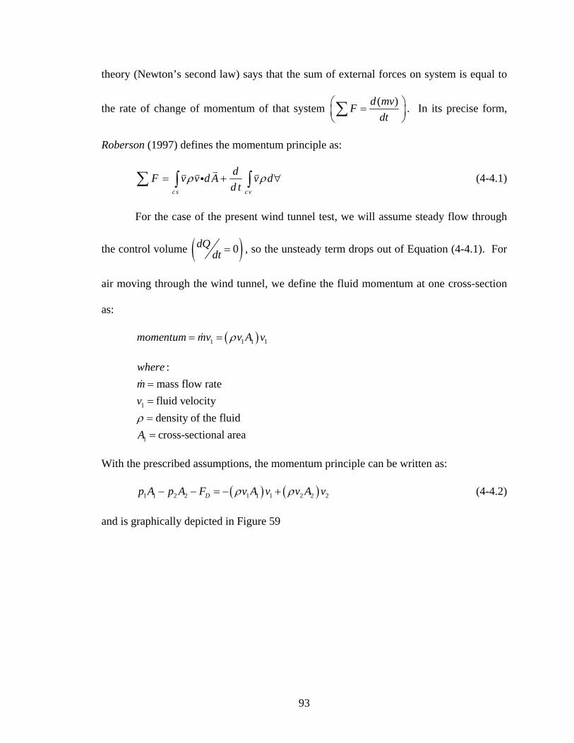
93
theory (Newton’s second law) says that the sum of external forces on system is equal to
the rate of change of momentum of that system ( )d mvFdt
⎛ ⎞=⎜ ⎟⎝ ⎠∑ . In its precise form,
Roberson (1997) defines the momentum principle as:
c s c v
dF v v d A v dd t
ρ ρ= + ∀∑ ∫ ∫i (4-4.1)
For the case of the present wind tunnel test, we will assume steady flow through
the control volume ( )0dQdt = , so the unsteady term drops out of Equation (4-4.1). For
air moving through the wind tunnel, we define the fluid momentum at one cross-section
as:
( )1 1 1 1momentum mv v A vρ= =
1
1
:mass flow ratefluid velocity density of the fluidcross-sectional area
wheremv
Aρ
====
With the prescribed assumptions, the momentum principle can be written as:
( ) ( )1 1 2 2 1 1 1 2 2 2Dp A p A F v A v v A vρ ρ− − = − + (4-4.2)
and is graphically depicted in Figure 59
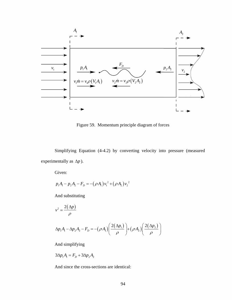
94
Figure 59. Momentum principle diagram of forces
Simplifying Equation (4-4.2) by converting velocity into pressure (measured
experimentally as pΔ ).
Given:
( ) ( )2 21 1 2 2 1 1 2 2Dp A p A F A v A vρ ρ− − = − +
And substituting
( )2 2 pv
ρΔ
=
( ) ( ) ( ) ( )1 21 1 2 2 1 2
2 2D
p pp A p A F A Aρ ρ
ρ ρΔ Δ⎛ ⎞ ⎛ ⎞
Δ − Δ − = − +⎜ ⎟ ⎜ ⎟⎝ ⎠ ⎝ ⎠
And simplifying
1 1 2 23 3Dp A F p AΔ = + Δ
And since the cross-sections are identical:
( )1 1 1 1v m v V Aρ= ( )2 2 2 2v m v V Aρ=
2v1v 1 1p A 2 2p ADF
2A1A
95
( )1 23DF A p p= Δ − Δ (4-4.3)
Equation (4-4.3) describes the theoretical drag force for the object disrupting the
flow (attachment pole and sheet) assuming the pressure distribution is constant at the
upstream and downstream cross-sections. Experimentally, a 26 26 .in× inch area
centered on the wind tunnel’s 36 36 .in× cross-section is traversed in 1 .in increments.
Pressure readings from the pitot tube thus discretize the flow field into 21 in areas ( )A∗ .
The conservation of momentum is directly applied as:
, ,
26 26
1 21 1
3i j i j
Dj i
F A p p∗ ∗ ∗ ∗
∗
= =
⎛ ⎞= Δ − Δ⎜ ⎟⎝ ⎠∑∑
1 ,1 2 ,1 3 ,1 26 ,11 ,1 2 ,1 3 ,1 26 ,1
1 ,2 2 ,2 3 ,2 26 ,21 ,2 2 ,2 3 ,2 26 ,2
1 2 1 2 1 2 1 2
1 2 1 2 1 2 1 23D
or
p p p p p p p p
F A p p p p p p p p
∗ ∗ ∗ ∗ ∗ ∗ ∗ ∗∗ ∗ ∗ ∗ ∗ ∗ ∗ ∗
∗ ∗ ∗ ∗ ∗ ∗ ∗ ∗∗ ∗ ∗ ∗ ∗ ∗ ∗ ∗
∗
⎛ ⎞ ⎛ ⎞ ⎛ ⎞ ⎛ ⎞Δ − Δ + Δ − Δ + Δ − Δ + Δ − Δ⎜ ⎟ ⎜ ⎟ ⎜ ⎟ ⎜ ⎟⎝ ⎠ ⎝ ⎠ ⎝ ⎠ ⎝ ⎠
⎛ ⎞ ⎛ ⎞ ⎛ ⎞ ⎛= + Δ − Δ + Δ − Δ + Δ − Δ + Δ − Δ⎜ ⎟ ⎜ ⎟ ⎜ ⎟⎝ ⎠ ⎝ ⎠ ⎝ ⎠
…
…
26 ,26 26 ,261 2 p p
∗ ∗ ∗ ∗
⎡ ⎤⎢ ⎥⎢ ⎥
⎞⎢ ⎥⎜ ⎟⎢ ⎥⎝ ⎠⎢ ⎥
⎛ ⎞⎢ ⎥+ Δ − Δ⎜ ⎟⎢ ⎥⎝ ⎠⎣ ⎦…
The 5 inch gap between the wind tunnel wall and the outer perimeter of the swept
area will not be accounted for, but assumed to have an equal pressure distribution.
Experiments reveal that the boundary layer thickness is roughly 2 inches (Chambers
1999). From boundary layer theory and experimental data, the boundary layer will grow
as fluid progresses down the length of the tunnel. The increase in boundary layer
thickness downstream of the tunnel section will produce larger viscous forces, and hence
fluid momentum loss. This loss will create a slight pressure drop from the wind tunnel
entrance to the exit. This phenomenon was confirmed by utilizing pressure taps aligned
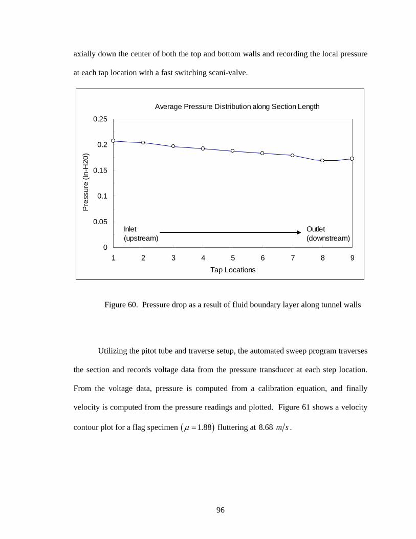
96
axially down the center of both the top and bottom walls and recording the local pressure
at each tap location with a fast switching scani-valve.
Average Pressure Distribution along Section Length
0
0.05
0.1
0.15
0.2
0.25
1 2 3 4 5 6 7 8 9Tap Locations
Pre
ssur
e (In
-H20
)
Inlet(upstream)
Outlet(downstream)
Figure 60. Pressure drop as a result of fluid boundary layer along tunnel walls
Utilizing the pitot tube and traverse setup, the automated sweep program traverses
the section and records voltage data from the pressure transducer at each step location.
From the voltage data, pressure is computed from a calibration equation, and finally
velocity is computed from the pressure readings and plotted. Figure 61 shows a velocity
contour plot for a flag specimen ( )1.88μ = fluttering at 8.68 m s .
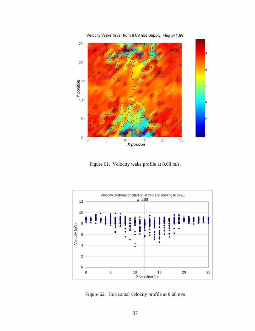
97
Figure 61. Velocity wake profile at 8.68 m/s.
Velocity Distribution starting at x=0 and moving to x=25μ=1.88
0
2
4
6
8
10
12
0 5 10 15 20 25X direction (in)
Vel
ocity
(m/s
)
Figure 62. Horizontal velocity profile at 8.68 m/s
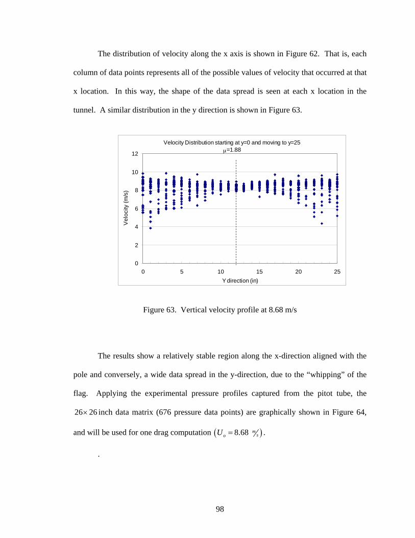
98
The distribution of velocity along the x axis is shown in Figure 62. That is, each
column of data points represents all of the possible values of velocity that occurred at that
x location. In this way, the shape of the data spread is seen at each x location in the
tunnel. A similar distribution in the y direction is shown in Figure 63.
Velocity Distribution starting at y=0 and moving to y=25
μ=1.88
0
2
4
6
8
10
12
0 5 10 15 20 25Y direction (in)
Vel
ocity
(m/s
)
Figure 63. Vertical velocity profile at 8.68 m/s
The results show a relatively stable region along the x-direction aligned with the
pole and conversely, a wide data spread in the y-direction, due to the “whipping” of the
flag. Applying the experimental pressure profiles captured from the pitot tube, the
26 26× inch data matrix (676 pressure data points) are graphically shown in Figure 64,
and will be used for one drag computation ( )8.68 msoU = .
.
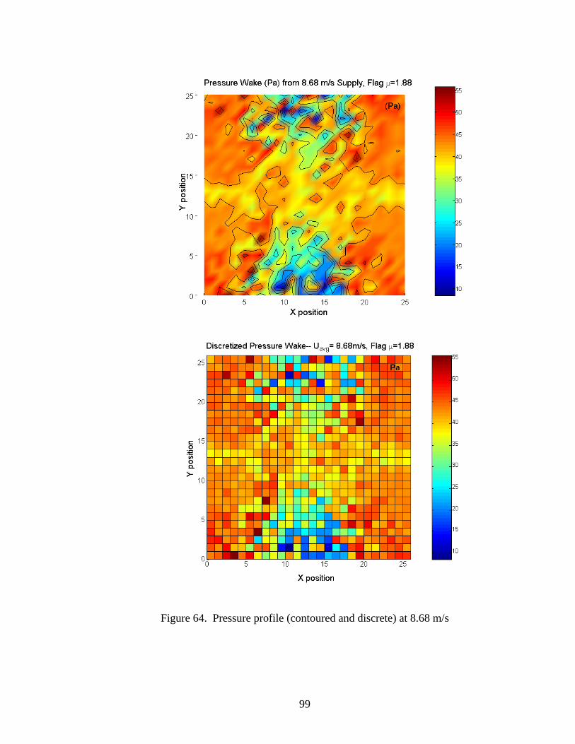
99
Figure 64. Pressure profile (contoured and discrete) at 8.68 m/s
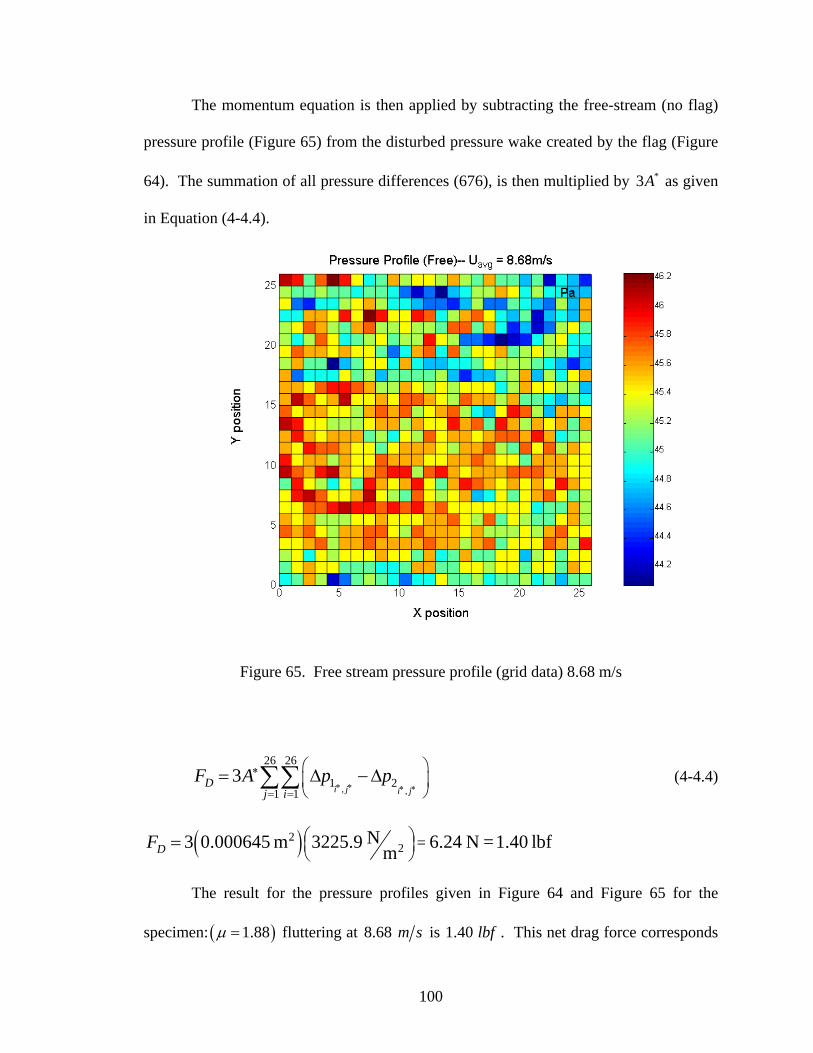
100
The momentum equation is then applied by subtracting the free-stream (no flag)
pressure profile (Figure 65) from the disturbed pressure wake created by the flag (Figure
64). The summation of all pressure differences (676), is then multiplied by *3A as given
in Equation (4-4.4).
Figure 65. Free stream pressure profile (grid data) 8.68 m/s
, ,
26 26
1 21 1
3i j i j
Dj i
F A p p∗ ∗ ∗ ∗
∗
= =
⎛ ⎞⎜ ⎟⎝ ⎠
= Δ − Δ∑∑ (4-4.4)
( )22 =N3 0.000645 m 3225.9 6.24 N =1.40 lbfmDF ⎛ ⎞⎜ ⎟
⎝ ⎠=
The result for the pressure profiles given in Figure 64 and Figure 65 for the
specimen: ( )1.88μ = fluttering at 8.68 m s is 1.40 lbf . This net drag force corresponds
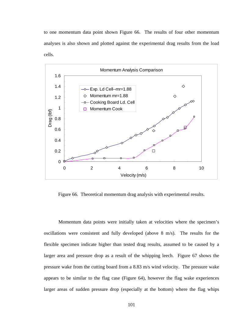
101
to one momentum data point shown Figure 66. The results of four other momentum
analyses is also shown and plotted against the experimental drag results from the load
cells.
Momentum Analysis Comparison
0
0.2
0.4
0.6
0.8
1
1.2
1.4
1.6
0 2 4 6 8 10Velocity (m/s)
Dra
g (lb
f)
Exp. Ld Cell--mr=1.88Momentum mr=1.88Cooking Board Ld. CellMomentum Cook
Figure 66. Theoretical momentum drag analysis with experimental results.
Momentum data points were initially taken at velocities where the specimen’s
oscillations were consistent and fully developed (above 8 m/s). The results for the
flexible specimen indicate higher than tested drag results, assumed to be caused by a
larger area and pressure drop as a result of the whipping leech. Figure 67 shows the
pressure wake from the cutting board from a 8.83 m/s wind velocity. The pressure wake
appears to be similar to the flag case (Figure 64), however the flag wake experiences
larger areas of sudden pressure drop (especially at the bottom) where the flag whips
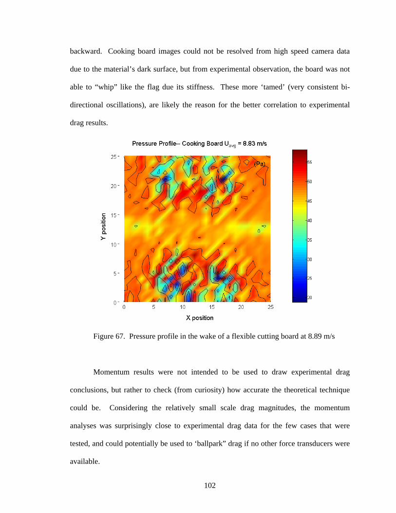
102
backward. Cooking board images could not be resolved from high speed camera data
due to the material’s dark surface, but from experimental observation, the board was not
able to “whip” like the flag due its stiffness. These more ‘tamed’ (very consistent bi-
directional oscillations), are likely the reason for the better correlation to experimental
drag results.
Figure 67. Pressure profile in the wake of a flexible cutting board at 8.89 m/s
Momentum results were not intended to be used to draw experimental drag
conclusions, but rather to check (from curiosity) how accurate the theoretical technique
could be. Considering the relatively small scale drag magnitudes, the momentum
analyses was surprisingly close to experimental drag data for the few cases that were
tested, and could potentially be used to ‘ballpark” drag if no other force transducers were
available.
103
CHAPTER V
CONCLUSIONS
Drag Overview
When a flag flutters, tension is induced (in-plane) from centrifugal forces due to
the flutter motion (out-of-plane). The induced tension acts to “flatten” the flag, however,
the pressure forces acting across (normal) to the flag, which generated the lift and
induced tension, are fighting to invoke curvature. The flow field generates lift forces on
the fabric that induce the in-plane tension, and because the flutter oscillations are
symmetrical about the attachment point and normal to the flow field, the time average lift
is felt only as the specimen’s weight (Figure 46)
We have learned that increased material stiffness leads to decreased drag. Recall
the stiff cutting board yielded smaller drag forces when compared with both flexible
sheets. Low stiffness in this test setting was even proven to override the inclusion of
added mass, as the light weight flexible specimen ( )0.704, 0.027 m kgμ = = weighed
less than the cutting board ( )1.74, 0.045 m kgμ = = and yet exhibited increased drag
force at the attachment. The large curvature from the fabrics (as a consequence of low
material stiffness) yielded large dynamically induced forces. The fact that we see lower
drag predictions by using Fairthorne’s drag coefficient approximation equation suggests
that there is a degree of structural stiffening that occurs with a change in flag dimensions.
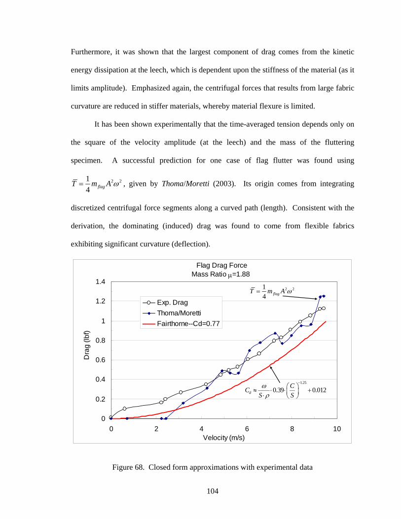
104
Furthermore, it was shown that the largest component of drag comes from the kinetic
energy dissipation at the leech, which is dependent upon the stiffness of the material (as it
limits amplitude). Emphasized again, the centrifugal forces that results from large fabric
curvature are reduced in stiffer materials, whereby material flexure is limited.
It has been shown experimentally that the time-averaged tension depends only on
the square of the velocity amplitude (at the leech) and the mass of the fluttering
specimen. A successful prediction for one case of flag flutter was found using
2 214 flagT m A ω= , given by Thoma/Moretti (2003). Its origin comes from integrating
discretized centrifugal force segments along a curved path (length). Consistent with the
derivation, the dominating (induced) drag was found to come from flexible fabrics
exhibiting significant curvature (deflection).
Flag Drag Force Mass Ratio μ=1.88
0
0.2
0.4
0.6
0.8
1
1.2
1.4
0 2 4 6 8 10Velocity (m/s)
Dra
g (lb
f)
Exp. DragThoma/MorettiFairthorne--Cd=0.77
1.25
0.39 0.012dCC
S Sω
ρ
−⎛ ⎞≈ ⋅ ⋅ +⎜ ⎟⋅ ⎝ ⎠
2 214 flagT m A ω=
Figure 68. Closed form approximations with experimental data
105
Wave Characteristics
Vibrometer phase computations and high speed camera images confirm both the
presence of a traveling and standing waves. Superimposed images reveal partial
traveling nodes and suggest a small stationary anti-node. The combination of such, are
indicative of traveling and standing waves, with a wave ratio greater than unity, and an
overwhelming dominance of traveling waves. Furthermore, it was shown that stiffer
materials flutter at higher frequencies and have larger phase angles, indicating they are
able to transmit the fluid energy more efficiently. Stiffer materials have faster traveling
waves up to a critical velocity point, thereafter flexible sheets will travel faster. This
attribute can again be related back to the stiffness property limiting the natural
progression (growth) of the waveform. Interestingly, both the flexible and stiff material
tested exhibited a phase angle of approximately twice the fundamental fluttering
frequency.
Perhaps a new discovery has come from the ability to measure the amplitude at
the leech with a high speed camera. Figure 69 illustrates a sudden increase in amplitude
upon flutter onset, followed by a bell shape curve, where the amplitude peaks and tapers
off. At this point, it is believed in-plane induced tension from centrifugal forces are
competing with the normal pressure forces that create the amplitude deflection. At higher
wind velocities, the amplitude results show that the induced tension wins, and dominate
the total drag at the attachment pole, thereby reducing the amplitude
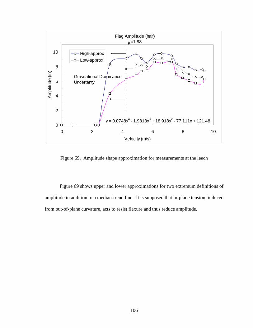
106
Flag Amplitude (half)μ=1.88
y = 0.0748x4 - 1.9813x3 + 18.918x2 - 77.111x + 121.480
2
4
6
8
10
0 2 4 6 8 10Velocity (m/s)
Am
plitu
de (i
n)High-approxLow-approx
Gravitational DominanceUncertanty
Figure 69. Amplitude shape approximation for measurements at the leech
Figure 69 shows upper and lower approximations for two extremum definitions of
amplitude in addition to a median-trend line. It is supposed that in-plane tension, induced
from out-of-plane curvature, acts to resist flexure and thus reduce amplitude.

107
REFERENCES
Bishop, R.H., 1999. Learning with LabVIEW. Addison Wesley Longman, Inc. Menlo
Park, California, pp. 394-404.
Chambers, F.W., 2005. Associate Professor in Mechanical and Aerospace Engineering,
Oklahoma State University. Private Communication.
Fairthorne, R.A., 1930. “Drag of Flags”, Aeronautical Research Committee (ARC)
Reports and Memoranda No. 1345 (Ae.477), Her Majesty’s Printing Office
(HMSO), London, pp. 887-891.
Hoerner, S.F., 1958. Fluid Dynamic Drag, Hoerner Fluid Dynamics, Brick Town, N.J.,
section 3, p 25.
Holman,.J.P., 1995. Experimental Methods for Engineers. New York: McGraw-Hill, pp.
59-62.
Moretti P. M., 2003. “Tension in Fluttering Flags”, International Journal of Acoustics
and Vibration, Vol. 4, No. 4, pp.227-230.
Mott, R. L, 2000. Applied Fluid Mechanics, 5th Edition, Prentice Hall, Upper Saddle, NJ,
pp. 485-495.

108
Roberson, J. A & Crowe, C. T., 1997. Engineering Fluid Mechanics, 6th Edition, John
Wiley and Sons, Inc., Toronto, pp. 429-453.
Taneda, S., 1968. “Waving Motions of Flags”, J. of the Physical Society of Japan, Vol
24, No.2, pp. 392-401.
Thoma, D., 1939 a. “Warum Flattert die Fahne”, Mitteilungen des Hydraulischen
Instituts der Technischen Hochschule Muechen, No. 9, pages 30-34; translation
“Why does the Flag Flutter”, Cornell Aeronautical Laboratory, (1949).
Thoma, D., 1939 b. “Das schlenkernde Seil”, Zeitschrift der Angewandten Mathematik
und Mechanik, (ZAAM) No. 19, pages 320-321; translation “The oscillating
Rope”.
Uno, M., 1973. “Fluttering of Flexible Bodies”, J. of the Textile Machinery Society of
Japan, Vol.19, No.4-5, pp.103-109.
Watanabe, Y., Suzuki, S., Sugihara, M., & Sueoka, Y., 2002. “An Experimental Study of
Paper Flutter”, J. of the Fluids and Structures, Vol.16, No.4, pp.529-542.
Yamaguchi, N., Sekiguchi, T., Yokota, K., Tsujimoto, Y., 2000. “Flutter Limits and
Behavior of a Flexible Thin Sheet in High–Speed Flow—II: Experimental Results
and Predicted Behaviors for Low Mass Ratios”, Trans. ASME, J. of Fluids
Engineering, Vol 122, pp. 74-83.

109
APPENDICES
APPENDIX A—WIND TUNNEL TEST SECTION DRAWINGS...............................110
APPENDIX B—MATLAB VELOCITY CONTOUR M-FILE......................................114
APPENDIX C—STEPPING MOTOR WIRING SCHEMATIC....................................115
APPENDIX D—STEPPING MOTOR DRIVER CIRCUIT...........................................117
APPENDIX E—LABVIEW PITOT TRAVERSE MOTOR CONTROL.......................118
APPENDIX F—PITOT TUBE PRESSURE UNCERTAINTY......................................119
APPENDIX G—MATLAB CROSS-POWER-SPECTRUM M-FILE ...........................121
APPENDIX H—LABVIEW FFT FRONT PANEL POWER SPECTRUM VI. ............125
APPENDIX I—EXCEL SHEET AIR PROPERTY CALCULATOR............................126
APPENDIX J—EXCEL AIR PROPERTY CALCULATOR FORMULAS ..................127
APPENDIX K—FREE-STREAM PRESSURE PROFILES ..........................................129
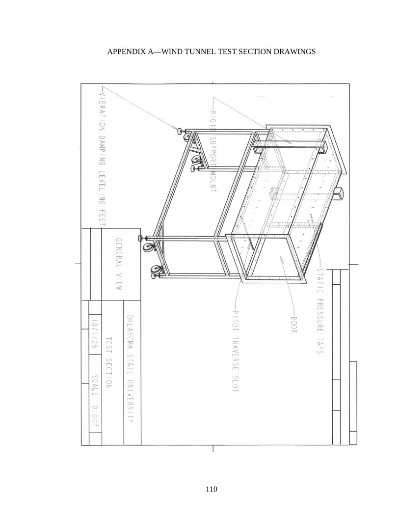
110
APPENDIX A—WIND TUNNEL TEST SECTION DRAWINGS
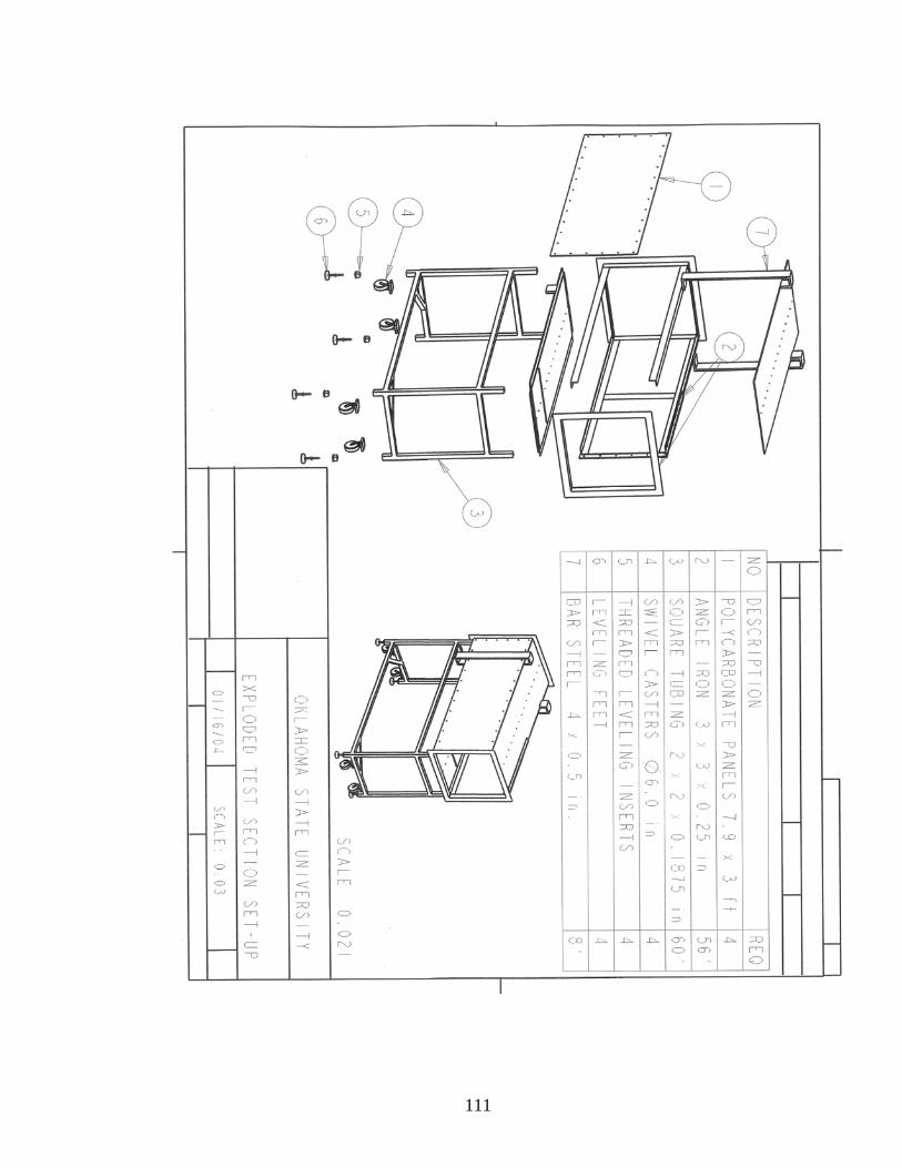
111
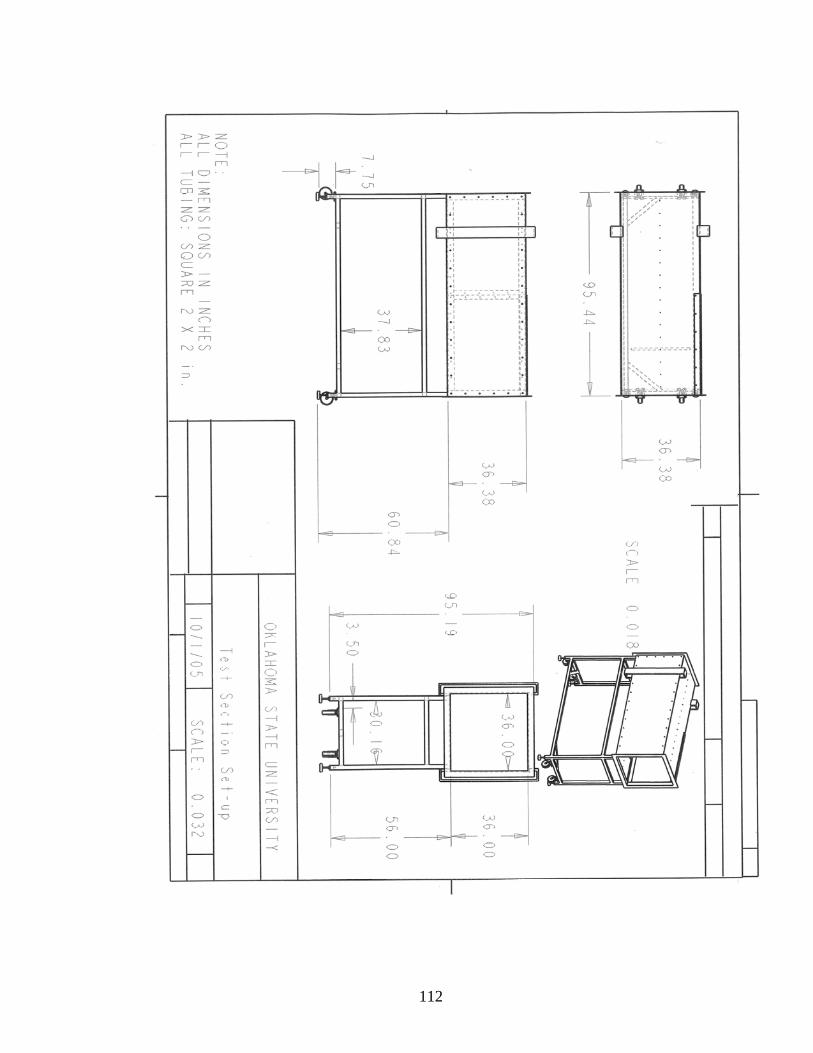
112
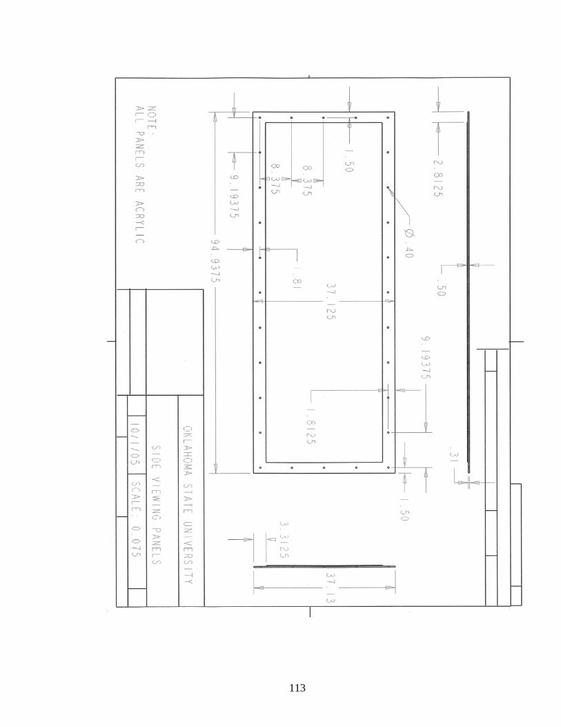
113

114
APPENDIX B—MATLAB VELOCITY CONTOUR M-FILE
%Pressure Contour M-file clear all; close all; clc; fprintf ( 1, '\n' ); fprintf ( 1, 'VELOCITY CONTOUR \n' ); fprintf ( 1, '\n' ); file = input('Enter Excel File Name: ','s'); fprintf ( 1, '\n' ); squaresweepsize = input('Enter Square Sweep Size: '); A=xlsread(file); x=(A(1:squaresweepsize^2,1)); y=(A(1:squaresweepsize^2,2)); z=(A(1:squaresweepsize^2,3)); XI=0:1:(squaresweepsize); YI=0:1:(squaresweepsize); ZI=griddata(x,y,z,XI,YI'); hold on pcolor(XI,YI,ZI); shading interp; axis equal; xlabel('X position'); ylabel('Y position'); title('Velocity Distribution'); colorbar; min1=min(z); max1=max(z); conts=min1:.1:max1; contour(XI,YI,ZI,conts,'k'); axis equal;
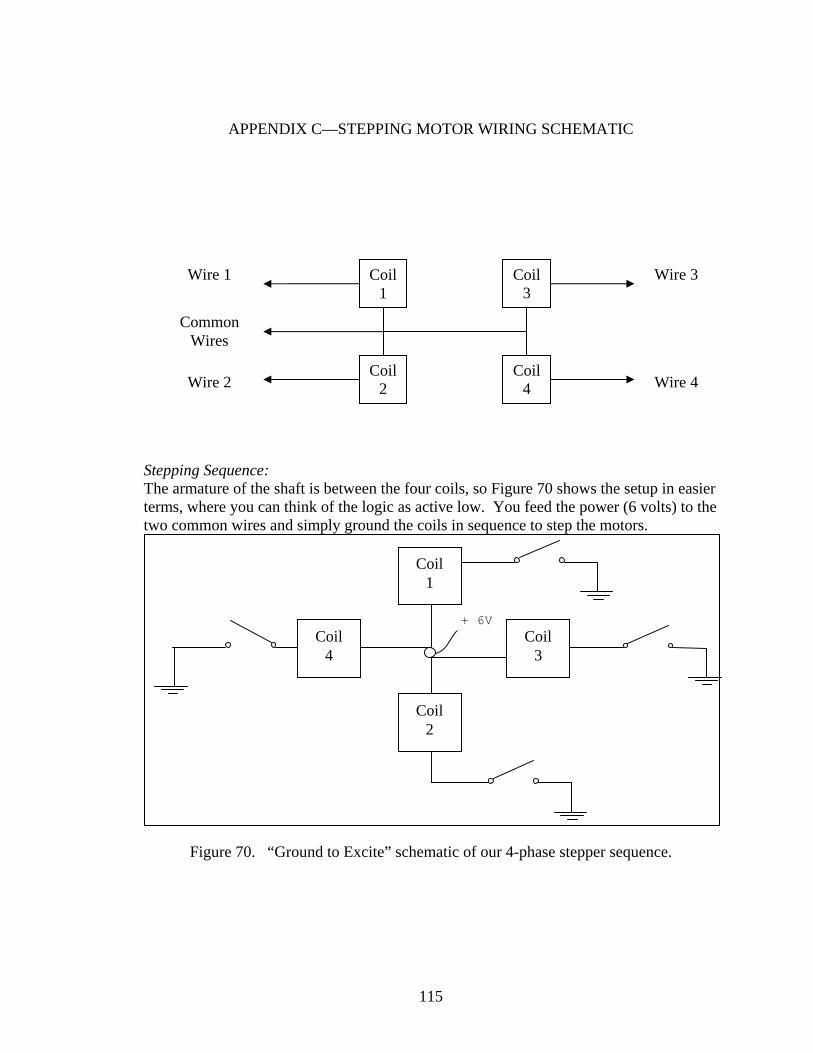
115
APPENDIX C—STEPPING MOTOR WIRING SCHEMATIC
Stepping Sequence: The armature of the shaft is between the four coils, so Figure 70 shows the setup in easier terms, where you can think of the logic as active low. You feed the power (6 volts) to the two common wires and simply ground the coils in sequence to step the motors.
Figure 70. “Ground to Excite” schematic of our 4-phase stepper sequence.
Coil 1
Coil 4
Coil 3
Coil 2
+ 6V
Coil 3
Coil 2
Coil 4
Coil 1
Common Wires
Wire 2
Wire 1 Wire 3
Wire 4
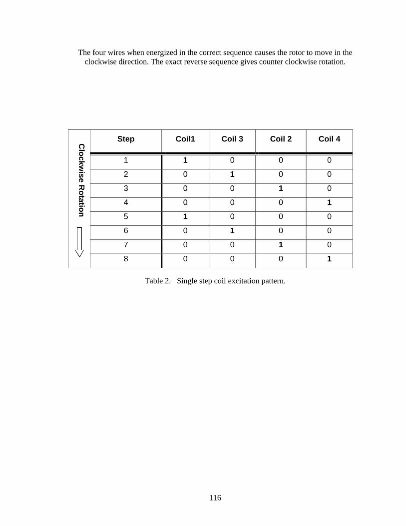
116
The four wires when energized in the correct sequence causes the rotor to move in the clockwise direction. The exact reverse sequence gives counter clockwise rotation.
Step Coil1 Coil 3 Coil 2 Coil 4
1 1 0 0 0
2 0 1 0 0
3 0 0 1 0
4 0 0 0 1
5 1 0 0 0
6 0 1 0 0
7 0 0 1 0
Clockw
ise Rotation
8 0 0 0 1
Table 2. Single step coil excitation pattern.
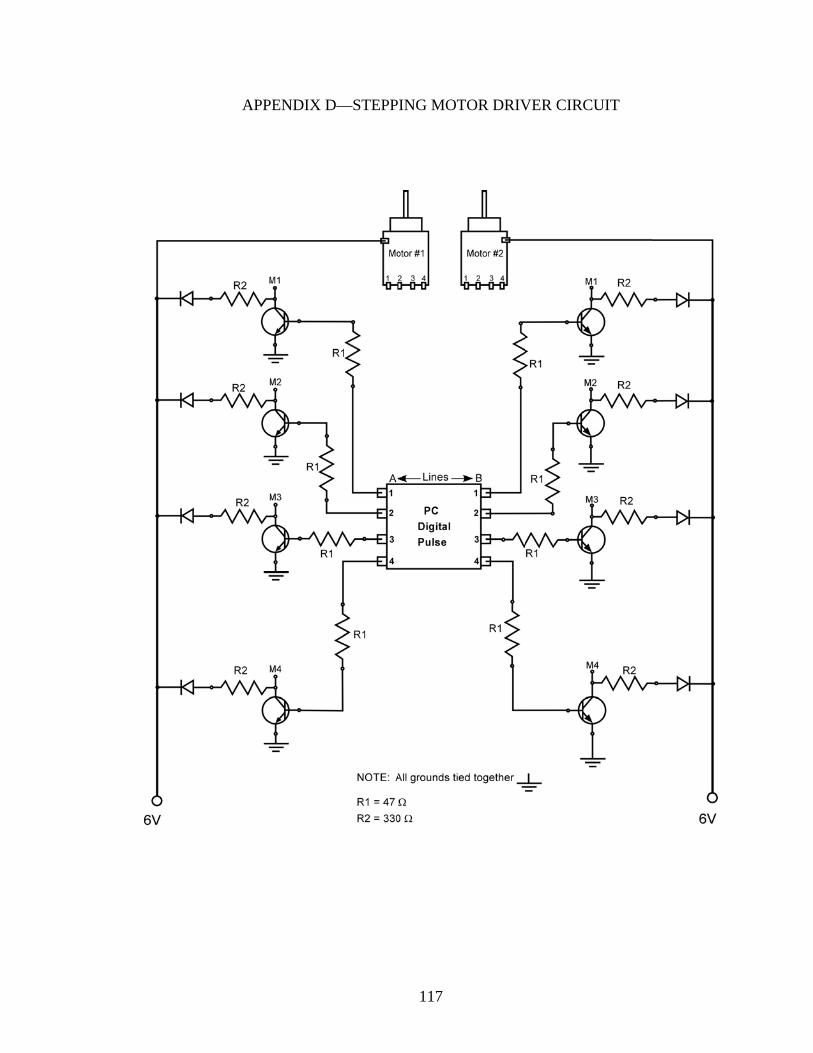
117
APPENDIX D—STEPPING MOTOR DRIVER CIRCUIT
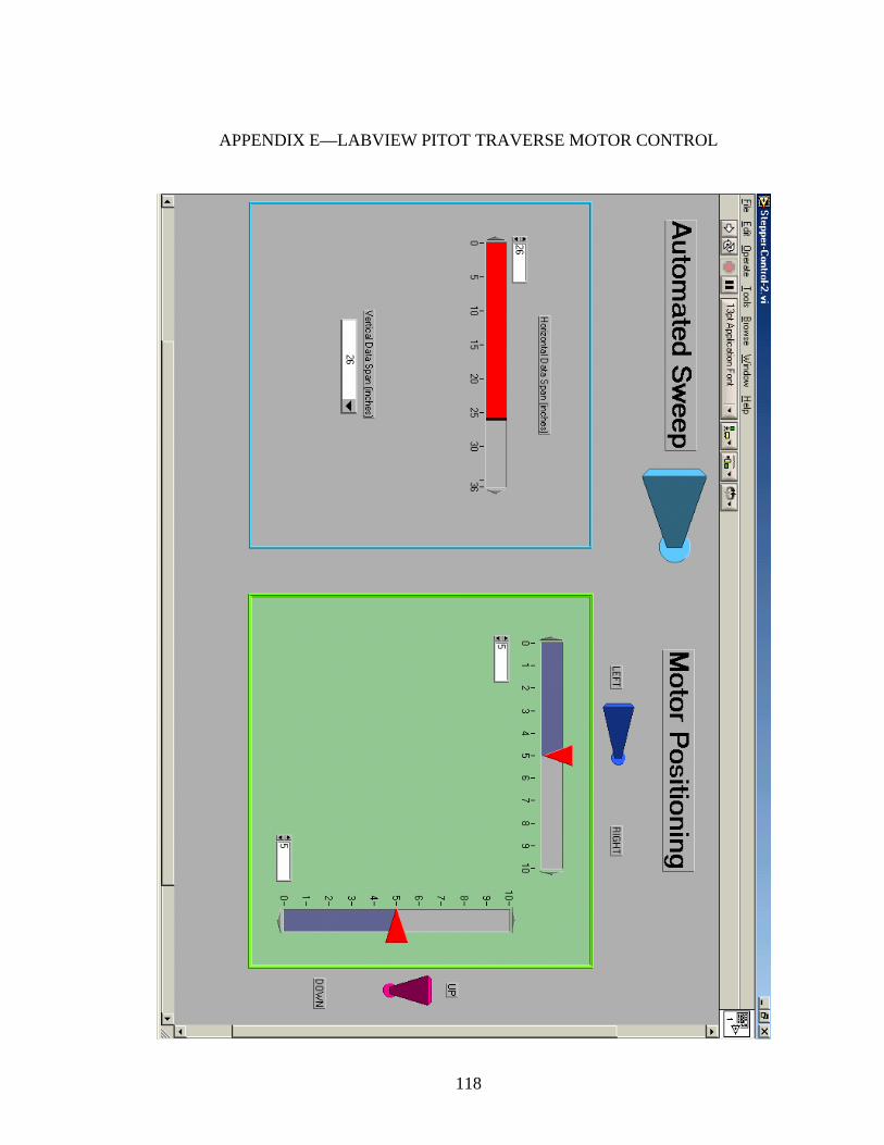
118
APPENDIX E—LABVIEW PITOT TRAVERSE MOTOR CONTROL
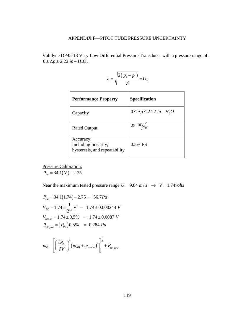
119
APPENDIX F—PITOT TUBE PRESSURE UNCERTAINTY
Validyne DP45-18 Very Low Differential Pressure Transducer with a pressure range of: 20 2.22 p in H O≤ Δ ≤ − .
( )1
1
2 so
p pv U
ρ−
= =
Performance Property Specification
Capacity 20 2.22 p in H O≤ Δ ≤ −
Rated Output mv25 V
Accuracy: Including linearity, hysteresis, and repeatability
0.5% FS
Pressure Calibration:
( )34.1 V 2.75PaP = − Near the maximum tested pressure range 9.84 / 1.74U m s V volts= → =
( )34.1 1.74 2.75 56.7PaP Pa= − =
( )
12
10
11.74 V 1.74 0.000244 2
1.74 0.5% 1.74 0.0087 0.5% 0.284
AD
nonlin
Payaw
V V
V VP P Pa
= ± = ±
= ± = ±
= =
( )1
2 22
10Pa
P AD nonlin yaw
P PV
ω ω ω⎡ ⎤∂⎛ ⎞= + +⎢ ⎥⎜ ⎟∂⎝ ⎠⎢ ⎥⎣ ⎦
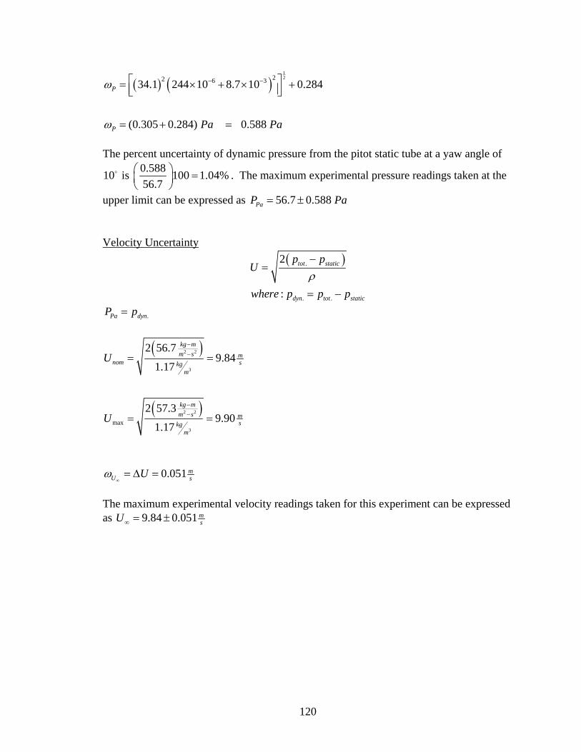
120
( ) ( )1222 6 334.1 244 10 8.7 10 0.284
(0.305 0.284) 0.588
P
P Pa Pa
ω
ω
− −⎡ ⎤= × + × +⎢ ⎥⎣ ⎦
= + =
The percent uncertainty of dynamic pressure from the pitot static tube at a yaw angle of
10 is 0.588 100 1.04%56.7
⎛ ⎞ =⎜ ⎟⎝ ⎠
. The maximum experimental pressure readings taken at the
upper limit can be expressed as 56.7 0.588 PaP Pa= ± Velocity Uncertainty
( ).
. .
2
:
tot static
dyn tot static
p pU
where p p pρ−
=
= −
.Pa dynP p=
( )
( )
2 2
3
2 2
3max
2 56.79.84
1.17
2 57.39.90
1.17
kg mm s m
nom skgm
kg mm s m
skgm
U
U
−−
−−
= =
= =
0.051 m
U sUω∞
= Δ = The maximum experimental velocity readings taken for this experiment can be expressed as 9.84 0.051 m
sU∞ = ±

121
APPENDIX G—MATLAB CROSS-POWER-SPECTRUM M-FILE
%Cross-Power-Spectrum Analysis clear all, close all, clc; SampleRate=500; %A=xlsread('freq__sine_test'); %A=xlsread('freq__1_D0_025'); %A=xlsread('freq__1_D0_0275'); %A=xlsread('freq__1_D0_045'); %A=xlsread('freq__1_D0_06'); %A=xlsread('freq__1_D0_07'); %A=xlsread('freq__1_D0_08'); %A=xlsread('freq__1_D0_09'); %A=xlsread('freq__1_D0_1'); %A=xlsread('freq__1_D0_125'); %A=xlsread('freq__1_D0_14'); %A=xlsread('freq__1_D0_15'); %A=xlsread('freq__1_D0_17'); %A=xlsread('freq__1_D0_185'); %A=xlsread('freq__1_D0_2'); %A=xlsread('freq__1_D0_215'); %A=xlsread('freq__1_D0_23'); %A=xlsread('freq__1_D0_245'); %A=xlsread('freq__1_D0_245-2'); %A=xlsread('cook_d_05-onset'); %A=xlsread('cook_d_06'); %A=xlsread('cook_d_08'); %A=xlsread('cook_d_1'); %A=xlsread('cook_d_12'); %A=xlsread('cook_d_14'); %A=xlsread('cook_d_16'); %A=xlsread('cook_d_18'); %A=xlsread('cook_d_21'); %A=xlsread('cook_d_24'); %A=xlsread('cook_d_27'); %A=xlsread('cook_d_30'); %A=xlsread('cook_d_33'); %A=xlsread('cook_d_36'); %A=xlsread('cook_d_39'); %A=xlsread('cook_d_42'); %A=xlsread('cook_d_45'); A=xlsread('cook_d_48'); x1=A(1:32768,1)'; x2=A(1:32768,2)';
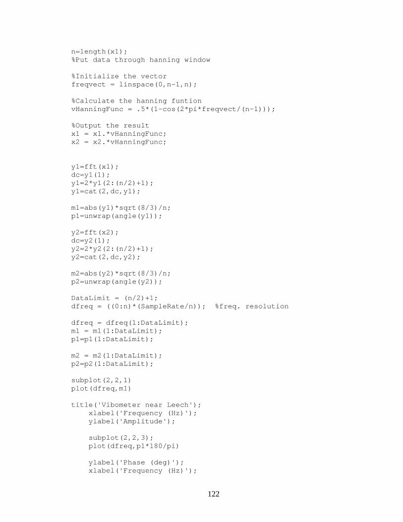
122
n=length(x1); %Put data through hanning window %Initialize the vector freqvect = linspace(0,n-1,n); %Calculate the hanning funtion vHanningFunc = .5*(1-cos(2*pi*freqvect/(n-1))); %Output the result x1 = x1.*vHanningFunc; x2 = x2.*vHanningFunc; y1=fft(x1); dc=y1(1); y1=2*y1(2:(n/2)+1); y1=cat(2,dc,y1); m1=abs(y1)*sqrt(8/3)/n; p1=unwrap(angle(y1)); y2=fft(x2); dc=y2(1); y2=2*y2(2:(n/2)+1); y2=cat(2,dc,y2); m2=abs(y2)*sqrt(8/3)/n; p2=unwrap(angle(y2)); DataLimit = (n/2)+1; dfreq = ((0:n)*(SampleRate/n)); %freq. resolution dfreq = dfreq(1:DataLimit); m1 = m1(1:DataLimit); p1=p1(1:DataLimit); m2 = m2(1:DataLimit); p2=p2(1:DataLimit); subplot(2,2,1) plot(dfreq,m1) title('Vibometer near Leech'); xlabel('Frequency (Hz)'); ylabel('Amplitude'); subplot(2,2,3); plot(dfreq,p1*180/pi) ylabel('Phase (deg)'); xlabel('Frequency (Hz)');
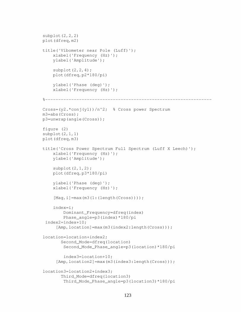
123
subplot(2,2,2) plot(dfreq,m2) title('Vibometer near Pole (Luff)'); xlabel('Frequency (Hz)'); ylabel('Amplitude'); subplot(2,2,4); plot(dfreq,p2*180/pi) ylabel('Phase (deg)'); xlabel('Frequency (Hz)'); %---------------------------------------------------------------- Cross=(y2.*conj(y1))/n^2; % Cross power Spectrum m3=abs(Cross); p3=unwrap(angle(Cross)); figure (2) subplot(2,1,1) plot(dfreq,m3) title('Cross Power Spectrum Full Spectrum (Luff X Leech)'); xlabel('Frequency (Hz)'); ylabel('Amplitude'); subplot(2,1,2); plot(dfreq,p3*180/pi) ylabel('Phase (deg)'); xlabel('Frequency (Hz)'); [Mag,i]=max(m3(1:(length(Cross)))); index=i; Dominant_Frequency=dfreq(index) Phase_angle=p3(index)*180/pi index2=index+10; [Amp,location]=max(m3(index2:length(Cross))); location=location+index2; Second_Mode=dfreq(location) Second_Mode_Phase_angle=p3(location)*180/pi index3=location+10; [Amp,location2]=max(m3(index3:length(Cross))); location3=location2+index3; Third_Mode=dfreq(location3) Third_Mode_Phase_angle=p3(location3)*180/pi

124
index4=location3+10; [Amp,location4]=max(m3(index4:length(Cross))); location5=location4+index4; Fourth_Mode=dfreq(location5) Fourth_Mode_Phase_angle=p3(location5)*180/pi output=[dfreq(index),p3(index)*180/pi,dfreq(location),p3(location)*180/pi,Third_Mode, Third_Mode_Phase_angle,Fourth_Mode,Fourth_Mode_Phase_angle] x1=A(1:32768,1); x2=A(1:32768,2); n=length(x1); avg_x1=mean(x1); avg_x2=mean(x2); max_x1=max(x1); max_x2=max(x2); min_x1=min(x1); min_x2=min(x2); x1=x1.^2; x2=x2.^2; x1=(1/SampleRate).*x1; x2=(1/SampleRate).*x2; x1=sum(x1); x1=(1/(n-1))*x1; x2=sum(x2); x2=(1/(n-1))*x2; rms_x1=sqrt(x1); rms_x2=sqrt(x2) ; output2=[avg_x1,avg_x2,max_x1,max_x2,min_x1,min_x2,rms_x1,rms_x2] figure (3) subplot(2,1,1) plot(dfreq,m3) axis([0 25 0 max(m3)+.0025]) title('Cross Power Spectrum (5.27 m/s)'); xlabel('Frequency (Hz)'); ylabel('Amplitude'); gtext(strcat(' \omega_1=',num2str(dfreq(index)), 'Hz at \phi = ' ,num2str(p3(index)*180/pi), ' deg' )); subplot(2,1,2); plot(dfreq,p3*180/pi) ylabel('Phase (deg)'); xlabel('Frequency (Hz)'); axis([0 25 min(p3)*180/pi-50 max(p3)*180/pi+50]) %-----------------------------------------------
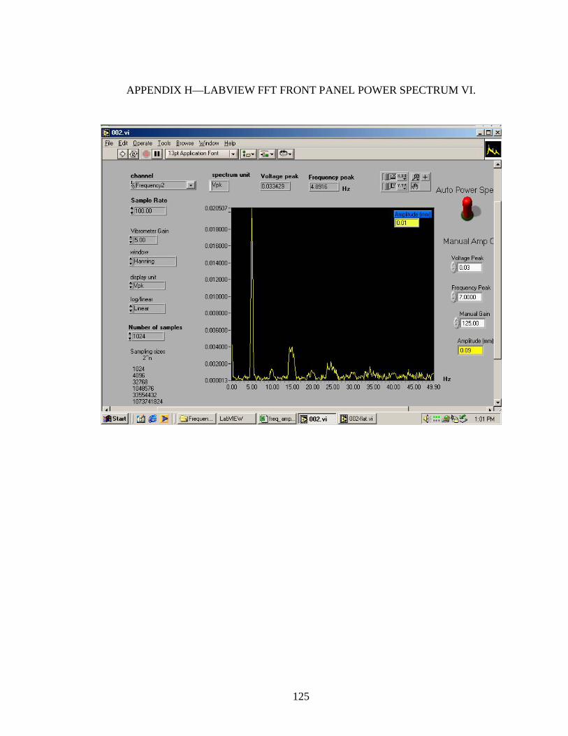
125
APPENDIX H—LABVIEW FFT FRONT PANEL POWER SPECTRUM VI.
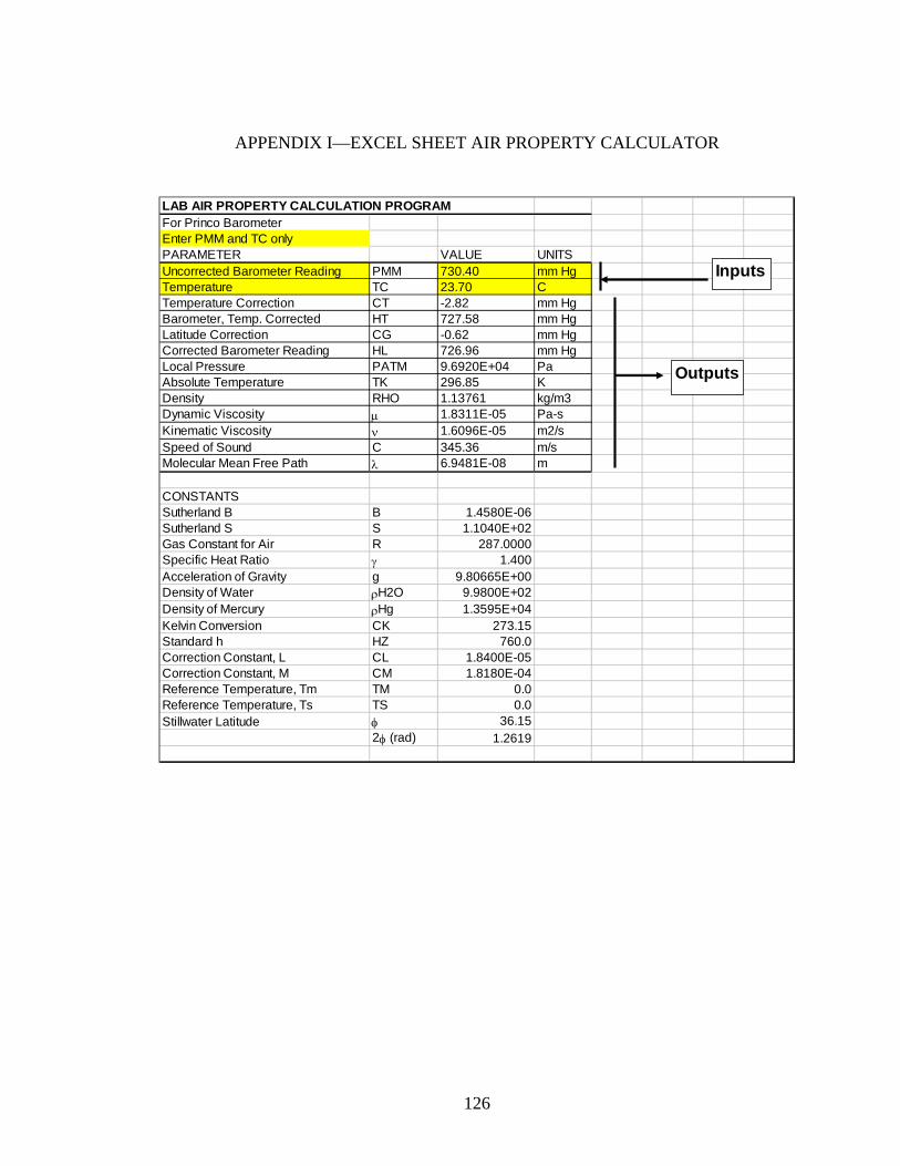
126
APPENDIX I—EXCEL SHEET AIR PROPERTY CALCULATOR
LAB AIR PROPERTY CALCULATION PROGRAMFor Princo BarometerEnter PMM and TC onlyPARAMETER VALUE UNITSUncorrected Barometer Reading PMM 730.40 mm HgTemperature TC 23.70 CTemperature Correction CT -2.82 mm HgBarometer, Temp. Corrected HT 727.58 mm HgLatitude Correction CG -0.62 mm HgCorrected Barometer Reading HL 726.96 mm HgLocal Pressure PATM 9.6920E+04 PaAbsolute Temperature TK 296.85 KDensity RHO 1.13761 kg/m3Dynamic Viscosity μ 1.8311E-05 Pa-sKinematic Viscosity ν 1.6096E-05 m2/sSpeed of Sound C 345.36 m/sMolecular Mean Free Path λ 6.9481E-08 m
CONSTANTSSutherland B B 1.4580E-06Sutherland S S 1.1040E+02Gas Constant for Air R 287.0000Specific Heat Ratio γ 1.400Acceleration of Gravity g 9.80665E+00Density of Water ρH2O 9.9800E+02Density of Mercury ρHg 1.3595E+04Kelvin Conversion CK 273.15Standard h HZ 760.0Correction Constant, L CL 1.8400E-05Correction Constant, M CM 1.8180E-04Reference Temperature, Tm TM 0.0Reference Temperature, Ts TS 0.0Stillwater Latitude φ 36.15
2φ (rad) 1.2619
Inputs
Outputs
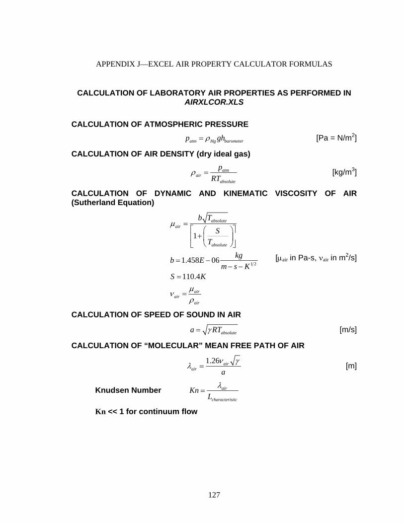
127
APPENDIX J—EXCEL AIR PROPERTY CALCULATOR FORMULAS
CALCULATION OF LABORATORY AIR PROPERTIES AS PERFORMED IN AIRXLCOR.XLS
CALCULATION OF ATMOSPHERIC PRESSURE atm Hg barometerp ghρ= [Pa = N/m2]
CALCULATION OF AIR DENSITY (dry ideal gas)
atmair
absolute
pRT
ρ = [kg/m3]
CALCULATION OF DYNAMIC AND KINEMATIC VISCOSITY OF AIR (Sutherland Equation)
1 2
1
1.458 06
110.4
absoluteair
absolute
airair
air
b T
ST
kgb Em s K
S K
μ
μνρ
=⎡ ⎤⎛ ⎞
+⎢ ⎥⎜ ⎟⎝ ⎠⎣ ⎦
= −− −
=
=
[μair in Pa-s, νair in m2/s]
CALCULATION OF SPEED OF SOUND IN AIR
absolutea RTγ= [m/s]
CALCULATION OF “MOLECULAR” MEAN FREE PATH OF AIR
1.26 airair a
ν γλ = [m]
Knudsen Number air
characteristic
KnL
λ=
Kn << 1 for continuum flow

128
TEMPERATURE CORRECTION OF BAROMETER READING
1 ( ) 1
1 ( )s
t t r rm
L t tC h h hM t t
⎡ ⎤+ −= − = −⎢ ⎥+ −⎣ ⎦
LOCAL GRAVITY CORRECTION OF BAROMETER READING
2980.616[1 0.0026373cos(2 ) 0.0000059cos (2 )] 1980.665g l t tC h h h φ φ⎧ ⎫= − = − + −⎨ ⎬
⎩ ⎭
WHERE: hl = Local Station Pressure Reading
h0 = Standard Pressure Reading at Sea Level
hr = Uncorrected Barometer Reading
ht = Temperature Corrected Barometer Reading
t = Temperature
φ = Latitude (Stillwater Latitude = 36.15 degrees)
Parameter SI English
h0 760 mm 29.921 in. L 0.0000184 m/m °C 0.0000102 in./in. °F M 0.0001818 m3/m3
°C 0.0001010 in.3/in.3 °F tm 0 °C 32 °F ts 0 °C 62 °F g 9.806650 m/s2
ρHg 13.595 x 10³ kg/m3 LOCAL ATMOSPHERIC PRESSURE
atm Hg lp ghρ=
REFERENCE “Instruction Booklet for Use with Princo Fortin Type Mercurial Barometers,” Princo Instruments, Inc., Southampton, Pa., 1983.
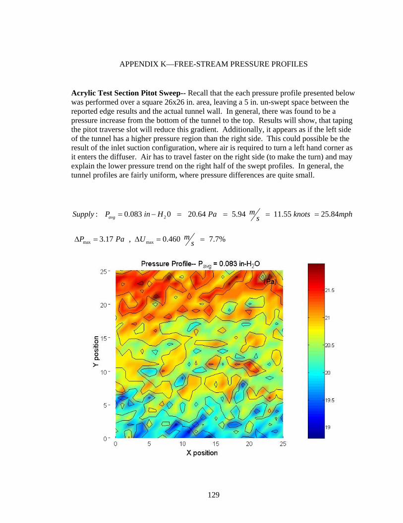
129
APPENDIX K—FREE-STREAM PRESSURE PROFILES
Acrylic Test Section Pitot Sweep-- Recall that the each pressure profile presented below was performed over a square 26x26 in. area, leaving a 5 in. un-swept space between the reported edge results and the actual tunnel wall. In general, there was found to be a pressure increase from the bottom of the tunnel to the top. Results will show, that taping the pitot traverse slot will reduce this gradient. Additionally, it appears as if the left side of the tunnel has a higher pressure region than the right side. This could possible be the result of the inlet suction configuration, where air is required to turn a left hand corner as it enters the diffuser. Air has to travel faster on the right side (to make the turn) and may explain the lower pressure trend on the right half of the swept profiles. In general, the tunnel profiles are fairly uniform, where pressure differences are quite small.
2: 0.083 0 20.64 5.94 11.55 25.84avgmSupply P in H Pa knots mphs= − = = = =
max max 3.17 , 0.460 7.7%mP Pa U sΔ = Δ = =
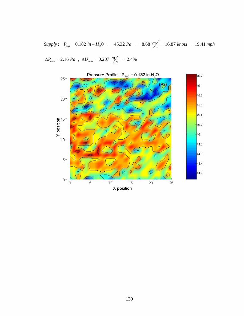
130
2: 0.182 0 45.32 8.68 16.87 19.41 avgmSupply P in H Pa knots mphs= − = = = =
max max 2.16 , 0.207 2.4%mP Pa U sΔ = Δ = =
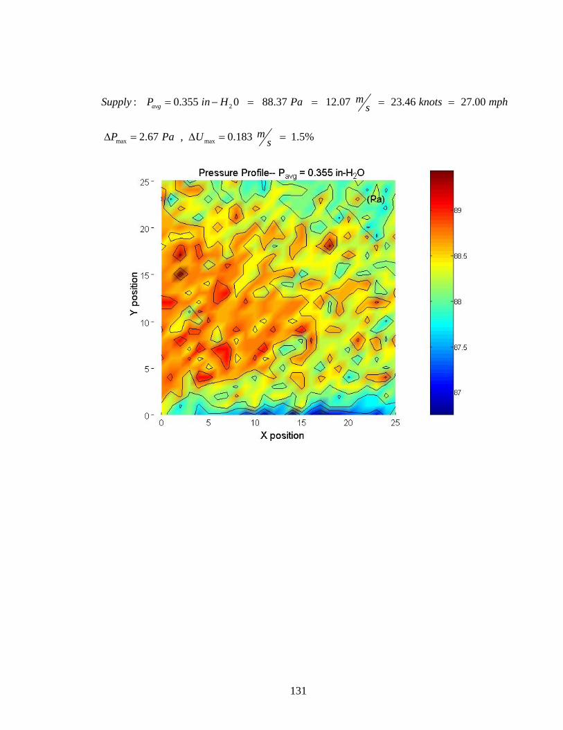
131
2: 0.355 0 88.37 12.07 23.46 27.00 avgmSupply P in H Pa knots mphs= − = = = =
max max 2.67 , 0.183 1.5%mP Pa U sΔ = Δ = =
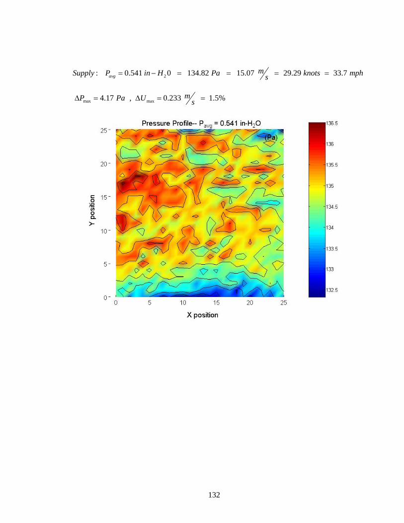
132
2: 0.541 0 134.82 15.07 29.29 33.7 avgmSupply P in H Pa knots mphs= − = = = =
max max 4.17 , 0.233 1.5%mP Pa U sΔ = Δ = =
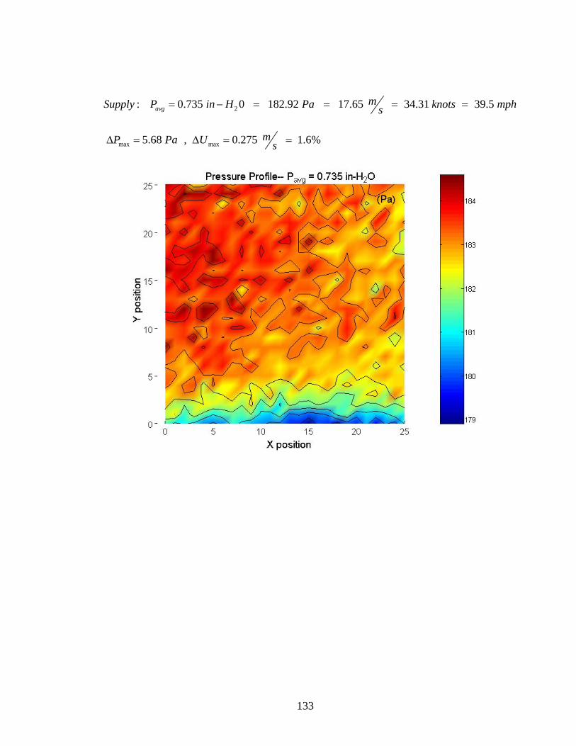
133
2: 0.735 0 182.92 17.65 34.31 39.5 avgmSupply P in H Pa knots mphs= − = = = =
max max 5.68 , 0.275 1.6%mP Pa U sΔ = Δ = =
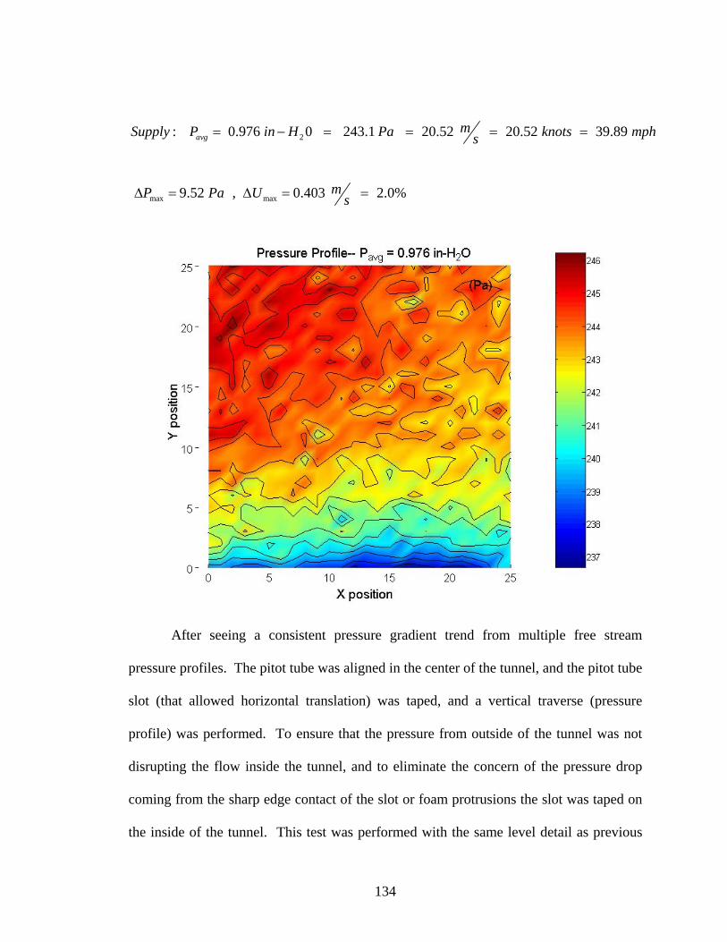
134
2: 0.976 0 243.1 20.52 20.52 39.89 avgmSupply P in H Pa knots mphs= − = = = =
max max 9.52 , 0.403 2.0%mP Pa U sΔ = Δ = =
After seeing a consistent pressure gradient trend from multiple free stream
pressure profiles. The pitot tube was aligned in the center of the tunnel, and the pitot tube
slot (that allowed horizontal translation) was taped, and a vertical traverse (pressure
profile) was performed. To ensure that the pressure from outside of the tunnel was not
disrupting the flow inside the tunnel, and to eliminate the concern of the pressure drop
coming from the sharp edge contact of the slot or foam protrusions the slot was taped on
the inside of the tunnel. This test was performed with the same level detail as previous
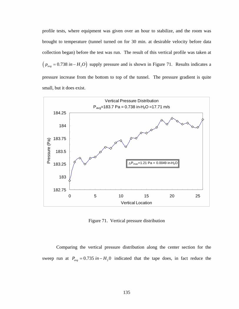
135
profile tests, where equipment was given over an hour to stabilize, and the room was
brought to temperature (tunnel turned on for 30 min. at desirable velocity before data
collection began) before the test was run. The result of this vertical profile was taken at
( )20.738 avgp in H O= − supply pressure and is shown in Figure 71. Results indicates a
pressure increase from the bottom to top of the tunnel. The pressure gradient is quite
small, but it does exist.
Vertical Pressure DistributionPavg=183.7 Pa = 0.738 in-H2O =17.71 m/s
182.75
183
183.25
183.5
183.75
184
184.25
0 5 10 15 20 25Vertical Location
Pre
ssur
e (P
a)
ΔPmax=1.21 Pa = 0.0049 in-H2O
Figure 71. Vertical pressure distribution
Comparing the vertical pressure distribution along the center section for the
sweep run at 20.735 0avgP in H= − indicated that the tape does, in fact reduce the
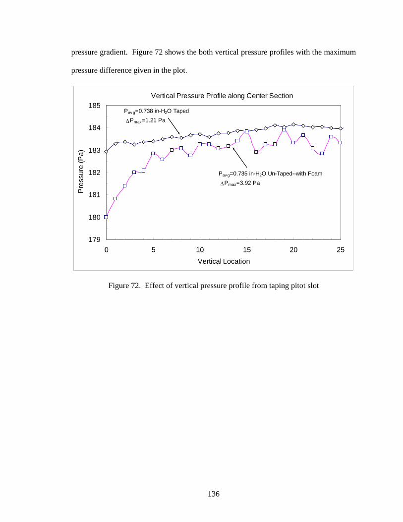
136
pressure gradient. Figure 72 shows the both vertical pressure profiles with the maximum
pressure difference given in the plot.
Vertical Pressure Profile along Center Section
179
180
181
182
183
184
185
0 5 10 15 20 25Vertical Location
Pre
ssur
e (P
a)
Pav g=0.738 in-H2O Taped ΔPmax=1.21 Pa
Pav g=0.735 in-H2O Un-Taped--with Foam ΔPmax=3.92 Pa
Figure 72. Effect of vertical pressure profile from taping pitot slot

VITA
Adam Martin
Candidate for the Degree of
Master of Science Thesis:
EXPERIMENTAL STUDY OF DRAG FROM A FLUTTERING FLAG Major Field: Mechanical Engineering Biographical: Personal Data:
Born in Rapid City, South Dakota, On February 15, 1981, the son of Jeff and Debbie Martin.
Education:
Completed Bachelor of Science degree in Mechanical Engineering Technology from Oklahoma State University, Stillwater, Oklahoma in May 2003. Completed the requirements for a Master of Science degree with a major in Mechanical Engineering at Oklahoma State University in May 2006.
Professional Experience:
Graduate Research Assistant\Teaching Assistant, School of Mechanical and Aerospace Engineering, Oklahoma State University, 2001 to 2006; Honda Research & Development Americas, Summer 2005 Co-op, Vehicle Strength and Simulation; Halliburton Energy Services, Summer 2003 Intern, Mechanical Surface/Reliability Division.

Name: Adam Martin Date of Degree: May, 2006 Institution: Oklahoma State University Location: Stillwater, Oklahoma Title of Study: EXPERIMENTAL STUDY OF DRAG FROM A
FLUTTERING FLAG. Pages in Study: 136 Candidate for the Degree of Master of Science Major Field: Mechanical Engineering Scope and Method of Study:
The purpose of this study is to quantify the magnitude of induced drag force that results from a flexible material (flag) fluttering in air stream versus a stiff panel vane with identical dimensions. Wind tunnel experiments were performed to assess component lift and drag forces on both flexible and rigid vanes. Furthermore, a qualitative and quantitative analysis describing flutter modes are supported from waveform data including: frequency, phase, wavelength, and amplitude.
Findings and Conclusions:
As a result of flutter motion, centrifugal forces induce in-plane tension in the fabric. This tension acts to “flatten” the flag thereby opposing the fluid pressure forces which generate the out-of-plane curvature (motion). This dynamically induced tension is felt at the attachment point as increased drag force, above and beyond the magnitude of skin friction drag. It has been shown experimentally that the time-averaged drag depends only on the square of the velocity amplitude and the mass of the fluttering specimen. Experiments suggest that large centrifugal forces, because of large fabric curvature and low material stiffness can generate elevated drag over that of heavier, stiffer materials with identical dimensions. Furthermore, high speed photo data suggests flutter amplitudes are reduced at high wind velocities due to the induced in-plane tension. Additionally the makeup of flutter oscillations in a flexible flag were proven to consist of both traveling and standing waves. Standing wave ratio (SWR) approximations from superimposed photo data suggests an underlying dominance of traveling waves comprising the flutter motion.
ADVISER’S APPROVAL: Peter M. Moretti