EXISTENCE, POSITIVITY AND CONTRACTIVITY FOR QUANTUM ... · 0. Introduction The quantum stochastic...

EXISTENCE, POSITIVITY AND CONTRACTIVITYFOR QUANTUM STOCHASTIC FLOWSWITH INFINITE DIMENSIONAL NOISE

J MARTIN LINDSAY AND STEPHEN J WILLS

Abstract. Quantum stochastic differential equations of the form

dkt = kt ◦ θαβ dΛβ

α(t)

govern stochastic flows on a C∗-algebra A. We analyse this class of equation inwhich the matrix of fundamental quantum stochastic integrators Λ is infinite

dimensional, and the coefficient matrix θ consists of bounded linear operatorson A. Weak and strong forms of solution are distinguished, and a range ofregularity conditions on the mapping matrix θ are considered, for investigating

existence and uniqueness of solutions. Necessary and sufficient conditions onθ are determined, for any sufficiently regular weak solution k to be completelypositive. The further conditions on θ for k to also be a contraction process

are found; and when A is a von Neumann algebra and the components of θare normal, these in turn imply sufficient regularity for the equation to havea strong solution. Weakly multiplicative and ∗-homomorphic solutions and

their generators are also investigated. We then consider the right and leftHudson-Parthasarathy equations:

dXt = F αβ Xt dΛβ

α(t), dYt = YtFαβ dΛβ

α(t),

in which F is a matrix of bounded Hilbert space operators. Their solutions

are interchanged by a time reversal operation on processes. The analysis of

quantum stochastic flows is applied to obtain characterisations of the genera-tors F of contraction, isometry and coisometry processes. In particular weak

solutions that are contraction processes are shown to have bounded generators,

and to be necessarily strong solutions.

0. Introduction

The quantum stochastic differential equation (QSDE)

dkt = kt ◦ θαβ dΛβα(t), (0.1)

in which θ = [θαβ ] is a matrix of linear maps on a C∗-algebra and Λ = [Λαβ ] is thematrix of fundamental noise processes of quantum stochastic calculus ([Par],[Mey]),has been studied from a variety of points of view. Hudson and Evans sought unital∗-homomorphic solutions, and called these quantum diffusions ([Hud],[Eva],[EvH]);Mohari and Sinha extended this work by allowing the noise and mapping matrix tobe infinite dimensional ([MoS],[Moh]); and, extending the original work of Hudsonand Parthasarathy ([HuP]), Fagnola and Mohari studied isometric, coisometric andcontractive solutions of the related QSDE’s

dXt = Fαβ Xt dΛβα(t), (0.2)

dYt = YtFαβ dΛ

βα(t), (0.3)

1991 Mathematics Subject Classification. 81S25,60H20,46L50.Key words and phrases. Quantum stochastic, completely positive, completely bounded, sto-

chastic flows, quantum Markov semigroup, quantum diffusion.

1

2 J MARTIN LINDSAY AND STEPHEN J WILLS

in which F = [Fαβ ] is a matrix of Hilbert space operators ([Fag],[Moh]). Lindsay andParthasarathy gave a comprehensive analysis of completely positive (CP) solutions,and completely positive contraction solutions of (0.1) for finite dimensional noiseand mapping matrix ([LP1,2]), and applied their results to QSDE’s of the form(0.2) whose solutions provide CP flows by conjugation:

kt(a) = X∗t aXt. (0.4)

One motivation for extending the study of (0.1) from quantum diffusions to CPflows was to develop an approach to Belavkin’s quantum filtering theory ([Be1]) inwhich processes of the form (0.4) arise, by viewing these as “inner” CP flows. Asstated in [LP1] the broader framework of completely positive flows is required inorder to formulate a quantum theory of measure-valued diffusions — quantum dif-fusions corresponding to stochastic flows of diffeomorphisms. Another motivationwas to see Evans and Hudson’s characterisation of the generators of quantum diffu-sions, and Lindblad’s characterisation of quantum dynamical semigroup generators([Lin],[GKS]), and its subsequent refinements ([ChE]), from a common perspective.

In the present paper we analyse (0.1) in the infinite dimensional case. Whereaseach map θαβ is assumed to be bounded, the whole matrix θ is not assumed to definea bounded map. Indeed the interplay between boundedness of θ, regularity condi-tions on θ and the complete positivity and contractivity of solutions is central toour analysis. For us the standing hypothesis is the existence of a weak solution sat-isfying a mild regularity condition; such solutions are unique and necessarily linear.The set of matrices θ for which the solution is CP (respectively, a CP contraction,unital, weakly multiplicative, or ∗-homomorphic process) is characterised. Whenk is a CP contraction process, θ is shown to be completely bounded. A regularitycondition on θ ensures the existence of a strong solution, and also that the standinghypothesis is satisfied. It is shown that when θ is completely bounded and A is avon Neumann algebra, ultraweak continuity of θ is equivalent to a stronger formof regularity devised and exploited by Mohari and Sinha. We thereby obtain anexistence theorem for normal CP contraction flows on a von Neumann algebra. Theresults on the QSDE (0.1) yield a straightforward and illuminating approach to theQSDE’s (0.2) and (0.3), and are applied to the questions of existence and unique-ness of solutions, and determining when the solutions are contraction, isometry orcoisometry processes, unifying and extending the results of Fagnola and Mohari([Fag],[Moh]). The interchange of solutions of (0.2) and (0.3) by time reversal isgiven a very simple explanation. The central tool of our approach is the semigrouprepresentation of solutions of (0.1).

The structure of the paper is as follows. Section 1 contains the basic definitionsand results on infinite matrices of bounded Hilbert space operators, and of boundedlinear maps on a C∗-algebra, and establishes the equivalence of ultraweak continu-ity and Mohari-Sinha regularity for completely bounded mapping matrices on a vonNeumann algebra (Proposition 1.3). Section 2 gives a review of quantum stochasticintegration with infinite dimensional noise in a form best suited to our purposes.Weak and strong solutions of (0.1) are considered in Section 3. By choice of domain,the uniqueness of weakly regular weak solutions follows as in the case of finite dimen-sional noise, as does its representation in terms of the collection of one-parametersemigroups on the algebra whose generators are a linear combination of the θαβ .Following Meyer, we give a refinement of the Mohari-Sinha existence theorem, butwith simplified proof, in Theorem 3.3. In Section 4 the generators of CP flows arecharacterised. Unlike the case of finite dimensional noise, here the existence of theflow must be assumed. In Section 5 the generators of CP contraction flows are char-acterised, again under the assumption of existence. It is shown that the generatorsof such flows are necessarily completely bounded (Theorem 5.2). Combined with

QUANTUM STOCHASTIC FLOWS 3

Proposition 1.3 mentioned above, this gives an existence theorem for CP contrac-tion flows on a von Neumann algebra (Theorem 5.3). In Section 6 we specialise to∗-homomorphic and weakly multiplicative flows and their generators. An existencetheorem for weakly multiplicative flows is given, and a converse is proved, show-ing necessity of the weak multiplicativity conditions on the generator. In the finalsection the above results are applied to the right and left Hudson-Parthasarathyequations, (0.2) and (0.3). Specifically we deduce uniqueness, semigroup represen-tations, and the Mohari-Sinha existence theorem for the two QSDE’s, from thecorresponding results for the flow equation (Theorem 7.1), yielding a transparentdemonstration that solutions of (0.2) and (0.3) are interchanged by time reversal(Theorem 7.2). Conjugation by solutions of the right H-P equation (0.2) is shownto resonate perfectly with the corresponding flow equation (Theorem 7.4). Finallythe operator matrices F for which the H-P equations (0.2) and (0.3) have weaksolutions which are contraction (respectively isometry or coisometry) processes, arecharacterised (Theorem 7.5 and Proposition 7.6) — a key point being that thegenerating operator matrices are necessarily bounded.

The results here build on work of Hudson, Parthasarathy, Evans, Mohari, Sinha,Meyer and Lindsay, and complement the work of Journe, Fagnola and Belavkin.In conjunction with [LP2] the paper is almost self-contained, however the books[Par], [Mey] and [Bia] are recommended company for the nonspecialist reader. Thecharacterisation of CP flow generators was reported in the conference proceed-ings [LW1], where a version of the existence result Theorem 5.3 was proved understronger hypotheses (complete positivity and unitality, rather than contractivity).A preliminary account of most of the present results may be found in the PhDthesis [W]. Results characterising the generators of a large class of CP form-valuedflows have also been obtained by Belavkin ([Be2,3]). In a very recent preprintGoswami and Sinha have obtained an existence theorem for ∗-homomorphic flowson a von Neumann algebra, in a coordinate-free quantum stochastic calculus usingHilbert W ∗-modules ([GoS]). Their assumptions amount to the coefficient matrixbeing ultraweakly continuous, and taking the form necessary for a ∗-homomorphicsolution. Free from coordinates they make no separability assumption on the noisedimension space, and indeed exploit this freedom to describe a natural dilation forany quantum dynamical semigroup on a von Neumann algebra having a boundedgenerator. A converse question to the main concern of the present paper is thealgebraic characterisation of the collection of processes on an algebra which satisfya QSDE of the form (0.1). This is analysed in a sister paper [LW2], where thesemigroup representation again plays an important role.

1. Infinite Matrices

In this section we collect together some observations on infinite matrices ofHilbert space operators and C∗-algebra maps. This will provide us with the basictools for dealing with the infinite dimensional aspects of the analysis of QSDE’s ofthe form (0.1), (0.2) and (0.3). We also introduce our basic conventions and nota-tions. A Hilbert space k, called the noise dimension space; another Hilbert spaceh, called the initial space; and a unital C∗-algebra A, acting on h, called the initialalgebra are all fixed throughout the paper. Sometimes A will be further assumed tobe a von Neumann algebra; this will always be indicated. Moreover here the noisedimension space k is infinite dimensional and separable, with fixed orthonormalbasis η = (ei)i≥1, and this basis is extended to a basis (eγ)γ≥0 of k := C ⊕ k, byputting e0 = 1 ∈ C.

General Conventions. Algebraic tensor products are denoted �, the symbol ⊗being reserved for Hilbert space and von Neumann algebra tensor products. The


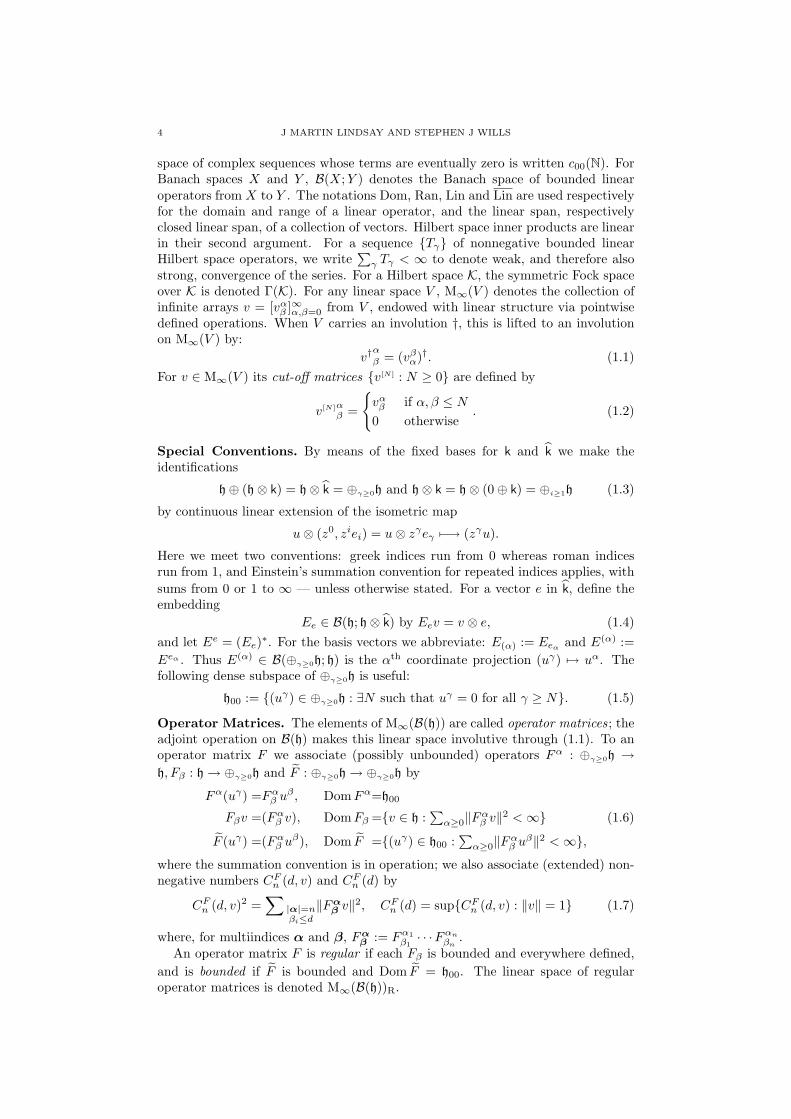
space of complex sequences whose terms are eventually zero is written c00(N). ForBanach spaces X and Y , B(X;Y ) denotes the Banach space of bounded linearoperators from X to Y . The notations Dom, Ran, Lin and Lin are used respectivelyfor the domain and range of a linear operator, and the linear span, respectivelyclosed linear span, of a collection of vectors. Hilbert space inner products are linearin their second argument. For a sequence {Tγ} of nonnegative bounded linearHilbert space operators, we write

∑γ Tγ < ∞ to denote weak, and therefore also

strong, convergence of the series. For a Hilbert space K, the symmetric Fock spaceover K is denoted Γ(K). For any linear space V , M∞(V ) denotes the collection ofinfinite arrays v = [vαβ ]∞α,β=0 from V , endowed with linear structure via pointwisedefined operations. When V carries an involution †, this is lifted to an involutionon M∞(V ) by:

v†α

β = (vβα)†. (1.1)For v ∈ M∞(V ) its cut-off matrices {v[N] : N ≥ 0} are defined by

v[N]αβ =

{vαβ if α, β ≤ N

0 otherwise. (1.2)

Special Conventions. By means of the fixed bases for k and k we make theidentifications

h⊕ (h⊗ k) = h⊗ k = ⊕γ≥0h and h⊗ k = h⊗ (0⊕ k) = ⊕i≥1h (1.3)

by continuous linear extension of the isometric map

u⊗ (z0, ziei) = u⊗ zγeγ 7−→ (zγu).

Here we meet two conventions: greek indices run from 0 whereas roman indicesrun from 1, and Einstein’s summation convention for repeated indices applies, withsums from 0 or 1 to ∞ — unless otherwise stated. For a vector e in k, define theembedding

Ee ∈ B(h; h⊗ k) by Eev = v ⊗ e, (1.4)and let Ee = (Ee)∗. For the basis vectors we abbreviate: E(α) := Eeα and E(α) :=Eeα . Thus E(α) ∈ B(⊕γ≥0h; h) is the αth coordinate projection (uγ) 7→ uα. Thefollowing dense subspace of ⊕γ≥0h is useful:

h00 := {(uγ) ∈ ⊕γ≥0h : ∃N such that uγ = 0 for all γ ≥ N}. (1.5)

Operator Matrices. The elements of M∞(B(h)) are called operator matrices; theadjoint operation on B(h) makes this linear space involutive through (1.1). To anoperator matrix F we associate (possibly unbounded) operators Fα : ⊕γ≥0h →h, Fβ : h → ⊕γ≥0h and F : ⊕γ≥0h → ⊕γ≥0h by

Fα(uγ) =Fαβ uβ , DomFα=h00

Fβv =(Fαβ v), DomFβ ={v ∈ h :∑α≥0‖Fαβ v‖2 <∞} (1.6)

F (uγ) =(Fαβ uβ), Dom F ={(uγ) ∈ h00 :

∑α≥0‖Fαβ uβ‖2 <∞},

where the summation convention is in operation; we also associate (extended) non-negative numbers CFn (d, v) and CFn (d) by

CFn (d, v)2 =∑

|α|=nβi≤d

‖Fαβ v‖2, CFn (d) = sup{CFn (d, v) : ‖v‖ = 1} (1.7)

where, for multiindices α and β, Fαβ := Fα1

β1· · ·Fαn

βn.

An operator matrix F is regular if each Fβ is bounded and everywhere defined,and is bounded if F is bounded and Dom F = h00. The linear space of regularoperator matrices is denoted M∞(B(h))R.


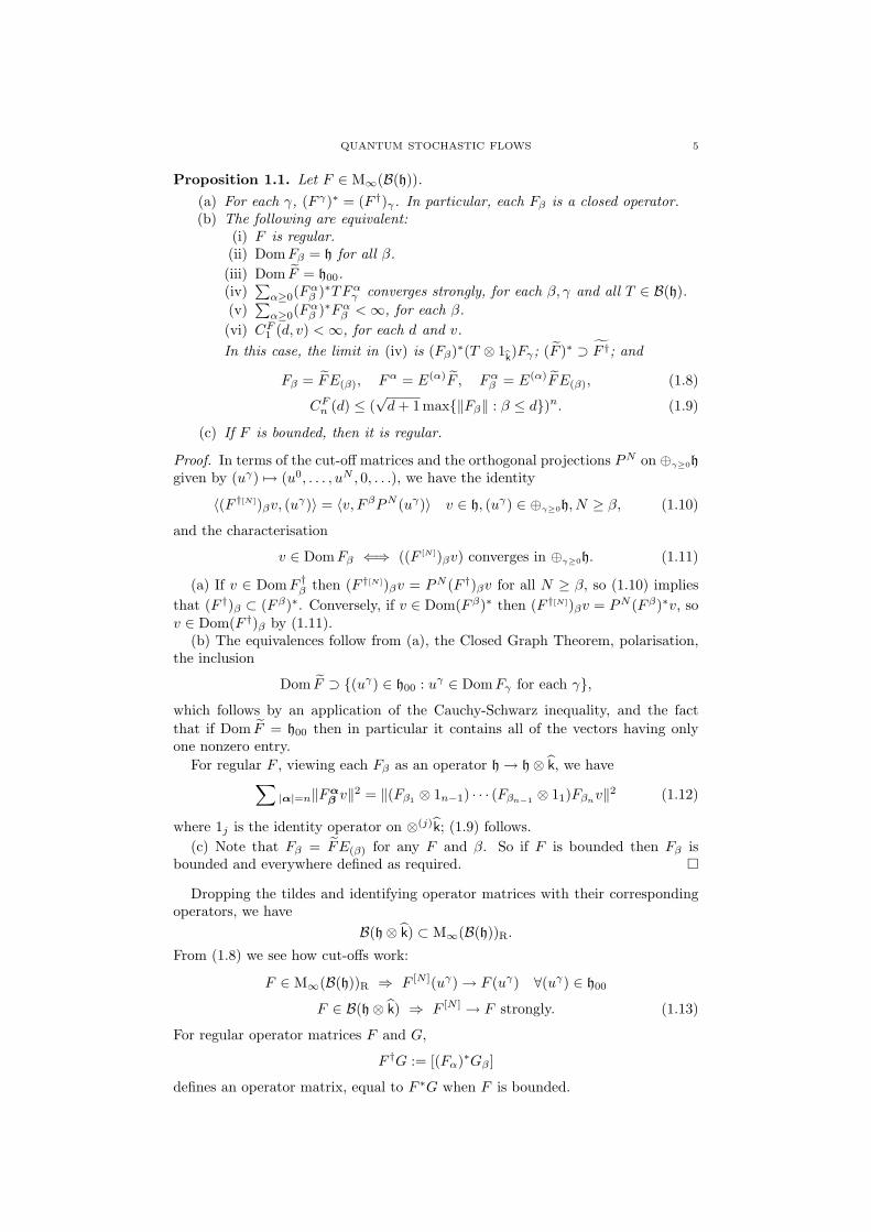
Proposition 1.1. Let F ∈ M∞(B(h)).(a) For each γ, (F γ)∗ = (F †)γ . In particular, each Fβ is a closed operator.(b) The following are equivalent:

(i) F is regular.(ii) DomFβ = h for all β.(iii) Dom F = h00.(iv)

∑α≥0(F

αβ )∗TFαγ converges strongly, for each β, γ and all T ∈ B(h).

(v)∑α≥0(F

αβ )∗Fαβ <∞, for each β.

(vi) CF1 (d, v) <∞, for each d and v.In this case, the limit in (iv) is (Fβ)∗(T ⊗ 1k)Fγ ; (F )∗ ⊃ F †; and

Fβ = FE(β), Fα = E(α)F , Fαβ = E(α)FE(β), (1.8)

CFn (d) ≤ (√d+ 1 max{‖Fβ‖ : β ≤ d})n. (1.9)

(c) If F is bounded, then it is regular.

Proof. In terms of the cut-off matrices and the orthogonal projections PN on ⊕γ≥0hgiven by (uγ) 7→ (u0, . . . , uN , 0, . . .), we have the identity

〈(F †[N])βv, (uγ)〉 = 〈v, F βPN (uγ)〉 v ∈ h, (uγ) ∈ ⊕γ≥0h, N ≥ β, (1.10)

and the characterisation

v ∈ DomFβ ⇐⇒ ((F [N])βv) converges in ⊕γ≥0h. (1.11)

(a) If v ∈ DomF †β then (F †[N])βv = PN (F †)βv for all N ≥ β, so (1.10) impliesthat (F †)β ⊂ (F β)∗. Conversely, if v ∈ Dom(F β)∗ then (F †[N])βv = PN (F β)∗v, sov ∈ Dom(F †)β by (1.11).

(b) The equivalences follow from (a), the Closed Graph Theorem, polarisation,the inclusion

Dom F ⊃ {(uγ) ∈ h00 : uγ ∈ DomFγ for each γ},

which follows by an application of the Cauchy-Schwarz inequality, and the factthat if Dom F = h00 then in particular it contains all of the vectors having onlyone nonzero entry.

For regular F , viewing each Fβ as an operator h → h⊗ k, we have∑|α|=n‖Fα

β v‖2 = ‖(Fβ1 ⊗ 1n−1) · · · (Fβn−1 ⊗ 11)Fβnv‖2 (1.12)

where 1j is the identity operator on ⊗(j)k; (1.9) follows.(c) Note that Fβ = FE(β) for any F and β. So if F is bounded then Fβ is

bounded and everywhere defined as required. �

Dropping the tildes and identifying operator matrices with their correspondingoperators, we have

B(h⊗ k) ⊂ M∞(B(h))R.

From (1.8) we see how cut-offs work:

F ∈ M∞(B(h))R ⇒ F [N ](uγ) → F (uγ) ∀(uγ) ∈ h00

F ∈ B(h⊗ k) ⇒ F [N ] → F strongly. (1.13)

For regular operator matrices F and G,

F †G := [(Fα)∗Gβ ]

defines an operator matrix, equal to F ∗G when F is bounded.


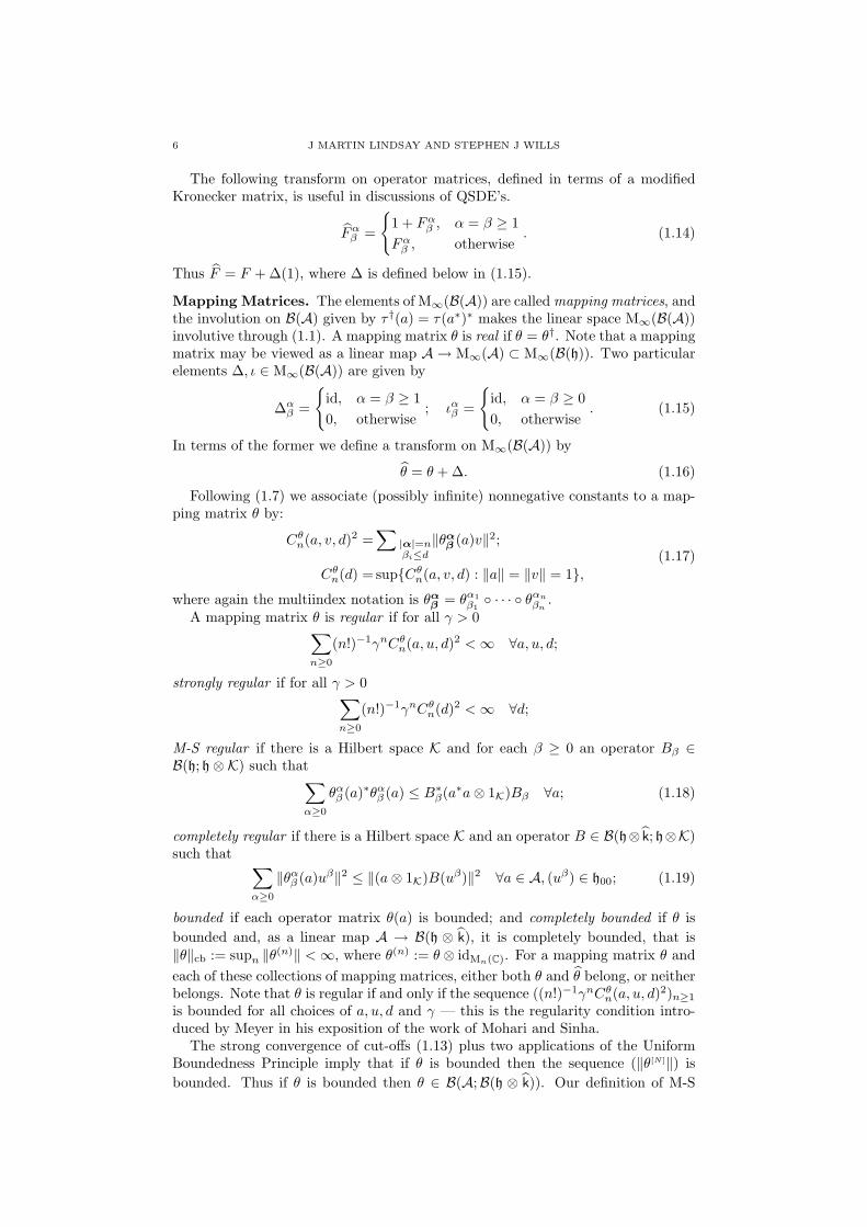
The following transform on operator matrices, defined in terms of a modifiedKronecker matrix, is useful in discussions of QSDE’s.

Fαβ =

{1 + Fαβ , α = β ≥ 1Fαβ , otherwise

. (1.14)

Thus F = F + ∆(1), where ∆ is defined below in (1.15).

Mapping Matrices. The elements of M∞(B(A)) are called mapping matrices, andthe involution on B(A) given by τ †(a) = τ(a∗)∗ makes the linear space M∞(B(A))involutive through (1.1). A mapping matrix θ is real if θ = θ†. Note that a mappingmatrix may be viewed as a linear map A → M∞(A) ⊂ M∞(B(h)). Two particularelements ∆, ι ∈ M∞(B(A)) are given by

∆αβ =

{id, α = β ≥ 10, otherwise

; ιαβ =

{id, α = β ≥ 00, otherwise

. (1.15)

In terms of the former we define a transform on M∞(B(A)) by

θ = θ + ∆. (1.16)

Following (1.7) we associate (possibly infinite) nonnegative constants to a map-ping matrix θ by:

Cθn(a, v, d)2 =

∑|α|=nβi≤d

‖θαβ (a)v‖2;

Cθn(d) = sup{Cθn(a, v, d) : ‖a‖ = ‖v‖ = 1},(1.17)

where again the multiindex notation is θαβ = θα1

β1◦ · · · ◦ θαn

βn.

A mapping matrix θ is regular if for all γ > 0∑n≥0

(n!)−1γnCθn(a, u, d)2 <∞ ∀a, u, d;

strongly regular if for all γ > 0∑n≥0

(n!)−1γnCθn(d)2 <∞ ∀d;

M-S regular if there is a Hilbert space K and for each β ≥ 0 an operator Bβ ∈B(h; h⊗K) such that∑

α≥0

θαβ (a)∗θαβ (a) ≤ B∗β(a∗a⊗ 1K)Bβ ∀a; (1.18)

completely regular if there is a Hilbert space K and an operator B ∈ B(h⊗ k; h⊗K)such that ∑

α≥0

‖θαβ (a)uβ‖2 ≤ ‖(a⊗ 1K)B(uβ)‖2 ∀a ∈ A, (uβ) ∈ h00; (1.19)

bounded if each operator matrix θ(a) is bounded; and completely bounded if θ isbounded and, as a linear map A → B(h ⊗ k), it is completely bounded, that is‖θ‖cb := supn ‖θ(n)‖ <∞, where θ(n) := θ ⊗ idMn(C). For a mapping matrix θ andeach of these collections of mapping matrices, either both θ and θ belong, or neitherbelongs. Note that θ is regular if and only if the sequence ((n!)−1γnCθn(a, u, d)

2)n≥1

is bounded for all choices of a, u, d and γ — this is the regularity condition intro-duced by Meyer in his exposition of the work of Mohari and Sinha.

The strong convergence of cut-offs (1.13) plus two applications of the UniformBoundedness Principle imply that if θ is bounded then the sequence (‖θ[N]‖) isbounded. Thus if θ is bounded then θ ∈ B(A;B(h ⊗ k)). Our definition of M-S


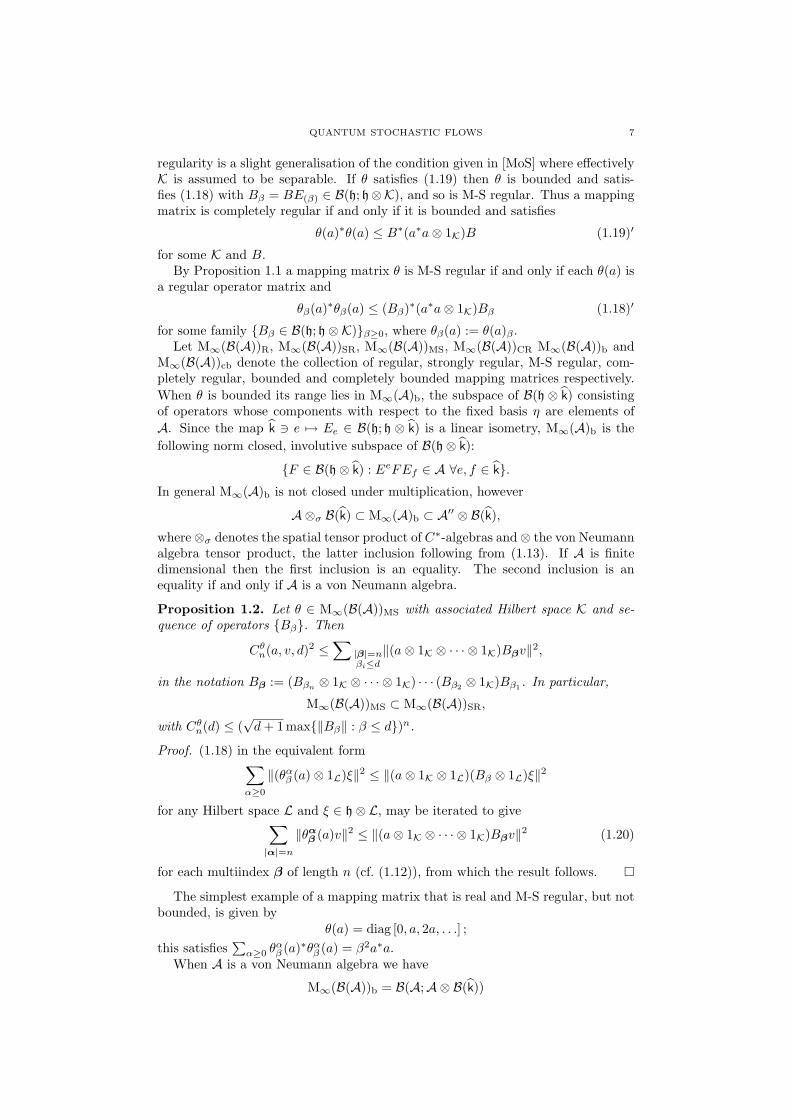
regularity is a slight generalisation of the condition given in [MoS] where effectivelyK is assumed to be separable. If θ satisfies (1.19) then θ is bounded and satis-fies (1.18) with Bβ = BE(β) ∈ B(h; h⊗K), and so is M-S regular. Thus a mappingmatrix is completely regular if and only if it is bounded and satisfies

θ(a)∗θ(a) ≤ B∗(a∗a⊗ 1K)B (1.19)′

for some K and B.By Proposition 1.1 a mapping matrix θ is M-S regular if and only if each θ(a) is

a regular operator matrix and

θβ(a)∗θβ(a) ≤ (Bβ)∗(a∗a⊗ 1K)Bβ (1.18)′

for some family {Bβ ∈ B(h; h⊗K)}β≥0, where θβ(a) := θ(a)β .Let M∞(B(A))R, M∞(B(A))SR, M∞(B(A))MS, M∞(B(A))CR M∞(B(A))b and

M∞(B(A))cb denote the collection of regular, strongly regular, M-S regular, com-pletely regular, bounded and completely bounded mapping matrices respectively.When θ is bounded its range lies in M∞(A)b, the subspace of B(h ⊗ k) consistingof operators whose components with respect to the fixed basis η are elements ofA. Since the map k 3 e 7→ Ee ∈ B(h; h ⊗ k) is a linear isometry, M∞(A)b is thefollowing norm closed, involutive subspace of B(h⊗ k):

{F ∈ B(h⊗ k) : EeFEf ∈ A ∀e, f ∈ k}.In general M∞(A)b is not closed under multiplication, however

A⊗σ B(k) ⊂ M∞(A)b ⊂ A′′ ⊗ B(k),

where⊗σ denotes the spatial tensor product of C∗-algebras and⊗ the von Neumannalgebra tensor product, the latter inclusion following from (1.13). If A is finitedimensional then the first inclusion is an equality. The second inclusion is anequality if and only if A is a von Neumann algebra.

Proposition 1.2. Let θ ∈ M∞(B(A))MS with associated Hilbert space K and se-quence of operators {Bβ}. Then

Cθn(a, v, d)2 ≤

∑|β|=nβi≤d

‖(a⊗ 1K ⊗ · · · ⊗ 1K)Bβv‖2,

in the notation Bβ := (Bβn ⊗ 1K ⊗ · · · ⊗ 1K) · · · (Bβ2 ⊗ 1K)Bβ1 . In particular,

M∞(B(A))MS ⊂ M∞(B(A))SR,

with Cθn(d) ≤ (√d+ 1 max{‖Bβ‖ : β ≤ d})n.

Proof. (1.18) in the equivalent form∑α≥0

‖(θαβ (a)⊗ 1L)ξ‖2 ≤ ‖(a⊗ 1K ⊗ 1L)(Bβ ⊗ 1L)ξ‖2

for any Hilbert space L and ξ ∈ h⊗ L, may be iterated to give∑|α|=n

‖θαβ (a)v‖2 ≤ ‖(a⊗ 1K ⊗ · · · ⊗ 1K)Bβv‖2 (1.20)

for each multiindex β of length n (cf. (1.12)), from which the result follows. �

The simplest example of a mapping matrix that is real and M-S regular, but notbounded, is given by

θ(a) = diag [0, a, 2a, . . .] ;this satisfies

∑α≥0 θ

αβ (a)∗θαβ (a) = β2a∗a.

When A is a von Neumann algebra we have

M∞(B(A))b = B(A;A⊗ B(k))


and, for completely bounded mapping matrices, the next result shows that

θ is normal ⇔ θ ∈ M∞(B(A))CR ⇔ θ ∈ M∞(B(A))MS.

Proposition 1.3. Let A be a von Neumann algebra, and let θ ∈ M∞(B(A)).(a) If θ is M-S regular then each θαβ is ultraweakly continuous.(b) If θ is completely bounded and ultraweakly continuous then θ is completely

regular.(c) Let θ be bounded. Then θ is ultraweakly continuous if and only if each θαβ

is.(d) Let θ be bounded and completely positive. If θββ is ultraweakly continuous

then θαβ is ultraweakly continuous for each α.

Proof. The proof of parts (a), (c) and (d) uses the facts that the weak and ultraweaktopologies coincide on bounded sets, and that a bounded operator between vonNeumann algebras is ultraweakly continuous if it preserves the limit of all boundedincreasing nets of positive elements ([Tak], Corollary III.3.11). So let (aλ) be abounded increasing net in A+ with least upper bound a.

(a) In this case ‖θαβ (aλ)‖ ≤ ‖θαβ‖‖a‖, so it suffices to show that θαβ (aλ − a) → 0weakly. Let {Bβ} be the operators associated with θ as in (1.18), then aλ ⊗ 1K →a⊗ 1K strongly, so

‖θαβ (aλ − a)v‖2 ≤ ‖[(aλ − a)⊗ 1K]Bβv‖2 → 0, v ∈ h.

Thus θαβ (aλ) → θαβ (a) strongly, and so also weakly.(b) By Haagerup’s version of the Wittstock-Paulsen Theorem for normal com-

pletely bounded maps ([Haa]), θ(a) = V ∗(a⊗ 1L)W for some Hilbert space L andoperators V,W ∈ B(h ⊗ k; h ⊗ L). Therefore θ satisfies (1.19)′ with B = ‖V ‖W ,and so is completely regular.

(c) Let θ be bounded. Suppose first that each θαβ is ultraweakly continuous. Since‖θ(aλ)‖ ≤ ‖θ‖‖a‖, it suffices to show that 〈(uγ), θ(aλ − a)(vγ)〉 → 0 for (uγ), (vγ)from the dense subspace h00 of ⊕γ≥0h defined in (1.5). But this follows immediatelyfrom the ultraweak and therefore weak convergence θαβ (aλ) → θαβ (a), for each α, β.Conversely, if θ is ultraweakly continuous then, by (1.8), each θαβ is a compositionof ultraweakly continuous maps, and so is ultraweakly continuous.

(d) This follows from the fact that if θ is bounded and CP then∑α≥0

‖θαβ (a)u‖2 =‖S∗π(a)SE(β)u‖2

≤‖S‖2‖π(a)SE(β)u‖2 = ‖S‖2〈u, θββ(a∗a)u〉,

where S∗π(·)S is a Stinespring decomposition of θ ([Sti],[Tak]). �

Corollary 1.4. Let A be finite dimensional, then

M∞(B(A))cb = M∞(B(A))b = M∞(B(A))CR.

Proof. The first equality follows from the fact that bounded linear maps betweenC∗-algebras are completely bounded when the source space is finite dimensional([HuT],[Smi]). Since all vector space topologies on a finite dimensional space coin-cide, A is a von Neumann algebra and each θαβ is ultraweakly continuous. Thereforethe second equality follows from parts (b) and (c) of the proposition. �

2. Quantum Stochastic Processes

In this section we describe the approach to quantum stochastic calculus (QSC)with infinite degrees of freedom developed by Mohari and Sinha ([MoS],[Moh],[Par]).


Our account allows sufficient flexibility to go beyond the context of unital ∗-homo-morphic flows treated by them. Let H = h ⊗ F , the Hilbert space tensor productof the initial space and the symmetric Fock space over L2(R+; k). For each testfunction f ∈ L2(R+; k), define the sequence, {fα}α≥0, of complex-valued functionson R+ using the orthonormal basis η:

f0(t) = 1; f i(t) = 〈ei, f(t)〉, i ≥ 1.

Thus f i ∈ L2(R+) for each i ≥ 1.We ensure that most of the apparently infinite sums that appear in what follows

have only finitely many nonzero terms by working with test functions from thefollowing dense subspace:

M = M[η] := {f ∈ (L2 ∩ L∞loc)(R+; k) : f i 6= 0 for only finitely many i}.

For f ∈ M, definedim f := max{α ≥ 0 : fα 6= 0}. (2.1)

Processes on a Hilbert Space. A subset S of M is admissible if

f ∈ S ⇒ f[0,t] ∈ S ∀t ≥ 0;

ES := Lin{ε(f) : f ∈ S} is dense in F .

Here ε(f) := ((n!)− 12 f⊗n) is the exponential vector for the test function f and

f[0,t] := f1[0,t] where 1[0,t] is the indicator function of the time interval [0, t]. Anadmissible subset S of M is fully admissible if

S [N ] := {(f1, . . . , fN ) : f ∈ S,dim f ≤ N} (2.2)

is an admissible subset of L2(R+; CN ) for each N ≥ 1. Full admissibility is a usefulconcept for reducing proofs to the case of finite dimensional noise. Clearly M isfully admissible itself; another fully admissible set of particular use for us is

S = S[η] := Lin{ek1J : k ∈ N, J ⊂ R+ a bounded interval}.

Whenever we work with a particular representative of an element of S, for examplefor the semigroup representation of solutions of QSDE’s proved in Theorem 3.1, wewill choose the right continuous version.

Operator adaptedness is defined using the increasing time indexed family ofsubspaces Ht := h ⊗ Ft of H, where Ft ⊂ F is the symmetric Fock space overL2([0, t]; k) ⊂ L2(R+; k). For an admissible set S, an ES-process on h is a familyX =(Xt)t≥0 of operators on H each having domain h� ES , which is weakly measurableand adapted :

(i) ∀ζ ∈ H the map t 7→ 〈ζ,Xtuε(f)〉 is measurable;(ii) Xtuε(f[0,t]) ∈ Ht, and Xtuε(f) = (Xtuε(f[0,t]))⊗ ε(f[t,∞[);

for all u ∈ h and f ∈ S. Since pointwise limits of measurable functions are measur-able, it suffices for (i) to hold for all ζ in some dense subset of H, such as h � ES′for an admissible set S ′. An ES -process X and ES′ -process Y are called adjointprocesses if

X∗t ⊃ Yt for a.a. t.

Thus an ES -process X has an ES′ -adjoint if DomX∗t ⊃ h � ES′ for all t; the ES′ -

adjoint process X∗· |h�ES′ is denoted X†. Two ES -processes X and X ′ are indistin-

guishable if

∀ζ ∈ H, ξ ∈ h� ES 〈ζ, (Xt −X ′t)ξ〉 = 0 for a.a. t.

Clearly H may be replaced by any dense subset such as h � ES′ for an admissibleset S ′. Indistinguishable processes are identified, and the resulting linear space is


denoted P(h, ES). The subspace of ES -processes having an ES′ -adjoint is denotedP‡(h, E(S′,S)); the map † is conjugate linear and involutive in the obvious sense:

X ∈ P‡(h, E(S′,S)) ⇒ X† ∈ P‡(h, E(S,S′)), and (X†)† = X. (2.3)

For discussing products of processes and quantum stochastic integrals, strongerproperties are needed. An ES -process X is measurable (respectively continuous) ifit satisfies

t 7→ Xtξ is strongly measurable (resp. continuous), (2.4)By Pettis’ Theorem X ∈ P(h, ES) is measurable if and only if each X·ξ is Lebesgue-essentially separably-valued. For measurable ES -processes X and X ′, indistin-guishability is equivalent to

∀ξ ∈ h� ES Xtξ = X ′tξ for a.a. t.

An ES -process X on h is a bounded, contraction, isometry, coisometry or unitaryprocess if (for some version ofX) each operatorXt has that property. For a boundedprocess X the weak adaptedness condition amounts to (the continuous extensionof) Xt belonging to B(Ht).

An ES -process X on h is E(S′,S)-regular if, for all f ∈ S ′, g ∈ S and T > 0,

sup{|〈uε(f), Xtvε(g)〉| : ‖u‖ = ‖v‖ = 1, t ∈ [0, T ]} <∞; (2.5)

it is ES-regular if, for all g ∈ S and T > 0,

sup{‖Xtvε(g)‖ : ‖v‖ = 1, t ∈ [0, T ]} <∞. (2.6)

An element L of M∞(P(h, ES)) is called an ES-process matrix ; when L is inM∞(P‡(h, E(S′,S))) its adjoint L† ∈ M∞(P‡(h, E(S,S′))) is defined by

(L†)αβ = (Lβα)†.

Stochastic Integration. The integrator processes of the theory, [Λαβ ]∞α,β=0, aredefined in terms of the orthonormal basis η by

Creation: Λ0j (t) := a∗(ej1[0,t]);

Conservation: Λij(t) := dΓ(|ej〉〈ei| ⊗M[0,t]);Annihilation: Λi0(t) := a(ei1[0,t]);Time: Λ0

0(t) := t1;

where a∗, dΓ and a denote, respectively, Fock space creation, differential secondquantisation and annihilation, M[0,t] is the operator of multiplication by 1[0,t] onL2(R+), |ej〉〈ei| is the Dirac dyad acting on k by ζ 7→ 〈ei, ζ〉ej , and L2(R+; k)is identified with the Hilbert space tensor product k ⊗ L2(R+) (see [HuP],[Mey],[Par]).

An ES -process X is stochastically integrable if it satisfies

t 7→ Xtξ is locally square integrable .

In particular X is measurable. Let PSI(h, ES) denote the collection of stochasticallyintegrable ES -processes. For each pair of indices α, β the QS integral

∫ t0Xs dΛαβ(s) is

defined by Hudson and Parthasarathy, and shown to form a continuous ES -process(∫ t0Xs dΛαβ(s))t≥0, when X is stochastically integrable ([HuP]). An alternative

approach to the delicate question of the existence of such QS integrals on theexponential domain is given in [Bia]. Let L be an ES -process matrix such that eachcomponent process Lαβ is stochastically integrable, thus L ∈ M∞(PSI(h, ES)). Then,for each N ≥ 0, we may form the ES -process Λ[N](L) given by

Λ[N](L)t =∑

α,β≤N

∫ t

0

Lαβ(s) dΛβα(s).


The process matrix L is stochastically integrable if∫ t

0

∑α≥0

‖Lαβ(s)uε(f)‖2 ds <∞ (2.7)

for all choices of u ∈ h, f ∈ S, t ≥ 0 and β ≤ dim f . The collection of stochasticallyintegrable ES -process matrices is denoted M∞(P(h, ES))SI.

Theorem 2.1 ([Moh],[MoS],[Par]). Let S be an admissible subset of M and letL ∈ M∞(P(h, ES))SI. Then there is an ES-process denoted Λ(L) satisfying

(i) limN→∞

sup0≤t≤T

‖[Λ(L)t − Λ[N](L)t]uε(f)‖ = 0;

(ii) ‖Λ(L)tuε(f)‖2 ≤ 2eνf (t)

dim f∑β=0

∫ t

0

∑α≥0

‖Lαβ(s)uε(f)‖2 dνf (s);

for all u ∈ h, f ∈ S and t, T ≥ 0, where dνf (s) = (1 + ‖f(s)‖2) ds, and dim f isdefined in (2.1).

Notice that the estimate (ii) implies that the process Λ(L) is continuous. Thefirst fundamental formula of QSC reads

〈uε(f),Λ(L)tvε(f)〉 =∫ t

0

fα(s)gβ(s)〈uε(f), Lαβ(s)vε(g)〉 ds, (2.8)

with the summation convention operating, and fα(s) := fα(s), for f ∈ M, g ∈S, u, v ∈ h and t ≥ 0. Here the sum is finite since f, g ∈ M. If M is a stochasticallyintegrable family of ES′ -processes for another admissible set S ′, then

〈Λ(L)tuε(f),Λ(M)tvε(g)〉 =∫ t

0

fα(s)gβ(s){〈Λ(L)suε(f),Mα

β (s)vε(g)〉

+ 〈Lβα(s)uε(f),Λ(M)svε(g)〉+ 〈Liα(s)uε(f),M iβ(s)vε(g)〉

}ds (2.9)

for u, v ∈ h, f ∈ S, g ∈ S ′ and t ≥ 0, with summation over α, β and i. Herethe sum over i is an infinite one — that it converges to an integrable functionof s is ensured by the stochastic integrability of L and M . This is the secondfundamental formula of QSC and is a rigorous formulation of the quantum Itoformula. Thus QS integration may be viewed as a map Λ : M∞(P(h, ES))SI →P(h, ES); its image consists of continuous processes. We mention one importantconsequence of the first fundamental formula: for L ∈ M∞(P‡(h, E(S′,S))), if L andL† are both stochastically integrable then Λ(L) ∈ P‡(h, E(S′,S)) and Λ(L†) = Λ(L)†.

Independence of Integrators. The assumption of full admissibility (2.2) reducesthe problem of independence of QS integrators to the case of finite dimensionalquantum noise.

Proposition 2.2. Let S and S ′ be fully admissible subsets of M, and suppose thatL ∈ M∞(P‡(h, E(S′,S))) with each Lαβ and Lα†β stochastically integrable.

(a) If, for each ξ ∈ h�ES , ζ ∈ h�ES′ and t ≥ 0, the sequence (〈ζ,Λ[N](L)tξ〉)∞N=0

is eventually zero then L = 0.(b) If L ∈ M∞(P(h, ES))SI and Λ(L) = 0 then L = 0.

Proof. (a) For each N ≥ 1 let JN be the isometry h⊗Γ(L2(R+; CN )) → H definedby continuous linear extension of the prescription

JN : uε(f) 7→ uε(∑Ni=1f

iei) (2.10)

Fix N ≥ 1. The hypothesis and (2.8) imply that

〈uε(f),Λ[N](L)tvε(g)〉 = 0


for all t ≥ 0, u, v ∈ h and f ∈ S ′, g ∈ S with dim f,dim g ≤ N . Now the matrix{J∗NLαβJN}Nα,β=0 is a collection of (N + 1)2 ES[N] -processes, with ES′[N]-adjoints{J∗NLαβ

†JN}, and by the above they satisfy∫ t

0

J∗NLαβ(s)JN dΛβα(s) = 0,

(with sums only up to N) as a QS integral on h ⊗ Γ(L2(R+; CN )). The finitedimensional result ([L], Theorem 5.1) implies that J∗NL

αβJN = 0 for all α, β ≤ N ,

and the result follows since ‖ξ‖ = limN→∞ ‖J∗Nξ‖ for all ξ ∈ H.(b) If L ∈ M∞(P(h, ES))SI then Λ(L) exists as an ES -operator process by The-

orem 2.1. If Λ(L) = 0 then since S ⊂ M, each sequence (〈ξ,Λ[N](L)tξ〉)∞N=0 iseventually zero and so (a) applies. �

Remark. The fact that L itself need not be assumed to be stochastically integrablecan be useful.

Processes on a C∗-algebra. For an admissible set S, an ES-process on A, theinitial algebra fixed at the beginning of Section 1, is a map k : A → P(h, ES) suchthat each kt(a) is affiliated to the von Neumann algebra A′′ ⊗ B(F), that is

kt(a)(a′ ⊗ 1F )ξ = (a′ ⊗ 1F )kt(a)ξ ∀a′ ∈ A′, ξ ∈ h� ES . (2.11)

The linear space of ES -processes on A is denoted P(A, ES). An ES -process k on Ais continuous if each ES -process k·(a) on h is (see (2.4)); it is linear if each kt is; itis unital if each kt(1) equals 1|h�ES ; it is a bounded process if each operator kt(a)is bounded and each kt, viewed as a map A → B(H), is a bounded linear operator;and is a contraction process if furthermore each kt is a contraction. Thus boundedES -processes on A satisfy

kt(A) ⊂ A′′ ⊗ B(F).

An ES -process k on A is E(S′,S)-regular if

sup{|〈uε(f), [kt(a1)− kt(a2)]vε(g)〉|

‖u‖‖a1 − a2‖‖v‖: t ∈ [0, T ], u, v, a1 − a2 6= 0

}<∞, (2.12)

and ES-regular if

sup{‖[kt(a1)− kt(a2)]vε(g)‖

‖a1 − a2‖‖v‖: t ∈ [0, T ], v, a1 − a2 6= 0

}<∞, (2.13)

for all T > 0, f ∈ S ′ and g ∈ S. Thus contraction ES -processes are ES -regular.Regularity properties of processes are key to the uniqueness of QSDE solutions;they are closely related to the regularity of QSDE coefficients; and they play animportant role in the algebraic characterisation of QSDE solutions ([LW2]).

A linear ES -process on A is completely positive if∑p,q〈ξp, kt(a∗paq)ξq〉 ≥ 0

for all t ≥ 0 and each finite collection {(ap, ξp)} from A × (h � ES), and it is∗-homomorphic if it satisfies

〈ξ, kt(a∗a)ξ〉 = ‖kt(a)ξ‖2,

in other words kt(a∗a) = kt(a)∗kt(a).If k ∈ P(A, ES) and each k·(a) ∈ P‡(h, E(S′,S)) then, following (2.3),

k†t (a) := kt(a∗)†

defines an adjoint ES′ -process k† to k; the collection of such processes is denotedP‡(A, E(S′,S)). Processes in P‡(A, E(S,S)) satisfying k† = k are called real. Note


the obvious symmetry in the above definitions: for k ∈ P‡(A, E(S′,S)), k is E(S′,S)-regular if and only if k† is E(S,S′)-regular. A process k ∈ P‡(A, E(S′,S)) is weaklymultiplicative if it satisfies

〈k†t (a∗)ξ, kt(b)ζ〉 = 〈ξ, kt(ab)ζ〉,

in other words kt(ab) = k†t (a∗)∗kt(b). Thus k ∈ P(A, ES) is ∗-homomorphic if andonly if it is linear, real and weakly multiplicative.

The following relationships mirror familiar C∗-algebraic facts ([LP2], Proposi-tion 2.1).

Lemma 2.3. Let k be an ES-process on A. If k is ∗-homomorphic then k is a CPcontraction process with k·(1) orthogonal projection valued. If k is CP then k isreal, and is a contraction process if and only if k·(1) is a contraction process on h.

When A is a von Neumann algebra, a bounded process k on A is normal if eachmap kt is normal.

Terminology refinement. In [LP2] what we here call an ES -process on A wascalled an ES -flow, and P(A, ES) there denoted the collection of linear maps A →P(h, ES), without the restriction of affiliation imposed here (2.11). Here we reservethe term flow for E(S′,S)-regular ES -processes on A weakly satisfying a QSDE of theform (0.1). Theorem 3.1 below shows that flows (in the present sense) are uniquelydetermined by the coefficients of the QSDE, and that they are automatically linearand satisfy the affiliation condition.

3. Quantum Stochastic Differential Equations

In this section we analyse the linear quantum stochastic differential equation

dkt = kt ◦ θαβ dΛβα(t), k0(a) = a⊗ 1, (3.1)

governed by a mapping matrix θ, for ES -flows on the C∗-algebra A. In the workof Mohari and Sinha various relations were imposed on the mapping matrix θ inorder to ensure that the solution to the QSDE enjoyed certain algebraic properties.However at this stage we impose only minimal conditions on θ in order to studythe equation in a more general setting, before deriving the necessary and sufficientstructure equations for complete positivity of the flow in the next section. Inparticular we discuss the notion of weak and strong solutions, giving conditionsthat ensure the existence of solutions, and we prove that weak solutions, subjectto the very mild condition of weak regularity, are unique and satisfy a semigrouprepresentation property, as in the case of finite dimensions of quantum noise.

Weak and Strong Solutions. Let S and S ′ be admissible sets. An E(S′,S)-weaksolution of (3.1) is an ES -process k on A that satisfies

s 7→ fα(s)gβ(s)〈uε(f), ks(θαβ (a))vε(g)〉 is locally integrable, (3.2a)

and〈uε(f), kt(a)vε(g)〉 =〈uε(f), avε(g)〉

+∫ t

0

fα(s)gβ(s)〈uε(f), ks(θαβ (a))vε(g)〉 ds(3.2b)

for all u, v ∈ h, f ∈ S ′, g ∈ S, a ∈ A and t ≥ 0. An ES-strong solution of (3.1) is anES -process k such that

[k·(θαβ (a))] ∈ M∞(P(h, ES))SI ∀a ∈ A, (3.3a)


(see (2.7)) and the corresponding integral equation holds:

kt(a) = a⊗ 1 +∫ t

0

ks(θαβ (a)) dΛβα(s). (3.3b)

By the first fundamental formula, k ∈ P(A, ES) is an ES -strong solution if andonly if k satisfies (3.3a) and is an E(S′,S)-weak solution for any/every admissible setS ′; by the second fundamental formula ES -strong solutions are continuous.

We shall make use of the following notation: given φ ∈ M∞(B(A)) and w, z ∈c00(N), define a bounded linear map φw,z on A by

φw,z(a) = wαφαβ(a)zβ , (3.4)

where wα := wα and we set w0 = z0 = 1. Thus if k ∈ P(A, ES) is a linear processsatisfying (3.2a) then k is an E(S′,S)-weak solution of (3.1) if and only if it satisfies

〈uε(f), kt(a)vε(g)〉 = 〈uε(f), avε(g)〉+∫ t

0

〈uε(f), ks(θf(s),g(s)(a))vε(g)〉 ds,

where f(s) = {f i(s)} ∈ c00(N) and similarly for g(s), for representatives from themeasure equivalence classes of f and g.

Uniqueness of Solutions and the Semigroup Representation. A conse-quence of working with test functions from the set M is that results in the finitedimensional noise setting whose proofs rely only on manipulations of matrix ele-ments of the form 〈uε(f), kt(a)vε(g)〉 often carry over to the infinite dimensionalsetting, since only a finite (but arbitrarily large) number of components of the testfunctions f and g are nonzero. In particular the uniqueness result and semigrouprepresentation of weak solutions given in Theorem 3.1 of [LP2] both remain validwith a very similar proof.

Theorem 3.1. Let S and S ′ be admissible sets.(ai) For θ ∈ M∞(B(A)), the QSDE (3.1) has at most one E(S′,S)-regular E(S′,S)-

weak solution k. If such a k exists then it is linear.(aii) For k ∈ P(A, ES), if S ∩ S ′ ⊃ S then k is an E(S′,S)-weak solution of (3.1)

for at most one mapping matrix θ.(b) For θ ∈ M∞(B(A)) and k ∈ P(A, ES), if S ∪ S ′ ⊂ S then the following are

equivalent:(i) k is an E(S′,S)-regular E(S′,S)-weak solution of (3.1).(ii) For f ∈ S ′ and g ∈ S, with discontinuities contained in the set {0 =

t0 < t1 < · · · < tn < tn+1 = ∞},

〈uε(f), kt(a)vε(g)〉 = 〈u,P [0]t1−t0 ◦ · · · ◦ P

[i]t−ti(a)v〉〈ε(f), ε(g)〉 (3.5)

for t ∈ [ti, ti+1[ where, in the notation (3.4), P [k] is the one-parametersemigroup on A with generator θw,z where w = f(tk) and z = g(tk).

Proof. (ai) Let 1k and 2k be E(S′,S)-regular E(S′,S)-weak solutions of (3.1). Appli-cation of (3.2b) to 〈uε(f), [ 1kt(a)− 2kt(a)]vε(g)〉 may be iterated; E(S′,S)-regularityapplied after n iterations yields a bound of the form (n!)−1C1C

n2 as in [LP2] —

the only difference being that here the constants depend on the dimensions of thetest functions. The necessary linearity then follows from the same argument byapplying (3.2b) to 〈uε(f), [kt(a+ λb)− kt(a)− λkt(b)]vε(g)〉 and iterating.

(aii) Suppose that k is an E(S′,S)-weak solution of (3.1) for mapping matrices 1θ

and 2θ. Since k satisfies (3.2b) for both matrices

0 =∫ t

0

fα(s)gβ(s)〈uε(f), [ks(1θαβ (a))− ks(2θαβ (a))]vε(g)〉 ds.


Putting f = w1[0,1] and g = z1[0,1], where w, z ∈ c00(N), continuity of the integrandon [0, 1] means that it vanishes identically on that interval. Considering the valueat 0, we obtain the identity

wα[1θαβ (a)− 2θαβ (a)]zβ = 0;

varying w and z gives 1θ(a) = 2θ(a) as required.(bi ⇒ bii) This is proved exactly as in the finite dimensional case ([LP2]).(bii ⇒ bi) This follows easily from the Fundamental Theorem of Calculus. �

Remarks. (i) It is clear from the semigroup representation (3.5) that any E(S′,S)-regular E(S′,S)-weak solution k to the QSDE (3.1) satisfies the affiliation condi-tion (2.11).

(ii) If the coefficient matrix θ is a function of time, with sufficiently regulardependence, then the semigroups in the representation (3.5) should be replaced byevolution operators governed by equations of the form

dPt = Pt ◦ θw,z(t, ·) dt, P0 = idA.

Flows and Generators. The previous theorem allows us to establish the followingterminology: when (3.1) has an E(S′,S)-regular E(S′,S)-weak solution k, we call θ theQS generator of k, and k the E(S′,S)-flow weakly generated by θ.

Our next result shows that reality passes from generator to flow and vice versa.

Proposition 3.2. Suppose that θ ∈ M∞(B(A)) weakly generates an E(S′,S)-flow k,for some admissible sets S and S ′. Then the following hold.

(a) The following are equivalent:(i) k ∈ P‡(A, E(S′,S)).(ii) θ† weakly generates an E(S,S′)-flow j.In this case j = k†.

(b) If S = S ′ ⊃ S then the following are equivalent:(i) k is real.(ii) θ is real.

(c) If A is a von Neumann algebra and k is bounded, then the following areequivalent:(i) k is normal.(ii) each θαβ is ultraweakly continuous.

Proof. (ai ⇒ aii) This is an immediate consequence of (3.2b) applied to

〈kt(a∗)uε(f), vε(g)〉 − 〈uε(f), avε(g)〉.

(aii ⇒ ai) This yields to the argument used in the proof of Theorem 3.1(ai),since application of (3.2b) to the difference

〈jt(a∗)uε(f), vε(g)〉 − 〈uε(f), kt(a)vε(g)〉,

may be iterated.(b) This follows from (a) and Theorem 3.1(aii).(c) Since the set of ultraweakly continuous maps in B(A) is norm closed, the

equivalence follows easily from the semigroup representation (3.5) and the fact thatthe ultraweak and weak topologies coincide on bounded sets. �

Remark. The implications (ai ⇒ aii) and (bi ⇒ bii) are valid without weak regu-larity — the existence of a weak solution suffices.


Existence of Solutions. If θ ∈ M∞(B(A)) has only finitely many nonzero com-ponents then it is a straightforward matter to generate the unique, EM-regular,EM-strong solution to the equation (3.1) using a Picard iteration method (see, forexample, [Eva] or [HLP]). However the estimates involved in the construction ofthese solutions depend on the number of nonzero components, and so more sophis-ticated methods are required in the general case. The first existence theorem for(3.1) with an infinite number of nonzero coefficients was obtained by Mohari andSinha ([MoS]). We give a refinement, with a simplified proof, as described in [Mey].

Recall the weak and strong regularity conditions (2.12) and (2.13) for processeson the algebra A.

Theorem 3.3. Let θ ∈ M∞(B(A))R. Then (3.1) has an EM-strong solution k whichis E(M,M)-regular. Moreover, if θ ∈ M∞(B(A))SR then the process k is EM-regular.

Proof. Consider the Picard iteration scheme

k{0}t (a) = a⊗ 1; k

{n+1}t (a) = a⊗ 1 +

∫ t

0

k{n}s (θαβ (a)) dΛβα(s).

Using the relationship∑α≥0

∑β≤d

Cθn(θαβ (a), u, d)2 = Cθn+1(a, u, d)

2, (3.6)

an inductive argument shows that [k{n}· (θαβ (a))] is stochastically integrable, so thatthe scheme is well-defined, and for f ∈ M and t ∈ [0, T ],

‖[k{n}t (a)− k{n−1}t (a)]uε(f)‖2 ≤ (n!)−1C(f, t)nCθn(a, u, d)

2‖ε(f)‖2

where C(f, t) = 2νf (t) exp νf (t) and d = dim f . This implies the estimate

‖k{n}t (a)uε(f)‖ ≤n∑p=0

(p!)−1/2C(f, T )p/2Cθp(a, u, d)‖ε(f)‖. (3.7)

It follows that kt(a)uε(f) = limn k{n}t (a)uε(f) exists and defines an adapted mea-

surable process k satisfying

‖kt(a)uε(f)‖ ≤∑n≥0

(n!)−1/2C(f, T )n/2Cθn(a, u, d)‖ε(f)‖. (3.8)

Introducing a factor of 2−n/2× 2n/2 into the summand above, the Cauchy-Schwarzinequality and (3.6) then gives∑α≥0

∑β≤d

‖kt(θαβ (a))uε(f)‖2 ≤∑n≥0

(n!)−1C(f, T )n2n+1Cθn+1(a, u, d)2‖ε(f)‖2, (3.9)

and the right hand side converges since θ is regular. Thus [k·(θαβ (a))] is stochasti-cally integrable, and the estimate

‖[kt(a)− k{n}t (a)]uε(f)‖ ≤

∑p≥n+1

(p!)−1/2C(f, T )p/2Cθp(a, u, d)‖ε(f)‖

now allows us to deduce that k satisfies the integral equation (3.3b).Examination of the iteration scheme that generates k reveals the identity:

〈uε(f), kt(a)vε(g)〉 =

〈ε(f), ε(g)〉∑n≥0

∑|α|=|β|=n0≤αi,βi≤d′

〈u, θαβ (a)v〉

∫ t

0

dtn · · ·∫ t2

0

dt1 hβα(t) (3.10)


where d′ = max{dim f,dim g}, hβα(t) =

∏ni=1 h

βiαi

(ti) and hβiαi

= fαigβi . It follows

that

|〈uε(f), kt(a)vε(g)〉| ≤ |〈ε(f), ε(g)〉|‖u‖‖a‖‖v‖∑n≥0

(n!)−1

(∫ t

0

p(s)ds)n

(3.11)

where p(s) =∑α,β≥0 ‖hβα(s)θαβ‖, thus k is E(M,M)-weakly regular. Note that if

θ ∈ M∞(B(A))SR then EM-strong regularity follows from (3.8). �

The solution constructed in Theorem 3.3 will be denoted kθ. Propositions 1.2and 1.3, and Corollary 1.4 thus give useful sufficient conditions for the existence ofa strong solution of (3.1).

The following property is used in the discussion of ∗-homomorphic processes inSection 6. An ES -process k on A is sequentially strongly continuous if it satisfies

a, a1, a2, . . . ∈ A, an → a strongly =⇒ kt(an)ξ → kt(a)ξ ∀ξ, t.

Sequential weak continuity is defined analogously.

Proposition 3.4. Let θ ∈ M∞(B(A))MS. Then kθ and each of its Picard approxi-mants k{n} are sequentially strongly continuous.

Proof. Let f ∈ M, a, a1, a2, . . . ∈ A with ai → a strongly, and put M = supi ‖ai‖and d = dim f . In the notation (1.17), the iterated form of M-S regularity (1.20)implies that Cθn(ai − a, u, d) → 0 for each n, and strong regularity implies thatCθn(ai−a, u, d) ≤ 2M‖u‖Cθn(d). Thus the sequential strong continuity of each k{n}

follows from (3.7). The estimate (3.8) now gives ‖kθt (ai − a)uε(f)‖ → 0 by theDominated Convergence Theorem for series. �

Continuous Dependence on Test Functions. We conclude this section witha continuity result for the solution to (3.1) when θ is a regular mapping matrix.From Theorem 3.3 we see that the map (u, a, v) 7→ 〈uε(f), kt(a)vε(g)〉 is continuousfor fixed f and g if θ is regular. Now we show that, if u, a and v are fixed, thereis a continuous dependence on the test functions within certain restrictions on thenumber of nonzero components.

Proposition 3.5. Let θ ∈ M∞(B(A))R. For f, g ∈ M and T > 0, if {fn} and {gn}are sequences in M satisfying

(i) limn→∞ ‖fn − f‖L2 = limn→∞ ‖gn − g‖L2 = 0,(ii) supn{max(dim fn,dim gn)} <∞,

thenlimn→∞

supt∈[0,T ]

|〈uε(fn), kθt (a)vε(gn)〉 − 〈uε(f), kθt (a)vε(g)〉| = 0

for all u, v ∈ h and a ∈ A.

Proof. Letting d′ equal the maximum dimension of all of the test functions involved,the result follows from the representation (3.10) as in Proposition 3.5 of [LP2]. �

4. Completely Positive Flows

In this section we assume that θ weakly generates an E(S,S)-flow, for some suffi-ciently large admissible set S. Under this assumption we establish necessary andsufficient conditions on θ for the flow to be completely positive. This is the infinitedimensional extension of Theorem 4.1 in [LP2], where the boundedness of eachof the finite number of maps θαβ ensures that θ generates a flow. Here, with thisexistence assumption, we may exploit the results of [LP2].

Recall the definition of the transformed mapping matrices (1.16).


Theorem 4.1. Let θ ∈ M∞(B(A)) and suppose that θ weakly generates an E(S,S)-flow k, where S is a fully admissible set such that each S [N ] is dense in L2(R+; CN ).

(a) The following are equivalent:(i) k is completely positive.(ii) θ00 is real and there is a quadruple Q = (π,K, δ, {Wi}) consisting of

a representation (π,K) of A, a π-derivation δ : A → B(h;K) and asequence {Wi} in B(h;K) such that

∂θ00(a1, a2) = δ(a1)∗π(1)δ(a2)

θi0(a)−W ∗i π(1)δ(a) = θi0(1)a

θ0j (a)− δ†(a)π(1)Wj = aθ0j (1)

θij(a) + δija = W ∗i π(a)Wj .

(4.1)

(iii) There is a quadruple P = (π,K, {Kγ}, {Wγ}) consisting of a represen-tation (π,K) of A and sequences of operators {Kγ} in B(h) and {Wγ}in B(h;K) such that θ = ψ + φ, where

ψαβ (a) = W ∗απ(a)Wβ and φαβ(a) = δα0 aKβ + δ0βK

∗αa. (4.1)′

(bi) Q may be chosen so that

(π,K) is unital, (4.2)

and the following minimality condition is satisfied:

K = K0 where K0 = Lin{δ(a)u0 + π(a)Wiu

i : a ∈ A, (uγ) ∈ h00

}. (4.3)

(bii) P may be chosen so that (π,K) is unital, Kγ ∈ A′′ and

K = K0 where K0 = Lin{π(a)Wαu

α −W0au0 : a ∈ A, (uγ) ∈ h00

}. (4.3)′

(c) Quadruples Q satisfying (4.1), (4.2) and (4.3) are unique: if Q′ satisfies(4.1) then there is a unique isometry V : K → K′ such that

VWi = π′(1)W ′i ; V δ(a) = π′(1)δ′(a); V π(a) = π′(a)V. (4.4)

Moreover, V is an isomorphism if and only if Q′ also satisfies (4.2) and(4.3)

(d) Suppose that A is a von Neumann algebra and k is completely positive. Ifθαα is ultraweakly continuous, then so are θαβ and θβα for each β. If everyθαβ is ultraweakly continuous and Q is a quadruple satisfying (4.1) and theminimality condition (4.3), then π is normal.

Terminology. (i) The coboundary-like operator ∂ acts on linear maps ψ onthe algebra A to give sesquilinear maps ∂ψ : A × A → A in the followingmanner:

∂ψ(a1, a2) = ψ(a∗1a2)− a∗1ψ(a2)− ψ(a∗1)a2 + a∗1ψ(1)a2.

The map ∂ψ determines ψ up to the sum of a derivation and an anticom-mutator on A.

(ii) If (π,K) is a representation of the algebra A then a linear map δ : A →B(h;K) is a π-derivation if it satisfies the π-Leibnitz identity:

δ(a1a2) = δ(a1)a2 + π(a1)δ(a2).

It is well known that derivations A ⊂ B(h) → B(h) are bounded ([Rin]).An elementary argument with block matrices shows that π-derivations areautomatically bounded too.


Proof. First note that if (4.1) holds then, replacing K by π(1)K, δ by π(1)δ andWj by π(1)Wj , and restricting π to the Hilbert space π(1)K, it may be seen that(4.1) holds for a unital π. Similarly for (4.1)′.

Let θ[d] be the cut-off matrix (see (1.2)) viewed as an element of Md+1(B(A)),and let dk = kφ, the strong solution to the QSDE (3.1) on h ⊗ Γ(L2(R+; Cd)) forφ = θ[d], so that dk is an EM[d]-process ([LP2]). If Jd denotes the linear isometryh ⊗ Γ(L2(R+; Cd)) → H defined through (2.10), then by uniqueness of weaklyregular weak solutions ([LP2], Theorem 3.1(b)),

J∗dkt(a)Jd =dkt(a)|h�ES[d] , (4.5a)

and, for any ξ ∈ h� ES ,

〈ξ, kt(a)ξ〉 =〈J∗d ξ, dkt(a)J∗d ξ〉 (4.5b)

for all sufficiently large d. By continuity in test functions ([LP2], Proposition 3.5),it follows from (4.5) that k is completely positive if and only if each dk is com-pletely positive. Thus the implications (aii ⇒ ai, aiii ⇒ ai) follow from their finitedimensional counterparts ([LP2], Theorem 4.1).

(ai ⇒ aii, aiii), (b): Suppose that k is completely positive. Then, for each d, dkis completely positive and so Theorem 4.1 of [LP2] guarantees the existence of asequence of quadruples (dπ, dK, dδ, dW )d≥1 whose terms consist of a unital representa-tion (dπ, dK) ofA, a dπ-derivation dδ : A → B(h; dK) and an operator dW ∈ B(hd; dK),where hd = ⊕di=1h, such that

θ[d](a) =[

θ00(a) a dC∗ + dδ†(a) dWdCa+ dW ∗ dδ(a) dW ∗ dπ(a) dW

](4.6a)

where dC = [θ10(1) · · · θd0(1)]>, θ00 is real,

∂θ00(a, b) = dδ(a)∗ dδ(b) (4.6b)

and dK = dK0 wheredK0 = Lin{dδ(a)u0 + dπdW (b)u : a, b ∈ A, u0 ∈ h,u ∈ hd}.

For all e ≥ d let Ied ∈ B(hd; he) be the isometry u 7→ (u1, . . . , ud, 0, . . . , 0).It follows that (eπ, eK, eδ, eWIed) is a quadruple that satisfies (4.6), and so by theuniqueness part of Theorem 4.1 of [LP2] there is a (unique) isometry edU : dK → eKsuch that

edU dW = eWIed; edU dδ(a) = eδ(a); edU dπ(a) = eπ(a) edU.

The identity IfeIed = Ifd for all f ≥ e ≥ d leads to the consistency relationfeUedU = fdU , as can be seen by checking the actions on the dense set dK0, and thus({dK}, {edU}) is a directed system of Hilbert spaces ([KaR], p.886). Let (K, {dU})be its inductive limit. For 1 ≤ i ≤ d let Idi ∈ B(h; hd) denote the embedding of h

into the ith coordinate, that is Idi u = (0, . . . , 0, u, 0, . . . , 0). Since eU edU = dU forall e ≥ d the vector

dU dπ(a)[dδ(b)u+ dπ(c) dWIdi v], (4.7)

is independent of the choice of d (≥ i). It follows that

δ(a) := dUdδ(a) and Wi := dUdWIdi (d ≥ i),

define operators δ(a) and Wi in B(h;K) and since by construction K0 =⋃d≥1

dUdK0

is dense in K, and each dU is isometric, it also follows that each a ∈ A uniquelydetermines a bounded operator π(a) on K through the identities

π(a) dU = dU dπ(a).


The map a 7→ π(a) defines a unital representation (π,K) of A, the map a 7→ δ(a)defines a π-derivation, and the vector (4.7) equals

π(a)[δ(b)u+ π(c)Wiv].

The finite-dimensional structure (4.6) can now be rewritten in terms of thequadruple Q = (π,K, δ, {Wi}), which evidently satisfies (4.1), (4.2) and (4.3). Thus(aii) holds and (bi) is proved.

Finally, start with a quadruple Q satisfying (4.1–4). Since ∂θ00(A × A) ⊂ Ait follows from Theorem 2.1 of [ChE] that δ is implemented by an element W0

in the ultraweak closure of Lin{δ(a)b : a, b ∈ A}, that is δ(a) = π(a)W0 −W0a.Manipulating (4.1) gives

(δ(b1)c1)∗π(a)δ(b2)c2,W ∗i δ(b)c ∈ A ∀a, bk, ck ∈ A

and so W ∗0 π(a)W0,W

∗i W0 ∈ A′′. Define χ : A → A′′ by χ(a) = θ00(a)−W ∗

0 π(a)W0.Then ∂χ = 0, and so χ(a) = α(a) + (ac+ ca) for some real derivation α : A → A′′and c = c∗ ∈ A′′ ([LP2], Proposition 1.2). Applying Theorem 2.1 of [ChE] oncemore produces an h = h∗ ∈ A′′ such that α(a) = i(ha−ah). PuttingK0 = c−ih andKj = θ0j (1)−W ∗

0Wj gives a quadruple P = (π,K, {Kγ}, {Wγ}) that satisfies (4.1)′

and (4.3)′, with Kγ ∈ A′′. Thus (aiii) holds too, and (b) is proved.(c): Let Q = (π,K, δ, {Wi}) be any quadruple satisfying (4.1–4), and let Q′ be

a similar quadruple satisfying (4.1). The identity

〈π′(1)δ′(a)u0 + π′(b)W ′iui, π′(1)δ′(c)v0 + π′(d)W ′

jvj〉

=〈u0, ∂θ00(a, b)v0〉+ 〈ui, [θi0(b∗c)− θi0(b

∗)c]v0〉

+ 〈[θj0(d∗a)− θj0(d∗)a]u0, vj〉+ 〈ui, θij(b∗d)vj〉,

for (uγ), (vγ) ∈ h00, together with its unprimed version, and the totality condition(4.3), imply the existence of a unique linear isometry V : K → K′ satisfying

V {δ(a)u0 + π(b)Wjuj} = π′(1)δ′(a)u0 + π′(b)W ′

juj .

The identities (4.4) follow easily, moreover any other isometry V ′ ∈ B(K;K′) sat-isfying (4.4) agrees with V on the dense subspace K0, and so V = V ′. It is clearfrom the definition of V that it is unitary if Q′ also satisfies (4.3–4), and for theconverse note that the range of V lies in π′(1)K′.

(d): Suppose that A is a von Neumann algebra and k is completely positive. Ifθαα is ultraweakly continuous then, letting P be a quadruple as in (aiii), the estimate

|〈u,W ∗βπ(a)Wαv〉|2 ≤ ‖Wβu‖2〈v,W ∗

απ(a∗a)Wαv〉

shows that θβα is ultraweakly continuous moreover, by the reality of θ, θαβ is ultra-weakly continuous too. Now suppose that each θαβ is ultraweakly continuous andlet Q be a quadruple satisfying (4.1) and (4.3). To prove the normality of π itsuffices to check that 〈ξ, π(dλ)η〉 → 〈ξ, π(d)η〉 for any bounded increasing net (dλ)in A+ with least upper bound d, and for all vectors ξ, η ∈ K0. By sesquilinearitywe can write the inner product on the left hand side as a finite sum of terms of thefollowing three types:

〈δ(a)u0, π(dλ)δ(c)v0〉 = 〈u0, [θ00(a∗dλc)− a∗θ00(dλc)− θ00(a

∗dλ)c+ a∗θ00(dλ)c]v0〉,

〈π(a)Wiui, π(dλ)δ(c)v0〉 = 〈ui, [θi0(a∗dλc)− θi0(a

∗dλ)c]v0〉,

〈π(a)Wiui, π(dλ)π(c)Wjv

j〉 = 〈ui, θij(a∗dλc)vj〉,

where the equalities here arise from the identities (4.1). Thus each θαβ being ultra-weakly continuous entails the required convergence. �


Remark. The density assumption on S [d] is used in the above proof to deduce thecomplete positivity of each EM[d]-process dk. If however k is assumed to be a boundedprocess then the complete positivity of each dk may be proved by alternative means(as in the proof of Proposition 5.1 below). Thus the conclusion of the above resultremains true under the alternative assumption that the flow k is a bounded process.

We shall refer to (4.1) (equivalently (4.1)′) as the CP structure relations.

Proposition 4.2. Let θ and Q = (π,K, δ, {Wi}) be as in Theorem 4.1(aii) and(bi), and suppose that the Hilbert space h is separable. If either

(i) A is a separable C∗-algebra, or(ii) A is a von Neumann algebra and each θαα is ultraweakly continuous,

then K is separable.

Proof. By [ChE], Theorem 2.1, δ(a) = π(a)W0 −W0a for some W0 ∈ B(h;K). Forany subset S ⊂ A and T ⊂ h put

KS,T = {W0u+∑nγ=0π(aγ)Wγv

γ : n ∈ N, u, vγ ∈ T, aγ ∈ S},

then since the quadruple Q satisfies the minimality condition (4.3) we see that KA,his total for K. Now let T be a countable dense subset of h and let S be any countablesubset of A (so that KS,T is countable). If π(S) is strongly dense in π(A) then itfollows that LinKS,T = K, in particular K is separable. Case (i) is immediate.

Case (ii): The closed unit ball of A is metrisable ([Tak], Proposition II.2.7) andcompact in the ultraweak topology, and so has a countable ultraweakly dense sub-set S0. Let S be the algebra of polynomials over S0 ∪ S∗0 with complex-rationalcoefficients, then S is countable and ultraweakly dense inA. Since π is normal (The-orem 4.1(d)), π(S) is ultraweakly dense in the algebra π(A), and so also stronglydense ([Tak]). �

5. CP Contraction Flows

In this section we characterise the generators of completely positive contractionflows. From this characterisation, and the general results of Sections 1 and 3, weobtain existence theorems when A is a von Neumann algebra.

Consider the following condition on a mapping matrix θ:

θ[d](1) ≤ 0 ∀d. (5.1)

Anticipating the next result we shall refer to these as the CP contractivity relations.When θ is bounded they are equivalent to

θ(1) ≤ 0. (5.1)′

Proposition 5.1. Let θ ∈ M∞(B(A)) and suppose that θ weakly generates anE(S,S)-flow k, where S is fully admissible.

(a) k is unital if and only if θ(1) = 0.(b) k is a completely positive contraction process if and only if θ satisfies (aii)

(equivalently (aiii)) of Theorem 4.1 and (5.1).

Proof. We adopt the notations θ[d], Jd and dk from the proof of Theorem 4.1, andfirst show that k is a unital, contraction or CP contraction process if and only ifeach dk is. By (4.5b), if each dk is unital, or a contraction, then kt has that property.Conversely, by (4.5a) and [LP2], Theorem 3.1(c),

J∗dkt(a)Jd ⊂ dkt(a) ⊂ djt(a∗)∗ (5.2)

where dj = kψ for ψ = θ[d]† = θ†[d]. Thus if k is unital, then

1|h�ES[d] ⊂dkt(1) ⊂ djt(1)∗.


Since djt(1)∗ is closed, densely defined and agrees with the identity on a densesubspace of its domain, it equals the identity. Thus dk is unital. If on the otherhand k is a contraction process, then (5.2) implies that djt(a∗)∗ is bounded withnorm at most ‖a‖, and so dk is a contraction process; if furthermore k is completelypositive, then (5.2) implies that dk is also completely positive, by continuity.

Since θ(1) = 0 if and only if θ[d](1) = 0 for each d, (a) now follows from itsfinite dimensional counterpart ([LP2], Theorem 5.1). If k is a CP contractionprocess, then each dk is a CP contraction process and the proof of (ai ⇒ aii) inTheorem 4.1 is valid (see the remark after the proof), moreover θ satisfies (5.1) by[LP2], Theorem 5.1(e). Conversely, if θ satisfies (aii) or (aiii) of Theorem 4.1 and(5.1), then θ[d] satisfies the conditions for dk to be a CP contraction process (by[LP2]), and so k is a CP contraction process too. �

Remark. In view of the identity

〈ξ, kt(a)ξ〉 = 〈ξ, (a⊗ 1)ξ〉+∫ t

0

〈x(s), k(d+1)s (θ[d](a))x(s)〉 ds (5.3)

in which ξ =∑np=1 upε(f(p)) ∈ h � ES , xα(s) =

∑np=1 f

α(p)(s)upε(f(p)) ∈ H and

d = maxp{dim f(p)}, some of the implications in the above result require neitherfull admissibility of S nor weak regularity of the solution k.

Recall the identifications (1.3) and embeddings (1.4).

Theorem 5.2. Let θ ∈ M∞(B(A)) and suppose that θ satisfies the CP contractivityrelations (5.1). The following are equivalent:

(i) θ satisfies the CP structure relations (4.1)′.(ii) θ is bounded, and there is a completely positive map ψ : A → B(h⊗ k) and

an operator K ∈ B(h⊗ k; h) such that

(θ − ψ)(a) = K∗aE(0) + E(0)aK.

The pair (ψ,K) may be chosen so that KEe ∈ A′′ for all e ∈ k.

Proof. (ii ⇒ i) This is an immediate consequence of the Stinespring decompositionof completely positive maps, and Theorem 4.1.

(i ⇒ ii) Let P be as in Theorem 4.1(aiii) with π unital and Kγ ∈ A′′, let(uγ) ∈ h00, and pick d such that uγ = 0 for all γ > d. Let u denote the vector(u1, . . . , ud) ∈ hd, and T the bounded operator on hd obtained by deleting the firstrow and column of the cut-off matrix θ[d](1). By (5.1) we have T ≤ 1, and thus

‖Wγuγ‖2 ≤ 2‖W0u

0‖2 + 2‖Wiui‖2 =2‖W0u

0‖2 + 2〈u, Tu〉≤2‖W0‖2‖u0‖2 + 2‖u‖2,

so there is a bounded operator S : ⊕γ≥0h → K satisfying S(uγ) = Wγuγ . Now

‖u‖2 = 〈(uα),∆(1)(uβ)〉 ≥〈(uα), [θαβ (1)](uβ)〉

=〈uα,W ∗αWβu

β〉+ 〈u0,Kβuβ〉+ 〈Kαu

α, u0〉

=‖S(uγ)‖2 + 2Re〈u0,Kβuβ〉,

and so it follows that

2|〈u0,Kiui〉| ≤2‖K0‖‖u0‖2 + ‖u‖2.

Thus there is a bounded operator K : ⊕γ≥0h → h such that K(uγ) = Kγuγ , in other

words Kγ = KE(γ). Therefore in (4.1)′ ψ and φ are bounded with ψ(a) = S∗π(a)Sand φ(a) = E(0)aK +K∗aE(0). �


Specialising to the case where A is a von Neumann algebra we have the followingcharacterisation and existence result.

Theorem 5.3. Let θ ∈ M∞(B(A)). If A is a von Neumann algebra then thefollowing are equivalent:

(i) θ satisfies (4.1) and (5.1), and each θαα is ultraweakly continuous.(ii) There is a Hilbert space L and operators S ∈ B(h ⊗ k; h ⊗ L) and K ∈

B(h⊗ k; h) such that

θ(a) = S∗(a⊗ 1L)S +K∗aE(0) + E(0)aK.

where S∗S +K∗E(0) + E(0)K ≤ ∆(1).(iii) θ weakly generates a normal CP contraction E(S,S)-flow k, for some fully

admissible set S.In this case, θ is M-S regular and kθ is a normal CP contraction process extendingk.

Proof. If (i) holds then, by Theorem 5.2 and Proposition 1.3(d), (c) and (b), θis bounded, ultraweakly continuous and M-S regular, and so kθ is a normal CPcontraction process by Propositions 3.2(c) and 5.1 — in particular (iii) holds. If(iii) holds then, in view of Proposition 5.1, Theorem 5.2 and Proposition 3.2(c), (ii)follows from the Stinespring representation of normal CP maps, and the standardform for normal representations of a von Neumann algebra ([Tak], Theorem IV.5.5).Finally (i) easily follows from (ii). �

Applying Corollary 1.4 we have

Corollary 5.4. Let θ ∈ M∞(B(A)). If A is finite dimensional then the followingare equivalent:

(i) θ satisfies (4.1) and (5.1).(ii) θ weakly generates a CP contraction E(S,S)-flow k, for some fully admissible

set S.In this case θ is completely regular, and kθ is a normal CP contraction processextending k.

6. ∗-homomorphic Flows

In this section we give a proof of the Mohari-Sinha existence theorem for ∗-homomorphic flows, and also give a converse result which confirms the global formof the structure relations of ∗-homomorphic flows. By Lemma 2.3 ∗-homomorphicprocesses are necessarily contraction processes as well as being completely positive.Proposition 5.1 and Theorem 5.2 therefore combine to give the following resultwhich was not readily apparent from the analysis of Mohari and Sinha.

Proposition 6.1. Suppose that θ ∈ M∞(B(A)) weakly generates an E(S,S)-flow kfor some fully admissible set S. If k is a (not necessarily unital) ∗-homomorphicprocess then θ is bounded.

The structure relations for weak multiplicativity are

θαi (a)θiβ(b) = θαβ (ab)− θαβ (a)b− aθαβ (b), (6.1)

with weak convergence in the sum on the left hand side. When each of the operatormatrices θ†(a) and θ(b) is regular, this may be written in the form

θαβ (ab) = θαβ (a)b+ aθαβ (b) + θ†α(a∗)∗∆(1)θβ(b). (6.1)′

where ∆ is defined in (1.15).


The following can be proved exactly as in [MoS] or [Mey], noting as in Meyer’saccount that regularity of θ and θ† is a sufficiently strong condition to derive therequired estimates. However at a crucial step in the proof each Picard iterate k{n}

is required to be sequentially strongly continuous, and for this reason the conditionof Mohari-Sinha regularity is imposed on θ (see Proposition 3.4). This continuityrequirement appears to have been overlooked in Meyer’s exposition.

Theorem 6.2. Let θ ∈ M∞(B(A))MS. If θ† ∈ M∞(B(A))R and θ satisfies (6.1)then kθ is weakly multiplicative.

Here is a converse of the Mohari-Sinha theorem.

Proposition 6.3. Let θ ∈ M∞(B(A)) be such that both θ and θ† are regular. If kθ

is weakly multiplicative then θ satisfies (6.1).

Proof. Write k and k† for kφ where φ equals θ and θ† respectively. Let f = wiei1[0,1]

and g = ziei1[0,1] for w, z ∈ c00(N) then, for t ∈ [0, 1], the fundamental formulaeimply that

0 =〈k†t (a)uε(f), kt(b)vε(g)〉 − 〈uε(f), kt(a∗b)vε(g)〉

=∫ t

0

wαzβ{〈uε(f), ks(a∗θαβ (b) + θαβ (a∗)b− θαβ (a∗b))vε(g)〉

+∑i≥1〈k†s(θ†

iα(a))uε(f), ks(θiβ(b))vε(g)〉

}ds

By (3.9) the convergence in the infinite sum is uniform on compact intervals oftime, therefore the integrand is continuous. Evaluating the integrand at t = 0 andthen varying w and z gives (6.1), since the operator matrices θ†(a) and θ(b) areregular. �

The ∗-homomorphic structure relations are:

θiα(a)∗θiβ(a) = θαβ (a∗a)− a∗θαβ (a)− θβα(a)∗a (6.2)

with strong convergence in the sum on the left hand side. When θ is bounded theyhave the global form

θ(a∗a) = θ(a∗)ι(a) + ι(a∗)θ(a) + θ(a)∗∆(1)θ(a) (6.2)′

where ι and ∆ were defined in (1.15). Recall the identifications (1.3).

Lemma 6.4. Let θ ∈ M∞(B(A)) satisfy (6.2). Then

(a) θ is bounded and θ has block matrix form

θ(a) =[L∗ν(a)L− 1

2{L∗L, a}+ i[h, a] L∗ν(a)− aL∗

ν(a)L− La ν(a)

](6.3)

where ν is a representation of A on ⊕i≥1h = h ⊗ k, L is an element ofB(h; h⊗ k) such that EeL ∈ A′′ for all e ∈ k, and h = h∗ belongs to A′′.

(b) If A is a von Neumann algebra and each θii is ultraweakly continuous, thenν is normal.

Proof. First note that the strong convergence in (6.2) implies that each operatormatrix θ(a) is regular; (6.2) also implies that θ is real. Thus θ has block matrixform

θ =[τ χ†

χ ν

],


in which τ ∈ B(A) and ν are real, and χ ∈ B(A;B(h; h⊗ k)) is bounded. We mustfirst show that ν is bounded. (6.2) gives the following identities:

νij(a∗b) = νli(a)

∗νlj(b), (6.4)

χi(a∗b) = χi(a∗)b+ νil (a∗)χl(b), τ(a∗b)− τ(a)∗b− a∗τ(b) = χ(a)∗χ(b). (6.5)

Thus, for x ∈ h⊗ k = ⊕i≥1h, with components eventually zero,

〈x, ν(a∗a)x〉 = ‖ν(a)x‖2 ≥ 0 (6.4)′

‖ν(1)x‖2 = 〈x, ν(1)x〉 ≤ ‖x‖‖ν(1)x‖.Therefore ν(1) is bounded and ν is ‘order preserving,’ so that

‖ν(a)x‖2 = 〈x, ν(a∗a)x〉 ≤ 〈x, ν(‖a‖21)x〉 ≤ ‖a‖2‖x‖2.Thus ν is bounded; since it is real (6.4)′ implies that it is ∗-homomorphic, andfrom (6.5) χ is a ν-derivation satisfying χ(a)∗χ(b) ∈ A. By [ChE], Theorem 2.1,χ is of the stated form. Since any real map τ satisfying (6.5) differs from theparticular solution τ0 : a 7→ L∗ν(a)L − 1

2{L∗L, a} by a bounded real derivation

A → A′′ ⊂ B(h), another application of [ChE], Theorem 2.1 implies that τ is of theadvertised form too.

(b) This follows from Proposition 1.3. �

Combining the results we conclude with

Theorem 6.5. Let θ ∈ M∞(B(A)).(a) If θ satisfies (6.2) then θ is bounded, and has the form (6.3).(b) (i) If θ satisfies (6.2) and is M-S regular, then kθ is ∗-homomorphic.

(ii) If θ is regular and kθ is ∗-homomorphic, then θ satisfies (6.2).(c) Suppose that A is a von Neumann algebra and each θii is ultraweakly con-

tinuous.(iii) If θ satisfies (6.2) then θ is completely regular.In this case θ is ultraweakly continuous, and kθ is normal.

7. H-P Processes

In this section we apply the general machinery developed for QS flows to give analternative approach that both strengthens and clarifies the results of Fagnola andMohari ([Fag],[Moh]) concerning the existence, contractivity, isometry and coisom-etry of solutions to the right and left linear QSDE’s

dXt = Fαβ Xt dΛβα(t), X0 = 1, (7.1)

dYt = YtFαβ dΛ

βα(t), Y0 = 1, (7.2)

where F ∈ M∞(B(h)) and the solutions are operator-valued processes. The semi-group representation of QSDE solutions provides a straightforward confirmationthat solutions of (7.1) and (7.2) are interchanged by a time reversal operationon processes, greatly simplifying the proofs of Mohari and Parthasarathy ([Moh],[MoP]).

Existence and Uniqueness. Recall the regularity conditions (2.5) and (2.6) forprocesses on h. The definitions of E(S′,S)-weak and ES -strong solutions to theprocess equations are analogous to those for the flow equation.

Recall also the definitions of regularity for an operator matrix F , and the asso-ciated operators Fβ (1.6).

Theorem 7.1. Let F ∈ M∞(B(h)) and let S and S ′ be admissible sets.(a) The QSDE’s (7.1) and (7.2) each have at most one E(S′,S)-regular E(S′,S)-

weak solution.


(b) If Z ∈ P(h, ES) and S ∪ S ′ ⊂ S then the following are equivalent:(i) Z is an E(S′,S)-regular E(S′,S)-weak solution of (7.1).(ii) For f ∈ S ′, g ∈ S with discontinuities contained in the set {0 = t0 <

t1 < · · · tn < tn+1 = ∞},

〈uε(f), Ztvε(g)〉 = 〈u, P [i]t−ti · · ·P

[0]t1−t0v〉〈ε(f), ε(g)〉, (7.3)

for t ∈ [ti, ti+1[, where P [k] is the one-parameter semigroup on h withgenerator Fw,z where w = f(tk) and z = g(tk).

Similarly for (7.2) with (7.3) replaced by

〈uε(f), Ztvε(g)〉 = 〈u, P [0]t1−t0 · · ·P

[i]t−tiv〉〈ε(f), ε(g)〉.

(c) Let Z be an E(S′,S)-regular E(S′,S)-weak solution of (7.1), then the followingare equivalent:(i) Z ∈ P‡(h, E(S′,S)).(ii) dWt = Wt(F βα )∗ dΛβα(t) has an E(S,S′)-regular E(S,S′)-weak solution.In this case W = Z†. Similarly for (7.2), with (ii) replaced by dWt =(F βα )∗Wt dΛβα(t).

(d) If F ∈ M∞(B(h))R then (7.1) and (7.2) have EM-regular EM-strong solu-tions.

Proof. Let A = B(h), the full algebra of all bounded operators on h, and let 1θ, 2θ ∈M∞(B(A)) be the mapping matrices defined by

1θαβ (a) = aFαβ ; 2θαβ (a) = Fαβ a.

There is a bijective correspondence between E(S′,S)-regular E(S′,S)-weak solutionsof (7.1) and E(S′,S)-regular E(S′,S)-weak solutions of (3.1) with θ = 1θ, given by

1kt(a) = aXt; Xt = 1kt(1).

In one direction this is an immediate consequence of the integral identity (3.2b)and its equivalent form for processes on h. In the other direction applying (3.2b)to the difference

〈uε(f), 1kt(ab)vε(g)〉 − 〈uε(f), a 1kt(b)vε(g)

and iterating shows that the E(S′,S)-regular E(S′,S)-weak solution 1k must satisfy1kt(a) = a 1kt(1). Note that in this correspondence aFαβ Xt = 1kt(1θαβ (a)), so theprocess matrix [Fαβ X] is stochastically integrable if and only if each of the processmatrices [1k(1θαβ (a))] are (a ∈ B(h)), and therefore 1k is a strong solution if andonly if X is. Now, for all w, z ∈ c00(N), let 1Pw,z (respectively Pw,z) be the one-parameter semigroup on A with generator 1θw,z (resp. on h with generator Fw,z),and define 2Pw,z similarly. Then

1Pw,zt (a) = aPw,zt , and 2Pw,zt (a) = Pw,zt a, (7.4)

and when F ∈ M∞(B(h))R,∑α≥0

1θαβ (a)∗1θαβ (a) =∑α≥0

(Fαβ )∗a∗aFαβ = F ∗β (a∗a⊗ 1)Fβ , (7.5)

so 1θ ∈ M∞(B(A))MS. Half of the parts (a), (b) and (d) therefore follow fromTheorems 3.1 and 3.3.

The other halves follow by repeating the above argument, starting from thecorrespondence between solutions of (7.2) and solutions of (3.1) with θ = 2θ (2k(a) =Y a;Y = 2k(1)), using (7.4), and replacing (7.5) with∑

α≥0

2θαβ (a)∗2θαβ (a) ≤ ‖Fβ‖2a∗a.


These two correspondences now combine with Proposition 3.2 to prove (c). �

Remarks. (i) For contraction processes, considerable improvement will be revealedin Proposition 7.6.

(ii) The regularity assumption is not used for (ci ⇒ cii).

We denote the EM-regular solutions of (7.1) and (7.2) obtained in Theorem 7.1(d)for a regular operator matrix F by FX and XF respectively. By (c), if F and F †

are both regular then XG and GX, with G = F †, are restrictions to h�EM of (FX)∗

and (XF )∗ respectively.

Time Reversal. For each t ≥ 0 let rt be the operator on L2(R+; k) given by

(rtf)(s) =

{f(t− s), s ≤ t

f(s), s > t,

and let Rt be its second quantisation; thus Rtuε(f) = uε(rtf). The self-adjointunitary process R = (Rt)t≥0 is called the time reflection process. For any ES -processZ, if the admissible set S is invariant under each map rt, then

Zt := RtZtRt

defines another ES -process Z, which we shall call the time reversed process of Z.Obviously time reversal is involutive: if Y = X then Y = X. We next show howtime reversal interchanges solutions of (7.1) and (7.2).

Theorem 7.2. Let F ∈ M∞(B(h)).

(a) For an E(S,S)-regular ES-process Z the following are equivalent:(i) Z is an E(S,S)-weak solution of (7.1).(ii) Z is an E(S,S)-weak solution of (7.2).

(b) If F ∈ M∞(B(h))R then XF = FX.

Proof. (a) Fix f, g ∈ S and let {0 = t0 < t1 < · · · < tn < tn+1 = ∞} contain theirpoints of discontinuity. Let Z be an E(S,S)-regular ES-weak solution of (7.1). Bearingin mind that the semigroup representation refers to right continuous versions of thetest functions, so that for t ∈ [ti, ti+1[, rtf and rtg must be considered constant onthe intervals of the form [0, t− ti[, [t− ti, t− ti−1[, . . . , [t− t1, t[, (7.3) gives

〈uε(rtf), Ztvε(rtg)〉 = 〈u, P [0]t1−t0 · · ·P

[i]t−tiv〉〈ε(rtf), ε(rtg)〉.

where P [k] is as in Theorem 7.1. Since rt is unitary, Theorem 7.1(b) implies thatZ is an E(S,S)-weak solution of (7.2). The converse is established by a symmetricalargument.

(b) By (a), and Theorem 7.1(a), XF and FX agree on h�ES. Their equality onh� EM follows from Proposition 3.5. �

Remarks. (i) When Z is an E(S,S)-weak solution of (7.1), Z is also an E(S,S)-weaksolution of a time reversed version of the differential equation (7.1). This is betterdescribed by means of two time parameters (see [LW2]).

(ii) The time reversed process is different from Journe’s dual process ([Jou]). Fora bounded operator process V , the Journe dual is given by RtV ∗t Rt; it is thereforethe adjoint process of our time reversed process.


Conjugation. For a regular operator matrix F we may define a mapping matrix3θ on A = B(h) by

3θαβ (a) =aFαβ + (F βα )∗a+ (F iα)∗aF iβ=(F βα )∗a+ aFαβ + (Fα)∗∆(a)Fβ . (7.6)

When F is bounded, 3θ is given by3θ(a) = F ∗ι(a) + ι(a)F + F ∗∆(a)F. (7.6)′

Proposition 7.3. Let F ∈ M∞(B(h))R and let 3θ be defined by (7.6). Then(a) 3θ satisfies the CP structure equations (4.1)′.(b) 3θ is bounded if and only if F is bounded.(c) If F is bounded then 3θ is completely regular.

Proof. (a) Defining (π,K), {Wγ} ⊂ B(h;K) and {Kγ} ⊂ B(h) by

K = ⊕i≥1h = h⊗ k, π(a) = P∆(a)|K, Wγ = PFγ and Kγ = F 0γ

where P = ∆(1), the orthogonal projection of ⊕γ≥0h = h ⊕ K onto K, it is easilyverified that (4.1)′ holds.

(b) If 3θ is bounded then letG = 3θ(1) and let P0 = P⊥, the orthogonal projectionof h⊕(h⊗k) onto h. By the regularity of F , FP0 is everywhere defined and bounded.Thus F = FP0 +PFP +P0FP where F, PFP and P0FP all have domain h00, andwe have

〈x,Gy〉 = 〈Fx, y〉+ 〈x, Fy〉+ 〈PFx, PFy〉 ∀x, y ∈ h00 (7.7)

Let w, z ∈ h00. Putting x = y = Pw, (7.7) implies that

‖PFPw‖2 ≤ ‖G‖‖w‖2 + 2‖PFPw‖‖w‖,

and so PFP is bounded. Putting x = P0w and y = Pz, (7.7) implies

|〈w,P0FPz〉| ≤ {‖G‖+ ‖FP0‖+ ‖FP0‖‖PFP‖}‖w‖‖z‖,

and so P0FP is bounded too. Thus F is bounded.(c) If F is bounded then it is clear from (7.6)′ that 3θ is completely bounded and

ultraweakly continuous, and so completely regular by Proposition 1.3. �

The relevance of the mapping matrix 3θ is that under suitable circumstances itgenerates the flow X∗

t aXt where X = FX. We note one consequence of the secondfundamental formula (2.9): for ξ =

∑p upε(f(p)),

〈Xtξ, aXtξ〉 =〈1kt(1)ξ, 1kt(a)ξ〉

=〈ξ, aξ〉+∫ t

0

〈x(s), 3θ(a)x(s)〉 ds

where x is the H00 := H� Lin{eγ}-valued function given by

xα(s) =∑pf

α(p)(s)Xsupε(f(p))

and 3θ is identified with its algebraic amplification.

Theorem 7.4. Let F ∈ M∞(B(h))R, let S1 and S2 be admissible sets, and let 3θ

be defined by (7.6). Then, putting X(i)t = FXt|h�ESi

, the following are equivalent:

(i) 3θ weakly generates an E(S2,S1)-flow 3k.(ii) Ran aX(1)

t ⊂ DomX(2)∗t ∀a, t.

In this case, 3kt(a) = X(2)∗t aX

(1)t .


Proof. (i ⇒ ii) Let T > 0, f ∈ S2, g ∈ S1, u, v ∈ h and a ∈ A. Put d =max{dim f,dim g} and define maps Γt : A → C, t ∈ [0, T ] by

Γt(a) = 〈uε(f), 3kt(a)vε(g)〉 − 〈X(2)t uε(f), aX(1)

t vε(g)〉Applying (3.2b) and (2.9) gives

Γt(a) =∫ t

0

fα(s)gβ(s)Γs(3θαβ (a)) ds.

Iterating this and using the EM-regularity of X and the E(S2,S1)-regularity of 3kgives a constant C such that, for t ≤ T ,

|Γt(a)| ≤ C‖u‖‖a‖‖v‖(n!)−1(‖p[0,t]‖1)n

where p is the locally integrable function used in (3.11). Thus Γ is identically zero,and so (ii) holds.

(ii ⇒ i) Putting 3kt(a) = X(2)∗t aX

(1)t , it is an immediate consequence of the fun-

damental formulae that 3k is an E(S2,S1)-weak solution of (3.1) for θ = 3θ; moreoverthe EM-regularity of X implies that 3k is E(S2,S1)-regular. �

Thus, when F is a bounded operator matrix, or F is regular and FX is a boundedoperator-valued process, we have

kt(a) = X∗t aXt

where X = FX, k = kθ and θ = 3θ.

Contractivity, Isometry and Coisometry. We now apply our results to obtaincharacterisations of solutions of (7.1) and (7.2) which are contraction, isometry orcoisometry processes. Note the following identity: when F ∈ M∞(B(h)) is boundedand 3θ is the mapping matrix given by (7.6),

3θ(1) = F + F ∗ + F ∗∆(1)F (7.8)

Theorem 7.5. For F ∈ M∞(B(h))R the following equivalences hold:(ai) XF is a contraction process.(aii) FX is a contraction process.(aiii) F is bounded and satisfies the operator inequality F + F ∗ + F ∗∆(1)F ≤ 0.(aiv) F is bounded and satisfies the operator inequality F +F ∗+F∆(1)F ∗ ≤ 0.

(bi) XF is an isometry process.(bii) FX is an isometry process.(biii) F is bounded and satisfies F + F ∗ + F ∗∆(1)F = 0.

(ci) XF is a coisometry process.(cii) FX is a coisometry process.(ciii) F is bounded and satisfies F + F ∗ + F∆(1)F ∗ = 0.

Proof. Let X = FX and Y = XF . If X (equivalently Y ) is a contraction processthen, by Theorem 7.4, 3kt(a) = X∗

t aXt is an E(M,M)-weak solution of (3.1) for θ = 3θ

which is a CP contraction process. By Theorem 5.2 3θ is bounded, and thereforeby Proposition 7.3, F is bounded in all cases.

(i ⇔ ii a, b & c) These are immediate consequences of Theorem 7.2 and theunitarity of the time reflection process.

(ai ⇔ aiii, bi ⇔ biii) Since X is a contraction (respectively isometry) process ifand only if 3k is a contraction (resp. unital) process these equivalences follow from(7.8) and Proposition 5.1.

(aii ⇔ aiv, cii ⇔ ciii) Since F † is bounded, these equivalences follow from Theo-rem 7.1(c) and the above equivalences applied to the adjoint equation to (7.2). �


Remark. In fact the equivalence of (aiii) and (aiv) is valid with ∆(1) replaced byany positive self-adjoint operator. A purely algebraic proof of this fact uses theidentities at the start of the proof of Theorem 5.3 in [LP2].

The final result closes a loop for contraction processes and H-P equations.

Proposition 7.6. Let X ∈ P(h, ES) be a contraction process, with S fully admissible(see (2.2)). If X weakly satisfies (7.1) (or (7.2)) for some F ∈ M∞(B(h)), then Fis bounded. In particular X strongly satisfies (7.1) and X = FX|h�ES (resp. (7.2)and X = XF |h�ES ).

Proof. Let X weakly satisfy (7.1) for some F ∈ M∞(B(h)), and let Jd be theisometry h ⊗ Γ(L2(R+; Cd)) → H defined by (2.10). In the spirit of the proof ofProposition 5.1, let dX = GX for G = F [d], viewed as an element of Md+1(B(h)).Then, by the uniqueness of solutions ([LP2], Theorem 3.1(b)), and the finite di-mensional analogue of Theorem 7.1(c),

J∗dXtJd ⊂ dXt ⊂ dY ∗t ,

where dY = XH for H = F [d]† = F †[d]. Thus dXt is a densely defined closable exten-sion of a contraction, and so is a contraction itself. Since dX is a contraction process,Theorem 5.3 of [LP2] implies that F [d] satisfies F [d] + F [d]∗ + F [d]∗∆(1)F [d] ≤ 0.In particular,∑

i≤d

‖F iβv‖2 = ‖∆(1)F [d]E(β)v‖2 ≤ −2Re〈E(β)v, F[d]E(β)v〉 = −2Re〈v, F ββ v〉

for d ≥ β. Letting d → ∞ we see that F is regular, so (7.1) has a unique EM-strong solution FX. Since J∗d

FXJd = dX for all d, FX is a contraction process, andhence F is bounded by Theorem 7.5. Finally another application of the uniquenessof solutions shows that X is the restriction of FX. The case when X is a weaksolution of (7.2) is dealt with by a symmetrical argument. �

Remarks. (i) The existence of a solution X to the equation (7.1), when F is Mohari-Sinha regular, is proved directly in [Moh], [MoS] by using a Picard iteration scheme,and a similar scheme can be used to construct the solution Y of (7.2). A neces-sary and sufficient condition for X to be a contraction process is then derived in[Moh], however since F is not shown to be bounded the condition has to be statedin terms of finite dimensional cut-offs. Another consequence of not knowing thatF is necessarily bounded when X is unitary (so that the related flow 3k is uni-tal and ∗-homomorphic) was that the relationship between M-S regularity of Fand M-S regularity of 3θ was unclear (see [Mey], p.185). This is now clarified byProposition 7.3(c) and Theorem 7.5.

(ii) Since Fagnola assumes boundedness of F (in [Fag], Proposition 3.1), ourresults strengthen and frame his characterisations. He focuses on the left equa-tion (7.2) and goes on to apply the results to study the QSDE when the individualoperators Fαβ are no longer bounded — the analytical difficulties being consider-ably less for the left equation (7.2) than the right. In fact he starts with a matrix[Fαβ ] of operators with common dense domain D that satisfies

∑α≥0 ‖Fαβ u‖2 <∞

for each β ≥ 0 and u ∈ D, and which thus defines an operator F with domain{(uγ) ∈ h00 : uα ∈ D ∀α}. He then regularises the matrix F to obtain a sequenceof bounded operator matrices that approximate it, and it is his proof that theseregularisations are bounded that inspired our Proposition 7.3(b).

Acknowledgment. Part of this work was done during a rewarding and enjoyableyear at Cornell University. The hospitality of Professor Len Gross and colleaguesof the Mathematics Department is warmly and gratefully acknowledged. SJW wassupported by an EPSRC studentship.


NOTE ADDED IN PROOF: It has now been shown that completely boundedmapping matrices are strongly regular ([LW3]). In view of Theorem 5.2, this entailsan existence theorem for CP contraction flows (in particular ∗-homomorphic flows)on a C∗-algebra, driven by infinite dimensional quantum noise.

References

[Be1] V P Belavkin, Quantum stochastic calculus and quantum nonlinear filtering, J Multi-variate Anal 42 (1992), 171–201.

[Be2] V P Belavkin, On the general form of quantum stochastic evolution equation, in “Sto-

chastic Analysis and Applications, Proceedings of the Fifth Gregynog Symposium, July,1995” eds. I M Davies, A Truman and K D Elworthy, World Scientific, Singapore (1996).

[Be3] V P Belavkin, Quantum stochastic positive evolutions: characterization, construction,

dilation, Comm Math Phys 184 (1997), 533-566.[Bia] Ph Biane, Calcul stochastique non-commutatif, in “Lectures on Probability Theory:

Ecole d’Ete de Probabilites de Saint-Flour XXIII — 1993,” ed. P Bernard, Springer

Lecture Notes in Mathematics 1608, Heidelberg (1995).[ChE] E Christensen and D E Evans, Cohomology of operator algebras and quantum dynamical

semigroups, J London Math Soc 20 (1979), 358–368.

[Eva] M P Evans, Existence of quantum diffusions, Probab Theory Related Fields 81 (1989),473–483.

[EvH] M P Evans and R L Hudson, Multidimensional quantum diffusions, in “Quantum Prob-ability and Applications III,” eds. L Accardi and W von Waldenfels, Springer LectureNotes in Mathematics 1303 Heidelberg (1988).

[Fag] F Fagnola, Characterization of isometric and unitary weakly differentiable cocycles inFock space, in “Quantum Probability and Related Topics VIII,” ed. L Accardi, World

Scientific, Singapore (1993).

[GKS] V Gorini, A Kossakowski and E C G Sudarshan, Completely positive dynamical semi-groups of N -level systems, J Math Phys 17 (1976), 821–825.

[GoS] D Goswami and K B Sinha, Hilbert modules and stochastic dilation of a quantum dy-

namical semigroup on a von Neumann algebra, Comm Math Phys 205 (1999), 377–405.[Haa] U Haagerup, The Grothendieck inequality for bilinear forms on C∗-algebras, Adv in

Math 56 (1985), 93–116.

[Hud] R L Hudson, Quantum diffusions and cohomology of algebras, in “Proceedings of theFirst World Congress of the Bernoulli Society, Tashkent, USSR, Sept 1986,” Vol. 1, eds.

Yu A Prohorov and V V Sazonov, VNU Science Press, Utrecht (1987).[HLP] R L Hudson, J M Lindsay and K R Parthasarathy, Flows of quantum noise, J Appl Anal

4 (1998), 143–160.

[HuP] R L Hudson and K R Parthasarathy, Quantum Ito’s formula and stochastic evolutions,Comm Math Phys 93 (1984), 301–323.

[HuT] T Huruya and J Tomiyama, Completely bounded maps of C∗-algebras, J Operator The-

ory 10 (1983), 141–152.[Jou] J-L Journe, Structure des cocycles markoviens sur l’espace de Fock, Probab Theory

Related Fields 75 (1987), 291–316.

[KaR] R V Kadison and J R Ringrose, “Fundamentals of Operator Algebras,” Vol 2., AcademicPress, New York (1986).

[Lin] G Lindblad, On the generators of quantum dynamical semigroups, Comm Math Phys

48 (1976), 119–130.[L] J M Lindsay, Independence for quantum stochastic integrators, in “Quantum Probability

and Related Topics VI,” ed. L Accardi, World Scientific, Singapore (1991).[LP1] J M Lindsay and K R Parthasarathy, Positivity and contractivity of quantum stochastic

flows, in “Stochastic Analysis and Applications: Proceedings of the Fifth Gregynog

Symposium, July, 1995” eds. I M Davies, A Truman and K D Elworthy, World Scientific,Singapore (1996).

[LP2] J M Lindsay and K R Parthasarathy, On the generators of quantum stochastic flows, J

Funct Anal 158 (1998), 521–549.[LW1] J M Lindsay and S J Wills, Completely positive quantum stochastic flows with infinite

degrees of freedom, in “ANESTOC ‘96: Proceedings of the Second International Work-

shop on Stochastic Analysis and Mathematical Physics, Vina del Mar, Chile, December,1996,” ed. R Rebolledo, World Scientific, Singapore (1998).

[LW2] J M Lindsay and S J Wills, Markovian cocycles on operator algebras, adapted to a Fock

filtration, J Funct Anal 178 (2000), 269–305.


[LW3] J M Lindsay and S J Wills, Existence of Feller cocycles on a C∗-algebra, Preprint 1999

(to appear in Bull London Math Soc).[Mey] P-A Meyer, “Quantum Probability for Probabilists,” 2nd Edition, Springer Lecture

Notes in Mathematics 1538 Heidelberg (1993).

[Moh] A Mohari, “Quantum Stochastic Calculus with Infinite Degrees of Freedom,” PhD thesis,Indian Statistical Institute, Delhi (1992).

[MoP] A Mohari and K R Parthasarathy, A quantum probabilistic analogue of Feller’s con-

dition for the existence of unitary Markovian cocycles in Fock spaces, in “Statisticsand Probability: A Raghu Raj Bahadur Festschrift,” eds. J K Ghosh, S K Mitra, K RParthasarathy and B L S Prakasa Rao, Wiley Eastern, New Delhi (1993).

[MoS] A Mohari and K B Sinha, Quantum stochastic flows with infinite degrees of freedom andcountable state Markov processes, Sankhya Ser A 52 (1990), 43–57.

[Par] K R Parthasarathy, “An Introduction to Quantum Stochastic Calculus,” Birkhauser,

Basel (1992).[Rin] J R Ringrose, Automatic continuity of derivations of operator algebras, J London Math

Soc 5 (1972), 432–438.[Smi] R R Smith, Completely bounded maps between C∗-algebras, J London Math Soc 27

(1983), 157–166.

[Sti] W Stinespring, Positive functions on C∗-algebras, Proc Amer Math Soc 6 (1955) 242–247.

[Tak] M Takesaki, “Theory of Operator Algebras I,” Springer-Verlag, New York (1979).[W] S J Wills, “Stochastic Calculus for Infinite Dimensional Quantum Noise,” PhD thesis,

University of Nottingham (1997).

School of Mathematical Sciences, University of Nottingham, Nottingham NG7 2RD

E-mail address: [email protected]

E-mail address: [email protected]

EXISTENCE, POSITIVITY AND CONTRACTIVITY FOR QUANTUM ... · 0. Introduction The quantum stochastic...

Documents

Transcript of EXISTENCE, POSITIVITY AND CONTRACTIVITY FOR QUANTUM ... · 0. Introduction The quantum stochastic...