~

ExamplesScientific Computing Winter 2016/2017

Lecture 25

Jürgen Fuhrmann

juergen.fuhrmann@wias-berlin.de

made wit pandoc

1 / 32

~

Recap

2 / 32

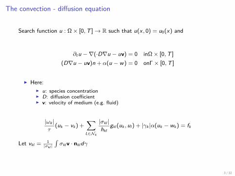
The convection - diffusion equation

Search function u : Ω× [0,T ]→ R such that u(x , 0) = u0(x) and

∂tu −∇(·D∇u − uv) = 0 inΩ× [0,T ]

(D∇u − uv)n + α(u − w) = 0 onΓ× [0,T ]

I Here:I u: species concentrationI D: diffusion coefficientI v: velocity of medium (e.g. fluid)

|ωk |τ

(uk − vk ) +∑

L∈Nk

|σkl |hkl

gkl (uk , ul ) + |γk |α(uk − wk ) = fk

Let vkl = 1|σkl |

∫σklv · nkldγ

3 / 32

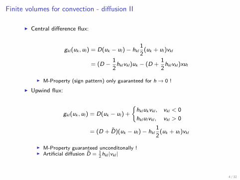
Finite volumes for convection - diffusion II

I Central difference flux:

gkl (uk , ul ) = D(uk − ul )− hkl12 (uk + ul )vkl

= (D − 12hklvkl )uk − (D +

12hklvkl )xul

I M-Property (sign pattern) only guaranteed for h→ 0 !I Upwind flux:

gkl (uk , ul ) = D(uk − ul ) +

hklukvkl , vkl < 0hklulvkl , vkl > 0

= (D + D)(uk − ul )− hkl12 (uk + ul )vkl

I M-Property guaranteed unconditonally !I Artificial diffusion D = 1

2hkl |vkl |

4 / 32

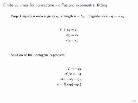
Finite volumes for convection - diffusion: exponential fitting

Project equation onto edge xK xL of length h = hkl , integrate once - q = −vkl

c ′ + cq = jc|0 = cK

c|h = cL

Solution of the homogeneus problem:

c ′ = −cqc ′/c = −q

ln c = c0 − qxc = K exp(−qx)

5 / 32

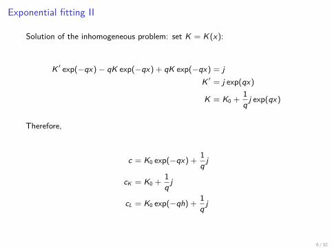
Exponential fitting II

Solution of the inhomogeneous problem: set K = K(x):

K ′ exp(−qx)− qK exp(−qx) + qK exp(−qx) = jK ′ = j exp(qx)

K = K0 +1q j exp(qx)

Therefore,

c = K0 exp(−qx) +1q j

cK = K0 +1q j

cL = K0 exp(−qh) +1q j

6 / 32

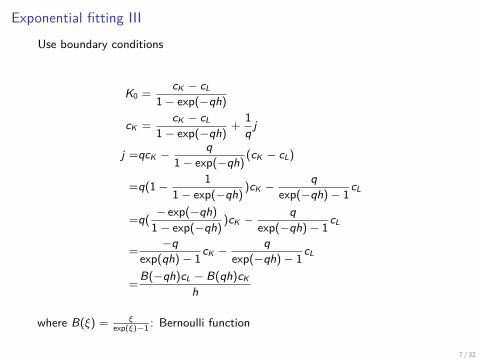
Exponential fitting III

Use boundary conditions

K0 =cK − cL

1− exp(−qh)

cK =cK − cL

1− exp(−qh)+

1q j

j =qcK −q

1− exp(−qh)(cK − cL)

=q(1− 11− exp(−qh)

)cK −q

exp(−qh)− 1cL

=q(− exp(−qh)

1− exp(−qh))cK −

qexp(−qh)− 1cL

=−q

exp(qh)− 1cK −q

exp(−qh)− 1cL

=B(−qh)cL − B(qh)cK

h

where B(ξ) = ξexp(ξ)−1 : Bernoulli function

7 / 32

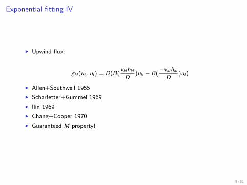
Exponential fitting IV

I Upwind flux:

gkl (uk , ul ) = D(B(vklhkl

D )uk − B(−vklhkl

D )ul )

I Allen+Southwell 1955I Scharfetter+Gummel 1969I Ilin 1969I Chang+Cooper 1970I Guaranteed M property!

8 / 32

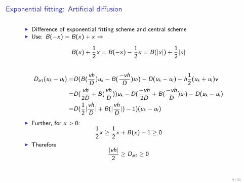
Exponential fitting: Artificial diffusion

I Difference of exponential fitting scheme and central schemeI Use: B(−x) = B(x) + x ⇒

B(x) +12x = B(−x)− 1

2x = B(|x |) +12 |x |

Dart(uk − ul ) =D(B(vhD )uk − B(

−vhD )ul )− D(uk − ul ) + h12 (uk + ul )v

=D(vh2D + B(

vhD ))uk − D(

−vh2D + B(

−vhD )ul )− D(uk − ul )

=D(12 |

vhD |+ B(|vh

D |)− 1)(uk − ul )

I Further, for x > 0:12x ≥ 1

2x + B(x)− 1 ≥ 0

I Therefore|vh|2 ≥ Dart ≥ 0

9 / 32

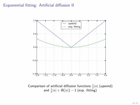
Exponential fitting: Artificial diffusion II

2.0 1.5 1.0 0.5 0.0 0.5 1.0 1.5 2.01.0

0.5

0.0

0.5

1.0

upwindexp. fitting

Comparison of artificial diffusion functions 12 |x | (upwind)

and 12 |x |+ B(|x |)− 1 (exp. fitting)

10 / 32

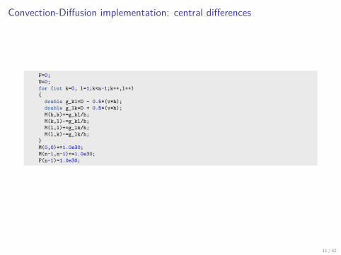
Convection-Diffusion implementation: central differences

F=0;U=0;for (int k=0, l=1;k<n-1;k++,l++)

double g_kl=D - 0.5*(v*h);double g_lk=D + 0.5*(v*h);M(k,k)+=g_kl/h;M(k,l)-=g_kl/h;M(l,l)+=g_lk/h;M(l,k)-=g_lk/h;

M(0,0)+=1.0e30;M(n-1,n-1)+=1.0e30;F(n-1)=1.0e30;

11 / 32

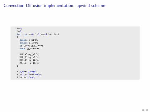
Convection-Diffusion implementation: upwind scheme

F=0;U=0;for (int k=0, l=1;k<n-1;k++,l++)

double g_kl=D;double g_lk=D;if (v<0) g_kl-=v*h;else g_lk+=v*h;

M(k,k)+=g_kl/h;M(k,l)-=g_kl/h;M(l,l)+=g_lk/h;M(l,k)-=g_lk/h;

M(0,0)+=1.0e30;M(n-1,n-1)+=1.0e30;F(n-1)=1.0e30;

12 / 32

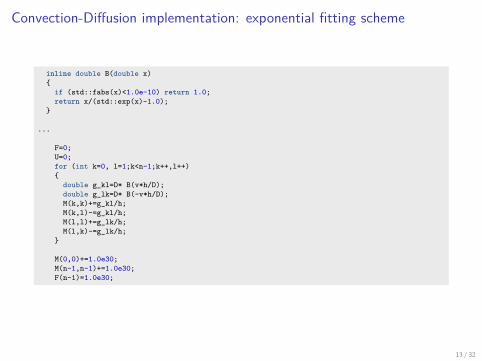
Convection-Diffusion implementation: exponential fitting scheme

inline double B(double x)

if (std::fabs(x)<1.0e-10) return 1.0;return x/(std::exp(x)-1.0);

...

F=0;U=0;for (int k=0, l=1;k<n-1;k++,l++)

double g_kl=D* B(v*h/D);double g_lk=D* B(-v*h/D);M(k,k)+=g_kl/h;M(k,l)-=g_kl/h;M(l,l)+=g_lk/h;M(l,k)-=g_lk/h;

M(0,0)+=1.0e30;M(n-1,n-1)+=1.0e30;F(n-1)=1.0e30;

13 / 32

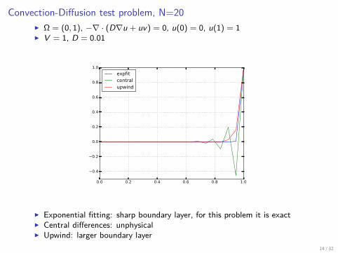
Convection-Diffusion test problem, N=20I Ω = (0, 1), −∇ · (D∇u + uv) = 0, u(0) = 0, u(1) = 1I V = 1, D = 0.01

0.0 0.2 0.4 0.6 0.8 1.0

0.4

0.2

0.0

0.2

0.4

0.6

0.8

1.0

expfitcentralupwind

I Exponential fitting: sharp boundary layer, for this problem it is exactI Central differences: unphysicalI Upwind: larger boundary layer

14 / 32

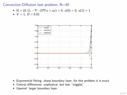
Convection-Diffusion test problem, N=40I Ω = (0, 1), −∇ · (D∇u + uv) = 0, u(0) = 0, u(1) = 1I V = 1, D = 0.01

0.0 0.2 0.4 0.6 0.8 1.0

0.4

0.2

0.0

0.2

0.4

0.6

0.8

1.0

expfitcentralupwind

I Exponential fitting: sharp boundary layer, for this problem it is exactI Central differences: unphysical, but less ‘’wiggles”I Upwind: larger boundary layer

15 / 32

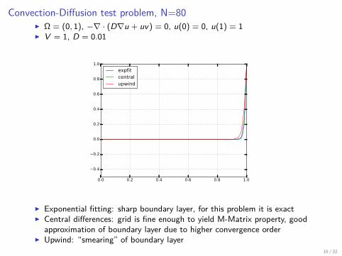
Convection-Diffusion test problem, N=80I Ω = (0, 1), −∇ · (D∇u + uv) = 0, u(0) = 0, u(1) = 1I V = 1, D = 0.01

0.0 0.2 0.4 0.6 0.8 1.0

0.4

0.2

0.0

0.2

0.4

0.6

0.8

1.0

expfitcentralupwind

I Exponential fitting: sharp boundary layer, for this problem it is exactI Central differences: grid is fine enough to yield M-Matrix property, good

approximation of boundary layer due to higher convergence orderI Upwind: “smearing” of boundary layer

16 / 32

1D convection diffusion summary

I upwinding and exponential fitting unconditionally yield the M-property ofthe discretization matrix

I exponential fitting for this case (zero right hand side, 1D) yields exactsolution. It is anyway “less diffusive” as artificial diffusion is optimized

I central scheme has higher convergence order than upwind (and exponentialfitting) but on coarse grid it may lead to unphysical oscillations

I for 2/3D problems, sufficiently fine grids to stabilize central scheme may beprohibitively expensive

I local grid refinement may help to offset artificial diffusion

17 / 32

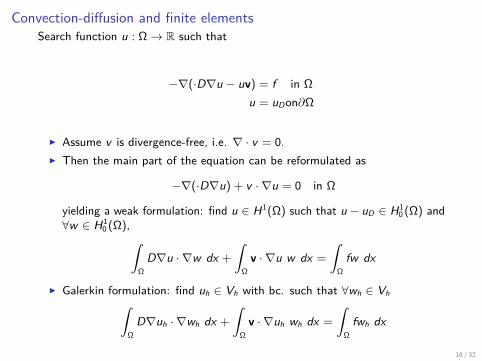
Convection-diffusion and finite elementsSearch function u : Ω→ R such that

−∇(·D∇u − uv) = f in Ω

u = uDon∂Ω

I Assume v is divergence-free, i.e. ∇ · v = 0.I Then the main part of the equation can be reformulated as

−∇(·D∇u) + v · ∇u = 0 in Ω

yielding a weak formulation: find u ∈ H1(Ω) such that u − uD ∈ H10 (Ω) and

∀w ∈ H10 (Ω),∫

Ω

D∇u · ∇w dx +

∫Ω

v · ∇u w dx =

∫Ω

fw dx

I Galerkin formulation: find uh ∈ Vh with bc. such that ∀wh ∈ Vh∫Ω

D∇uh · ∇wh dx +

∫Ω

v · ∇uh wh dx =

∫Ω

fwh dx

18 / 32

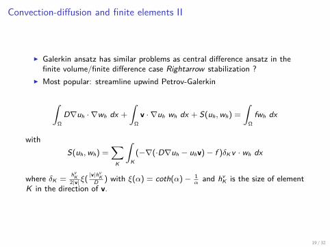
Convection-diffusion and finite elements II

I Galerkin ansatz has similar problems as central difference ansatz in thefinite volume/finite difference case Rightarrow stabilization ?

I Most popular: streamline upwind Petrov-Galerkin

∫Ω

D∇uh · ∇wh dx +

∫Ω

v · ∇uh wh dx + S(uh,wh) =

∫Ω

fwh dx

withS(uh,wh) =

∑K

∫K

(−∇(·D∇uh − uhv)− f )δK v · wh dx

where δK =hv

K2|v|ξ(

|v|hvK

D ) with ξ(α) = coth(α)− 1αand hv

K is the size of elementK in the direction of v.

19 / 32

Convection-diffusion and finite elements III

I Many methods to stabilize, none guarantees M-Property even on weaklyacute meshes ! (V. John, P. Knobloch, Computer Methods in AppliedMechanics and Engineering, 2007)

I Comparison paper:

M. Augustin, A. Caiazzo, A. Fiebach, J. Fuhrmann, V. John, A. Linke, and R.Umla, “An assessment of discretizations for convection-dominatedconvection-diffusion equations,” Comp. Meth. Appl. Mech. Engrg., vol. 200, pp.3395–3409, 2011:

I Topic of ongoing research

20 / 32

~

Nonlinear problems

21 / 32

Nonlinear problems: motivation

I Assume nonlinear dependency of some coefficients of the equation on thesolution. E.g. nonlinear diffusion problem

−∇(·D(u)∇u) = f in Ω

u = uDon∂Ω

I FE+FV discretization methods lead to large nonlinear systems of equations

22 / 32

Nonlinear problems: caution!

This is a significantly more complex world:

I Possibly multiple solution branchesI Weak formulations in Lp spacesI No direct solution methodsI Narrow domains of definition (e.g. only for positive solutions)

23 / 32

Finite element discretization for nonlinear diffusion

I Find uh ∈ Vh such that for all wh ∈ Vh:∫Ω

D(uh)∇uh · ∇wh dx =

∫Ω

fwh dx

I Use appropriate quadrature rules for the nonlinear integralsI Discrete system

A(uh) = F (uh)

24 / 32

Finite volume discretization for nonlinear diffusion

0 =

∫ωk

(−∇ · D(u)∇u − f ) dω

= −∫∂ωk

D(u)∇u · nkdγ −∫ωk

fdω (Gauss)

= −∑

L∈Nk

∫σkl

D(u)∇u · nkldγ −∫γk

D(u)∇u · ndγ −∫ωk

fdω

≈∑

L∈Nk

σkl

hklgkl (uk , ul ) + |γk |α(uk − vk )− |ωk |fk

with

gkl (uk , ul ) =

D( 1

2 (uk + ul ))(uk − ul )

orD(uk )−D(ul )

where D(u) =∫ u0 D(ξ) dξ (from exact solution ansatz at discretization edge)

I Discrete systemA(uh) = F (uh)

25 / 32

Iterative solution methods: fixed point iteration

I Let u ∈ Rn.I Problem: A(u) = f :

Assume A(u) = M(u)u, where for each u, M(u) : Rn → Rn is a linear operator.

I Fixed point iteration scheme:1. Choose initial value u0, i ← 02. For i ≥ 0, solve M(ui )ui+1 = f3. Set i ← i + 14. Repeat from 2) until converged

I Convergence criteria:I residual based: ||A(u)− f || < εI update based ||ui+1 − ui || < ε

I Large domain of convergenceI Convergence may be slowI Smooth coefficients not necessary

26 / 32

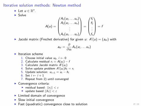
Iterative solution methods: Newton methodI Let u ∈ Rn.I Solve

A(u) =

A1(u1 . . . un)A2(u1 . . . un)

...An(u1 . . . un)

=

f1f2...fn

= f

I Jacobi matrix (Frechet derivative) for given u: A′(u) = (akl ) with

akl =∂

∂ulAk (u1 . . . un)

I Iteration scheme1. Choose initial value u0, i ← 02. Calculate residual ri = A(ui )− f3. Calculate Jacobi matrix A′(ui )4. Solve update problem A′(ui )hi = ri5. Update solution: ui+1 = ui − hi6. Set i ← i + 17. Repeat from 2) until converged

I Convergence criteria:I residual based: ||ri || < εI update based ||hi || < ε

I Limited domain of convergenceI Slow initial convergenceI Fast (quadratic) convergence close to solution 27 / 32

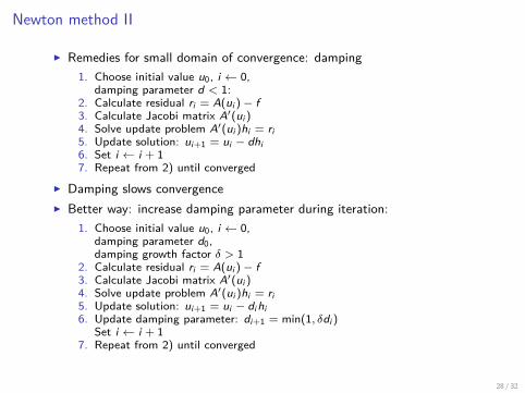
Newton method II

I Remedies for small domain of convergence: damping1. Choose initial value u0, i ← 0,

damping parameter d < 1:2. Calculate residual ri = A(ui )− f3. Calculate Jacobi matrix A′(ui )4. Solve update problem A′(ui )hi = ri5. Update solution: ui+1 = ui − dhi6. Set i ← i + 17. Repeat from 2) until converged

I Damping slows convergenceI Better way: increase damping parameter during iteration:

1. Choose initial value u0, i ← 0,damping parameter d0,damping growth factor δ > 1

2. Calculate residual ri = A(ui )− f3. Calculate Jacobi matrix A′(ui )4. Solve update problem A′(ui )hi = ri5. Update solution: ui+1 = ui − di hi6. Update damping parameter: di+1 = min(1, δdi )

Set i ← i + 17. Repeat from 2) until converged

28 / 32

Newton method III

I Even if it converges, in each iteration step we have to solve linear system ofequations

I can be done iteratively, e.g. with the LU factorization of the Jacobi matrixfrom first solution step

I iterative solution accuracy my be relaxed, but this may diminuish quadraticconvergence

I Quadratic convergence yields very accurate solution with no large additionaleffort: once we are in the quadratic convergence region, convergence is veryfast

I Monotonicity test: check if residual grows, this is often an sign that theiteration will diverge anyway.

29 / 32

Newton method IV

I Embedding method for parameter dependent problems.I Solve A(uλ, λ) = f for λ = 1.I Assume A(u0, 0) can be easily solved.I Parameter embedding method:

1. Solve A(u0, 0) = fchoose step size δ Set λ = 0

2. Solve A(uλ+δ, λ+ δ) = 0 with initial value uλ. Possibly decrease δ toachieve convergence

3. Set λ← λ+ δ4. Possibly increase δ5. Repeat from 2) until λ = 1

I Parameter embedding + damping + update based convergence control go along way to solve even strongly nonlinear problems!

30 / 32

~

Finite volume local stiffness matrix calculation

31 / 32

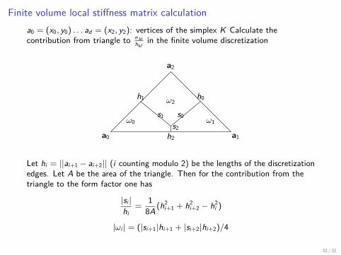
Finite volume local stiffness matrix calculationa0 = (x0, y0) . . . ad = (x2, y2): vertices of the simplex K Calculate thecontribution from triangle to σkl

hklin the finite volume discretization

a0

a2

a1

s2s0s1

ω2

ω0 ω1

h2

h1 h0

Let hi = ||ai+1 − ai+2|| (i counting modulo 2) be the lengths of the discretizationedges. Let A be the area of the triangle. Then for the contribution from thetriangle to the form factor one has

|si |hi

=18A (h2

i+1 + h2i+2 − h2

i )

|ωi | = (|si+1|hi+1 + |si+2|hi+2)/4

32 / 32