Euler systems for higher K-theory of number elds
34
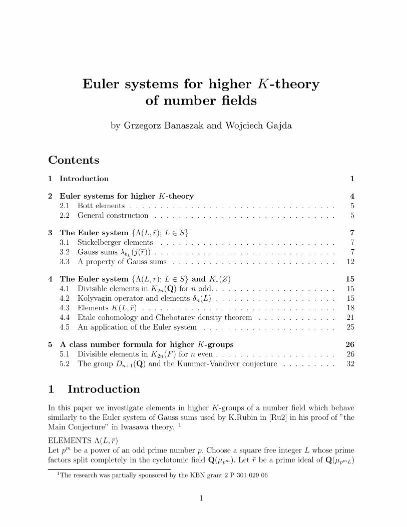
Euler systems for higher K -theory of number fields by Grzegorz Banaszak and Wojciech Gajda Contents 1 Introduction 1 2 Euler systems for higher K -theory 4 2.1 Bott elements .................................. 5 2.2 General construction .............................. 5 3 The Euler system {Λ(L, ¯ r); L ∈ S } 7 3.1 Stickelberger elements ............................. 7 3.2 Gauss sums λ b L (j ( r)) .............................. 7 3.3 A property of Gauss sums ........................... 12 4 The Euler system {Λ(L, ¯ r); L ∈ S } and K * (Z ) 15 4.1 Divisible elements in K 2n (Q) for n odd. .................... 15 4.2 Kolyvagin operator and elements δ n (L) .................... 15 4.3 Elements K (L, ¯ r) ................................ 18 4.4 Etale cohomology and Chebotarev density theorem ............. 21 4.5 An application of the Euler system ...................... 25 5 A class number formula for higher K -groups 26 5.1 Divisible elements in K 2n (F ) for n even .................... 26 5.2 The group D n+1 (Q) and the Kummer-Vandiver conjecture ......... 32 1 Introduction In this paper we investigate elements in higher K -groups of a number field which behave similarly to the Euler system of Gauss sums used by K.Rubin in [Ru2] in his proof of ”the Main Conjecture” in Iwasawa theory. 1 ELEMENTS Λ(L, ¯ r) Let p m be a power of an odd prime number p. Choose a square free integer L whose prime factors split completely in the cyclotomic field Q(μ p m). Let ¯ r be a prime ideal of Q(μ p m L ) 1 The research was partially sponsored by the KBN grant 2 P 301 029 06 1
Transcript of Euler systems for higher K-theory of number elds
Euler systems for higher K-theory
of number fields
by Grzegorz Banaszak and Wojciech Gajda
Contents
1 Introduction 1
2 Euler systems for higher K-theory 42.1 Bott elements . . . . . . . . . . . . . . . . . . . . . . . . . . . . . . . . . . 52.2 General construction . . . . . . . . . . . . . . . . . . . . . . . . . . . . . . 5
3 The Euler system {Λ(L, r); L ∈ S} 73.1 Stickelberger elements . . . . . . . . . . . . . . . . . . . . . . . . . . . . . 73.2 Gauss sums λbL(j(r)) . . . . . . . . . . . . . . . . . . . . . . . . . . . . . . 73.3 A property of Gauss sums . . . . . . . . . . . . . . . . . . . . . . . . . . . 12
4 The Euler system {Λ(L, r); L ∈ S} and K∗(Z) 154.1 Divisible elements in K2n(Q) for n odd. . . . . . . . . . . . . . . . . . . . . 154.2 Kolyvagin operator and elements δn(L) . . . . . . . . . . . . . . . . . . . . 154.3 Elements K(L, r) . . . . . . . . . . . . . . . . . . . . . . . . . . . . . . . . 184.4 Etale cohomology and Chebotarev density theorem . . . . . . . . . . . . . 214.5 An application of the Euler system . . . . . . . . . . . . . . . . . . . . . . 25
5 A class number formula for higher K-groups 265.1 Divisible elements in K2n(F ) for n even . . . . . . . . . . . . . . . . . . . . 265.2 The group Dn+1(Q) and the Kummer-Vandiver conjecture . . . . . . . . . 32
1 Introduction
In this paper we investigate elements in higher K-groups of a number field which behavesimilarly to the Euler system of Gauss sums used by K.Rubin in [Ru2] in his proof of ”theMain Conjecture” in Iwasawa theory. 1
ELEMENTS Λ(L, r)Let pm be a power of an odd prime number p. Choose a square free integer L whose primefactors split completely in the cyclotomic field Q(µpm). Let r be a prime ideal of Q(µpmL)
1The research was partially sponsored by the KBN grant 2 P 301 029 06
1
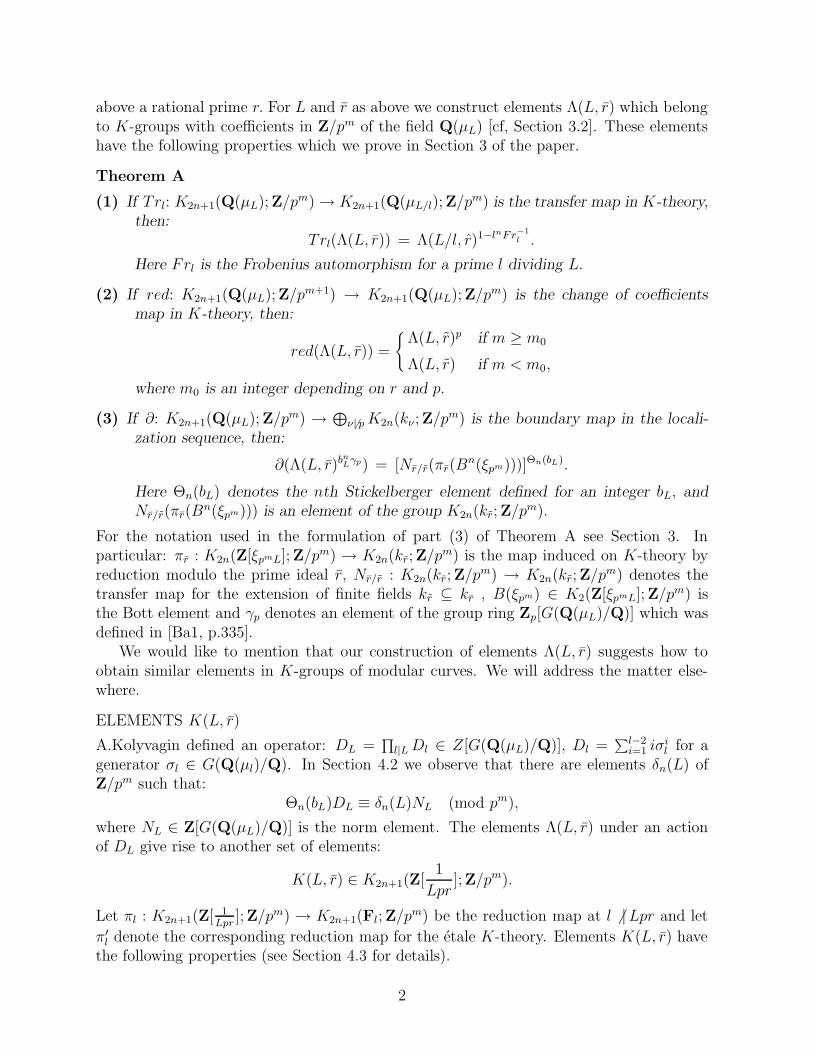
above a rational prime r. For L and r as above we construct elements Λ(L, r) which belongto K-groups with coefficients in Z/pm of the field Q(µL) [cf, Section 3.2]. These elementshave the following properties which we prove in Section 3 of the paper.
Theorem A
(1) If Trl: K2n+1(Q(µL); Z/pm) → K2n+1(Q(µL/l); Z/pm) is the transfer map in K-theory,
then:
Trl(Λ(L, r)) = Λ(L/l, r)1−lnFr−1l .
Here Frl is the Frobenius automorphism for a prime l dividing L.
(2) If red: K2n+1(Q(µL); Z/pm+1) → K2n+1(Q(µL); Z/pm) is the change of coefficients
map in K-theory, then:
red(Λ(L, r)) =
{Λ(L, r)p if m ≥ m0
Λ(L, r) if m < m0,
where m0 is an integer depending on r and p.
(3) If ∂: K2n+1(Q(µL); Z/pm) → ⊕ν 6| pK2n(kν; Z/p
m) is the boundary map in the locali-
zation sequence, then:
∂(Λ(L, r)bnLγp) = [Nr/r(πr(B
n(ξpm)))]Θn(bL).
Here Θn(bL) denotes the nth Stickelberger element defined for an integer bL, and
Nr/r(πr(Bn(ξpm))) is an element of the group K2n(kr; Z/p
m).
For the notation used in the formulation of part (3) of Theorem A see Section 3. Inparticular: πr : K2n(Z[ξpmL]; Z/pm) → K2n(kr; Z/p
m) is the map induced on K-theory byreduction modulo the prime ideal r, Nr/r : K2n(kr; Z/p
m) → K2n(kr; Z/pm) denotes the
transfer map for the extension of finite fields kr ⊆ kr , B(ξpm) ∈ K2(Z[ξpmL]; Z/pm) isthe Bott element and γp denotes an element of the group ring Zp[G(Q(µL)/Q)] which wasdefined in [Ba1, p.335].
We would like to mention that our construction of elements Λ(L, r) suggests how toobtain similar elements in K-groups of modular curves. We will address the matter else-where.
ELEMENTS K(L, r)
A.Kolyvagin defined an operator: DL =∏l|LDl ∈ Z[G(Q(µL)/Q)], Dl =
∑l−2i=1 iσ
il for a
generator σl ∈ G(Q(µl)/Q). In Section 4.2 we observe that there are elements δn(L) ofZ/pm such that:
Θn(bL)DL ≡ δn(L)NL (mod pm),
where NL ∈ Z[G(Q(µL)/Q)] is the norm element. The elements Λ(L, r) under an actionof DL give rise to another set of elements:
K(L, r) ∈ K2n+1(Z[1
Lpr]; Z/pm).
Let πl : K2n+1(Z[ 1Lpr
]; Z/pm) → K2n+1(Fl; Z/pm) be the reduction map at l 6 |Lpr and let
π′l denote the corresponding reduction map for the etale K-theory. Elements K(L, r) havethe following properties (see Section 4.3 for details).
2
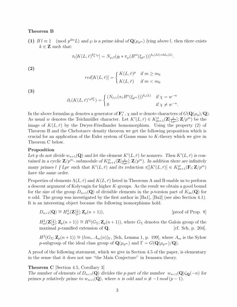
Theorem B
(1) If l ≡ 1 (mod p2mL) and ℘ is a prime ideal of Q(µpm) lying above l, then there exists
k ∈ Z such that:
πl[K(L, r)bnLγp] = N℘/l(gl ∗ π℘(Bm(ξpn)))δn(Ll)+kδn(L).
(2)
red[K(L, r)] =
{K(L, r)p if m ≥ m0
K(L, r) if m < m0
(3)
∂r(K(L, r)γpbnL) =
{(Nr/r(πrB
n(ξpm)))δn(L) if χ = w−n
0 if χ 6= w−n.
In the above formulas gl denotes a generator of F×l , χ and w denote characters ofG(Q(µp)/Q).As usual w denotes the Teichmuller character. Let K ′(L, r) ∈ Ket
2n+1(Z[ 1Lpr
]; Z/pm) be the
image of K(L, r) by the Dwyer-Friedlander homomorphism. Using the property (2) ofTheorem B and the Chebotarev density theorem we get the following proposition which iscrucial for an application of the Euler system of Gauss sums to K-theory which we give inTheorem C below.
PropositionLet p do not divide wn+1(Q) and let the element K ′(L, r) be nonzero. Then K ′(L, r) is con-
tained in a cyclic Z/pm- submodule of Ket2n+1(Z[ 1
Lpr]; Z/pm). In addition there are infinitely
many primes l 6 | Lpr such that K ′(L, r) and its reduction π′l[K′(L, r)] ∈ Ket
2n+1(Fl; Z/pm)
have the same order.
Properties of elements Λ(L, r) and K(L, r) listed in Theorems A and B enable us to performa descent argument of Kolyvagin for higher K-groups. As the result we obtain a good boundfor the size of the group Dn+1(Q) of divisible elements in the p-torsion part of K2n(Q) forn odd. The group was investigated by the first author in [Ba1], [Ba2] (see also Section 4.1).It is an interesting object because the following isomorphisms hold.
Dn+1(Q) ∼= H2et(Z[1
p]; Zp(n+ 1)), [proof of Prop. 8]
H2et(Z[1
p]; Zp(n+ 1)) ∼= H2(GΣ; Zp(n+ 1)), where GΣ denotes the Galois group of the
maximal p-ramified extension of Q, [cf. Sch, p. 204].
H2(GΣ; Zp(n+ 1)) ∼= (lim←Am(n))Γ, [Sch, Lemma 1, p. 199], where Am is the Sylowp-subgroup of the ideal class group of Q(µpm) and Γ = G(Q(µp∞)/Q).
A proof of the following statement, which we give in Section 4.5 of the paper, is elementaryin the sense that it does not use “the Main Conjecture” in Iwasawa theory.
Theorem C [Section 4.5, Corollary 3]The number of elements of Dn+1(Q) divides the p-part of the number wn+1(Q)ζQ(−n) for
primes p relatively prime to wn+1(Q), where n is odd and n 6≡ −1mod (p− 1).
3
Let us point out that the first author and M.Kolster in [Ba2, Theorem 3] obtained a strongerresult which implies equality of the numbers appearing in Theorem C but in the proof theyhad to apply ”the Main Conjecture”. While proving Theorem C we generalized some ofRubin’s results from [Ru2] for the field Q(µpm) and m > 1, e.g., Theorem 1 in Section4.3. All the computations in Section 4 show a striking analogy between arithmetic of classgroups of cyclotomic fields and arithmetic of the group Dn+1(Q). More on the analogy maybe found in [Ba2, p.292].
In the last section of the paper we prove some results about the group Dn+1(F ) for anumber field F in the case when n is even. We generalize a theorem of Bloch and Kato[BK, (6.6), p.385] and obtain an index formula for the number of divisible elements whenF is totally real, abelian. The proof uses ”the Main Cojecture.” We were informed thatM.Kolster, T.Nguyen Quang Do and M.Fleckinger have obtained a similar formula to ourTheorem D, [KNF, Cor. 5.7, p. 27].
Theorem DIf F is a totally real, abelian number field and p does not divide the conductor of F, then
we have the following formula for the number of elements in Dn+1(F ).
|Dn+1(F )| = [Ket2n+1(OF [
1
p]) ; Cet
2n+1]
Here Cet2n+1 stands for the image in etale K-theory of Soule’s group of cyclotomic elements
defined for the field F.
We think that the formula is an analogue for higher K-groups of the field F of theclassical Kummer formula for the second factor of the class number of the cyclotomic field[La, Theorem 5.1, p.85]. In Section 5.2 of the paper using results of M.Kurihara [Ku] wereformulate the Kummer-Vandiver conjecture in terms of the groups Dn+1(Q) (n even).Recall from [Ba2] that the Quillen-Lichtenbaum conjecture for K2n(Z) (n odd) has anequivalent statement using Dn+1(Q).
Acknowledgements
The first author would like to thank Manfred Kolster and Victor Snaith for all help
and support during his work at McMaster University where his part of this paper has been
written. In addition, he would like to thank the Swiss National Science Foundation and
the University of Lausanne for their hospitality during November 1993.
The second author would like to thank SFB 343 “Diskrete Strukturen in der Mathe-
matik” at the University of Bielefeld, where this paper has been completed, for the invita-
tion and hospitality. He also wants to express his gratitude to Rainer Vogt and Friedhelm
Waldhausen whose help over the years made this work possible.
2 Euler systems for higher K-theory
Euler systems introduced by A.Kolyvagin and K.Rubin may be used to construct interestingsystems of elements in algebraic K-theory. Let F/Q be an abelian field extension. We fixan odd prime p and a natural number m. Let S be the set of square free natural numbers
4
such that they are divisible only by primes l that split completely in F and such thatl ≡ 1mod pm. We will use Euler systems as in [Ru3].
Definition 1 Let α(L) ∈ F (µpmL) for L ∈ S be elements satisfying:
(1) α(L) ∈ F (µpmL)× so α(L) 6= 0
(2) if l|L then Nl(α(L)) ≡ (Frl − 1)α(L/l) mod F (µpm(L/l))×M or
(2’) if l|L then Nl(α(L)) ≡ (1 − Fr−1l )α(L/l) mod F (µpm(L/l))
×M , where M is a naturalnumber divisible by pm.
We call a set {α(L) ∈ F (µpmL); L ∈ S} with properties (1) and (2) or (1) and (2’) anEuler system for the field F.
Remark 1. α(L) depends on pm but pm is fixed so we do not denote it. Nl =∑σ ∈
Z[G(F (µpmL)/F (µpm(L/l)))] is the norm element and Frl ∈ G(F (µpm(L/l))/F ) is the Frobe-nius element which raises ξpm(L/l) to the lth power, [Ru, p. 310].
Remark 2. The Euler system of cyclotomic units denoted by ξr in [Ru1] satisfies conditions(1) and (2). The Euler system of Gauss sums from [Ru2] satisfies (1) and (2’).
2.1 Bott elements
Let A be a domain which contains a primitive root of unity of order pm denoted by ξpm. LetK∗(−; Z/pm) denote the K-theory with Z/pm coefficients defined by Browder and Karoubi.The Bockstein exact sequence in K-theory gives the following exact sequence.
K2(A; Z/pm) → K1(A)[pm] → 0
Observe that: K1(A)[pm] = A∗[pm]. In [So1] C.Soule shows that there is a canonical Bottelement B(ξpm) ∈ K2(A; Z/pm) (denoted by αn in [So1]) such that ξpm is the image ofB(ξpm) by the surjective map of the above exact sequence. By definition B(ξpm) is theimage of ξpm by the following composition of maps. Let µpm denote the group of pmth rootsof unity.
µpm
∼=−→ π1(BGL1(A))[pm]∼=−→ π2(BGL1(A); Z/pm) → K2(A; Z/pm)
Observe that if ϕ : A→ A is a ring homomorphism, then we have: B(ϕ(ξpm)) = ϕ(B(ξpm)).But ϕ(ξpm) = ξcpm for some c ∈ Z, hence ϕ(B(ξpm)) = B(ξpm)c. If A is the ring of integers ina number field and ℘ is its prime ideal such that ℘ does not divide p, then π℘(B(ξpm)) is theBott element in the cyclic group K2(k℘; Z/pm). Here π℘ : K2(A; Z/pm) → K2(k℘; Z/pm)denotes the reduction map on K-groups.
2.2 General construction
Note that by assumptions on p and L we have F (µpm)∩F (µL) = F for all L ∈ S. Let OpmL
denote the ring of integers in F (µpm, µL) and Opm denote the ring of integers in F (µpm).
5
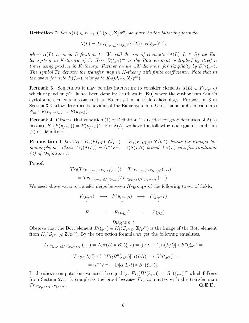
Definition 2 Let Λ(L) ∈ K2n+1(F (µL),Z/pm) be given by the following formula.
Λ(L) = TrF (µpmL)/F (µL)(α(L) ∗B(ξpm)∗n),
where α(L) is as in Definition 1. We call the set of elements {Λ(L); L ∈ S} an Eu-ler system in K-theory of F. Here B(ξpm)∗n is the Bott element multiplied by itself ntimes using product in K-theory. Further on we will denote it for simplicity by Bn(ξpm).The symbol Tr denotes the transfer map in K-theory with finite coefficients. Note that inthe above formula B(ξpm) belongs to K2(OpmL,Z/p
m).
Remark 3. Sometimes it may be also interesting to consider elements α(L) ∈ F (µpmL)which depend on pm. It has been done by Kurihara in [Ku] where the author uses Soule’scyclotomic elements to construct an Euler system in etale cohomology. Proposition 3 inSection 3.3 below describes behaviour of the Euler system of Gauss sums under norm mapsNm : F (µpm+1L) → F (µpmL).
Remark 4. Observe that condition (1) of Definition 1 is needed for good definition of Λ(L)because K1(F (µpmL)) = F (µpmL)×. For Λ(L) we have the following analogue of condition(2) of Definition 1.
Proposition 1 Let Trl : K∗(F (µL); Z/pm) → K∗(F (µL/l); Z/pm) denote the transfer ho-
momorphism. Then: Trl(Λ(L)) = (l−nFrl − 1)Λ(L/l) provided α(L) satisfies conditions(2) of Definition 1.
Proof.Trl(TrF (µpmL)/F (µL)(. . .)) = TrF (µpmL)/F (µL/l)(. . .) =
= TrF (µpmL/l)/F (µL/l)TrF (µpmL)/F (µpmL/l)(. . .).
We used above various transfer maps between K-groups of the following tower of fields.
F (µpm) −→ F (µpmL/l) −→ F (µpmL)x
xx
F −→ F (µL/l) −→ F (µL)
Diagram 1
Observe that the Bott element B(ξpm) ∈ K2(OpmL; Z/pm) is the image of the Bott elementfrom K2(OpmL/l; Z/p
m). By the projection formula we get the following equalities.
TrF (µpmL)/F (µpmL/l)(. . .) = Nlα(L) ∗Bn(ξpm) = [(Frl − 1)α(L/l)] ∗Bn(ξpm) =
= [Frlα(L/l) ∗ l−nFrlBn(ξpm)][α(L/l)−1 ∗Bn(ξpm)] =
= (l−nFrl − 1)[α(L/l) ∗Bn(ξpm)].
In the above computations we used the equality: Frl(Bn(ξpm)) = [Bn(ξpm)]l
nwhich follows
from Section 2.1. It completes the proof because Frl commutes with the transfer mapTrF (µpmL/l)/F (µL/l). Q.E.D.
6
Remark 5. If we used condition (2’) of Definition 1 in the last proposition, then we wouldget the following equality.
Trl(Λ(L)) = (1 − lnFr−1l )Λ(L/l)
Example. Putα(L) = (1 − ξpm
∏
l|L
ξl)(1 − ξ−1pm
∏
l|L
ξl).
These elements were used by K.Rubin. They satisfy conditions ES1.−ES4. of [Ru1]. Hencethey give well defined Euler system Λ(L) for higher K-groups in the sense of Definition 2.It is the Euler system whose image by the Dwyer-Friedlander map is the Euler system inetale cohomology of SpecZ[1/L] considered by Kurihara in [Ku, Section 5].
3 The Euler system {Λ(L, r); L ∈ S}3.1 Stickelberger elements
For convenience of the reader we recall from [Ba1, p. 328-329] definition of the higherStickelberger elements. Let F/Q be an abelian extension with conductor f. Let σa denotean automorphism of Q(µf ) such that for a root of unity ξ of order f one has: σa(ξ) = ξa.Denote by (a;F ) the restriction of σa to F. Let b be an integer which is relatively prime tothe number wn+1(Q(µf)). Define
Θn(b) = (bn+1 − (b;F ))∑
1≤a≤f, (a,f)=1
ζf(a,−n)(a;F )−1,
where ζf is the partial zeta function. Let us write the element Θn(b) as:
Θn(b) =∑
1≤a≤f, (a,f)=1
∆n+1(a, b, f)(a;F )−1.
By [CS, Theorem 1.2] we know that Θn(b) ∈ Z[G(F/Q)]. For F = Q (f = 1) we putΘn(b) = (bn+1 − 1)ζQ(−n), where ζQ is the Riemann zeta. By [CS, Theorem 3] we have:∆n+1(a, b, f) ≡ (ab)n∆1(a, b, f)mod f
∏p|f p
υp(n).
3.2 Gauss sums λbL(j(r))
The following section is based on the construction of map Λ from [Ba1]. We will use theEuler system of Gauss sums of K. Rubin from [Ru2] twisted by the Galois action. LetF be an abelian number field with conductor f . We pick a prime number r such that(r, fpmL) = 1. Choose a natural number bL such that (bL, wn+1(Q(µfpmL))) = 1. Letj : F (µpmL) → Q(µf) be the natural imbedding, where f is the conductor of F (µpmL). Weare going to use elements λbL(j(r)) from [C, p.308-309] whose definition is recalled belowfor the convenience of the reader.
7
Definition 3 Let ℘ be a prime ideal of Q(µf). Let εf ,℘ : k×℘ → µf be the character defined
by the congruence : εf ,℘(x) ≡ xN℘−1
f mod℘. Denote by ψ : k℘ → µp the additive characterψ(x) = ξp
trx. Define the Gauss sum:
G(εf ,℘;ψ) = Σx∈k℘εf ,℘(x)ψ(x).
Let now ℘ be a prime of Q(µf) which does not divide w1(Q(µf )). We put: τ(℘) =G(εf ,℘;ψ)√
(N℘)∗,
where N℘ = pr and
(N℘)∗ =
{pr if p ≡ 1 mod 4
(−p)r if p ≡ 1 mod 4.
For j(r) =∏℘|j(r) ℘
e℘ we put:
τ(j(r)) =∏
℘|j(r)
τ(℘)e℘.
We define the element λbL(j(r)) by the following formula.
λbL(j(r)) =τ(j(r))bL
τ(j(r)σbL )
Note that by [C, Prop. 3.8] (λbL(j(r))) = rΘ0(bL). We define elements Λ(L) = Λ(L, r) ∈K2n+1(F (µL); Z/pm) as in Definition 2 using α(L) = λbL(j(r)).
In the sequel we will use the following notation from [Ba1].
1. γp = 1 + pnσ−1p + p2nσ−2
p + . . . if p does not divide f . Put γp = 1 if p|f where σp wasintroduced in [Ba1, p.335].
2. r is a prime ideal in F (µpmL) over a rational prime r. r is the prime in F (µL) below r.
3. Nr/r : K2n(kr; Z/pm) → K2n(kr; Z/p
m) is the transfer homomorphism.
4. πr : K2n(OF (µpmL); Z/pm) → K2n(kr; Z/p
m) is the reduction map.
5. ∂ : K2n+1(F (µL); Z/pm) → ⊕vK2n(kv; Z/p
m) is the boundary map from the locali-zation sequence.
6. Θn(bL) is the higher Stickelberger element for F (µL).
7. Θ∗n(bL) is the higher Stickelberger element for F (µpmL).
Proposition 2∂(Λ(L, r)b
nLγp) = [Nr/r(πr(B
n(ξpm)))]Θn(bL)
Proof. Our proof follows main idea of the proof of [Ba1, Theorem 1]. We do a sketch of theproof. We want to point out that the proof of Theorem 1 of [Ba1] is not completely correct.The mistake will be removed in the present sketch. Consider the following commutativediagrams.
8
K2n+1(F (µpmL); Z/pm)∂′−→ ⊕
wK2n(kw; Z/pm)yTr
y⊕
w|vNw/v
K2n+1(F (µL); Z/pm)∂−→ ⊕
vK2n(kv; Z/pm)
Diagram 3.
Let O′ denote OF (µpmL) and let σ−1a = (a−1;F (µpmL)) = (a;F (µpmL))−1.
K2n(O′; Z/pm)πr−→ K2n(kr; Z/p
m)yσ−1
a
yσ−1a
K2n(O′; Z/pm)π
rσ−1a−→ K2n(k
rσ−1a
; Z/pm)
Diagram 4.
It follows from commutativity of Diagram 4 that: πrσ−1
a(Bn(ξpm)) = [πr(B
n(ξpm))]anσ−1
a .
The following diagram also commutes cf. Diagram 4.8 in [Ba1].
K2n(kr; Z/pm)
σ−1a−→ K2n(k
rσ−1a
; Z/pm)yNr/r
yNrσ−1a /rσ−1
a
K2n(kr; Z/pm)
σ−1a−→ K2n(k
rσ−1a
; Z/pm)
Diagram 5.
The equalities below follow from commutativity of Diagrams 3, 4 and 5.
∂(Λ(L, r)bnLγp) = [∂(Λ(L, r))]b
nLγp =
= [∂ ◦ TrF (µpmL)/F (µL)(α(L; r) ∗Bn(ξpm))]bnLγp =
= [N ◦ ∂′(α(L; r) ∗Bn(ξpm))]bnLγp = [N([πrB
n(ξpm)]Θ∗n(bL))]γp =
= [Nr/r ◦ πr(Bn(ξpm))]Θn(bL).
The mistake in [Ba1] was in computation of ∂ ′(...) above. The correction goes as follows.Let f (f) be the conductor of F (µpmL) (F (µL) resp.). We will compute the images of ∂ ′ foreach ω (a prime ideal of O′). First if ω = r take all c mod f such that: (c;F (µpmL))r = r.Because (c;F (µpmL)) is the restriction of σc to F (µpmL) we will continue to use the σcnotation. Observe that: Bn(ξpm)(c;F (µpmL)) = Bn(ξpm)c
ncf. Section 2.1.
∂′(α(L; r) ∗Bn(ξpm)) = (∑
cmodfrσc=r
∆1(c, bL, f))[kr] ∗ πr(Bn(ξpm)) =
= πr(Bn(ξpm))
∑cmodfrσc=r
∆1(c,bL,f)cnσ−1
c
.
Similarly if ω 6= r and ω = rσ−1a , then:
∂′(α(L; r) ∗Bn(ξpm)anσ−1
a ) = (∑
cmodfrσc=r
∆1(ac, bL, f))[krσ−1
a] ∗ π
rσ−1a
(Bn(ξpm)anσ−1
a ) =
9
= πr(Bn(ξpm))
∑cmodfrσc=r
∆1(ac,bL,f)cnanσ−1ac
.
If ω is not a G(Q(µf )/Q) conjugate of r, then ∂ ′(...) = 0. From now on the computationgoes as in [Ba1]. Q.E.D.
Let b be a positive integer such that (b, pmwn+1(Q(µf))) = 1. Put M = pm. Take Lsuch that and (L, bMwn+1(Q(µf)) = 1. For a moment we assume that F = Q(µf) and doall computations for this case. At the end of the section we will describe how to deal withthe general case. The following notation and comments will be useful in the proof of nextlemma.
1. Let be given a character:εL,r : k×r −→ µpmLf
such that εL,r(x) ≡ xNr−1pmLf mod r, and r denotes a prime ideal in F (µpmL) above r.
2. Let g(L, r, ξr) = G(εL,r;ψ) =∑x∈k∗
rεL,r(x)ξtr(x)r , [cf. Definition 3].
3. Observe that b is odd. We can choose a natural number bL such that
bL ≡ bmodwn+1(Q(µf ))pmML.
In this way σbL is an element of G(F (µpmL)/Q) whose restriction to G(F (µpm)/Q)is σb. Let σbL be the unique element of G(F (µpmLr)/Q(µr)) which restricts inG(F (µpmL)/Q) to σbL . Observe that bL is relatively prime to wn+1(Q(µpmLf )).
4. Let N(r) = rk. Then denote N(r)∗ = rk, ((−r)k resp.) if r ≡ 1 mod 4 (r ≡ 3 mod 4,
resp.). We know that Q(√N(r)∗) ⊂ Q(µr), [C, p. 308].
5. Assume that the prime ideal in F (µpm) below r splits completely in F (µpmL), e.g.,when r ≡ 1 mod L. Put r to be the prime ideal in F (µpm(L/l)) below r. Observe thatN(r) = N(r). Hence kr = kr and εlL,r = εL/l,r.
6. In the same way we define bL/l. In this way σbL/lis the restriction of σbL to F (µpmL/l).
We see that restriction of σbL to F (µpm(L/l)r) equals to σbL/l. In addition we have:
bL ≡ bL/lmod pmM(L/l)wn+1(Q(µf)).
7. Fix a natural number l′ such that:
ll′ ≡ 1mod fpm(L/l)r.
Lemma 1NlλbL(r) ≡ λbL/l
(r)1−Fr−1l modF (µpm(L/l))
×M
Proof. By [C, Lemma 3.10] we have:
Nl(λbL(r)) = Nl(g(L, r, ξr))bL−σbL (N(r)∗(l−1)(1−bL)/2).
10
But Nl(g(L, r, ξr))bL−σbL = [
∏σ∈Gl
(∑x∈k∗
rεL,r(x)σξtr(x)r )]bL−σbL =
= [∏
ϕ:k∗r→µl
(∑
x∈k∗r
ϕ(x)εL,r(x)ξtr(x)r )]bL−σbL [∑
x∈k∗r
εL,r(x)ll′
ξtr(x)r ]σbL−bL .
By Davenport-Hasse distribution relation [La] the last expression equals:
[(∑
x∈k∗r
εL/l,r(x)ξtr(x)r )]bL−σbL [εL,r(l)−l(−N(r)(l−1)/2)]bL−σbL ×
×[(∑
x∈k∗r
εL/l,r(x)ξtr(lx)r )−Fr−1l ]bL−σbL
which further equals:
[(∑
x∈k∗r
εL/l,r(x)ξtr(x)r )1−Fr−1l ]bL−σbL [εL/l,r(l)
l′−1]bL−σbL [N(r)(l−1)/2]bL−1.
So we have: Nl(λbL(r)) = [g(L/l, r, ξr)1−Fr−1
l ]bL−σbL =
= [g(L/l, r, ξr)1−Fr−1
l ]bL/l−σbL/l [(
√N(r)∗)
bL/l−σbL/l ]Fr−1l−1 ≡
≡ (λbL/l(r))1−Fr−1
l modF (µpm(L/l))×M
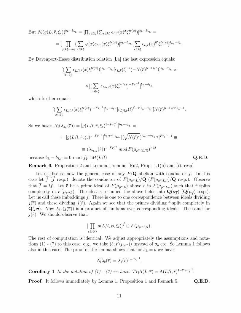
because bL − bL/l ≡ 0 mod fpmM(L/l) Q.E.D.
Remark 6. Proposition 2 and Lemma 1 remind [Ru2, Prop. 1.1(ii) and (i), resp].
Let us discuss now the general case of any F/Q abelian with conductor f . In thiscase let f (f resp.) denote the conductor of F (µpmL)/Q (F (µpmL/l)/Q resp.). Observe
that f = lf . Let r be a prime ideal of F (µpmL) above r in F (µpmL/l) such that r splitscompletely in F (µpmL). The idea is to imbed the above fields into Q(µf ) (Q(µf) resp.).Let us call these imbeddings j. There is one to one correspondence between ideals dividingj(r) and these dividing j(r). Again we see that the primes dividing r split completely inQ(µf). Now λbL(j(r)) is a product of lambdas over corresponding ideals. The same forj(r). We should observe that:
[∏
℘|j(r)
g(L/l, ℘, ξr)]f ∈ F (µpmL/l).
The rest of computation is identical. We adjust appropriately the assumptions and nota-tions (1) - (7) to this case, e.g., we take (b;F (µpm)) instead of σb etc. So Lemma 1 followsalso in this case. The proof of the lemma shows that for bL = b we have:
Nlλb(r) = λb(r)1−Fr−1
l .
Corollary 1 In the notation of (1) - (7) we have: TrlΛ(L, r) = Λ(L/l, r)1−lnFr−1l .
Proof. It follows immediately by Lemma 1, Proposition 1 and Remark 5. Q.E.D.
11
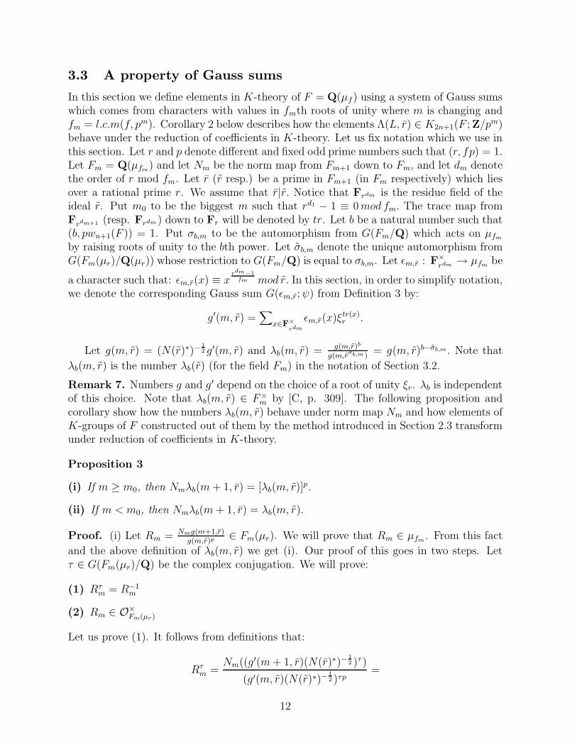
3.3 A property of Gauss sums
In this section we define elements in K-theory of F = Q(µf) using a system of Gauss sumswhich comes from characters with values in fmth roots of unity where m is changing andfm = l.c.m(f, pm). Corollary 2 below describes how the elements Λ(L, r) ∈ K2n+1(F ; Z/pm)behave under the reduction of coefficients in K-theory. Let us fix notation which we use inthis section. Let r and p denote different and fixed odd prime numbers such that (r, fp) = 1.Let Fm = Q(µfm) and let Nm be the norm map from Fm+1 down to Fm, and let dm denotethe order of r mod fm. Let r (r resp.) be a prime in Fm+1 (in Fm respectively) which liesover a rational prime r. We assume that r|r. Notice that Frdm is the residue field of theideal r. Put m0 to be the biggest m such that rd1 − 1 ≡ 0mod fm. The trace map fromFrdm+1 (resp. Frdm ) down to Fr will be denoted by tr. Let b be a natural number such that(b, pwn+1(F )) = 1. Put σb,m to be the automorphism from G(Fm/Q) which acts on µfm
by raising roots of unity to the bth power. Let σb,m denote the unique automorphism fromG(Fm(µr)/Q(µr)) whose restriction to G(Fm/Q) is equal to σb,m. Let εm,r : F×rdm → µfm be
a character such that: εm,r(x) ≡ xrdm−1
fm mod r. In this section, in order to simplify notation,we denote the corresponding Gauss sum G(εm,r;ψ) from Definition 3 by:
g′(m, r) =∑
x∈F×
rdm
εm,r(x)ξtr(x)r .
Let g(m, r) = (N(r)∗)−12 g′(m, r) and λb(m, r) = g(m,r)b
g(m,rσb,m)
= g(m, r)b−σb,m . Note that
λb(m, r) is the number λb(r) (for the field Fm) in the notation of Section 3.2.
Remark 7. Numbers g and g′ depend on the choice of a root of unity ξr. λb is independentof this choice. Note that λb(m, r) ∈ F×m by [C, p. 309]. The following proposition andcorollary show how the numbers λb(m, r) behave under norm map Nm and how elements ofK-groups of F constructed out of them by the method introduced in Section 2.3 transformunder reduction of coefficients in K-theory.
Proposition 3
(i) If m ≥ m0, then Nmλb(m+ 1, r) = [λb(m, r)]p.
(ii) If m < m0, then Nmλb(m + 1, r) = λb(m, r).
Proof. (i) Let Rm = Nmg(m+1,r)g(m,r)p ∈ Fm(µr). We will prove that Rm ∈ µfm . From this fact
and the above definition of λb(m, r) we get (i). Our proof of this goes in two steps. Letτ ∈ G(Fm(µr)/Q) be the complex conjugation. We will prove:
(1) Rτm = R−1
m
(2) Rm ∈ O×Fm(µr)
Let us prove (1). It follows from definitions that:
Rτm =
Nm((g′(m+ 1, r)(N(r)∗)−12 )τ )
(g′(m, r)(N(r)∗)−12 )τp
=
12
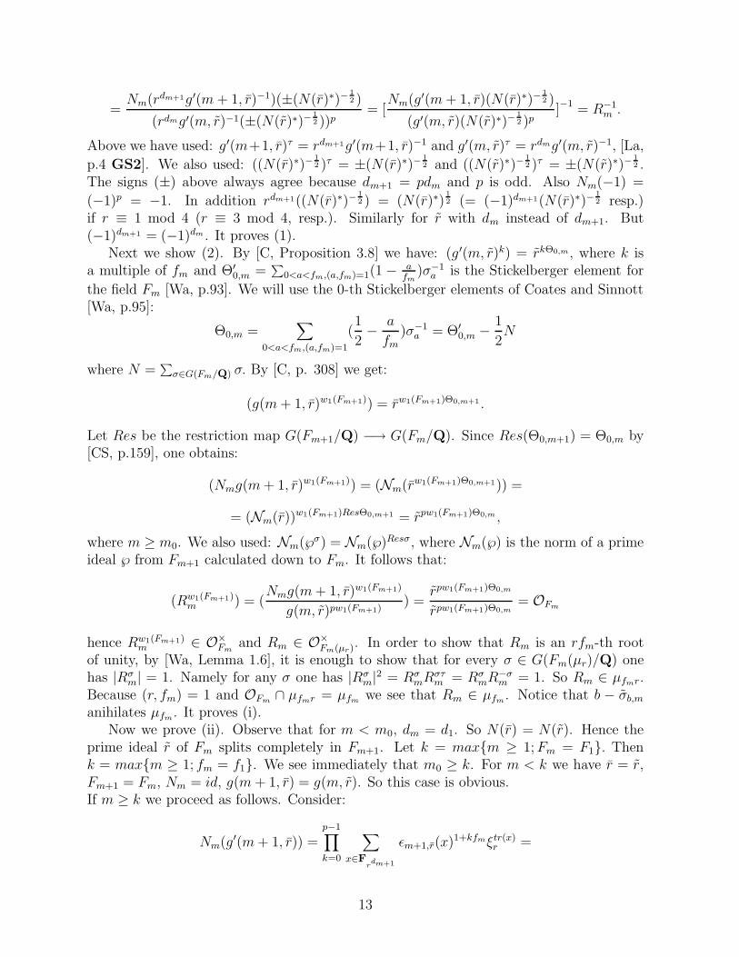
=Nm(rdm+1g′(m + 1, r)−1)(±(N(r)∗)−
12 )
(rdmg′(m, r)−1(±(N(r)∗)−12 ))p
= [Nm(g′(m+ 1, r)(N(r)∗)−
12 )
(g′(m, r)(N(r)∗)−12 )p
]−1 = R−1m .
Above we have used: g′(m+1, r)τ = rdm+1g′(m+1, r)−1 and g′(m, r)τ = rdmg′(m, r)−1, [La,
p.4 GS2]. We also used: ((N(r)∗)−12 )τ = ±(N(r)∗)−
12 and ((N(r)∗)−
12 )τ = ±(N(r)∗)−
12 .
The signs (±) above always agree because dm+1 = pdm and p is odd. Also Nm(−1) =
(−1)p = −1. In addition rdm+1((N(r)∗)−12 ) = (N(r)∗)
12 (= (−1)dm+1(N(r)∗)−
12 resp.)
if r ≡ 1 mod 4 (r ≡ 3 mod 4, resp.). Similarly for r with dm instead of dm+1. But(−1)dm+1 = (−1)dm . It proves (1).
Next we show (2). By [C, Proposition 3.8] we have: (g ′(m, r)k) = rkΘ0,m, where k isa multiple of fm and Θ′0,m =
∑0<a<fm,(a,fm)=1(1 − a
fm)σ−1
a is the Stickelberger element for
the field Fm [Wa, p.93]. We will use the 0-th Stickelberger elements of Coates and Sinnott[Wa, p.95]:
Θ0,m =∑
0<a<fm,(a,fm)=1
(1
2− a
fm)σ−1
a = Θ′0,m − 1
2N
where N =∑σ∈G(Fm/Q) σ. By [C, p. 308] we get:
(g(m+ 1, r)w1(Fm+1)) = rw1(Fm+1)Θ0,m+1 .
Let Res be the restriction map G(Fm+1/Q) −→ G(Fm/Q). Since Res(Θ0,m+1) = Θ0,m by[CS, p.159], one obtains:
(Nmg(m+ 1, r)w1(Fm+1)) = (Nm(rw1(Fm+1)Θ0,m+1)) =
= (Nm(r))w1(Fm+1)ResΘ0,m+1 = rpw1(Fm+1)Θ0,m ,
where m ≥ m0. We also used: Nm(℘σ) = Nm(℘)Resσ, where Nm(℘) is the norm of a primeideal ℘ from Fm+1 calculated down to Fm. It follows that:
(Rw1(Fm+1)m ) = (
Nmg(m+ 1, r)w1(Fm+1)
g(m, r)pw1(Fm+1)) =
rpw1(Fm+1)Θ0,m
rpw1(Fm+1)Θ0,m= OFm
hence Rw1(Fm+1)m ∈ O×Fm
and Rm ∈ O×Fm(µr). In order to show that Rm is an rfm-th rootof unity, by [Wa, Lemma 1.6], it is enough to show that for every σ ∈ G(Fm(µr)/Q) onehas |Rσ
m| = 1. Namely for any σ one has |Rσm|2 = Rσ
mRστm = Rσ
mR−σm = 1. So Rm ∈ µfmr.
Because (r, fm) = 1 and OFm ∩ µfmr = µfm we see that Rm ∈ µfm. Notice that b − σb,manihilates µfm. It proves (i).
Now we prove (ii). Observe that for m < m0, dm = d1. So N(r) = N(r). Hence theprime ideal r of Fm splits completely in Fm+1. Let k = max{m ≥ 1;Fm = F1}. Thenk = max{m ≥ 1; fm = f1}. We see immediately that m0 ≥ k. For m < k we have r = r,Fm+1 = Fm, Nm = id, g(m+ 1, r) = g(m, r). So this case is obvious.If m ≥ k we proceed as follows. Consider:
Nm(g′(m+ 1, r)) =p−1∏
k=0
∑
x∈Frdm+1
εm+1,r(x)1+kfmξtr(x)r =
13
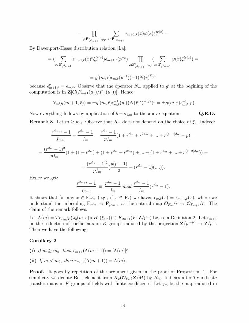
=∏
ϕ:F∗
rdm+1
→µp
∑
x∈Frdm+1
εm+1,r(x)ϕ(x)ξtr(x)r =
By Davenport-Hasse distribution relation [La]:
= (∑
x∈Frdm+1
εm+1,r(x)pξtr(x)r )εm+1,r(p−p)
∏
ϕ:F∗
rdm+1
→µp
(∑
x∈Frdm+1
ϕ(x)ξtr(x)r ) =
= g′(m, r)εm,r(p−1)(−1)N(r)
p−12
because εpm+1,r = εm,r. Observe that the operator Nm applied to g′ at the begining of thecomputation is in Z[G(Fm+1(µr)/Fm(µr))]. Hence
Nm(g(m+ 1, r)) = ±g′(m, r)ε−1m,r(p)((N(r)∗)−1/2)p = ±g(m, r)ε−1
m,r(p)
Now everything follows by application of b− σb,m to the above equation. Q.E.D.
Remark 8. Let m ≥ m0. Observe that Rm does not depend on the choice of ξr. Indeed:
rdm+1 − 1
fm+1
− rdm − 1
fm=rdm − 1
pfm(1 + rdm + r2dm + ... + r(p−1)dm − p) =
=(rdm − 1)2
pfm(1 + (1 + rdm) + (1 + rdm + r2dm) + ...+ (1 + rdm + ...+ r(p−2)dm)) =
=(rdm − 1)2
pfm(p(p− 1)
2+ (rdm − 1)(....)).
Hence we get:rdm+1 − 1
fm+1≡ rdm − 1
fmmod
rdm − 1
fm(rdm − 1).
It shows that for any x ∈ Frdm (e.g., if x ∈ Fr) we have: εm,r(x) = εm+1,r(x), where weunderstand the imbedding Frdm → Frdm+1 as the natural map OFm/r → OFm+1/r. Theclaim of the remark follows.
Let Λ(m) = TrFm/F (λb(m, r) ∗Bn(ξpm)) ∈ K2n+1(F ; Z/pm) be as in Definition 2. Let rm+1
be the reduction of coefficients on K-groups induced by the projection Z/pm+1 → Z/pm.Then we have the following.
Corollary 2
(i) If m ≥ m0, then rm+1(Λ(m + 1)) = [Λ(m)]p.
(ii) If m < m0, then rm+1(Λ(m+ 1)) = Λ(m).
Proof. It goes by repetition of the argument given in the proof of Proposition 1. Forsimplicity we denote Bott element from K2(OFm; Z/M) by Bm. Indicies after Tr indicatetransfer maps in K-groups of fields with finite coefficients. Let jm be the map induced in
14
K-theory by inclusion of fields Fm −→ Fm+1. By Proposition 3(i) and basic properties oftransfer maps given in [So3] we have the following equalities:
rm+1(Λ(m+ 1)) = TrFm+1/F ◦ rm+1(λb(m+ 1, r) ∗Bnm+1) =
= TrFm/F ◦ TrFm+1/Fm(rm+1(λb(m+ 1, r)) ∗ rm+1Bnm+1) =
= TrFm/F ◦ TrFm+1/Fm(rm+1(λb(m+ 1, r)) ∗ jmBnm) =
= TrFm/F (Nmλb(m + 1, r) ∗Bnm) = TrFm/F (λb(m, r)
p ∗Bnm) = Λ(m)p,
in case if m ≥ m0. It proves (i). (ii) follows in the same way. Q.E.D.
4 The Euler system {Λ(L, r); L ∈ S} and K∗(Z)
4.1 Divisible elements in K2n(Q) for n odd.
For an abelian p-torsion group A we denote by div A =⋂k≥1 p
kA the subgroup of divisibleelements. It follows from the localization sequence that K2n+1(F ) does not have nontrivialdivisible elements. On the other hand the group K2n(F ) may have nontrivial divisibleelements cf. [Ba2, Section II]. It follows from the exact sequence:
0 → K2n(O) → K2n(F ) →⊕
ν
K2n−1(kν) → 0
that the group Dn+1(F ) = div [K2n(F )p] is contained in K2n(O)p [loc. cit]. Hence Dn+1(F )is finite. The first author together with M.Kolster proved in [Ba2, Theorem 3] that for nodd, p odd and F totally real one has the following formula for the number of elements ofthe group Dn+1(F ).
|Dn+1(F )| = |wn+1(F )ζF (−n)∏ν|pwn(Fν)
|−1p
Proof of the formula given in [Ba2] relies on “the Main Conjecture” in Iwasawa theoryproven by A.Wiles and also on a result of P.Schneider. In the case when n is odd, p anodd prime and F = Q the formula gives: |Dn+1(Q)| = |wn+1(Q)ζQ(−n)|−1
p which is thenumber of elements in K2n(Z)p predicted by the Quillen-Lichtenbaum conjecture. Hencein this case the conjecture is equivalent to saying that K2n(Z)p is divisible in K2n(Q)p.In this section we are going to investigate the number of divisible elements in K2n(Q)p forn odd using the Euler system of elements Λ(L, r). In Section 5 of the paper we prove someresults concerning Dn+1(F ) for n even.
4.2 Kolyvagin operator and elements δn(L)
In this section F = Q, E = Q(µpm) and M = pm. Let GL = G(E(µL)/E). We denote byw : (Z/p)× → Z×p the Teichmuller character defined by a congruence: w(c0) ≡ c0mod p.Let ∆ = {σc ∈ G(E/Q); c ≡ c0mod p, c ≡ w(c0)modM}. Let DL denote the Kolyvaginoperator [Ru2, p.310].
15
Lemma 2
(i) Λ∗(L, r)DL ∈ K2n+1(E(µL); Z/M)GL where Λ∗(L, r) is the Euler system from Section 3constructed for the base field E.
(ii) Λ(L, r)DL ∈ K2n+1(F (µL); Z/M)GL
(iii) Θ∗n(bL)DL ∈ (Z/M)[G(E(µL)/Q)]GL
(iv) Θn(bL)DL ∈ (Z/M)[G(F (µL)/Q)]GL .
Proof. (i) Proof by induction on number of divisors of L as in [Ru2]. Λ∗(L, r)DL(σl−1) =
Λ∗(L, r)DL/l(l−1−Nl) = i(Λ∗(L/l, r)DL/l(lnFr−1
l−1)) = i(Λ∗(L/l, r)DL/l(Fr
−1l−1)) = 0 because
l ≡ 1 mod M and by induction hypothesis. First step of the induction is obvious.We denote by i the natural map on K-theory induced by the inclusion F (µL/l) ⊂ F (µL).We see that i ◦ Trl = Nl on K-groups.
(iii) By (i) Λ∗(L, r)DL(σl−1) = 0 in K2n+1(E(µL); Z/M). Pick r ≡ 1 mod M . Then byProposition 2:
∂′(Λ∗(L, r)bnLDL(σl−1)) = πr(B
n(ξpm))Θ∗n(bL)DL(σl−1).
By assumption on r the element πr(Bn(ξpm)) has order M. So Θ∗n(bL)DL(σl−1) ≡ 0modM
for each l.(ii) and (iv) are proven in the same way as (i) and (iii). Q.E.D.
Now similarly to K. Rubin we can conclude by Lemma 2(iii) and (iv) that there are elementsδ∗n(L) ∈ (Z/M)[G(E/Q)] and δn(L) ∈ Z/M such that:
Θ∗n(bL)DL ≡ NLδ∗n(L)modM
Θn(bL)DL ≡ NLδn(L)modM.
We can also repeat [Ru2, Lemma 2.1] for E as the base field to get an element δ∗0(L) in(Z/M)[G(E/Q)] such that: Θ∗0(bL)DL ≡ NLδ
∗0(L)modM.
Lemma 3 ResE/Q(δ∗n(L)) = (1 − pn)δn(L)
Proof. Applying ResE(µL)/Q(µL) to the congruence which defines δ∗n(L) we get:
(1 − pn)Θn(bL)DL ≡ NL(ResE/Q(δ∗n(L)))modM.
On the other hand we have:
(1 − pn)Θn(bL)DL ≡ (1 − pn)NL(δn(L))modM.
Lemma 3 follows by comparison of these congruencies. Q.E.D.
Our next objective is to find a relationship between δ∗n(L) and δ∗0(L). Observe that:
Θ∗n(bL) =∑
(a,pmL)=1,1≤a<pmL
∆n+1(a, bL, pmL)σ−1
a .
16
Let us write the elements: DL, NL ∈ Z[G(Q(µL)/Q)] and δ∗n(L), δ∗0(L) ∈ (Z/M)[G(E/Q)]explicitly as follows:
DL =∑
(a2,L)=1,1≤a2<L
da2σ−1a2
NL =∑
(a2,L)=1,1≤a2<L
σ−1a2
δ∗n(L) =∑
(a0,pm)=1,1≤a0<pm
Na0σ−1a0
δ∗0(L) =∑
(a0 ,pm)=1,1≤a0<pm
na0σ−1a0,
where da2 ∈ Z and Na0 , na0 ∈ Z/M are uniquely determined coefficients.
Lemma 4Na0 ≡ an0b
nLna0 modM
Proof. Θ∗n(bL)DL =∑
(a2,L)=1,1≤a2<L
∑(a,pmL)=1,1≤a<pmL ∆n+1(a, bL, p
mL)σ−1a da2σ
−1a2
=
=∑
(a2,L)=1,1≤a2<L
[∑
a↔(a0 ,a1)
∆n+1(a, bL, pmL)da2σ
−1a0σ−1a1
]σ−1a2
=
=∑
(a′,L)=1,1≤a′<L
∑
(a0,pm)=1,1≤a0<pm
[∑
a1a2≡a′modL
∆n+1(a, bL, pmL)da2 ]σ−1
a0σ−1a′ .
In the summation above we replaced a ∈ (Z/pmL)× by (a0, a1) ∈ (Z/pm)×× (Z/L)× usingthe obvious isomorphism: Z/pmL→ Z/pm × Z/L. On the other hand:
NLδ∗n(L) =
∑
(a′,L)=1,1≤a′<L
∑
(a0 ,pm)=1,1≤a0<pm
Na0σ−1a0σ−1a′ .
Hence comparison of the above computations gives:
Na0 ≡∑
a1a2≡a′modL
∆n+1(a, bL, pmL)da2 modM
for all a0 and all a′. In the same way we get:
na0 ≡∑
a1a2≡a′modL
∆1(a, bL, pmL)da2 modM.
In addition, by the Coates-Sinnott congruence [CS, Theorem 1.3. (ii)] we have:
Na0 ≡∑
a1a2≡a′modL
anbnL∆1(a, bL, pmL)da2 ≡ an0b
nLna0 modM
because a ≡ a0modM . Q.E.D.
17
4.3 Elements K(L, r)
Fix r ≡ 1 mod pmL and fix r an ideal of E over r. Choose a prime ideal r in E(µL) lyingover r. We know that λbL(r)DL ∈ (E(µL)×/E(µL)×M)G(E(µL)/E) by Lemma 1 and [Ru2,Lemma 2.1] applied to these elements. By [Ru2, Lemma 2.2] the following map:
(E×/E×M)χ → ((E(µL)×/E(µL)×M)G(E(µL)/E))χ
is an isomorphism for each odd character χ 6= w of ∆. Similarly to [Ru2, Prop. 2.3] definek(L, r) ∈ E× by a congruence: k(L, r) ≡ λbL(r)DLeχ modE(µL)×M . Observe that k(L, r)does not depend on the choice of the prime r over r. Define also K(L, r) ∈ K2n+1(Q; Z/M)by the equality: K(L, r) = TrE/Q(k(L, r) ∗Bn(ξpm)).
Proposition 4
(i) If l 6 |Lr, then [k(L, r)]l = 0.
(ii) [k(L; r)]r = δ∗0(L)eχr
(iii) If l 6 |Lr, then ∂l(K(L, r)) = 0.
(iv)
∂r(K(L, r)bnLγp) =
{(Nr/r(πrB
n(ξpm)))δn(L); if χ = w−n
0; if χ 6= w−n.
Proof. (i) and (ii) are proven similarly to [Ru2, Proposition 2.3]. (iii) follows from (i).To prove (iv) we denote by i the map between Quillen localization sequences induced byimbeddings: Q → Q(µL) and E → E(µL). We also put ∂r, ∂
′′r , ∂
′r to be the boundary
operators in the Quillen localization sequences for Q,Q(µL), E(µL), respectively. One has:
i∂r(K(L, r)bnLγp) = ∂′′r i(K(L, r)b
nLγp) =
= ∂′′r (TrE(µL)/Q(µL) ◦ i((k(L, r) ∗Bn(ξpm))bnLγp)) = N ′[∂′r(λbL(r)DLeχ ∗Bn(ξpm))b
nLγp] =
= (N ′(πrBn(ξpm)))Θn(bL)DLeχwn = (N ′(πrB
n(ξpm)))NLδn(L)eχwn =
= i(Nr/r(πrBn(ξpm))δn(L)eχwn ).
The second equality above holds because i ◦ TrE/Q = TrE(µL)/Q(µL) ◦ i.But i : K2n(Fr; Z/M) → ⊕℘|rK2n(k℘; Z/M) (induced by Q → Q(µL)) is an imbedding andResE(µL)/Q(µL)(eχwn) = 0 if χwn 6= 1 and ResE(µL)/Q(µL)(eχwn) = 1 if χwn = 1. So (iv)follows. Q.E.D.
Next proposition follows easily from Proposition 3 and Corollary 2. Recall the number m0
from Proposition 3.
Proposition 5 Let K(m) (K(m − 1)) denote the element K(L, r) (K(L, r)) defined forthe field Q(µpmL) (Q(µpm−1L), resp). Here r denotes the prime ideal in Q(µpm−1L) below r.
(i) If m− 1 ≥ m0, then rm(K(m)) = [K(m− 1)]p.
18
(ii) If m− 1 < m0, then rm(K(m)) = K(m− 1).
Definition 4 Let ℘|l be a prime ideal of E. Define
ϕ℘ : {x ∈ E×/E×M ; [x]l = 0} → (Z/M)[G(E/Q)]
ϕ℘(x) ≡∑
σ∈G(E/Q)
v℘σ(x)σmodM,
where x is a lifting of x to E× prime to l.
We have the following analog for E/Q of [Ru2, Theorem 2.4].
Theorem 1 Let L ∈ S and let r and r′ be primes of E over distinct rational primesr ≡ r′ ≡ 1 mod M2L. Let A(L) be the p part of the ideal class group of E(µL) and let rand r′ be ideals of E(µL) above r and r′ respectively whose projections into A(L)χ are thesame. Then: ϕr(k(L, r′)) ≡ δ∗0(Lr)eχmod δ
∗0(L)eχ(Z/M)[G(E/Q)].
Proof. Observe that we have:
k(L, r) = λbL(r)DLeχ = G(εL,r;ψ)(bL−σbL)DLeχ = G(ε−1
L,r;ψ)(σbL−bL)DLeχ ,
where we have used the standard notation for the Gauss sums: G(εL,a¯rr;ψ) = g(L, r, ξr)
[cf. Definition 3] and ψ(x) = ξtrxr in order to indicate that g depends on εL,r. It follows thatwe are able to use proof of Theorem 2.4. of [Ru2] if we adjust it to our situation. Below isa list of necessary adjustments.1) Lemma 2.5 holds without any change in our case.2) Corollary 2.6 holds if one puts: s′(L, r) =
∑a∈Z/ML× vr(− 1
(at)!)τ−1a modM, where
t = r−1ML
for r ≡ 1modM 2L, Θ′(L, r, χ) = eχ(σbL − bL)s′(L, r), and put also:
Θ(L, χ) = eχΘ(L) =1
ML(σbL − bL)s(L).
3) In Proposition 2.7 we need to take E instead of F, r as above, r a prime of E above r,and π ∈ E×. The conclusion of the proposition says in our case that:
ϕr(k(L, r)
πδ∗0(L)eχ
) = δ∗0(Lr)eχ,
where ϕr is as in Definition 4.4) Proposition 2.8 reformulates as follows.
Let L ∈ S, r, r′ be primes of E lying above distinct rational primes r and r′ such that
r ≡ r′ ≡ 1modM. Let A(L) be the p-part of the ideal class group of E(µL) and let us
suppose that r and r′ are prime ideals of E(µL) above r and r′, respectively, such that they
map to the same class in A(L)χ. Then we have:
k(L, r′)/k(L, r) ∈ E×δ∗0 (L)eχE×M
E×M.
19
Proof of Theorem 1 now goes in the same way as the proof of Theorem 2.4 in [Ru2]. Q.E.D.
Let OE be the ring of integers in E, and let ℘ be a prime ideal in OE with a residue fieldk℘. Let π℘ : OE → k℘ be the reduction map. As usual, π℘ denotes also the map inducedon K-theory. Observe that the following diagram commutes.
K2n+1(OE[1/Lr]; Z/M)⊕℘|lπ℘−→ ⊕
℘|lK2n+1(k℘; Z/M)
↓ Tr ↓ ⊕N℘/l
K2n+1(Z[1/Lr]; Z/M)πl→ K2n+1(Fl; Z/M)
Diagram 6
Notice that K(L, r) ∈ K2n+1(Z[1/Lr]; Z/M). Take l 6 |Lr. Let gl be a generator of F×l . Forany prime ideal ℘ of E such that ℘|l define v℘ as in [Ru2] by the congruence:
k(L, r) ≡ gv℘(k(L,r))l mod ℘.
Theorem 2 Let (l, Lr) = 1 and let l ≡ 1modM 2L. Then there is an integer k such that:πl(K(L, r)b
nLγp) = N℘/l(gl ∗ π℘(Bn(ξpm)))δn(Ll)+δn(L)k.
Proof. πl(K(L, r)bnLγp) = (πl(K(L, r)))b
nLγp = (
∏℘|lN℘/l(π℘(k(L, r) ∗Bn(ξpm))))b
nLγp =
= (∏
1≤a<pm,(a,p)=1
N℘σ−1
a /l(gv
℘σ−1a
(k(L,r))
l ∗ π℘σ−1
a(Bn(ξpm))))b
nLγp =
= (∏
1≤a<pm,(a,p)=1
N℘σ−1
a /l((gl ∗ π℘σ−1
a(Bn(ξpm)a
nσ−1a ))
v℘σ
−1a
(k(L,r))))b
nLγp =
= (∏
1≤a<pm,(a,p)=1
(N℘/l(gl ∗ π℘(Bn(ξpm)))anv
℘σ−1a
(k(L,r))σ−1a
)bnLγp =
= ((N℘/l(gl ∗ π℘(Bn(ξpm))))
∑1≤a<pm,(a,p)=1
anv℘σ−1
a(k(L,r))σ−1
a
)bnLγp
= ((N℘/l(gl ∗ π℘(Bn(ξpm))))
∑1≤a<pm,(a,p)=1
anv℘σ−1
a(k(L,r))
)bnLγp .
Theorem 2 follows from Lemma 3 and Lemma 5 which is stated below. Observe that:(1 − pn)ResE/Q(γp) ≡ 1modM . From now on we assume that χ = w−n and that χ 6= w,i.e., n 6≡ −1mod (p− 1).
Lemma 5
∑
1≤a<pm,(a,p)=1
bnLanv
℘σ−1a
(k(L, r)) ≡ ResE/Q(δ∗n(Ll))modResE/Q(δ∗n(L))(Z/M)
20
Proof. To simplify this proof we will write ≡ instead of ≡ mod M . We work with thecharacter χ = w−n. Denote
δ∗0(Ll) =∑
1≤a<pm,(a,p)=1
naσ−1a ,
δ∗0(L) =∑
1≤a<pm,(a,p)=1
maσ−1a .
By Theorem 1 from previous section we have: ϕ℘(k(L, r)) ≡ δ∗0(Ll)eχ + δ∗0(L)eχη, whereη ∈ (Z/M)[G(E/Q)]. Let us write η =
∑1≤a<pm,(a,p)=1 laσ
−1a .
δ∗0(Ll)eχ = (∑
1≤a′<pm,(a′,p)=1
na′σ−1a′ )(
1
p− 1
∑
σc∈∆
w−n(σc)σ−1c ) =
=1
p− 1
∑
1≤a<pm,(a,p)=1
(∑
a′c≡a
na′c−n)σ−1
a .
In the same way:
δ∗0(L)ηeχ = (∑
1≤a0<pm,(a0,p)=1
ma0σ−1a0
)(∑
1≤a1<pm,(a1,p)=1
la1σ−1a1
)(1
p− 1
∑
σc∈∆
w−n(σc)σ−1c ) =
=1
p− 1
∑
1≤a<pm,(a,p)=1
[∑
a′c≡a
(∑
a0a1≡a′ma0 la1)c−n]σ−1
a .
So by Theorem 1: ∑
1≤a<pm,(a,p)=1
anv℘σ−1
a(k(L, r)) ≡
≡ 1
p− 1
∑
1≤a<pm,(a,p)=1
(∑
a′c≡a
a′nna′) +1
p− 1
∑
1≤a<pm,(a,p)=1
∑
a′c≡a
(∑
a0a1≡a′a′nma0 la1) ≡
≡∑
1≤a<pm,(a,p)=1
anna +∑
1≤a<pm,(a,p)=1
∑
a0a1≡a
an0ma0an1 la1 ≡
≡∑
1≤a<pm,(a,p)=1
anna + (∑
1≤a0<pm,(a0,p)=1
an0ma0)(∑
1≤a1<pm,(a1,p)=1
an1 la1).
Hence multiplying by bnL and using Lemma 4 we get Lemma 5. Q.E.D
4.4 Etale cohomology and Chebotarev density theorem
In this section we collect some results on the structure of etale cohomology groups andelements K(L, r) which are crucial for applications of the Euler system of elements Λ toK-theory of the rationals, presented in the next section. From now on we work in etaleK-theory and etale cohomology. Let KM denote the element of
Ket2n+1(Z[
1
Lpr]; Z/M) ∼= H1
et(Z[1
Lpr]; Z/M(n+ 1))
21
obtained from K(L, r) ∈ K2n+1(Z[ 1Lpr
]; Z/M) via the map of Dwyer and Friedlander cf.
[DF]. Observe that all properties of K(L, r) which we have proved until now imply similarstatements for elements KM . It follows immediately from functorial properties of the mapof Dwyer and Friedlander. We assume that r ≡ 1 modM 2L.
Lemma 6 Let S be a finite set of prime numbers which contains p, r and all prime divisorsof L. Assume that KM ∈ H1
et(ZS,Z/M(n + 1)) is nonzero and that p does not dividewn+1(Q). Then in H1
et(ZS,Z/M(n + 1)) there is a free Z/M-module which contains KM .
Proof. Let M1 be a power of p such that M |M1. Consider a commutative diagram.
H1et(ZS; Z/M1(n+ 1)) → H2
cont(ZS ; Zp(n+ 1))[M1]
↓ red ↓H1et(ZS; Z/M(n + 1)) → H2
cont(ZS; Zp(n+ 1))[M ]
Diagram 7
In the diagram the right vertical map is multiplication by M1
Mand the left vertical map
comes from reduction of coefficients. Horizontal maps in the diagram come from Bocksteinsequence in continous cohomology on SpecZS. Let t be the order of KM . We chooseM1 = M2
t. Since M ≤ M1 ≤ M2, Proposition 5(ii) implies that red(KM1) = KM . Recall
that the group H1et(ZS ; Zp(n + 1)) has |wn+1(Q)|−1
p elements, cf. [So3]. By assumption pdoes not divide the number wn+1(Q). Hence the lower horizontal map in Diagram 7 isan isomorphism. Let x be the image of KM1 under the upper horizontal map and let y
denote the image of KM under the lower map of the diagram. We have y = xM1M = x
Mt . It
implies equality: 1 = yt = xM . Hence x ∈ H2cont(ZS; Zp(n + 1))[M ]. By surjectivity of the
lower horizontal map we can pick T from H1et(ZS ; Z/M(n + 1)) which maps onto x. Then
TMt maps onto y and injectivity of the lower horizontal map implies that KM = T
Mt . KM
is nonzero by assumption, hence T is nonzero, too. It follows that KM belongs to a freeZ/M -module generated by T which is contained in H1
et(ZS; Z/M(n + 1)). Q.E.D.
In the sequel we keep assumptions of Lemma 6, i.e., we assume that p 6 |wn+1(Q) and thatKM 6= 0. Let ps be the largest power of p such that KM = psy, for some y from the groupH1et(ZS; Z/M(n + 1)). By Lemma 6 the order of KM equals M
ps . Let E = Q(µM) and let
OE, (OE,S , respectively) be the ring of integers (S-integers) in E. From now on we chooseS to be a finite set of prime numbers which contains: p, r, all prime divisors of L, and inaddition has a property that PicOE,S vanishes. For a prime number l 6∈ S, and a primeideal λ from OE,S which lies above l, we have the following commutative diagram whosehorizontal arrows are induced by reduction maps.
H1et(ZS; Z/M(n + 1)) → H1
et(kl; Z/M(n + 1))
↓ ↓H1et(OE,S; Z/M(n + 1)) → H1
et(kλ; Z/M(n+ 1))
Diagram 8
We want to prove that the left, vertical map in the diagram is injective under our assump-tions. The Hochschild-Serre spectral sequence
Er,s2 = Hr(G(E/Q);Hs
et(OE,S; Z/M(n+ 1))) =⇒ Hr+set (ZS; Z/M(n + 1))
22
gives the following exact sequence of low terms.
0 → H1(G(E/Q); Z/M(n+ 1)) → H1et(ZS; Z/M(n + 1)) → H1
et(OE,S; Z/M(n + 1))G(E/Q)
On the other hand, by Herbrand quotient we have:
| H1(G(E/Q); Z/M(n+ 1)) |= | H0Tate(G(E/Q); Z/M(n + 1)) | .
In addition: | H0Tate(G(E/Q); Z/M(n + 1)) | ≤ | H0(G(E/Q); Z/M(n+ 1)) |=
= | H0(G(Q∞/Q); Z/M(n + 1)) | ≤ | H0(G(Q∞/Q); Qp/Zp(n+ 1)) |= | wn+1(Q) |−1p .
The last equality follows from [So3]. Since by assumption p does not divide wn+1(Q), itfollows that H1(G(E/Q); Z/M(n + 1)) = 0 and the left map in Diagram 8 is injective.The exact sequence of sheaves for etale cohomology on SpecOE,S:
0 → Z/M(1) → GmM→ Gm → 1
and assumption PicOE,S = 0 show that one has an isomorphism:
O×E,S/O×ME,S ∼−→ H1et(OE,S; Z/M(1)).
Tensoring with Z/M(n) gives an isomorphism:
O×E,S/O×ME,S ⊗ Z/M(n)∼−→ H1
et(OE,S; Z/M(n + 1)).
In a similar way one gets an isomorphism:
k×λ /k×Mλ ⊗ Z/M(n)
∼−→ H1et(kλ; Z/M(n + 1)).
Under the last two isomorphisms the bottom horizontal map in Diagram 8 identifies easilywith the map:
O×E,S/O×ME,S ⊗ Z/M(n) −→ k×λ /k×Mλ ⊗ Z/M(n)
which is induced by reduction at λ. Let ξ be a generator of Z/M(1). Then ξ⊗n is a generatorof Z/M(n). Let β⊗ξ⊗n ∈ O×E,S/O×ME,S ⊗Z/M(n) be the image of KM under the left verticalmap from Diagram 8. We consider β to be the image of an element (also denoted by β)from O×E,S. It follows by Lemma 6 that β ⊗ ξ⊗n is of order M
ps . We want to prove that
the image of β ⊗ ξ⊗n under the lower horizontal map in Diagram 8 has also order Mps for
some choices of prime ideals λ. To choose λ′s with this property we will use a theorem ofK.Rubin [Ru2, Theorem 3.1] which is based on Chebotarev density theorem. Observe thatfor our reason it is enough to consider the map O×E,S/O×ME,S −→ k×λ /k
×Mλ induced by the
reduction. First we need two lemmas.
Lemma 7 Let α ∈ O×E,S/O×ME,S and let t be the maximal power of p such that α is in
O×tE,S/O×ME,S . Then t is also the largest power of p such that α ∈ E×t/E×M . In addition, the
order of α is Mt.
23
Proof. Let t1 be the maximal power of p such that α ∈ E×t1/E×M . Then α = yt1zM for
some y and z from E. Hence α = (yzMt1 )t1 and obviously yz
Mt1 ∈ O×E,S. So t1 | t by the
definition of t. On the other hand O×E,S ⊆ E×, hence t1 | t by definition of t1.
Let now t1 be the order of α in O×E,S/O×ME,S . Then αt1 = zM , for some z ∈ O×E,S. Hence
α = zMt1 η, where ηt1 = 1 and η ∈ E. Since all Mth roots of unity are in E, there is ξ ∈ E
such that η = ξMt1 and α = (zξ)
Mt1 . Obviously zξ ∈ O×E,S. It follows by the definition of t
that Mt1
| t hence Mt| t1. On the other hand, α
Mt1 = 1 because α ∈ O×E,S/O×ME,S , hence t1
divides Mt
by the definition of t1. Q.E.D.
We apply Lemma 7 to α = β where β is the element of O×E,S/O×ME,S associated to KM inour previous discussion. It follows that t = ps, i.e., t - the largest power of p such thatβ ∈ O×tE,S/O×ME,S equals ps - the largest power of p which divides KM in H1
et(ZS; Z/M(n+1)).We omit a proof of the next lemma which follows by an argument similar to that afterDiagram 8.
Lemma 8 If KM is nonzero, then the highest powers of p which divide KM in the groupsH1et(ZS; Z/M(n + 1)) and H1
et(Q; Z/M(n + 1)) are the same.
Theorem 3 Let α ∈ O×E,S/O×ME,S , ℘ ∈ Pic (OE(µL)), and let t be the maximal power of p
such that α is in O×tE,S/O×ME,S . There exist infinitely many prime ideals λ in OE such thatthere is a prime ideal in OE(µL) lying above λ, which is in the ideal class ℘. If l is the primenumber below λ, then l ≡ 1modM 2L. The image of α in k×λ /k
×Mλ has order M
t.
Proof. [Ru2, Theorem 3.1.]
Let πl be the map induced on etale K-theory by the reduction ZS → kl. Pick λ and l as inTheorem 3. Let gl∗πλ(Bn(ξpm)) be the generator ofKet
2n+1(kλ; Z/M) ∼= H1et(kλ; Z/M(n+1)).
The following proposition will be crucial in the next section. It is an immediate corollaryof what we have proved in this section.
Proposition 6 If KM is nonzero and p does not divide wn+1(Q), then for prime numbersl from Theorem 3 we have: πl(KM) = [gl ∗ πλ(Bn(ξpm))]νt for some ν ∈ (Z/M)×, where tis the largest power of p dividing KM in the group H1
et(Q; Z/M(n + 1)).
We finish this section with a result which may be of some independend interest. LetY be a submodule of O×E,S/O×ME,S which consists of all y such that any σa ∈ G(E/Q) actsat y raising it to the a−nth power. It follows easily from the definition that Y equalsH1et(OE,S; Z/M(n + 1))G(E/Q). Note that by construction and Lemma 6 KM ∈ Y.
Proposition 7 If the element KM is nonzero, then the module Y contains a free Z/M-submodule.
Proof. It follows by Lemma 6 and the HS spectral sequence argument after Diagram 8.Q.E.D.
24
4.5 An application of the Euler system
In this section we show how the elements K(L, r) may be used in K-theory of Q. Weprove in Corollary 3 that the number of divisible elements in p-torsion part of the groupK2n(Q) does not exceed the maximal power of p which divides the number wn+1(Q)ζQ(−n)provided that p does not divide wn+1(Q). Note that Theorem 3 of [Ba2] implies equalityof the two above mentioned powers of p. Though weaker, Corollary 3 has an advantageover [Ba2, Theorem 3], since it does not use “the Main Conjecture” in Iwasawa theory.Its proof relies instead on the properties of elements K(L, r) which we have obtained untilnow. Our argument parallels Rubin’s proof of the Main Conjecture for the odd part of theideal class group of Q(µp) [Ru2, Section 4].
Let us introduce notation which will be used in the sequel. As in the previous section, pis an odd prime not dividing wn+1(Q). M is a power of p which will be specified by Lemma 9and Theorem 4 below. L =
∏l is a square-free integer whose prime divisors l are congruent
to 1 modulo M. We keep L fixed until Corollary 3. For simplicity, we denote Dn+1(Q) by A.Let ψ:
⊕l 6=pK
et2n(Fl; Z/M) → A be a map from the localization sequence [Ba2, Diagram 2.4]
and let vl denote ψ(ξ⊗npm ), where ξ⊗npm is a generator of Ket2n(Fl; Z/M) ∼= H0
et(Fl; Z/M(n)).Let B denote a subgroup of A generated by the vl’s such that l | L. Finally, we fix (againuntil Corollary 3) a generator u of a cyclic summand of the quotient group A/B. Next wewant to choose primes r and r in order to construct elements K(L, r).
Lemma 9 For M big enough, there is an exact sequence:
Ket2n+1(Q; Z/M)
∂→⊕
l 6=pKet
2n(Fl; Z/M)ψ→ A→ 0.
The map ψ restricted to⊕
l≡1modM2LKet2n(Fl; Z/M) has still image A.
Proof. Lemma follows by [Ba2, p.291] and [Ku, Proof of Prop. 1.1]. Q.E.D.
Let r be a prime number such that r ≡ 1modM 2L and that the image of vr in A/B underprojection map generates the same cyclic summand as u does. It can be chosen by Lemma9. Let r be a fixed prime ideal in E(µL) lying above r. The following theorem is an analogueof Theorem 4.1 of [Ru2]. Let dn(L) be the largest power of p which divides number δn(L)defined in Section 4.2.
Theorem 4 Let M be so big that it is divisible by |A|dn(1)p. In addition, assume that
dn(L) | dn(1). Then there is a prime number l such that: l ≡ 1modM 2L and dn(L)dn(Ll)
u = 0
in the group A/B.
Proof. It follows by assumptions that dn(L)p divides M. Hence by Proposition 4, ∂r(KbnLγp
M )is nonzero and consequently KM 6= 0. Proposition 4 implies also that:
∂(KbnLγp
M ) = ∂r(KbnLγp
M ) +∑
l|L
∂l(KbnLγp
M ) = (Nr/r(πr(Bn(ξpm))))δn(L) +
∑
l|L
∂l(KbnLγp
M ).
Let t be, as in the previous section, the highest power of p which divides KM in the groupH1et(Q; Z/M(n+ 1)). It follows from the last equalities that t divides dn(L). But dn(L) |M
25
by assumption, hence t divides M. To proceed with the proof, apply the map ψ to bothsides of the equalities, divide the result by t, and finally project down to A/B. We obtainin this way the following equality.
0 = ψ(∂(KbnLγp
M )) =dn(L)
tu
Since u 6= 0, the number dn(L) is divisible by pt. To conclude the proof it remains to finda prime l which is congruent to 1 modulo M 2L and such that t = dn(Ll). By Theorem 3and Proposition 6 there is an l such that l ≡ 1modM 2L and for which
πl(KbnLγp
M ) = [gl ∗ πλ(Bn(ξpm))]ν1t,
for some ν1 ∈ (Z/M)×. On the other hand Theorem 2 implies:
πl(KbnLγp
M ) = [gl ∗ πλ(Bn(ξpm))]δn(Ll)+kδn(L)
for some integer k. (Recall that, by assumption, p does not divide bL.) Comparing the righthand sides of the last two equalities, we obtain that t ≡ |δn(Ll) + kδn(L)|−1
p modM. Sincept | dn(L), it follows easily that t = dn(Ll) for the prime l. Q.E.D.
Corollary 3 The number of elements of the group A = Dn+1(Q) divides the number|wn+1(Q)ζQ(−n)|−1
p for primes p relatively prime to wn+1(Q), where n is an odd integerand n 6≡ −1mod (p− 1).
Proof. Let u1, u2, ... , ua be generators of cyclic summands, one generator for a summand,in the decomposition of A/B into cyclic groups. Let ci denote the order of the image ofui in the quotient group A/(B, u1, u2, ..., ui−1). We have obviously: |A/B| =
∏ci. Assume
that M is as in Theorem 4 and that dn(L) divides dn(1). Applying Theorem 4 inductively,we obtain prime numbers l1, l2, ..., la which have the following properties.
1. li ≡ 1modM2L
2. the number dn(Li) divides dn(Li−1), where we put L0 = L, and Li = L∏j≤i lj.
In addition we have equality dn(Li−1)dn(Li)
ui = 0, in the group A/(B, u1, u2, ..., ui−1) fori = 1, 2, ..., a.
It follows that |A/B| =∏ci divides
∏ dn(Li−1)dn(Li)
hence also dn(L). Putting L = 1 in the above
implies that the number of elements in A = Dn+1(Q) divides the number dn(1). Recallthat dn(1) = |δn(1)|−1
p = |(bn+11 − 1)ζQ(−n)|−1
p and (b1, pwn+1(Q)) = 1, by assumptionon numbers bL. Taking minimum over numbers b1 gives the final claim by [C, Lemma 2.3].Q.E.D.
5 A class number formula for higher K-groups
5.1 Divisible elements in K2n(F ) for n even
In this section we prove an analogue of a class number formula of Kummer for higher K-groups of number fields. Let n be a positive integer and let F be a totally real, abelian
26
number field with ring of integers OF . We assume for technical reasons that p does notdivide the conductor of F. In [So1, 3.1.2] Soule defined a subgroup of cyclotomic elementsin K2n+1(OF ) ⊗ Zp. The subgroup is generated by elements which are obtained fromcyclotomic units of OF in a similar way as the elements Λ(L) were obtained in Section2 from α(L). We denote Soule’s group of cyclotomic elements by C2n+1 = C2n+1(F ). Itfollows by [So1, Theorem 1] and [So2, Remark 6.4] that the index of C2n+1 inK2n+1(OF )⊗Zp
is finite. Let Cet2n+1 = Cet
2n+1(F ) be the image of C2n+1 by the Dwyer-Friedlander map:
ρ : K2n+1(OF ) ⊗ Zp −→ Ket2n+1(OF [
1
p]).
Since ρ is surjective [loc.cit., Theorem 8.7], it follows that the index of Cet2n+1 in the group
Ket2n+1(OF [1
p]) is finite. Let Dn+1(F ) be the group of divisible elements in K2n(F )p from
Section 4.1. In the case when n is even we have the following formula for the number ofelements of Dn+1(F ). It is the main result of the section.
Theorem 5 Let p and F be as above and let n be even. Then
|Dn+1(F )| = [Ket2n+1(OF [ 1
p]);Cet
2n+1]
Before presenting a proof of the theorem three remarks are in order.
Remark 9. We think that the formula is an anologue for K-groups of the number fieldF of the classical Kummer’s formula h+ = [E; E ], [La, Theorem 5.1, p.85] for the secondfactor of class number of the cyclotomic field Q(ξpk). Here E and E are units and cyclotomicunits in the ring Z[ξpk]. In this analogy Dn+1(F ) replaces the ideal class group. More onthe analogy may be found in [Ba2, p.292].
Remark 10. If the map ρ is an isomorphism (as was conjectured by Dwyer and Friedlan-der), then a similar formula holds for K2n+1(OF ) ⊗ Zp and C2n+1.
Remark 11. Note that in the case of F = Q one can prove that |Dn+1(Q)| divides[Ket
2n+1(Z[1p]);Cet
2n+1] in an elementary way, using the Euler system of cyclotomic units [Ku,
Section 5]. It is so because Dn+1(Q) ∼= H2et(Z[ 1
p]; Zp(n + 1)), [cf. proof of Prop. 8 below]
and the statement follows now from [Ku, Prop. 5.1].
Our proof of Theorem 5 generalizes an argument of Bloch and Kato who showed that ifF is Q, then |Ket
2n(Z[1p])| = [Ket
2n+1(Z[ 1p];Cet
2n+1]. The proof given below uses ”the MainConjecture” in Iwasawa theory.
Proof of Theotem 5. Consider the following diagram [BK, p.387].
27
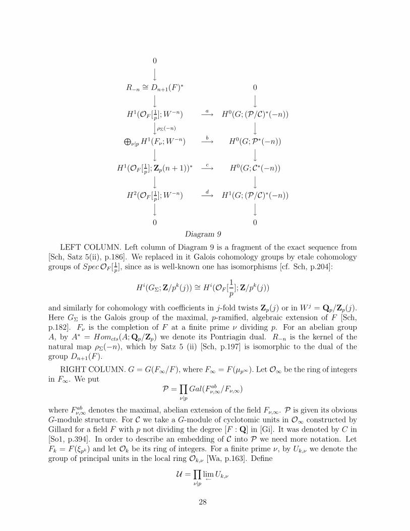
0y
R−n ∼= Dn+1(F )∗ 0y
y
H1(OF [1p];W−n)
a−→ H0(G; (P/C)∗(−n))yρΣ(−n)
y⊕
ν|pH1(Fν;W
−n)b−→ H0(G;P∗(−n))
yy
H1(OF [1p]; Zp(n+ 1))∗
c−→ H0(G; C∗(−n))y
y
H2(OF [1p];W−n)
d−→ H1(G; (P/C)∗(−n))y
y
0 0
Diagram 9
LEFT COLUMN. Left column of Diagram 9 is a fragment of the exact sequence from[Sch, Satz 5(ii), p.186]. We replaced in it Galois cohomology groups by etale cohomologygroups of SpecOF [ 1
p], since as is well-known one has isomorphisms [cf. Sch, p.204]:
H i(GΣ; Z/pk(j)) ∼= H i(OF [1
p]; Z/pk(j))
and similarly for cohomology with coefficients in j-fold twists Zp(j) or in W j = Qp/Zp(j).Here GΣ is the Galois group of the maximal, p-ramified, algebraic extension of F [Sch,p.182]. Fν is the completion of F at a finite prime ν dividing p. For an abelian groupA, by A∗ = Homcts(A; Qp/Zp) we denote its Pontriagin dual. R−n is the kernel of thenatural map ρΣ(−n), which by Satz 5 (ii) [Sch, p.197] is isomorphic to the dual of thegroup Dn+1(F ).
RIGHT COLUMN. G = G(F∞/F ), where F∞ = F (µp∞). Let O∞ be the ring of integersin F∞. We put
P =∏
ν|p
Gal(F abν,∞/Fν,∞)
where F abν,∞ denotes the maximal, abelian extension of the field Fν,∞. P is given its obvious
G-module structure. For C we take a G-module of cyclotomic units in O∞ constructed byGillard for a field F with p not dividing the degree [F : Q] in [Gi]. It was denoted by C in[So1, p.394]. In order to describe an embedding of C into P we need more notation. LetFk = F (ξpk) and let Ok be its ring of integers. For a finite prime ν, by Uk,ν we denote thegroup of principal units in the local ring Ok,ν [Wa, p.163]. Define
U =∏
ν|p
lim←Uk,ν
28
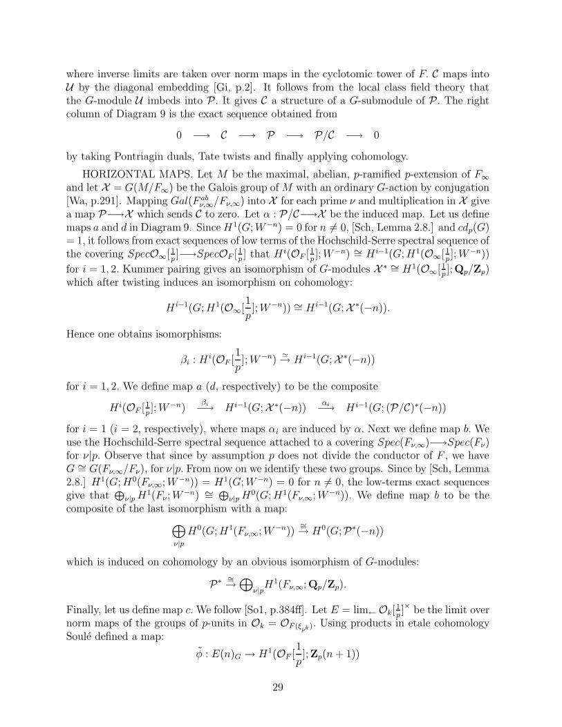
where inverse limits are taken over norm maps in the cyclotomic tower of F. C maps intoU by the diagonal embedding [Gi, p.2]. It follows from the local class field theory thatthe G-module U imbeds into P. It gives C a structure of a G-submodule of P. The rightcolumn of Diagram 9 is the exact sequence obtained from
0 −→ C −→ P −→ P/C −→ 0
by taking Pontriagin duals, Tate twists and finally applying cohomology.
HORIZONTAL MAPS. Let M be the maximal, abelian, p-ramified p-extension of F∞and let X = G(M/F∞) be the Galois group of M with an ordinary G-action by conjugation[Wa, p.291]. Mapping Gal(F ab
ν,∞/Fν,∞) into X for each prime ν and multiplication in X givea map P−→X which sends C to zero. Let α : P/C−→X be the induced map. Let us definemaps a and d in Diagram 9. Since H1(G;W−n) = 0 for n 6= 0, [Sch, Lemma 2.8.] and cdp(G)= 1, it follows from exact sequences of low terms of the Hochschild-Serre spectral sequence ofthe covering SpecO∞[1
p]−→SpecOF [1
p] that H i(OF [1
p];W−n) ∼= H i−1(G;H1(O∞[1
p];W−n))
for i = 1, 2. Kummer pairing gives an isomorphism of G-modules X ∗ ∼= H1(O∞[1p]; Qp/Zp)
which after twisting induces an isomorphism on cohomology:
H i−1(G;H1(O∞[1
p];W−n)) ∼= H i−1(G;X ∗(−n)).
Hence one obtains isomorphisms:
βi : H i(OF [1
p];W−n)
'→ H i−1(G;X ∗(−n))
for i = 1, 2. We define map a (d, respectively) to be the composite
H i(OF [1p];W−n)
βi−→ H i−1(G;X ∗(−n))αi−→ H i−1(G; (P/C)∗(−n))
for i = 1 (i = 2, respectively), where maps αi are induced by α. Next we define map b. Weuse the Hochschild-Serre spectral sequence attached to a covering Spec(Fν,∞)−→Spec(Fν)for ν|p. Observe that since by assumption p does not divide the conductor of F , we haveG ∼= G(Fν,∞/Fν), for ν|p. From now on we identify these two groups. Since by [Sch, Lemma2.8.] H1(G;H0(Fν,∞;W−n)) = H1(G;W−n) = 0 for n 6= 0, the low-terms exact sequencesgive that
⊕ν|pH
1(Fν ;W−n) ∼= ⊕
ν|pH0(G;H1(Fν,∞;W−n)). We define map b to be the
composite of the last isomorphism with a map:⊕
ν|p
H0(G;H1(Fν,∞;W−n))∼=→ H0(G;P∗(−n))
which is induced on cohomology by an obvious isomorphism of G-modules:
P∗ ∼=→⊕
ν|pH1(Fν,∞; Qp/Zp).
Finally, let us define map c. We follow [So1, p.384ff]. Let E = lim←Ok[1p]× be the limit over
norm maps of the groups of p-units in Ok = OF (ξpk ). Using products in etale cohomology
Soule defined a map:
φ : E(n)G → H1(OF [1
p]; Zp(n+ 1))
29
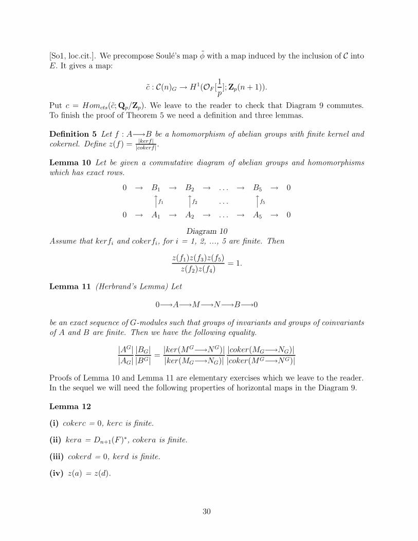
[So1, loc.cit.]. We precompose Soule’s map φ with a map induced by the inclusion of C intoE. It gives a map:
c : C(n)G → H1(OF [1
p]; Zp(n+ 1)).
Put c = Homcts(c; Qp/Zp). We leave to the reader to check that Diagram 9 commutes.To finish the proof of Theorem 5 we need a definition and three lemmas.
Definition 5 Let f : A−→B be a homomorphism of abelian groups with finite kernel andcokernel. Define z(f) = |kerf |
|cokerf |.
Lemma 10 Let be given a commutative diagram of abelian groups and homomorphismswhich has exact rows.
0 → B1 → B2 → . . . → B5 → 0xf1
xf2 . . .xf5
0 → A1 → A2 → . . . → A5 → 0
Diagram 10
Assume that kerfi and cokerfi, for i = 1, 2, ..., 5 are finite. Then
z(f1)z(f3)z(f5)
z(f2)z(f4)= 1.
Lemma 11 (Herbrand’s Lemma) Let
0−→A−→M−→N−→B−→0
be an exact sequence of G-modules such that groups of invariants and groups of coinvariantsof A and B are finite. Then we have the following equality.
|AG||AG|
|BG||BG| =
|ker(MG−→NG)||ker(MG−→NG)|
|coker(MG−→NG)||coker(MG−→NG)|
Proofs of Lemma 10 and Lemma 11 are elementary exercises which we leave to the reader.In the sequel we will need the following properties of horizontal maps in the Diagram 9.
Lemma 12
(i) cokerc = 0, kerc is finite.
(ii) kera = Dn+1(F )∗, cokera is finite.
(iii) cokerd = 0, kerd is finite.
(iv) z(a) = z(d).
30
Proof. (i) kerc and cokerc are finite groups because φ is a rational isomorphism of finitelygenerated abelian groups, [So1,p.384] and C(n)G is a subgroup of finite index in E(n)G,[So2, Theoreme 3 and Remarque 6.4.]. Hence, kerc = (cokerc)∗ and cokerc = (kerc)∗ arealso finite groups. It follows easily from description of C given in [Gi, p.9. (12)] that, forn > 0, the group of coinvariants C(n)G is torsionfree. Hence its finite subgroup kerc is zero.
(ii) and (iii) By a simple chase in Diagram 9 one gets a short exact sequence
0−→cokera−→kerc−→kerd−→0.
Hence, by (i) both groups cokera and kerd are finite. Moreover, commutativity of Diagram9 gives that kera = Dn+1(F )∗ and cokerd = 0.
(iv) Take M = X ∗(−n), N = (P/C)∗(−n) and apply Lemma 11 to the tautologicalexact sequence
0−→A−→X ∗(−n)α−→(P/C)∗(−n)−→B−→0
of map X ∗(−n)−→(P/C)∗(−n) which is induced by the map α. It follows easily from (i)-(iii)that assumptions of Lemma 11 are fulfilled in this case. By Lemma 11 we have:
|AG||AG|
|BG||BG| =
z(a)
z(d).
Consider characteristic polynomials of Iwasawa modules from the above exact sequence.Denote by hM the characteristic polynomial of a finitely generated module M , [Wa, Chap-ter 13]. By the multiplicativity of characteristic polynomials on exact sequences of Iwasawamodules, one gets that hAh(P/C)∗(−n) = hX ∗(−n)hB. By ”the Main Conjecture” the poly-nomials h(P/C)∗(−n) and hX ∗(−n) differ by a unit from the ring Zp[[T ]]. In particular, we
have |h(P/C)∗(−n)(0)|−1p = |hX ∗(−n)(0)|−1
p , where | − |p denotes the p-adic valuation. Hence
|hA(0)|−1p = |hB(0)|−1
p . Next, we apply [C, Lemma 9, p.349] to A and B. Together with thelast equality it implies that:
|AG||AG|
|BG||BG| = 1.
Hence we obtain z(a)z(d)
= 1. Q.E.D.
To finish the proof of Theorem 5 we apply Lemma 10 to Diagram 9. Lemma 12 and Lemma10 imply that: |kerc| = |Dn+1(F )∗|. Obviously, |Dn+1(F )∗| = |Dn+1(F )| because the groupis finite. On the other hand, Imc is isomorphic to the group Cet
2n+1 of Soule’s cyclotomicelements because etale cohomology and etale K-theory of SpecOF [1
p] are isomorphic by
a product preserving map cf. [DF, Remark 8.8 and Proposition 5.4]. It implies that:
|kerc| = |cokerc| = [H1(OF [1
p]; Zp(n + 1)); Imc] = [Ket
2n+1(OF [1
p]);Cet
2n+1].
Q.E.D.
31
5.2 The group Dn+1(Q) and the Kummer-Vandiver conjecture
We finish with two propositions which make the analogy mentioned in Remark 9 moreplausible.
Proposition 8 Let p > 2 be a prime number and F = Q. The Kummer-Vandiver conjec-ture is true for p iff Dn+1(Q) = 0, for every positive and even n.
Proof. Crucial step in this connection was made by M. Kurihara in [Ku]. We knowby [Ku, Corollary 1.5] that the Kummer-Vandiver conjecture is true for p if and only ifH2(Z[1/p]; Zp(n + 1)) = 0 for every n > 0 and n even. Put r = n + 1 in the paper to getthis.
Now look at the exact sequence in Proposition 1.1 of [Ku] with F = Q. Compare theexact sequence to the exact sequence in Proposition 2.1 of [Ku] (they are the same up tothe last group on the right but the image of the right map φ is described below). On theother hand let us look at page 15 of [BZ]. The etale version of the sequence (*)
0 → ImK2n+1(F ; Z/pk) →⊕
ν
K2n(kν; Z/pk) → D(n)p → 0
at the top of the page is the same as the above mentioned sequence from [Ku]. It showsthat Dn+1(Q) = D(n)p = H2(Z[1/p]; Z/pk(n + 1)) for k big enough. The lines 9-12 at thepage 15 of [BZ] explain why this equality is consistent with change of coefficients (on D(n)pwe have identity maps to commute with the coefficients change maps on the right). Hence,taking the inverse limit on coefficients in the last equation we get:
Dn+1(Q) = H2(Z[1/p]; Zp(n+ 1))
We implicitly used [Ba2, Theorem 3]. Q.E.D.
Since the Kummer-Vandiver conjecture is known to be true for all p such that 2 < p <4, 000, 000 we have the following.
Corollary 4 Dn+1(Q) = 0 for every 2 < p < 4, 000, 000 and every even, positive n.
Remark 12. Let us look at the case of F = Fq(t). Put as usual A = Fq[t]. Observethat by [So4, Theoreme 1] and by the homotopy invariance: Ki(Fp[t]) ∼= Ki(Fp), we have:div Ki(Fq(t)) = 0 for every i. It would be interesting to connect this observation to theVandiver conjecture in the function field case using the theory of Drinfeld modules.
We have another reformulation of the Kummer-Vandiver conjecture in terms of vanishingof a certain K-group.
Proposition 9 The Kummer-Vandiver conjecture is true for an odd prime number p ifand only if Ket
4 (Z[1p, ξp + ξ−1
p ]) = 0.
Proof. Let B = Z[ 1p, µp]. Consider the sequence of sheaves on etale site of SpecB :
0 → Z/p(1) → Gmp→ Gm → 1.
32
Let A ∼= H1(B; Gm)p ∼= (PicB)p. Applying cohomology to the exact sequence above onegets: A/p ∼= H2(B; Z/p(1)). Consider the complex conjugation τ and let A+ and B+ denotethe fixed point sets in the action of τ on A and B. Then B+ = Z[1
p, ξp + ξ−1
p ] and by a
simple transfer argument (p is odd) we obtain:
(A/p)+ ∼= H2(B,Z/p(1))+ = H2(B+; Z/p(1)).
On the other hand since (A/p)+ = A+/p, it follows that: A+/p ∼= H2(B+; Z/p(1)).By [DF] we have:
Ket4 (B+)/p ∼= H2(B+; Zp(3))/p ∼= H2(B+; Z/p(3)) = H2(B+; Z/p(1)) ⊗ Z/p(2).
It follows that A+ = 0 if and only if Ket4 (B+) = 0. Q.E.D.
References
[Ba1] Banaszak, G.: Algebraic K-theory of number fields and rings of integers and theStickelberger ideal. Annals of Math. 135, p. 325-360 (1992).
[Ba2] Banaszak, G.: Generalization of the Moore exact sequence and the wild kernelfor the higher K-groups. Compositio Math. 86(3), p. 281 - 305 (1993).
[BK] Bloch, S., Kato, K.: L-functions and Tamagawa numbers of motives.The Grothendieck Festschrift I (ed. by P. Cartier et.al.), p. 333-400. Progress inMathematics vol. 86. Birkhauser (1990).
[BZ] Banaszak, G., Zelewski, P.: Continous K-theory. McMaster Math. Reports No.2,October 1992, to appear in K-theory.
[C] Coates, J.: p-adic L-functions and Iwasawa’s theory. Algebraic Number FieldsDurham Symposium, 1975 (ed. by A.Frohlich), p. 269 - 353, Academic Press(1977).
[CS] Coates, J., Sinnott, W.: An analogue of Stickelberger’s theorem for higherK-groups. Invent. Math. 24, p. 149-161 (1974).
[DF] Dwyer W., Friedlander, E.: Algebraic and etale K-theory. Transactions of theAmerican Math. Society, vol. 292, n.1, p. 247-280 (1985).
[Gi] Gillard, R.: Unites cyclotomiques, unites semi-locales et Zl-extensions. Ann.Inst. Fourier, Grenoble, 29, p. 1-15 (1979).
[KNF] Kolster, M., Nguyen Quang Do T., Fleckinger M.: Twisted S-units, p-adic classnumber and the Lichtenbaum conjecture. Preprint 1994.
[Ku] Kurihara, M.: Some remarks on conjectures about cyclotomic fields and K-groups of Z. Compositio Math. 81, p. 223 - 236 (1992).
33
[La] Lang, S.: Cyclotomic fields I and II. Graduate texts in Math. vol. 121, SpringerVerlag (1990).
[MW] Mazur, B., Wiles, A.: Class fields of abelian extensions of Q. Invent. math. 76,p. 179 -330 (1984).
[Ru1] Rubin, K.: The Main Conjecture. An appendix to Lang’s: Cyclotomic fields Iand II. Graduate Texts in Math. vol. 121, Springer Verlag (1990).
[Ru2] Rubin, K.: Kolyvagin’s systems of Gauss sums. Arithmetic algebraic geometry(Texel Symposium 1989, ed. by G. van der Geer et. al.), p. 309-324. Birkhauser(1991).
[Ru3] Rubin, K.: Stark units and Kolyvagin’s “Euler systems”. J. Reine Angew. Math.425 (1992), 141-154.
[Sch] Schneider, P.: Uber gewisse Galoiskohomologiegruppen. Mathematishe Zeit. 168,p. 181-205 (1979).
[So1] Soule, C.: On higher p-adic regulators. Algebraic K-theory. Lecture Notes inMath. vol. 854, p. 373 - 401. Springer Verlag (1981).
[So2] Soule, C.: Elements cyclotomiques et K-theorie. Asterisque 147-148 , 225-257(1987).
[So3] Soule, C.: K-theorie des anneaux d’entries de corps de nombres et cohomologieetale. Invent. Math. 55, p. 251-295 (1979).
[So4] Soule, C.: Grupes de Chow et K-theorie. Math. Annal. 268, p. 317-345 (1984).
Grzegorz Banaszak Wojciech GajdaInstytut Matematyki Wydzia l Matematyki UAMUniwersytet Szczecinski ul. Matejki 48/49ul. Wielkopolska 15 60769 Poznan,70451 Szczecin, PolandPoland e-mail: [email protected]
e-mail: [email protected]
34