Estimation of Wirelength Reduction for λ-Geometry vs. Manhattan

Placement and Routing

H. Chen, C.-K. Cheng, A.B. Kahng, I. Mandoiu, and Q. Wang

UCSD CSE Department

Work partially supported by Cadence Design Systems,Inc., California MICRO program, MARCO GSRC, NSF MIP-9987678, and the

Semiconductor Research Corporation

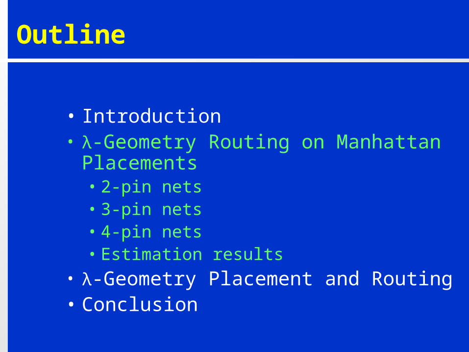
Outline

• Introduction• λ-Geometry Routing on Manhattan

Placements• λ-Geometry Placement and Routing

• Conclusion

Outline

• Introduction• Motivation• Previous estimation methods• Summary of previous results

• λ-Geometry Routing on Manhattan Placements

• λ-Geometry Placement and Routing

• Conclusion

Motivation

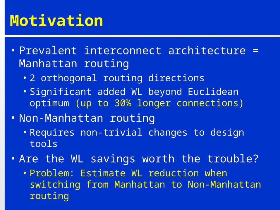
• Prevalent interconnect architecture = Manhattan routing• 2 orthogonal routing directions• Significant added WL beyond Euclidean optimum

(up to 30% longer connections)

• Non-Manhattan routing• Requires non-trivial changes to design tools

• Are the WL savings worth the trouble?• Problem: Estimate WL reduction when switching

from Manhattan to Non-Manhattan routing

λ-Geometry Routing

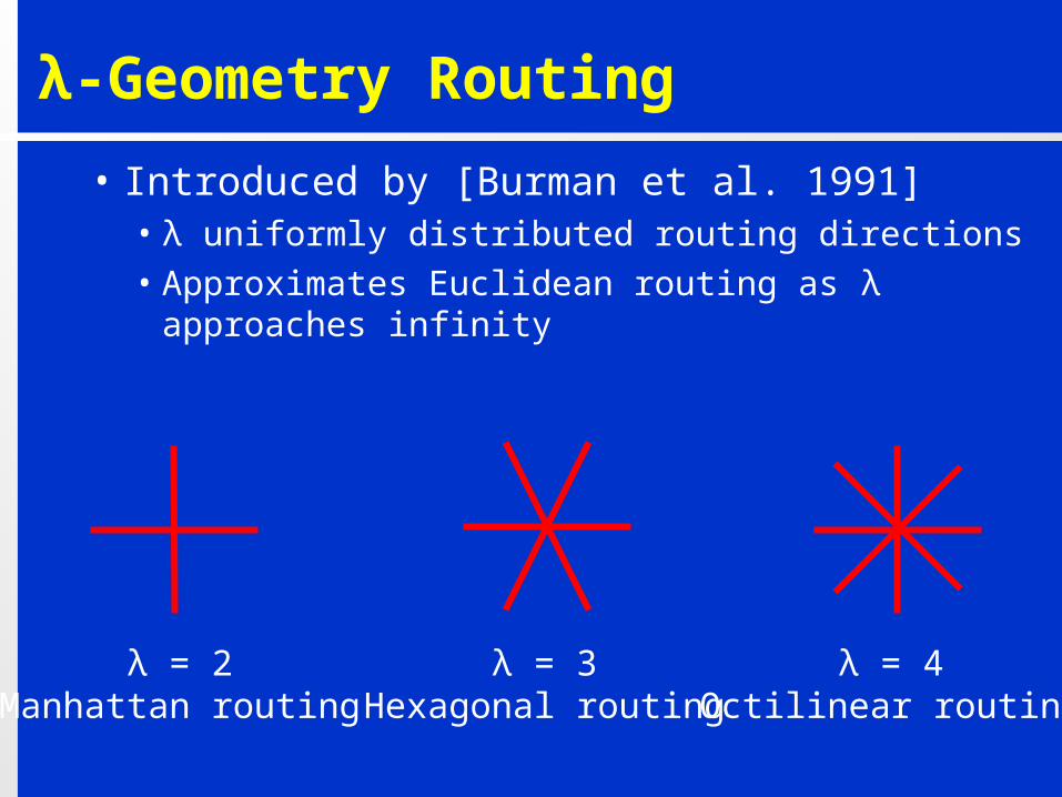
• Introduced by [Burman et al. 1991]• λ uniformly distributed routing directions• Approximates Euclidean routing as λ

approaches infinity

λ = 2Manhattan routing

λ = 4Octilinear routing

λ = 3Hexagonal routing

Previous Estimates (I)

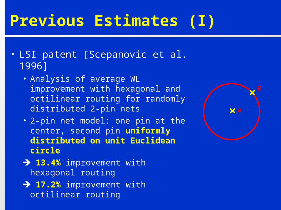
• LSI patent [Scepanovic et al. 1996]• Analysis of average WL improvement

with hexagonal and octilinear routing for randomly distributed 2-pin nets

• 2-pin net model: one pin at the center, second pin uniformly distributed on unit Euclidean circle

13.4% improvement with hexagonal routing

17.2% improvement with octilinear routing

A

B

Previous Estimates (II)

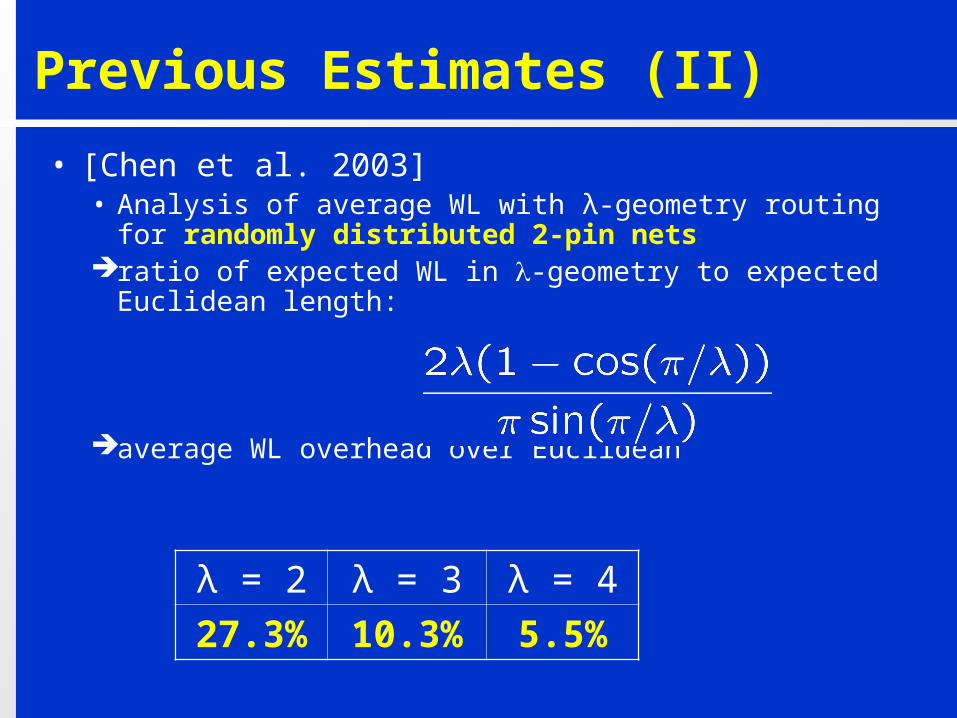
• [Chen et al. 2003]• Analysis of average WL with λ-geometry routing for randomly

distributed 2-pin netsratio of expected WL in -geometry to expected Euclidean

length:

average WL overhead over Euclidean

λ = 2 λ = 3 λ = 4

27.3% 10.3% 5.5%

Previous Estimates (III)

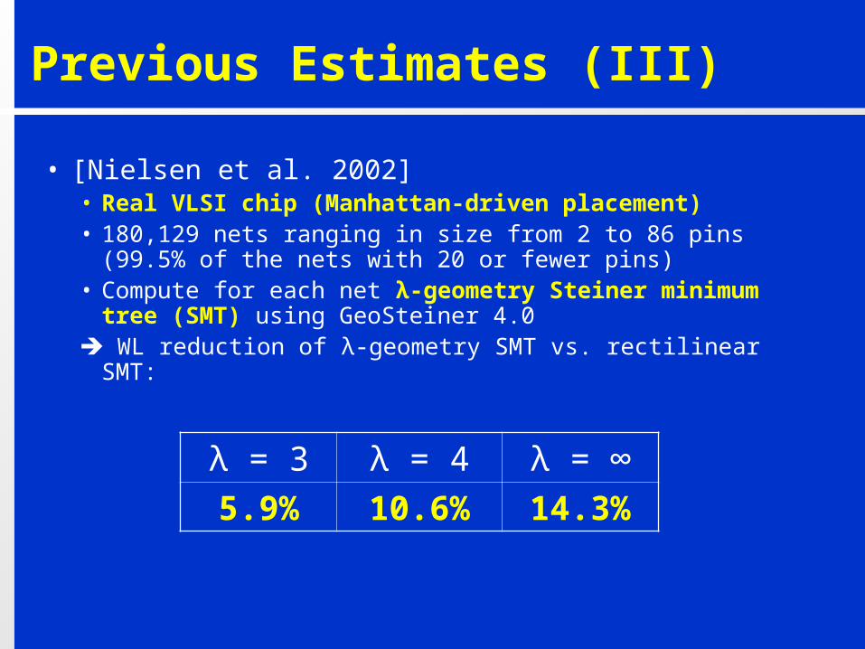
• [Nielsen et al. 2002]• Real VLSI chip (Manhattan-driven placement)• 180,129 nets ranging in size from 2 to 86 pins (99.5% of the

nets with 20 or fewer pins)• Compute for each net λ-geometry Steiner minimum tree

(SMT) using GeoSteiner 4.0 WL reduction of λ-geometry SMT vs. rectilinear SMT:

λ = 3 λ = 4 λ = ∞

5.9% 10.6% 14.3%

Previous Estimates (IV)

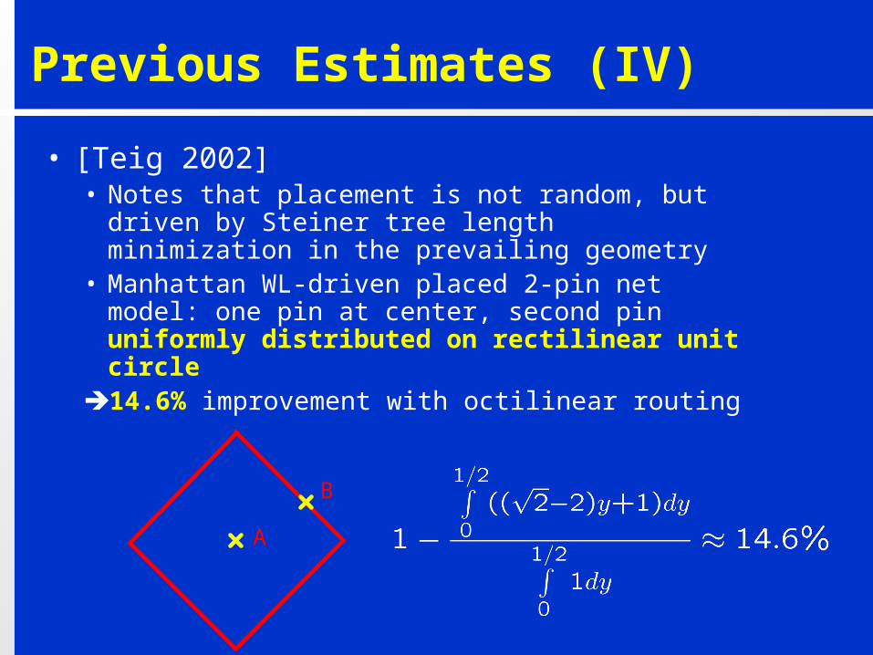
• [Teig 2002]• Notes that placement is not random, but driven by

Steiner tree length minimization in the prevailing geometry

• Manhattan WL-driven placed 2-pin net model: one pin at center, second pin uniformly distributed on rectilinear unit circle

14.6% improvement with octilinear routing

A

B

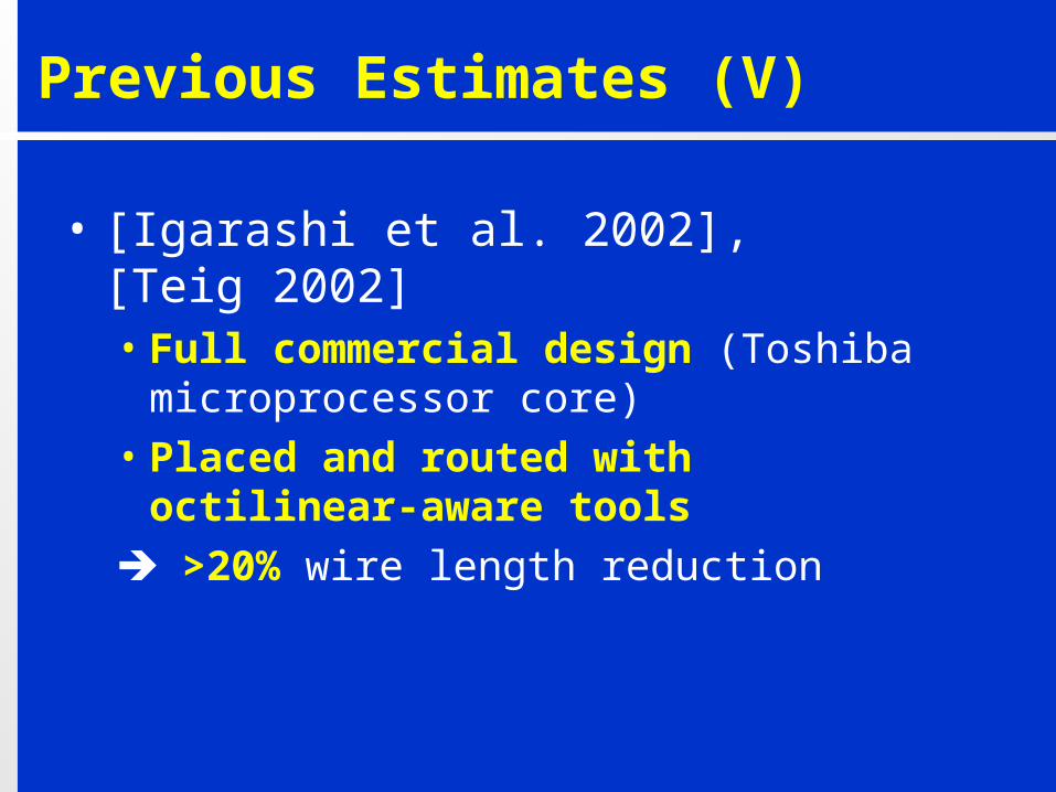
Previous Estimates (V)

• [Igarashi et al. 2002], [Teig 2002]• Full commercial design (Toshiba

microprocessor core)• Placed and routed with octilinear-

aware tools

>20% wire length reduction

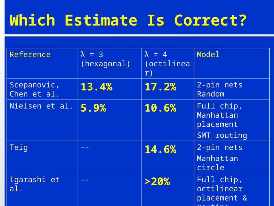
Which Estimate Is Correct?

Reference λ = 3 (hexagonal)

λ = 4 (octilinear)

Model

Scepanovic, Chen et al.

13.4% 17.2% 2-pin nets Random

Nielsen et al. 5.9% 10.6% Full chip, Manhattan placement

SMT routing

Teig -- 14.6% 2-pin nets

Manhattan circle

Igarashi et al. -- >20% Full chip, octilinear placement & routing

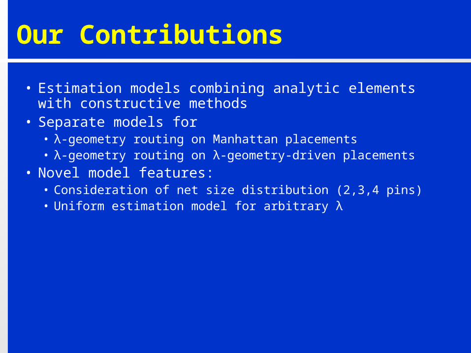
Our Contributions

• Estimation models combining analytic elements with constructive methods

• Separate models for• λ-geometry routing on Manhattan placements• λ-geometry routing on λ-geometry-driven placements

• Novel model features:• Consideration of net size distribution (2,3,4 pins)• Uniform estimation model for arbitrary λ

Outline

• Introduction• λ-Geometry Routing on Manhattan

Placements• 2-pin nets• 3-pin nets• 4-pin nets• Estimation results

• λ-Geometry Placement and Routing• Conclusion

λ-Geometry Routing on Manhattan Placements

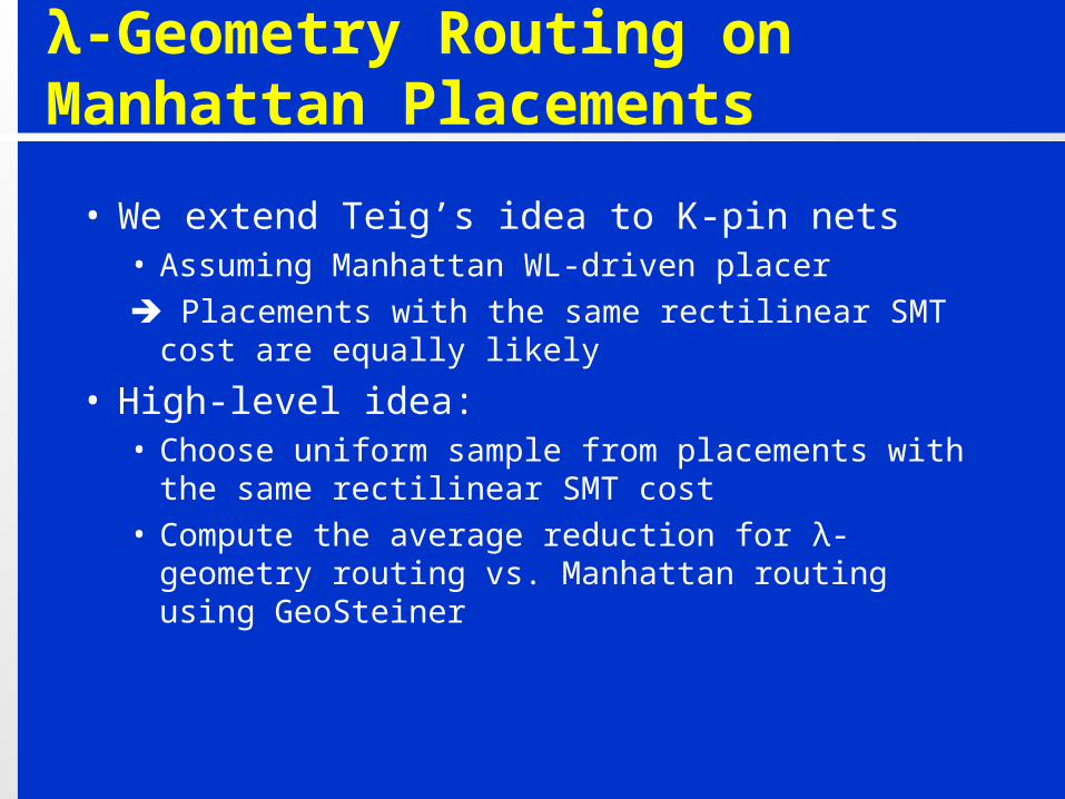
• We extend Teig’s idea to K-pin nets • Assuming Manhattan WL-driven placer

Placements with the same rectilinear SMT cost are equally likely

• High-level idea:• Choose uniform sample from placements with the

same rectilinear SMT cost• Compute the average reduction for λ-geometry

routing vs. Manhattan routing using GeoSteiner

2-Pin Nets

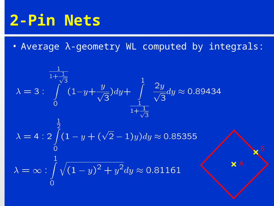
• Average λ-geometry WL computed by integrals:

A

B

v

u

3-Pin Nets (I)

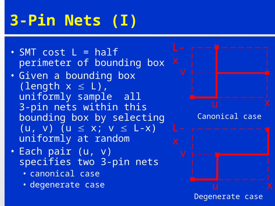
• SMT cost L = half perimeter of bounding box

• Given a bounding box (length x L), uniformly sample all 3-pin nets within this bounding box by selecting (u, v) (u x; v L-x) uniformly at random

• Each pair (u, v) specifies two 3-pin nets• canonical case• degenerate case

Degenerate case

Canonical case

v

u

x

L-x

x

L-x

3-Pin Nets (II)

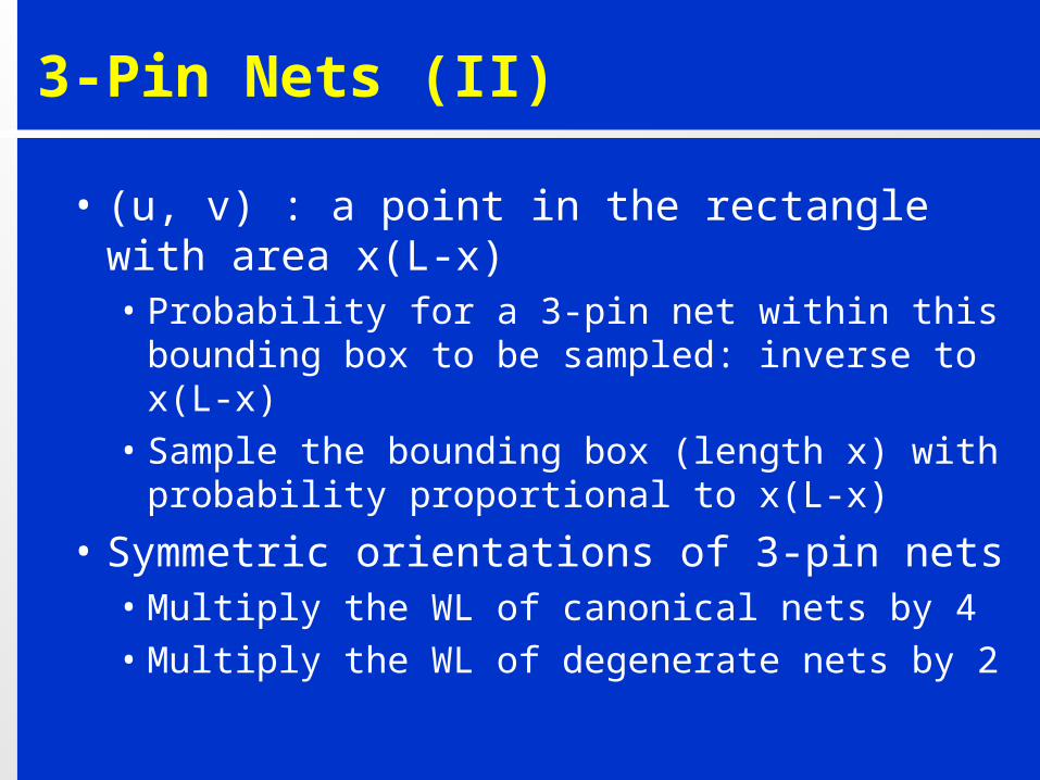
• (u, v) : a point in the rectangle with area x(L-x)• Probability for a 3-pin net within this bounding

box to be sampled: inverse to x(L-x)• Sample the bounding box (length x) with

probability proportional to x(L-x)

• Symmetric orientations of 3-pin nets• Multiply the WL of canonical nets by 4• Multiply the WL of degenerate nets by 2

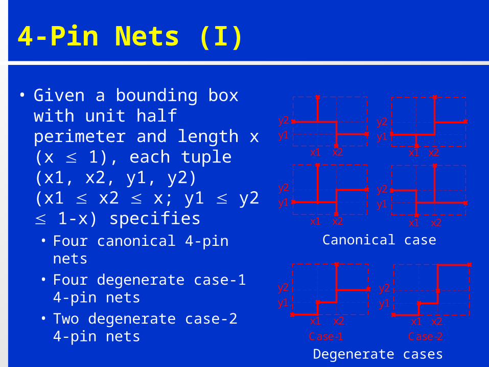
4-Pin Nets (I)

• Given a bounding box with unit half perimeter and length x (x 1), each tuple (x1, x2, y1, y2) (x1 x2 x; y1 y2 1-x) specifies• Four canonical 4-pin nets• Four degenerate case-1

4-pin nets• Two degenerate case-2

4-pin nets

Degenerate cases

Canonical case

x1 x2

y1

y2

y1

y2

y1

y2

y1

y2

x1 x2x1 x2

x1 x2

y1

x1 x2

y2

y1

x1 x2

y2

Case-1 Case-2

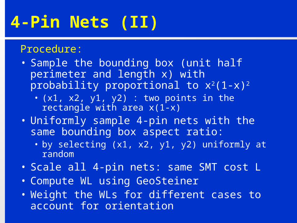
4-Pin Nets (II)

Procedure: • Sample the bounding box (unit half perimeter

and length x) with probability proportional to x2(1-x)2

• (x1, x2, y1, y2) : two points in the rectangle with area x(1-x)

• Uniformly sample 4-pin nets with the same bounding box aspect ratio: • by selecting (x1, x2, y1, y2) uniformly at random

• Scale all 4-pin nets: same SMT cost L• Compute WL using GeoSteiner• Weight the WLs for different cases to account

for orientation

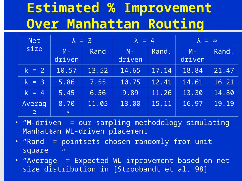
Estimated % Improvement Over Manhattan Routing

• “M-driven” = our sampling methodology simulating Manhattan WL-driven placement

• “Rand” = pointsets chosen randomly from unit square• “Average” = Expected WL improvement based on net size

distribution in [Stroobandt et al. 98]

Net size λ = 3 λ = 4 λ = ∞

M-driven Rand M-driven Rand. M-driven Rand.

k = 2 10.57 13.52 14.65 17.14 18.84 21.47

k = 3 5.86 7.55 10.75 12.41 14.61 16.21

k = 4 5.45 6.56 9.89 11.26 13.30 14.80

Average 8.70 11.05 13.00 15.11 16.97 19.19

Outline

• Introduction• λ-Geometry Routing on Manhattan

Placements• λ-Geometry Placement and Routing

• Simulated annealing placer• Estimation results

• Conclusion

λ-Geometry Placement and Routing

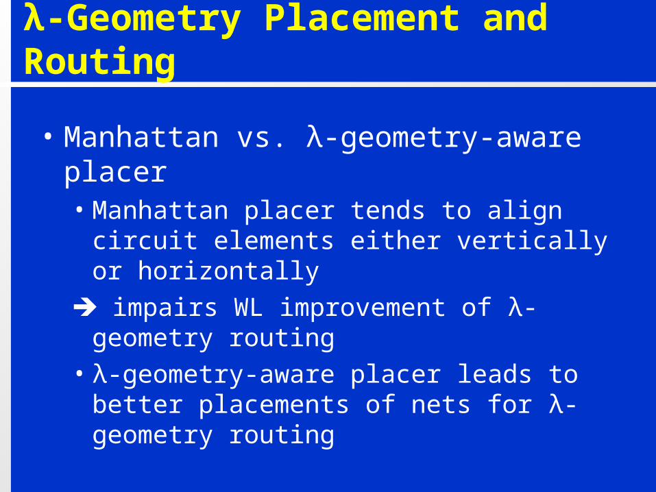
• Manhattan vs. λ-geometry-aware placer• Manhattan placer tends to align circuit

elements either vertically or horizontally

impairs WL improvement of λ-geometry routing

• λ-geometry-aware placer leads to better placements of nets for λ-geometry routing

Simulated Annealing Placer

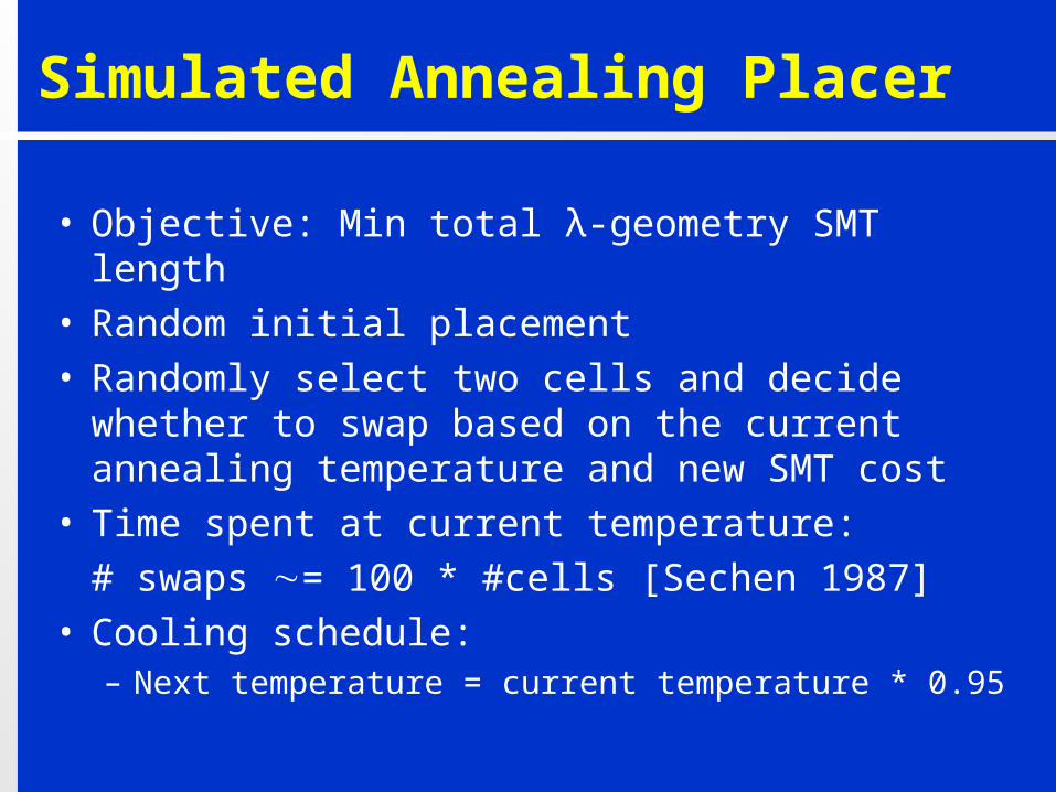
• Objective: Min total λ-geometry SMT length• Random initial placement• Randomly select two cells and decide whether to

swap based on the current annealing temperature and new SMT cost

• Time spent at current temperature:

# swaps = 100 * #cells [Sechen 1987] • Cooling schedule:

– Next temperature = current temperature * 0.95

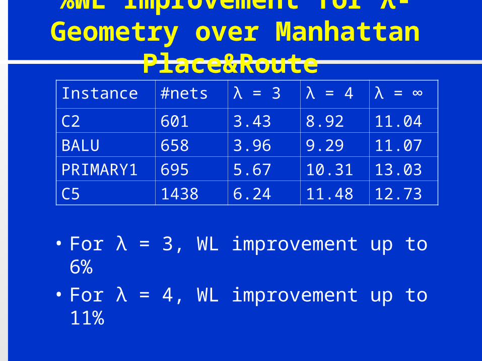
%WL Improvement for λ-Geometry over Manhattan Place&Route

• For λ = 3, WL improvement up to 6%

• For λ = 4, WL improvement up to 11%

Instance #nets λ = 3 λ = 4 λ = ∞

C2 601 3.43 8.92 11.04

BALU 658 3.96 9.29 11.07

PRIMARY1 695 5.67 10.31 13.03

C5 1438 6.24 11.48 12.73

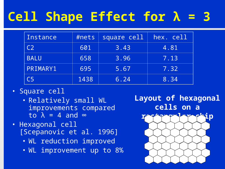
Cell Shape Effect for λ = 3

• Square cell• Relatively small WL

improvements compared to λ = 4 and ∞

• Hexagonal cell [Scepanovic et al. 1996]• WL reduction improved• WL improvement up to 8%

Layout of hexagonal cells on a

rectangular chip

Instance #nets square cell hex. cell

C2 601 3.43 4.81

BALU 658 3.96 7.13

PRIMARY1 695 5.67 7.32

C5 1438 6.24 8.34

“Virtuous Cycle” Effect (I)

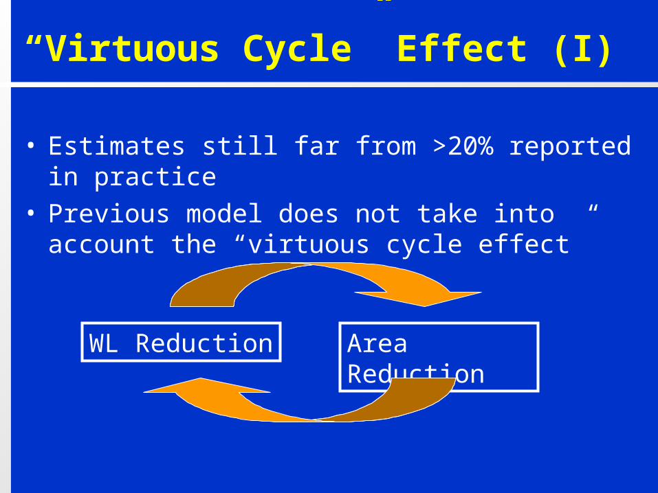
• Estimates still far from >20% reported in practice• Previous model does not take into account the

“virtuous cycle effect”

WL Reduction Area Reduction

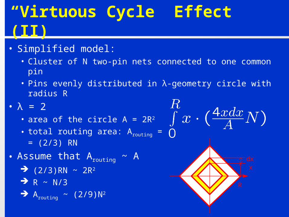
“Virtuous Cycle” Effect (II)

• Simplified model: • Cluster of N two-pin nets connected to one common pin • Pins evenly distributed in λ-geometry circle with radius R

• λ = 2 • area of the circle A = 2R2

• total routing area: Arouting = = (2/3) RN

• Assume that Arouting ~ A (2/3)RN ~ 2R2

R ~ N/3 Arouting ~ (2/9)N2

xdx

R

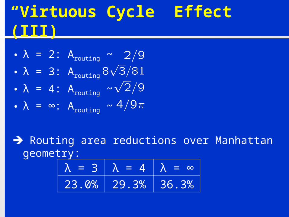
“Virtuous Cycle” Effect (III)

• λ = 2: Arouting ~ N2

• λ = 3: Arouting ~ N2

• λ = 4: Arouting ~ N2

• λ = ∞: Arouting ~ N2

Routing area reductions over Manhattan geometry:

λ = 3 λ = 4 λ = ∞

23.0% 29.3% 36.3%

Conclusions

• Proposed more accurate estimation models for WL reduction of λ-geometry routing vs. Manhattan routing• Effect of placement (Manhattan vs. λ-geometry-

driven placement)• Net size distribution• Virtuous cycle effect

• Ongoing work:• More accurate model for λ-geometry-driven

placement

Thank You !