Doktorandenseminar 2003: QED 2 - INFNsmueller/talks/QED_seminar.pdf · Doktorandenseminar 2003: QED...
74
Doktorandenseminar 2003: QED 2 Calculating the e + e - → μ + μ - cross section γ e - e + μ + μ - Stefan E. M ¨ uller November 24, 2003 . – p.1
-
Upload
trinhnguyet -
Category
Documents
-
view
227 -
download
1
Transcript of Doktorandenseminar 2003: QED 2 - INFNsmueller/talks/QED_seminar.pdf · Doktorandenseminar 2003: QED...
Doktorandenseminar2003: QED 2
Calculating the e+e− → µ+µ− cross
section
γ
e−
e+ µ+
µ−
Stefan E. Muller
November 24, 2003
. – p.1
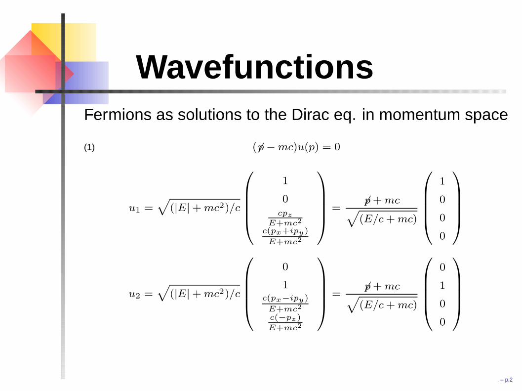
WavefunctionsFermions as solutions to the Dirac eq. in momentum space
(6p−mc)u(p) = 0(1)
u1 =√
(|E|+ mc2)/c
1
0cpz
E+mc2
c(px+ipy)
E+mc2
=6p + mc√
(E/c + mc)
1
0
0
0
u2 =√
(|E|+ mc2)/c
0
1c(px−ipy)
E+mc2
c(−pz)
E+mc2
=6p + mc√
(E/c + mc)
0
1
0
0
. – p.2
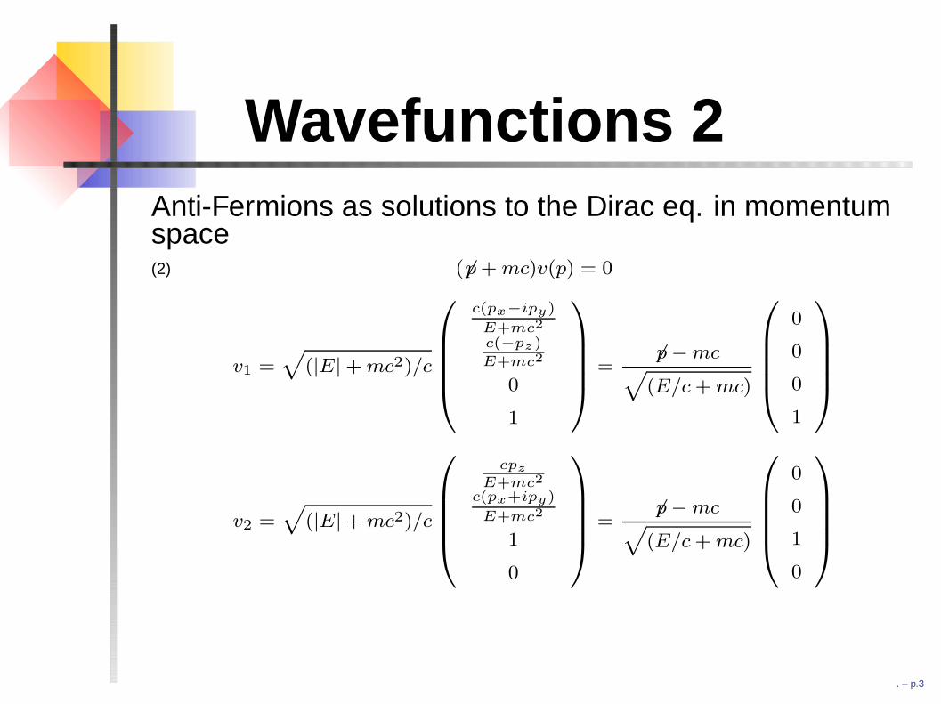
Wavefunctions 2Anti-Fermions as solutions to the Dirac eq. in momentumspace
(6p + mc)v(p) = 0(2)
v1 =√
(|E|+ mc2)/c
c(px−ipy)
E+mc2
c(−pz)
E+mc2
0
1
=6p−mc√
(E/c + mc)
0
0
0
1
v2 =√
(|E|+ mc2)/c
cpz
E+mc2
c(px+ipy)
E+mc2
1
0
=6p−mc√
(E/c + mc)
0
0
1
0
. – p.3
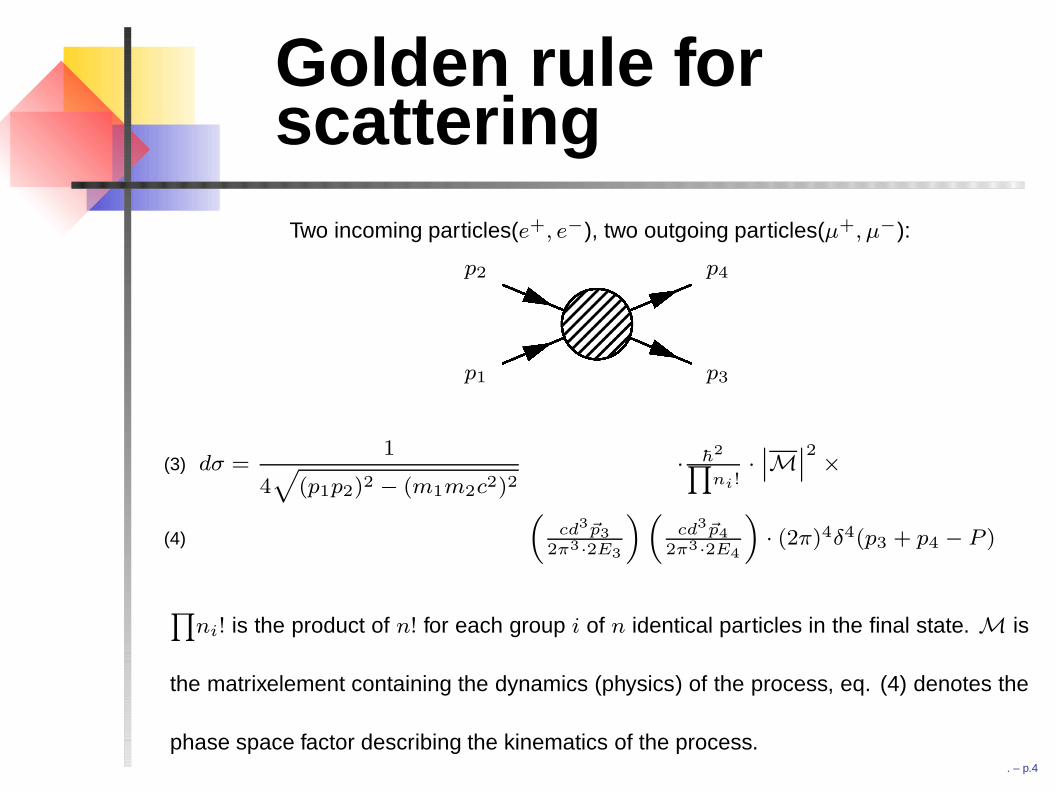
Golden rule forscattering
Two incoming particles(e+, e−), two outgoing particles(µ+, µ−):
p1
p2
p3
p4
dσ =1
4√
(p1p2)2 − (m1m2c2)2· h2∏
ni!·∣∣M
∣∣2 ×(3)
(cd3~p3
2π3·2E3
)(cd3~p4
2π3·2E4
)· (2π)4δ4(p3 + p4 − P )(4)
∏ni! is the product of n! for each group i of n identical particles in the final state. M is
the matrixelement containing the dynamics (physics) of the process, eq. (4) denotes the
phase space factor describing the kinematics of the process.. – p.4
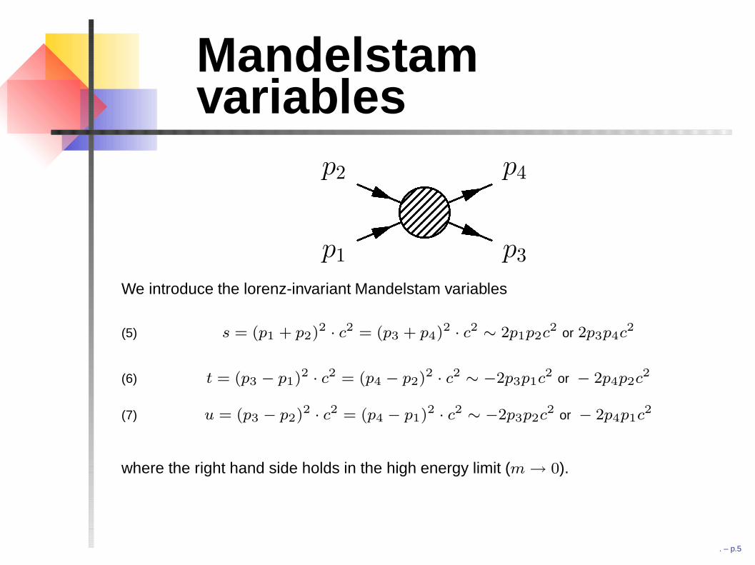
Mandelstamvariables
p1
p2
p3
p4
We introduce the lorenz-invariant Mandelstam variables
s = (p1 + p2)2 · c2 = (p3 + p4)2 · c2 ∼ 2p1p2c2 or 2p3p4c2(5)
t = (p3 − p1)2 · c2 = (p4 − p2)
2 · c2 ∼ −2p3p1c2 or − 2p4p2c2(6)
u = (p3 − p2)2 · c2 = (p4 − p1)2 · c2 ∼ −2p3p2c2 or − 2p4p1c2(7)
where the right hand side holds in the high energy limit (m→ 0).
. – p.5
Mandelstamvariables 2
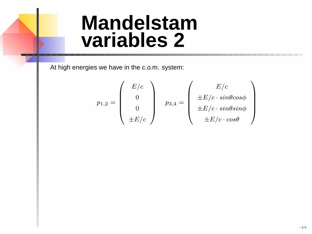
At high energies we have in the c.o.m. system:
p1,2 =
E/c
0
0
±E/c
p3,4 =
E/c
±E/c · sinθcosφ
±E/c · sinθsinφ
±E/c · cosθ
The Mandelstam variables then become
s = 4E2(8)
t = −s
2(1− cosθ)(9)
u = −s
2(1 + cosθ)(10)
. – p.6
Mandelstamvariables 2
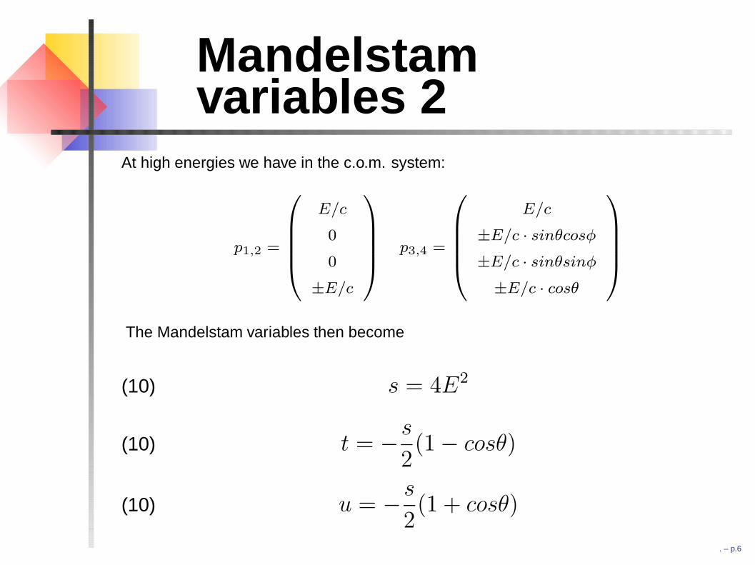
At high energies we have in the c.o.m. system:
p1,2 =
E/c
0
0
±E/c
p3,4 =
E/c
±E/c · sinθcosφ
±E/c · sinθsinφ
±E/c · cosθ
The Mandelstam variables then become
s = 4E2(10)
t = −s
2(1− cosθ)(10)
u = −s
2(1 + cosθ)(10)
. – p.6
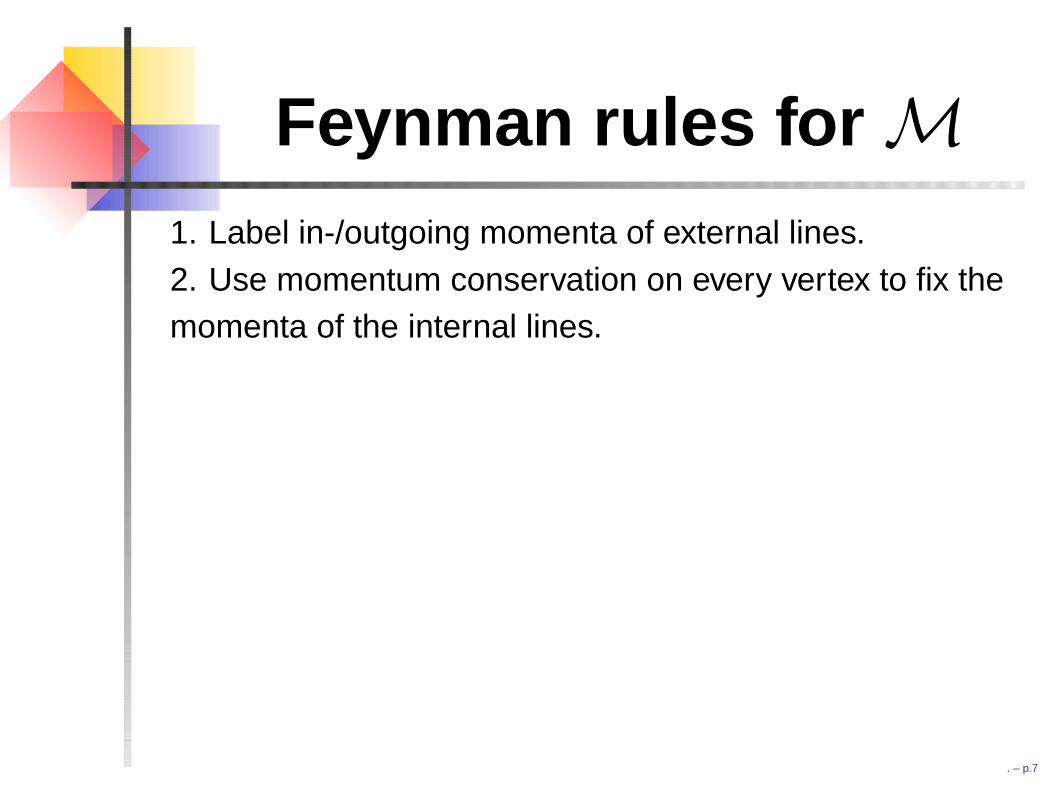
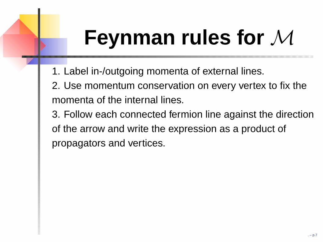
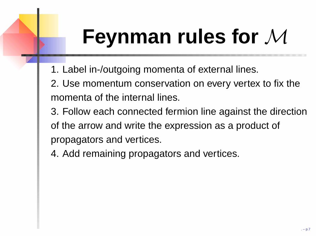
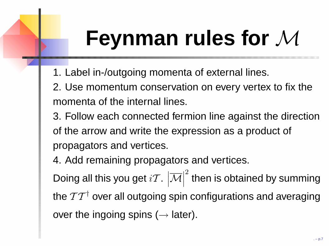
Feynman rules for M
1. Label in-/outgoing momenta of external lines.2. Use momentum conservation on every vertex to fix themomenta of the internal lines.3. Follow each connected fermion line against the directionof the arrow and write the expression as a product ofpropagators and vertices.4. Add remaining propagators and vertices.
Doing all this you get iT .∣∣∣M
∣∣∣2
then is obtained by summing
the T T † over all outgoing spin configurations and averaging
over the ingoing spins (→ later).
. – p.7
Feynman rules for M1. Label in-/outgoing momenta of external lines.
2. Use momentum conservation on every vertex to fix themomenta of the internal lines.3. Follow each connected fermion line against the directionof the arrow and write the expression as a product ofpropagators and vertices.4. Add remaining propagators and vertices.
Doing all this you get iT .∣∣∣M
∣∣∣2
then is obtained by summing
the T T † over all outgoing spin configurations and averaging
over the ingoing spins (→ later).
. – p.7
Feynman rules for M1. Label in-/outgoing momenta of external lines.2. Use momentum conservation on every vertex to fix themomenta of the internal lines.
3. Follow each connected fermion line against the directionof the arrow and write the expression as a product ofpropagators and vertices.4. Add remaining propagators and vertices.
Doing all this you get iT .∣∣∣M
∣∣∣2
then is obtained by summing
the T T † over all outgoing spin configurations and averaging
over the ingoing spins (→ later).
. – p.7
Feynman rules for M1. Label in-/outgoing momenta of external lines.2. Use momentum conservation on every vertex to fix themomenta of the internal lines.3. Follow each connected fermion line against the directionof the arrow and write the expression as a product ofpropagators and vertices.
4. Add remaining propagators and vertices.
Doing all this you get iT .∣∣∣M
∣∣∣2
then is obtained by summing
the T T † over all outgoing spin configurations and averaging
over the ingoing spins (→ later).
. – p.7
Feynman rules for M1. Label in-/outgoing momenta of external lines.2. Use momentum conservation on every vertex to fix themomenta of the internal lines.3. Follow each connected fermion line against the directionof the arrow and write the expression as a product ofpropagators and vertices.4. Add remaining propagators and vertices.
Doing all this you get iT .∣∣∣M
∣∣∣2
then is obtained by summing
the T T † over all outgoing spin configurations and averaging
over the ingoing spins (→ later).
. – p.7
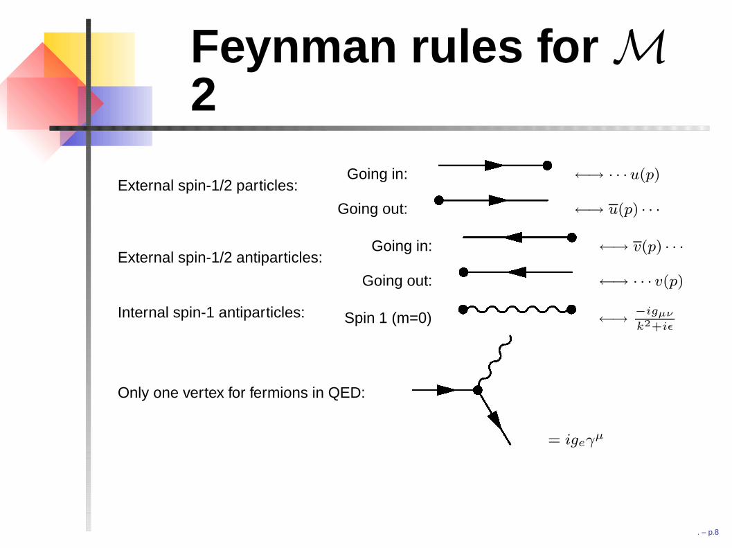
Feynman rules for M2
External spin-1/2 particles:Going in: ←→ · · ·u(p)
Going out: ←→ u(p) · · ·
External spin-1/2 antiparticles:Going in: ←→ v(p) · · ·
Going out: ←→ · · · v(p)
Internal spin-1 antiparticles: Spin 1 (m=0) ←→ −igµν
k2+iε
Only one vertex for fermions in QED:
= igeγµ
. – p.8

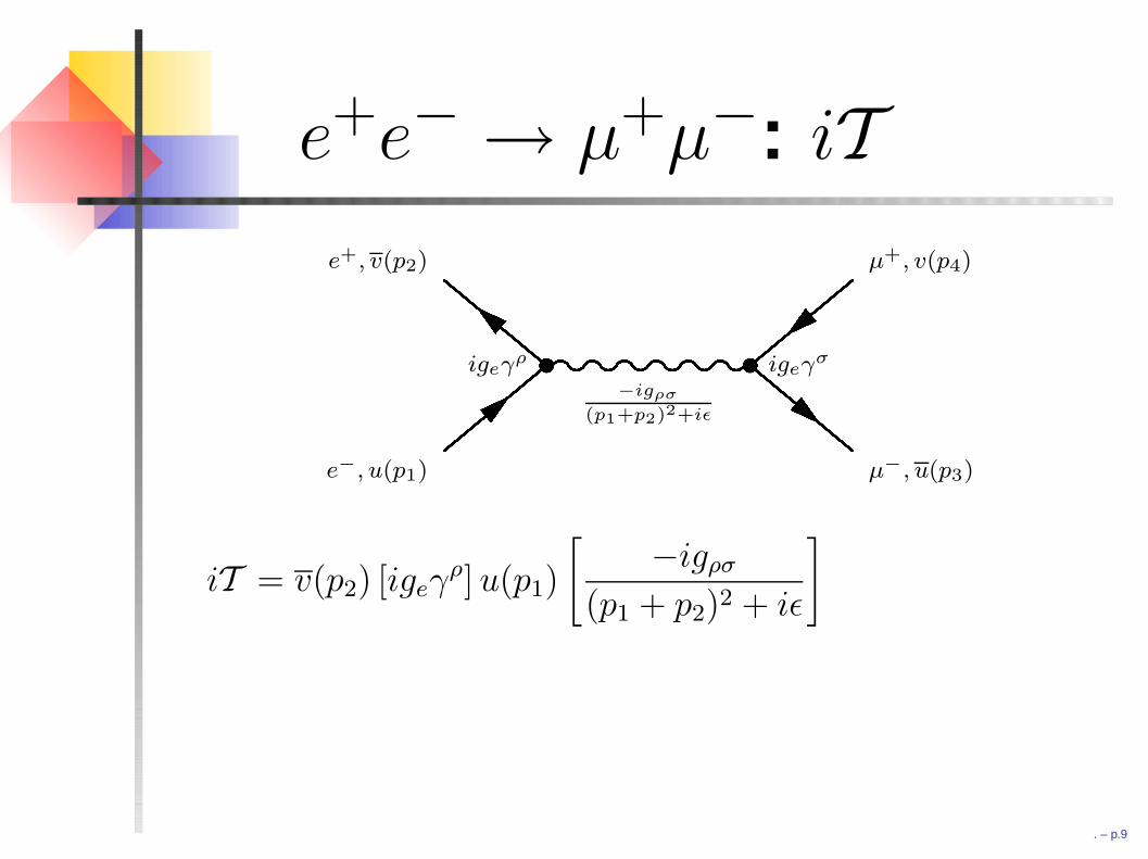
e+e− → µ+µ−: iT
−igρσ
(p1+p2)2+iε
e−, u(p1)
e+, v(p2)
igeγρ igeγσ
µ+, v(p4)
µ−, u(p3)
iT =
v(p2) [igeγρ]u(p1)
[−igρσ
(p1 + p2)2 + iε
]u(p3) [igeγ
σ] v(p4)
iε→0= ig2
e ·c2
s[v(p2)γσu(p1)] · [u(p3)γ
σv(p4)]
. – p.9

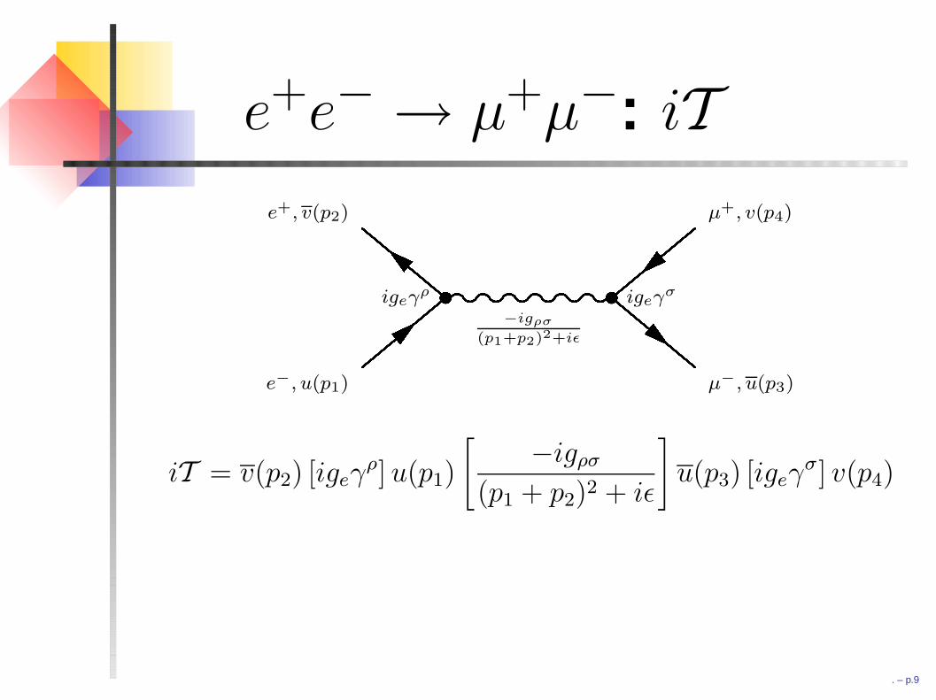
e+e− → µ+µ−: iT
−igρσ
(p1+p2)2+iε
e−, u(p1)
e+, v(p2)
igeγρ igeγσ
µ+, v(p4)
µ−, u(p3)
iT = v(p2) [igeγρ]u(p1)
[−igρσ
(p1 + p2)2 + iε
]u(p3) [igeγ
σ] v(p4)
iε→0= ig2
e ·c2
s[v(p2)γσu(p1)] · [u(p3)γ
σv(p4)]
. – p.9
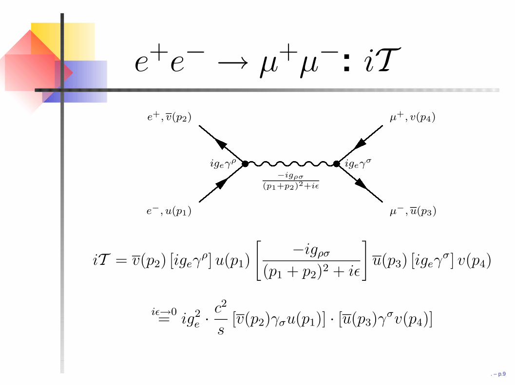
e+e− → µ+µ−: iT
−igρσ
(p1+p2)2+iε
e−, u(p1)
e+, v(p2)
igeγρ igeγσ
µ+, v(p4)
µ−, u(p3)
iT = v(p2) [igeγρ] u(p1)
[−igρσ
(p1 + p2)2 + iε
]
u(p3) [igeγσ] v(p4)
iε→0= ig2
e ·c2
s[v(p2)γσu(p1)] · [u(p3)γ
σv(p4)]
. – p.9
e+e− → µ+µ−: iT
−igρσ
(p1+p2)2+iε
e−, u(p1)
e+, v(p2)
igeγρ igeγσ
µ+, v(p4)
µ−, u(p3)
iT = v(p2) [igeγρ] u(p1)
[−igρσ
(p1 + p2)2 + iε
]u(p3) [igeγ
σ] v(p4)
iε→0= ig2
e ·c2
s[v(p2)γσu(p1)] · [u(p3)γ
σv(p4)]
. – p.9
e+e− → µ+µ−: iT
−igρσ
(p1+p2)2+iε
e−, u(p1)
e+, v(p2)
igeγρ igeγσ
µ+, v(p4)
µ−, u(p3)
iT = v(p2) [igeγρ] u(p1)
[−igρσ
(p1 + p2)2 + iε
]u(p3) [igeγ
σ] v(p4)
iε→0= ig2
e ·c2
s[v(p2)γσu(p1)] · [u(p3)γ
σv(p4)]
. – p.9
Calculating |T |2
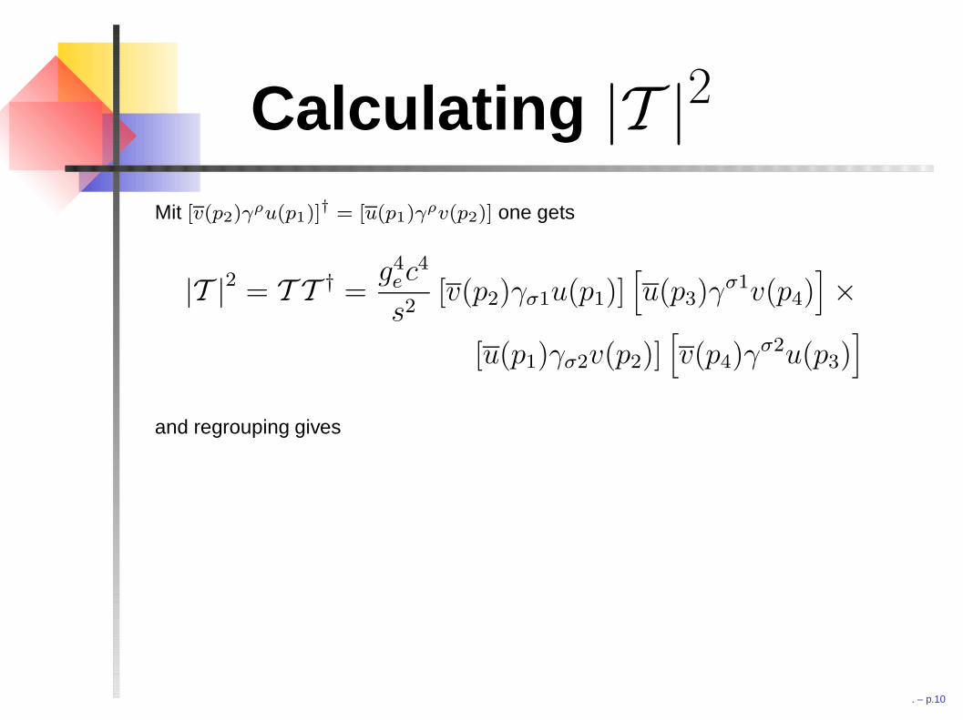
Mit [v(p2)γρu(p1)]† = [u(p1)γρv(p2)] one gets
|T |2 = T T † =g4
ec4
s2[v(p2)γσ1u(p1)]
[u(p3)γ
σ1v(p4)]×
[u(p1)γσ2v(p2)][v(p4)γ
σ2u(p3)]
and regrouping gives
=g4
ec4
s2[v(p2)γσ1u(p1)u(p1)γσ2v(p2)]×
[u(p3)γ
σ1v(p4)v(p4)γσ2u(p3)
]
Note that expressions of the form uγσv are just numbers.
. – p.10
Calculating |T |2
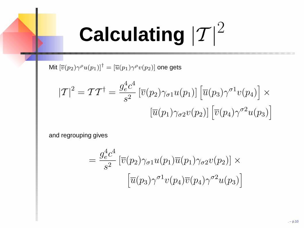
Mit [v(p2)γρu(p1)]† = [u(p1)γρv(p2)] one gets
|T |2 = T T † =g4
ec4
s2[v(p2)γσ1u(p1)]
[u(p3)γ
σ1v(p4)]×
[u(p1)γσ2v(p2)][v(p4)γ
σ2u(p3)]
and regrouping gives
=g4
ec4
s2[v(p2)γσ1u(p1)u(p1)γσ2v(p2)]×
[u(p3)γ
σ1v(p4)v(p4)γσ2u(p3)
]
Note that expressions of the form uγσv are just numbers.
. – p.10
Calculating |T |2
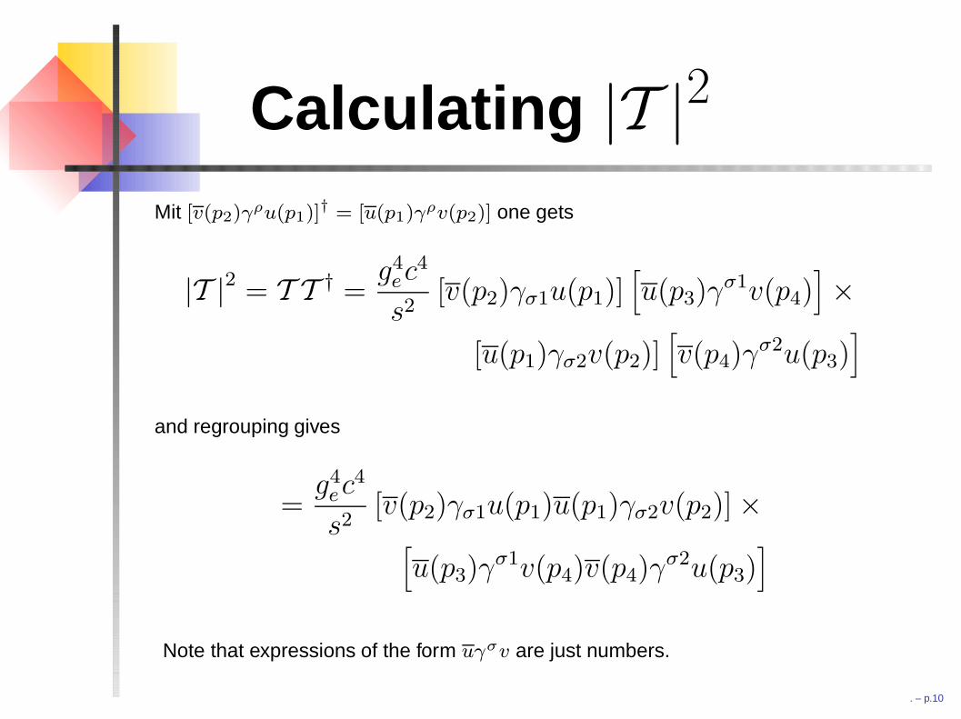
Mit [v(p2)γρu(p1)]† = [u(p1)γρv(p2)] one gets
|T |2 = T T † =g4
ec4
s2[v(p2)γσ1u(p1)]
[u(p3)γ
σ1v(p4)]×
[u(p1)γσ2v(p2)][v(p4)γ
σ2u(p3)]
and regrouping gives
=g4
ec4
s2[v(p2)γσ1u(p1)u(p1)γσ2v(p2)]×
[u(p3)γ
σ1v(p4)v(p4)γσ2u(p3)
]
Note that expressions of the form uγσv are just numbers.
. – p.10

Summing over spins(Casimir’s trick)
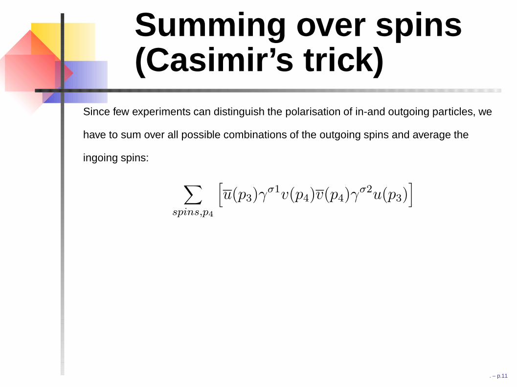
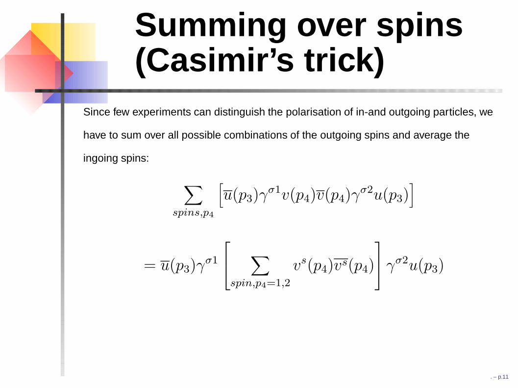
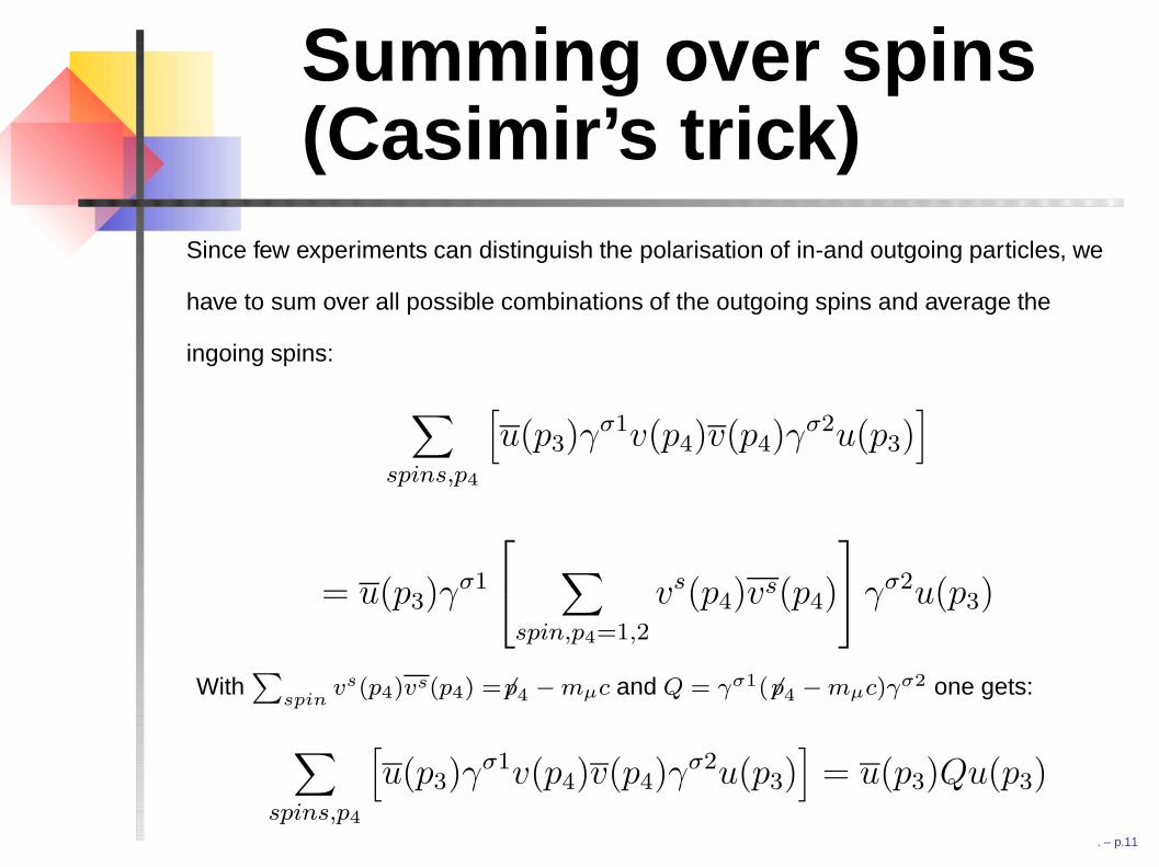
Since few experiments can distinguish the polarisation of in-and outgoing particles, we
have to sum over all possible combinations of the outgoing spins and average the
ingoing spins:
∑
spins,p4
[u(p3)γ
σ1v(p4)v(p4)γσ2u(p3)
]
= u(p3)γσ1
∑
spin,p4=1,2
vs(p4)vs(p4)
γσ2u(p3)
With∑
spinvs(p4)vs(p4) =6p4 −mµc and Q = γσ1(6p4 −mµc)γσ2 one gets:
∑
spins,p4
[u(p3)γ
σ1v(p4)v(p4)γσ2u(p3)
]= u(p3)Qu(p3)
. – p.11
Summing over spins(Casimir’s trick)
Since few experiments can distinguish the polarisation of in-and outgoing particles, we
have to sum over all possible combinations of the outgoing spins and average the
ingoing spins:
∑
spins,p4
[u(p3)γ
σ1v(p4)v(p4)γσ2u(p3)
]
= u(p3)γσ1
∑
spin,p4=1,2
vs(p4)vs(p4)
γσ2u(p3)
With∑
spinvs(p4)vs(p4) =6p4 −mµc and Q = γσ1(6p4 −mµc)γσ2 one gets:
∑
spins,p4
[u(p3)γ
σ1v(p4)v(p4)γσ2u(p3)
]= u(p3)Qu(p3)
. – p.11
Summing over spins(Casimir’s trick) 2
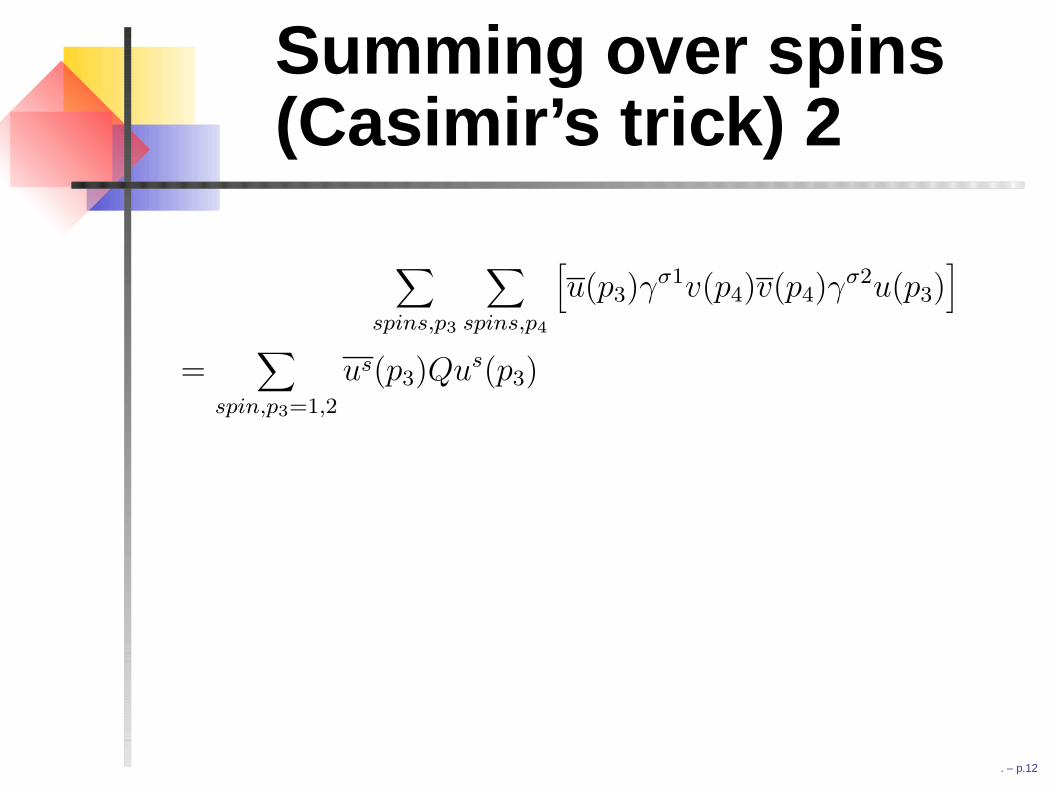
∑
spins,p3
∑
spins,p4
[u(p3)γ
σ1v(p4)v(p4)γσ2u(p3)
]
=∑
spin,p3=1,2
us(p3)Qus(p3)
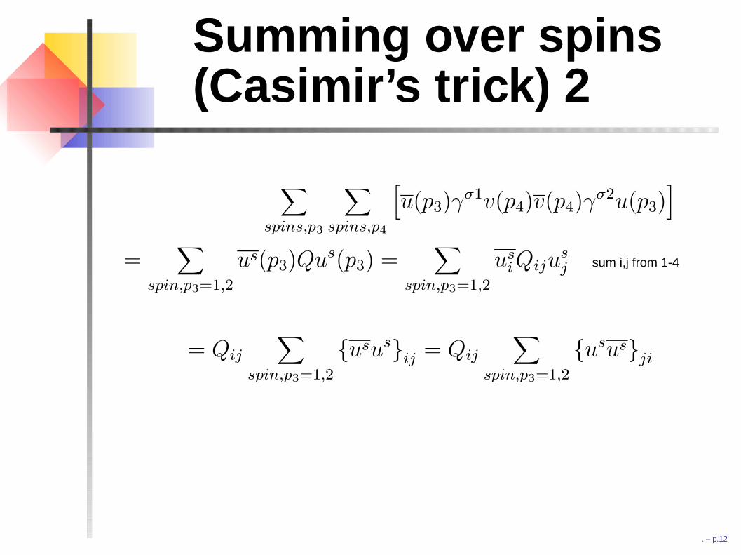
=∑
spin,p3=1,2
usiQiju
sj sum i,j from 1-4
= Qij
∑
spin,p3=1,2
ususij = Qij
∑
spin,p3=1,2
ususji
and with∑
spinus(p3)us(p3) =6p3 + mµc
= Qij6p3 + mµcji = Tr (Q(6p3 + mµc))
. – p.12

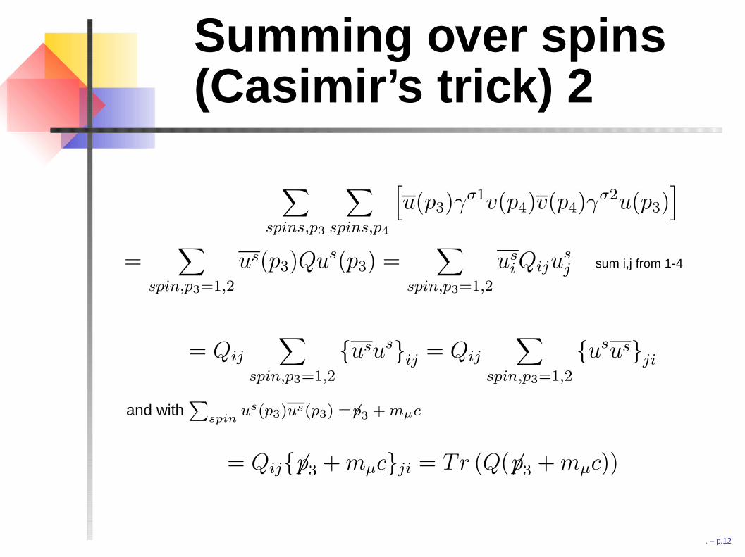
Summing over spins(Casimir’s trick) 2
∑
spins,p3
∑
spins,p4
[u(p3)γ
σ1v(p4)v(p4)γσ2u(p3)
]
=∑
spin,p3=1,2
us(p3)Qus(p3) =∑
spin,p3=1,2
usiQiju
sj sum i,j from 1-4
= Qij
∑
spin,p3=1,2
ususij = Qij
∑
spin,p3=1,2
ususji
and with∑
spinus(p3)us(p3) =6p3 + mµc
= Qij6p3 + mµcji = Tr (Q(6p3 + mµc))
. – p.12
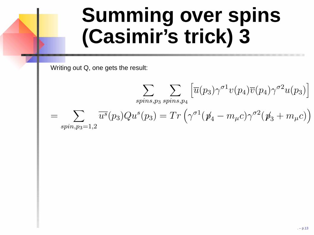
Summing over spins(Casimir’s trick) 3
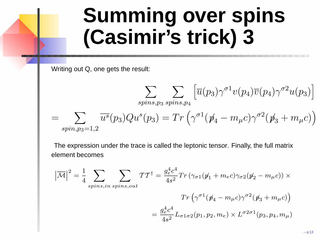
Writing out Q, one gets the result:
∑
spins,p3
∑
spins,p4
[u(p3)γ
σ1v(p4)v(p4)γσ2u(p3)
]
=∑
spin,p3=1,2
us(p3)Qus(p3) = Tr(γσ1(6p4 −mµc)γ
σ2(6p3 + mµc))
The expression under the trace is called the leptonic tensor. Finally, the full matrixelement becomes
∣∣M∣∣2 =
1
4
∑
spins,in
∑
spins,out
T T † =g4
ec4
4s2Tr (γσ1(6p1 + mec)γσ2(6p2 −mµc))×
Tr(γσ1(6p4 −mµc)γσ2(6p3 + mµc)
)
=g4
ec4
4s2Lσ1σ2(p1, p2, me)× Lσ2σ1(p3, p4, mµ)
. – p.13
Summing over spins(Casimir’s trick) 3
Writing out Q, one gets the result:
∑
spins,p3
∑
spins,p4
[u(p3)γ
σ1v(p4)v(p4)γσ2u(p3)
]
=∑
spin,p3=1,2
us(p3)Qus(p3) = Tr(γσ1(6p4 −mµc)γ
σ2(6p3 + mµc))
The expression under the trace is called the leptonic tensor. Finally, the full matrixelement becomes
∣∣M∣∣2 =
1
4
∑
spins,in
∑
spins,out
T T † =g4
ec4
4s2Tr (γσ1(6p1 + mec)γσ2(6p2 −mµc))×
Tr(γσ1(6p4 −mµc)γσ2(6p3 + mµc)
)
=g4
ec4
4s2Lσ1σ2(p1, p2, me)× Lσ2σ1(p3, p4, mµ)
. – p.13
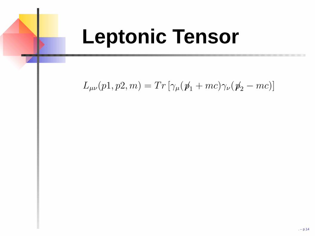
Leptonic Tensor
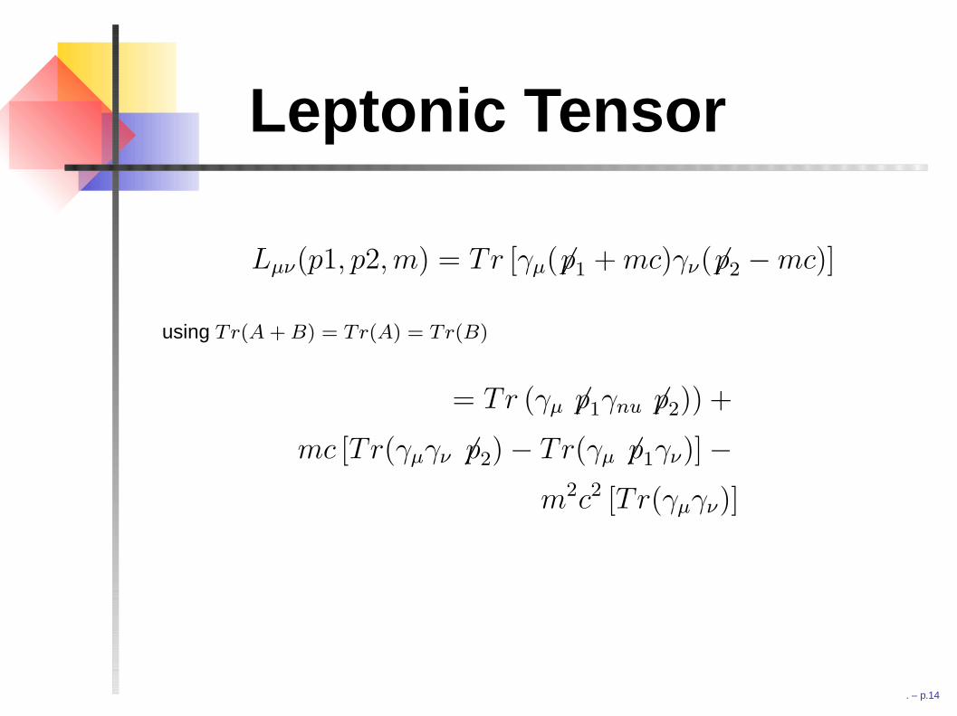
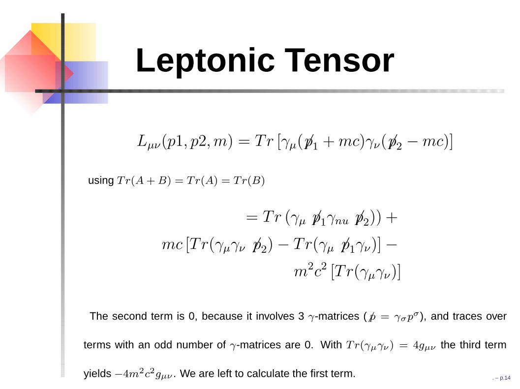
Lµν(p1, p2,m) = Tr [γµ(6p1 + mc)γν(6p2 −mc)]
using Tr(A + B) = Tr(A) = Tr(B)
= Tr (γµ 6p1γnu 6p2)) +
mc [Tr(γµγν 6 p2)− Tr(γµ 6 p1γν)]−
m2c2 [Tr(γµγν)]
The second term is 0, because it involves 3 γ-matrices (6 p = γσpσ), and traces over
terms with an odd number of γ-matrices are 0. With Tr(γµγν) = 4gµν the third term
yields −4m2c2gµν . We are left to calculate the first term.
. – p.14
Leptonic Tensor
Lµν(p1, p2,m) = Tr [γµ(6p1 + mc)γν(6p2 −mc)]
using Tr(A + B) = Tr(A) = Tr(B)
= Tr (γµ 6p1γnu 6p2)) +
mc [Tr(γµγν 6 p2)− Tr(γµ 6 p1γν)]−
m2c2 [Tr(γµγν)]
The second term is 0, because it involves 3 γ-matrices (6 p = γσpσ), and traces over
terms with an odd number of γ-matrices are 0. With Tr(γµγν) = 4gµν the third term
yields −4m2c2gµν . We are left to calculate the first term. . – p.14
Leptonic Tensor 2
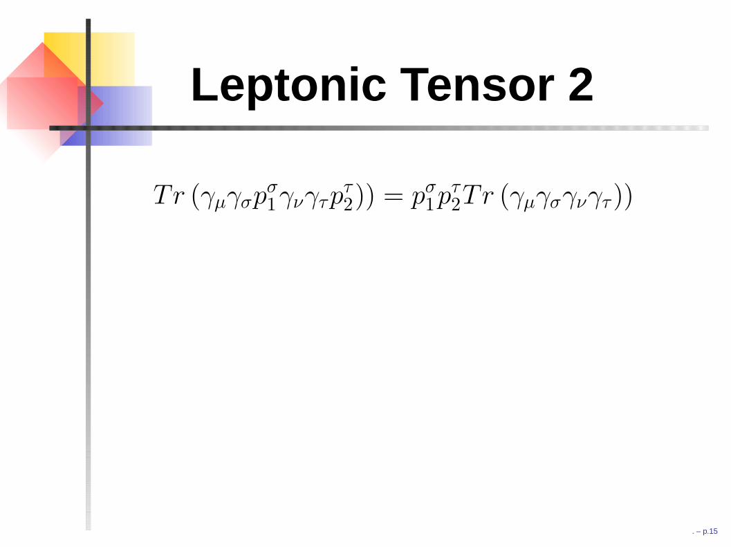
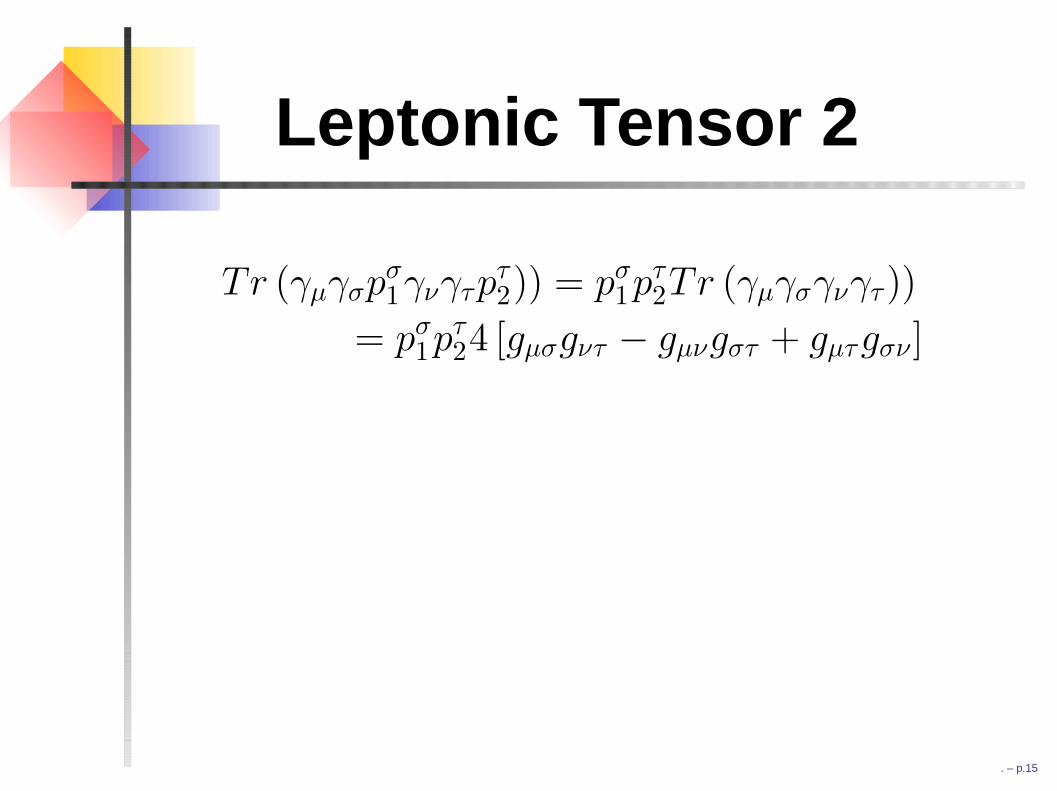
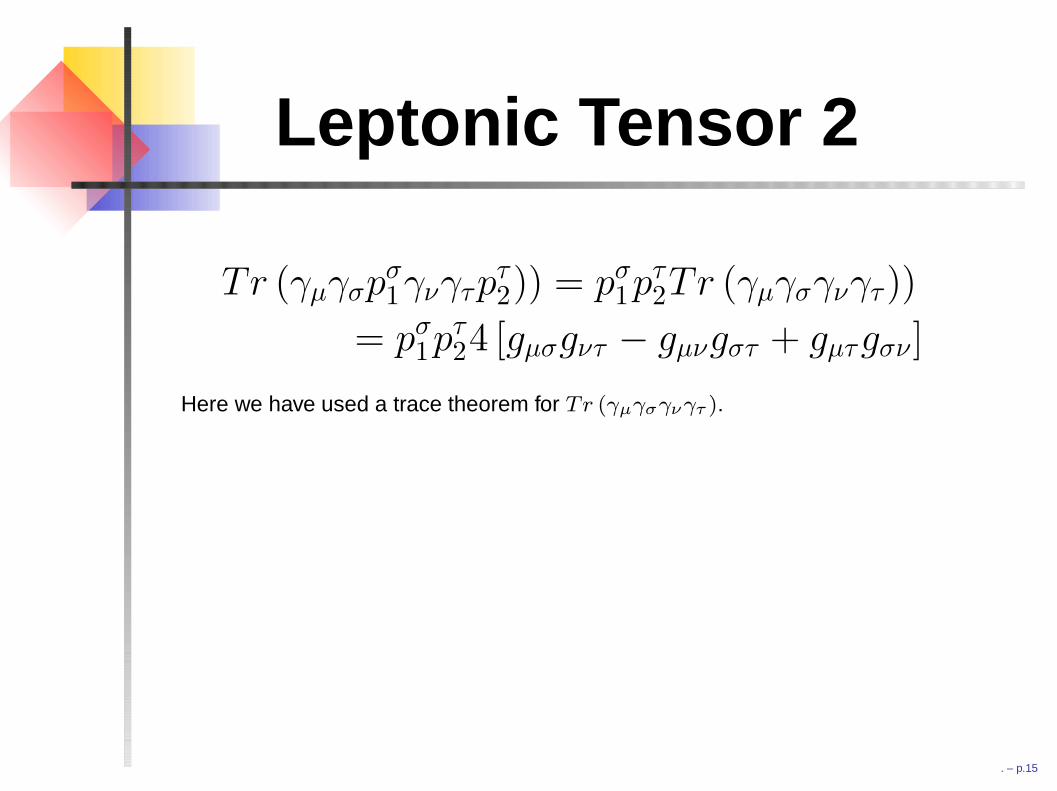
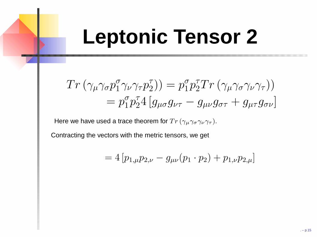
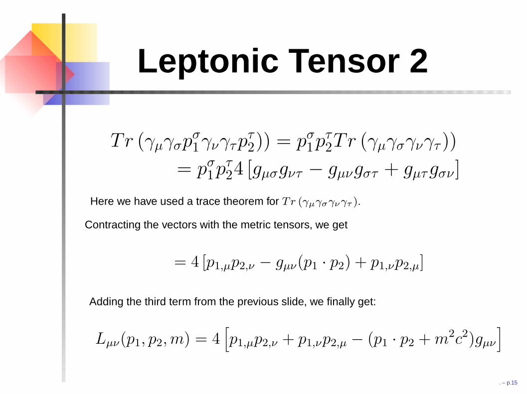
Tr (γµγσpσ1γνγτp
τ2)) = pσ
1pτ2Tr (γµγσγνγτ))
= pσ1p
τ24 [gµσgντ − gµνgστ + gµτgσν ]
Here we have used a trace theorem for Tr (γµγσγνγτ ).
Contracting the vectors with the metric tensors, we get
= 4 [p1,µp2,ν − gµν(p1 · p2) + p1,νp2,µ]
Adding the third term from the previous slide, we finally get:
Lµν(p1, p2,m) = 4[p1,µp2,ν + p1,νp2,µ − (p1 · p2 + m2c2)gµν
]
. – p.15
Leptonic Tensor 2
Tr (γµγσpσ1γνγτp
τ2)) = pσ
1pτ2Tr (γµγσγνγτ))
= pσ1p
τ24 [gµσgντ − gµνgστ + gµτgσν ]
Here we have used a trace theorem for Tr (γµγσγνγτ ).
Contracting the vectors with the metric tensors, we get
= 4 [p1,µp2,ν − gµν(p1 · p2) + p1,νp2,µ]
Adding the third term from the previous slide, we finally get:
Lµν(p1, p2,m) = 4[p1,µp2,ν + p1,νp2,µ − (p1 · p2 + m2c2)gµν
]
. – p.15

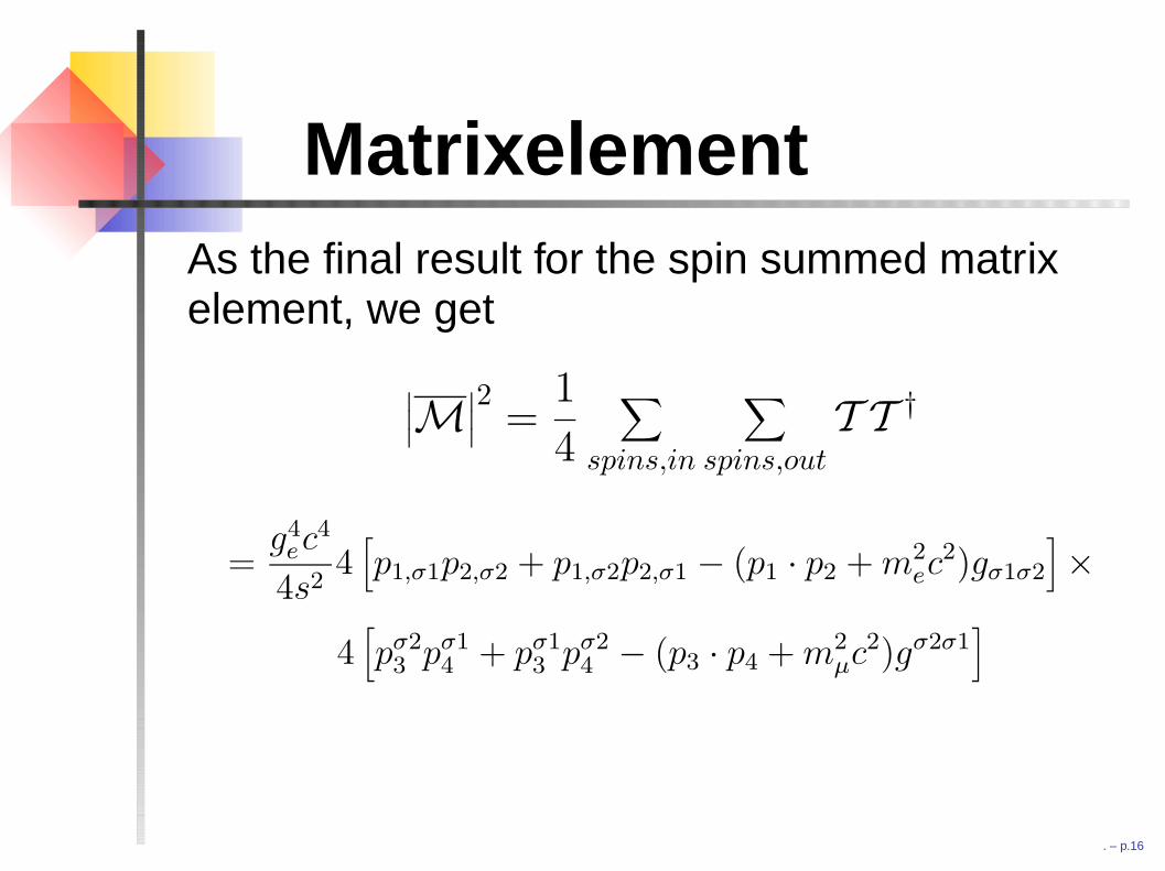
MatrixelementAs the final result for the spin summed matrixelement, we get
∣∣∣M∣∣∣2
=1
4
∑
spins,in
∑
spins,out
T T †
=g4
ec4
4s24
[p1,σ1p2,σ2 + p1,σ2p2,σ1 − (p1 · p2 + m2
ec2)gσ1σ2
]×
4[pσ2
3 pσ14 + pσ1
3 pσ24 − (p3 · p4 + m2
µc2)gσ2σ1
]
. – p.16
MatrixelementAs the final result for the spin summed matrixelement, we get
∣∣∣M∣∣∣2
=1
4
∑
spins,in
∑
spins,out
T T †
=g4
ec4
4s24
[p1,σ1p2,σ2 + p1,σ2p2,σ1 − (p1 · p2 + m2
ec2)gσ1σ2
]×
4[pσ2
3 pσ14 + pσ1
3 pσ24 − (p3 · p4 + m2
µc2)gσ2σ1
]
. – p.16

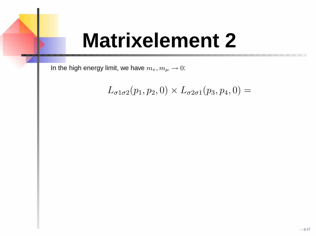
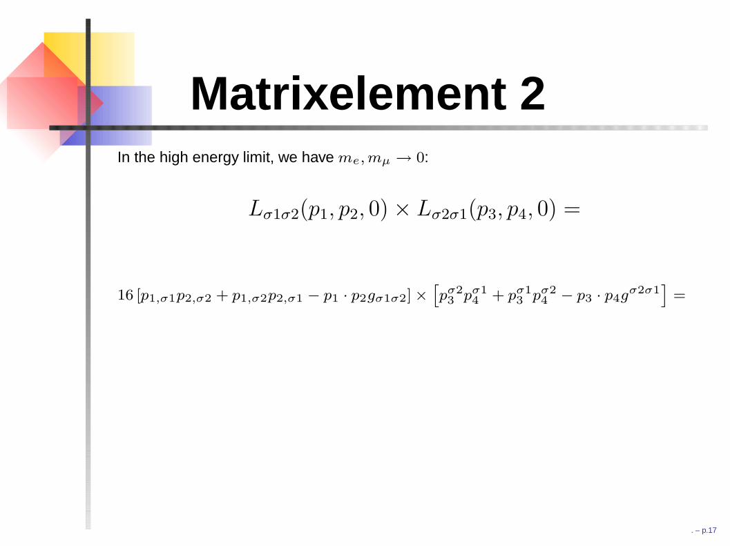
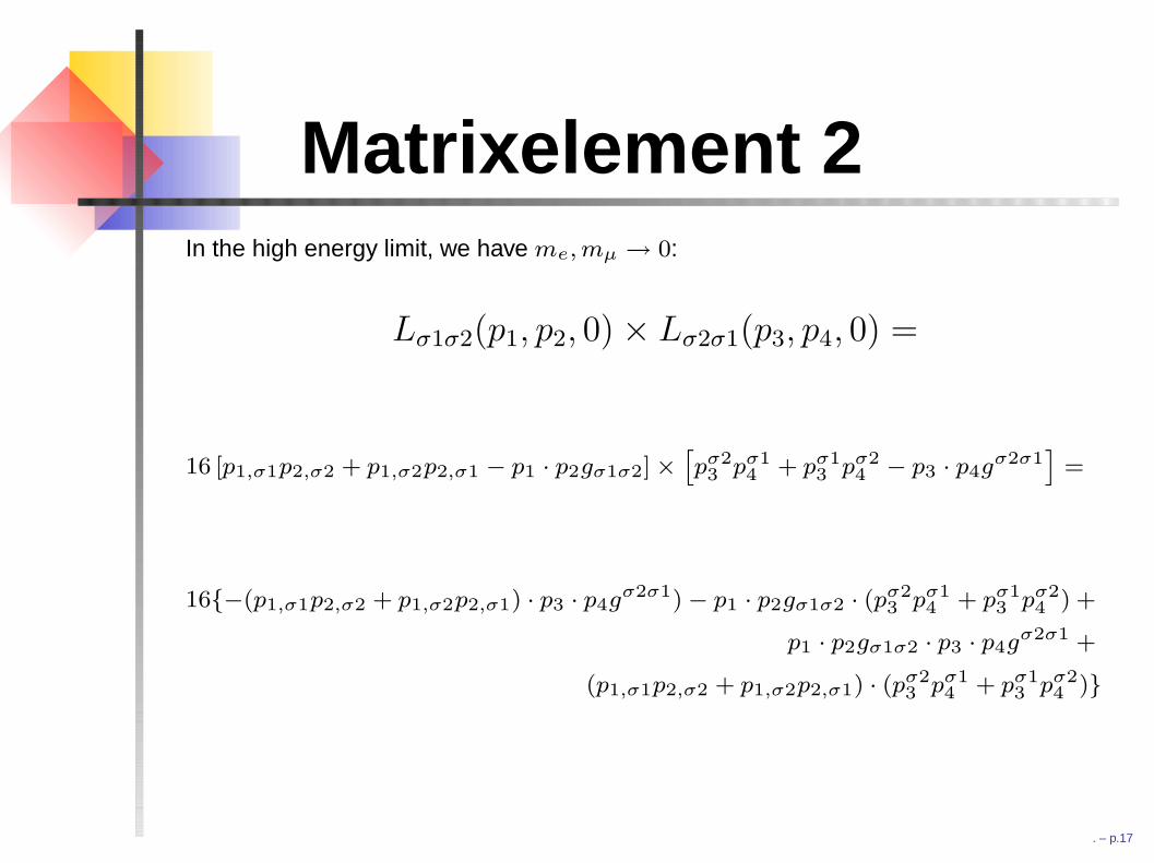
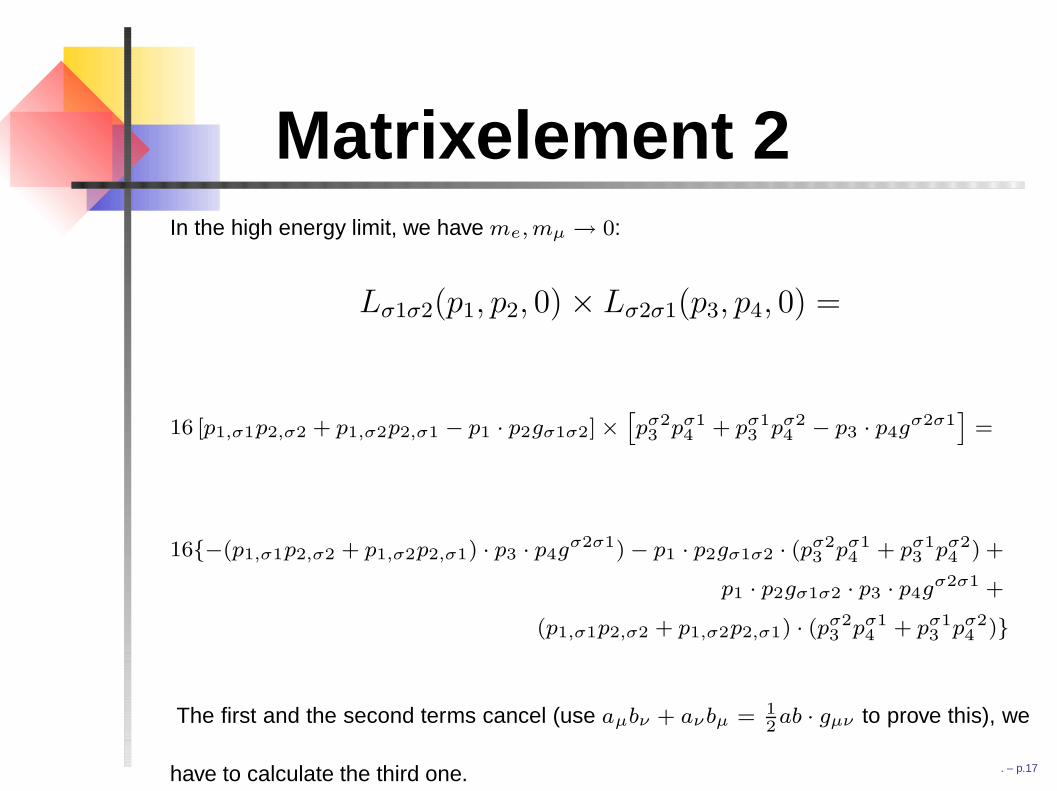
Matrixelement 2In the high energy limit, we have me, mµ → 0:
Lσ1σ2(p1, p2, 0)× Lσ2σ1(p3, p4, 0) =
16 [p1,σ1p2,σ2 + p1,σ2p2,σ1 − p1 · p2gσ1σ2]×[pσ23 pσ1
4 + pσ13 pσ2
4 − p3 · p4gσ2σ1]
=
16−(p1,σ1p2,σ2 + p1,σ2p2,σ1) · p3 · p4gσ2σ1)− p1 · p2gσ1σ2 · (pσ23 pσ1
4 + pσ13 pσ2
4 ) +
p1 · p2gσ1σ2 · p3 · p4gσ2σ1 +
(p1,σ1p2,σ2 + p1,σ2p2,σ1) · (pσ23 pσ1
4 + pσ13 pσ2
4 )
The first and the second terms cancel (use aµbν + aνbµ = 12ab · gµν to prove this), we
have to calculate the third one.
. – p.17
Matrixelement 2In the high energy limit, we have me, mµ → 0:
Lσ1σ2(p1, p2, 0)× Lσ2σ1(p3, p4, 0) =
16 [p1,σ1p2,σ2 + p1,σ2p2,σ1 − p1 · p2gσ1σ2]×[pσ23 pσ1
4 + pσ13 pσ2
4 − p3 · p4gσ2σ1]
=
16−(p1,σ1p2,σ2 + p1,σ2p2,σ1) · p3 · p4gσ2σ1)− p1 · p2gσ1σ2 · (p
σ23 pσ1
4 + pσ13 pσ2
4 ) +
p1 · p2gσ1σ2 · p3 · p4gσ2σ1 +
(p1,σ1p2,σ2 + p1,σ2p2,σ1) · (pσ23 pσ1
4 + pσ13 pσ2
4 )
The first and the second terms cancel (use aµbν + aνbµ = 12ab · gµν to prove this), we
have to calculate the third one.
. – p.17
Matrixelement 2In the high energy limit, we have me, mµ → 0:
Lσ1σ2(p1, p2, 0)× Lσ2σ1(p3, p4, 0) =
16 [p1,σ1p2,σ2 + p1,σ2p2,σ1 − p1 · p2gσ1σ2]×[pσ23 pσ1
4 + pσ13 pσ2
4 − p3 · p4gσ2σ1]
=
16−(p1,σ1p2,σ2 + p1,σ2p2,σ1) · p3 · p4gσ2σ1)− p1 · p2gσ1σ2 · (pσ23 pσ1
4 + pσ13 pσ2
4 ) +
p1 · p2gσ1σ2 · p3 · p4gσ2σ1 +
(p1,σ1p2,σ2 + p1,σ2p2,σ1) · (pσ23 pσ1
4 + pσ13 pσ2
4 )
The first and the second terms cancel (use aµbν + aνbµ = 12ab · gµν to prove this), we
have to calculate the third one.
. – p.17
Matrixelement 2In the high energy limit, we have me, mµ → 0:
Lσ1σ2(p1, p2, 0)× Lσ2σ1(p3, p4, 0) =
16 [p1,σ1p2,σ2 + p1,σ2p2,σ1 − p1 · p2gσ1σ2]×[pσ23 pσ1
4 + pσ13 pσ2
4 − p3 · p4gσ2σ1]
=
16−(p1,σ1p2,σ2 + p1,σ2p2,σ1) · p3 · p4gσ2σ1)− p1 · p2gσ1σ2 · (pσ23 pσ1
4 + pσ13 pσ2
4 ) +
p1 · p2gσ1σ2 · p3 · p4gσ2σ1 +
(p1,σ1p2,σ2 + p1,σ2p2,σ1) · (pσ23 pσ1
4 + pσ13 pσ2
4 )
The first and the second terms cancel (use aµbν + aνbµ = 12ab · gµν to prove this), we
have to calculate the third one. . – p.17
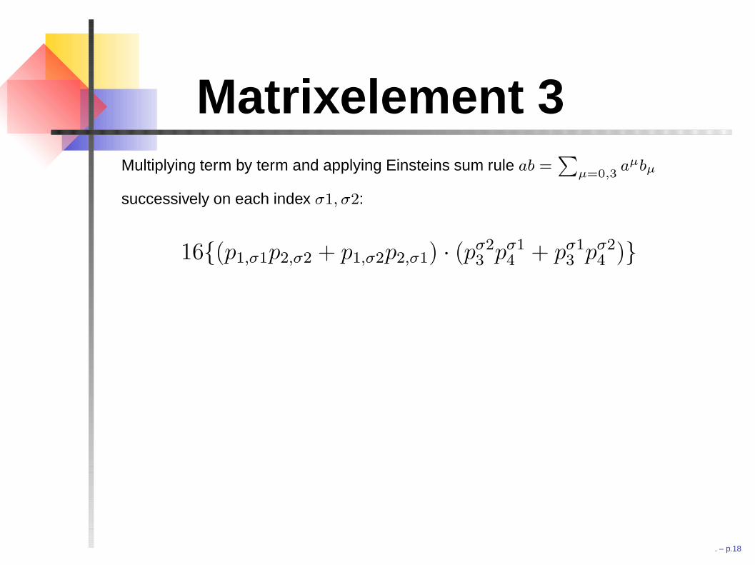
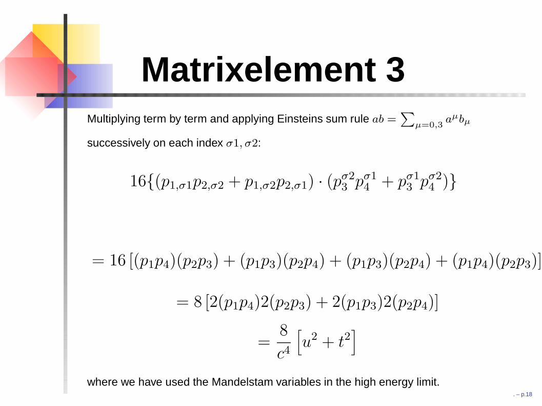
Matrixelement 3Multiplying term by term and applying Einsteins sum rule ab =
∑µ=0,3
aµbµ
successively on each index σ1, σ2:
16(p1,σ1p2,σ2 + p1,σ2p2,σ1) · (pσ23 pσ1
4 + pσ13 pσ2
4 )
= 16 [(p1p4)(p2p3) + (p1p3)(p2p4) + (p1p3)(p2p4) + (p1p4)(p2p3)]
= 8 [2(p1p4)2(p2p3) + 2(p1p3)2(p2p4)]
=8
c4
[u2 + t2
]
where we have used the Mandelstam variables in the high energy limit.
. – p.18
Matrixelement 3Multiplying term by term and applying Einsteins sum rule ab =
∑µ=0,3
aµbµ
successively on each index σ1, σ2:
16(p1,σ1p2,σ2 + p1,σ2p2,σ1) · (pσ23 pσ1
4 + pσ13 pσ2
4 )
= 16 [(p1p4)(p2p3) + (p1p3)(p2p4) + (p1p3)(p2p4) + (p1p4)(p2p3)]
= 8 [2(p1p4)2(p2p3) + 2(p1p3)2(p2p4)]
=8
c4
[u2 + t2
]
where we have used the Mandelstam variables in the high energy limit.. – p.18
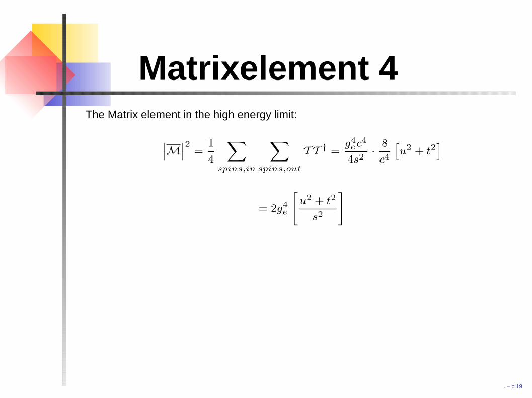
Matrixelement 4The Matrix element in the high energy limit:
∣∣M∣∣2 =
1
4
∑
spins,in
∑
spins,out
T T † =g4
ec4
4s2· 8
c4
[u2 + t2
]
= 2g4e
[u2 + t2
s2
]
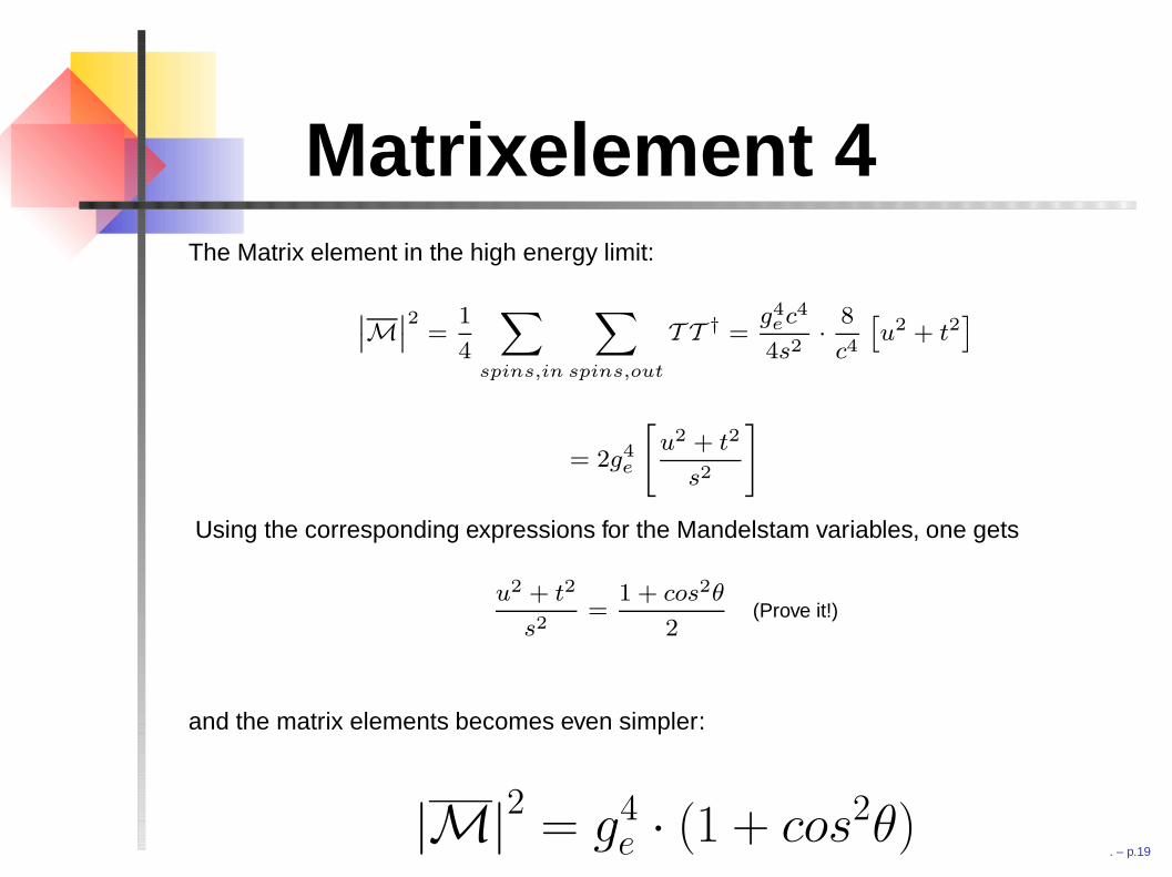
Using the corresponding expressions for the Mandelstam variables, one gets
u2 + t2
s2=
1 + cos2θ
2(Prove it!)
and the matrix elements becomes even simpler:
|M|2
= g4e · (1 + cos2θ)
. – p.19
Matrixelement 4The Matrix element in the high energy limit:
∣∣M∣∣2 =
1
4
∑
spins,in
∑
spins,out
T T † =g4
ec4
4s2· 8
c4
[u2 + t2
]
= 2g4e
[u2 + t2
s2
]
Using the corresponding expressions for the Mandelstam variables, one gets
u2 + t2
s2=
1 + cos2θ
2(Prove it!)
and the matrix elements becomes even simpler:
|M|2
= g4e · (1 + cos2θ)
. – p.19
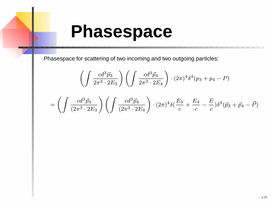
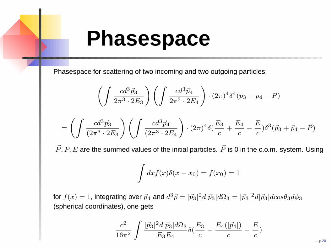
PhasespacePhasespace for scattering of two incoming and two outgoing particles:
(∫cd3~p3
2π3 · 2E3
)(∫cd3~p4
2π3 · 2E4
)· (2π)4δ4(p3 + p4 − P )
=
(∫cd3~p3
(2π3 · 2E3
)(∫cd3~p4
(2π3 · 2E4
)· (2π)4δ(
E3
c+
E4
c− E
c)δ3(~p3 + ~p4 − ~P )
~P , P, E are the summed values of the initial particles. ~P is 0 in the c.o.m. system. Using
∫dxf(x)δ(x− x0) = f(x0) = 1
for f(x) = 1, integrating over ~p4 and d3~p = |~p3|2d|~p3|dΩ3 = |~p3|2d|~p3|dcosθ3dφ3
(spherical coordinates), one gets
c2
16π2
∫|~p3|2d|~p3|dΩ3
E3E4δ(
E3
c+
E4(|~p4|)c
− E
c)
. – p.20
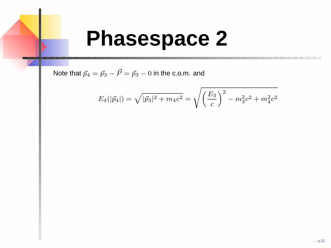
Phasespace 2
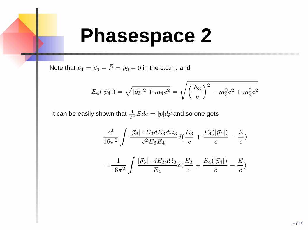
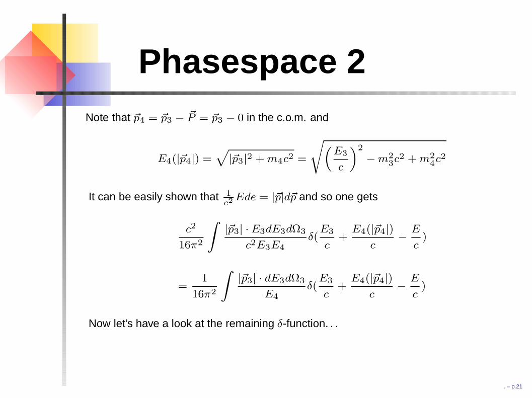
Note that ~p4 = ~p3 − ~P = ~p3 − 0 in the c.o.m. and
E4(|~p4|) =√|~p3|2 + m4c2 =
√(E3
c
)2
−m23c2 + m2
4c2
It can be easily shown that 1c2
Ede = |~p|d~p and so one gets
c2
16π2
∫|~p3| ·E3dE3dΩ3
c2E3E4δ(
E3
c+
E4(|~p4|)c
− E
c)
=1
16π2
∫|~p3| · dE3dΩ3
E4δ(
E3
c+
E4(|~p4|)c
− E
c)
Now let’s have a look at the remaining δ-
function. . .
. – p.21
Phasespace 2Note that ~p4 = ~p3 − ~P = ~p3 − 0 in the c.o.m. and
E4(|~p4|) =√|~p3|2 + m4c2 =
√(E3
c
)2
−m23c2 + m2
4c2
It can be easily shown that 1c2
Ede = |~p|d~p and so one gets
c2
16π2
∫|~p3| ·E3dE3dΩ3
c2E3E4δ(
E3
c+
E4(|~p4|)c
− E
c)
=1
16π2
∫|~p3| · dE3dΩ3
E4δ(
E3
c+
E4(|~p4|)c
− E
c)
Now let’s have a look at the remaining δ-function. . .
. – p.21
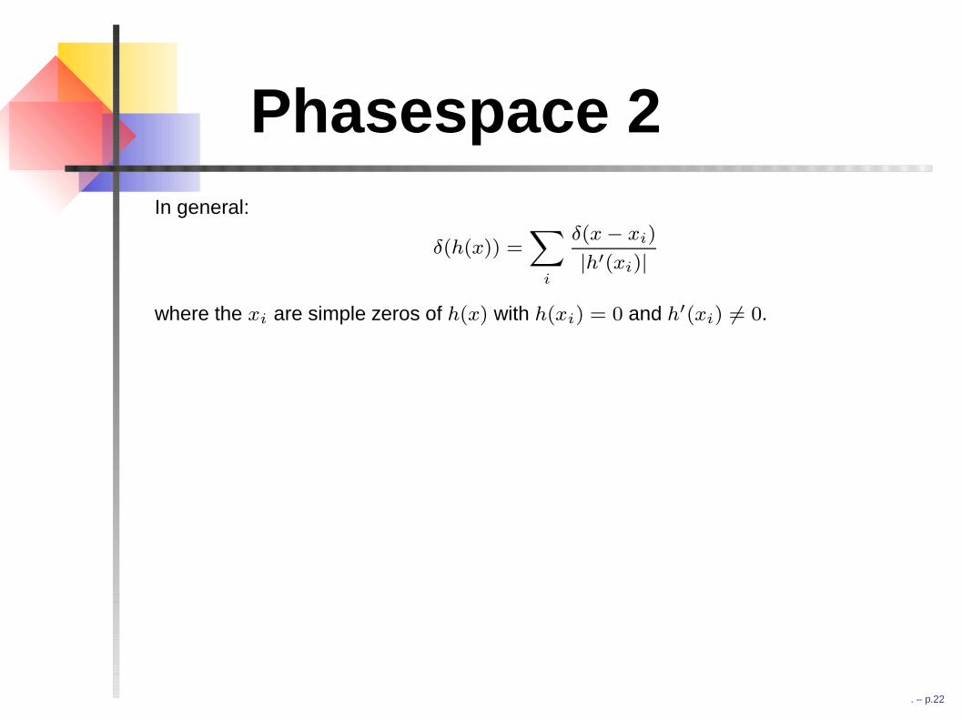
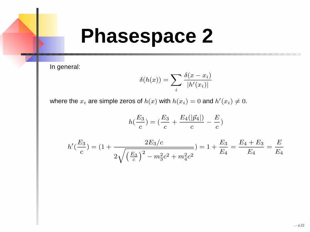
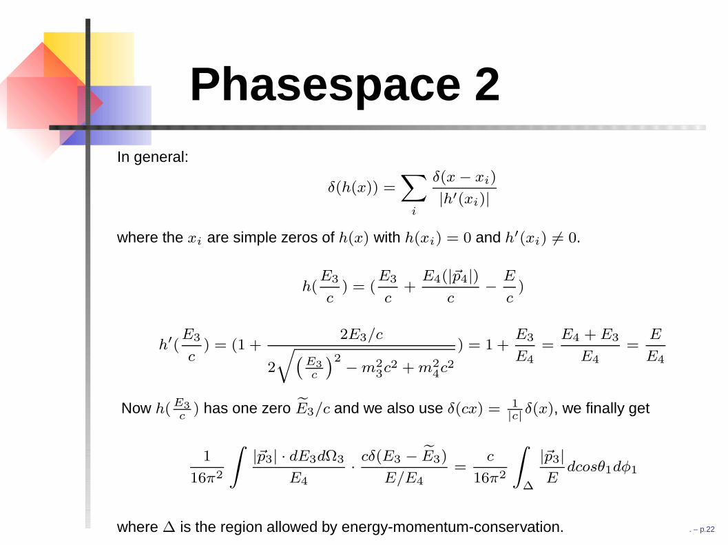
Phasespace 2In general:
δ(h(x)) =∑
i
δ(x− xi)
|h′(xi)|
where the xi are simple zeros of h(x) with h(xi) = 0 and h′(xi) 6= 0.
h(E3
c) = (
E3
c+
E4(|~p4|)c
− E
c)
h′(E3
c) = (1 +
2E3/c
2
√(E3
c
)2 −m23c2 + m2
4c2) = 1 +
E3
E4=
E4 + E3
E4=
E
E4
Now h( E3
c) has one zero E3/c and we also use δ(cx) = 1
|c|δ(x), we finally get
1
16π2
∫|~p3| · dE3dΩ3
E4· cδ(E3 − E3)
E/E4=
c
16π2
∫
∆
|~p3|E
dcosθ1dφ1
where ∆ is the region allowed by energy-momentum-conservation.
. – p.22
Phasespace 2In general:
δ(h(x)) =∑
i
δ(x− xi)
|h′(xi)|
where the xi are simple zeros of h(x) with h(xi) = 0 and h′(xi) 6= 0.
h(E3
c) = (
E3
c+
E4(|~p4|)c
− E
c)
h′(E3
c) = (1 +
2E3/c
2
√(E3
c
)2 −m23c2 + m2
4c2) = 1 +
E3
E4=
E4 + E3
E4=
E
E4
Now h( E3
c) has one zero E3/c and we also use δ(cx) = 1
|c|δ(x), we finally get
1
16π2
∫|~p3| · dE3dΩ3
E4· cδ(E3 − E3)
E/E4=
c
16π2
∫
∆
|~p3|E
dcosθ1dφ1
where ∆ is the region allowed by energy-momentum-conservation. . – p.22
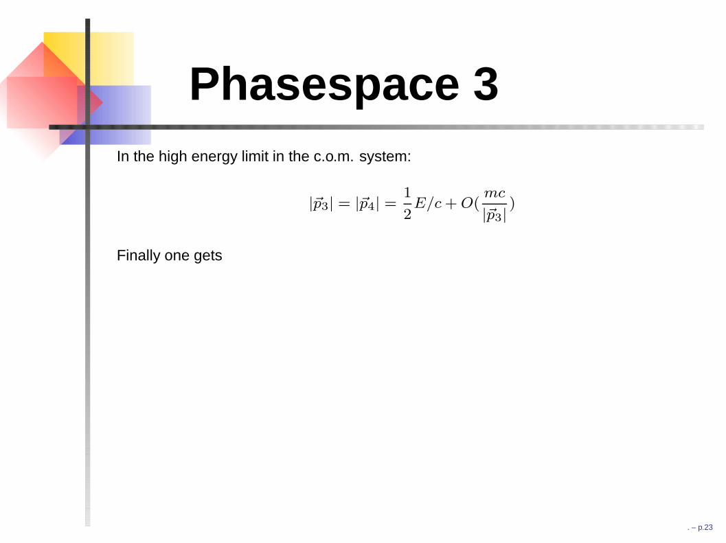
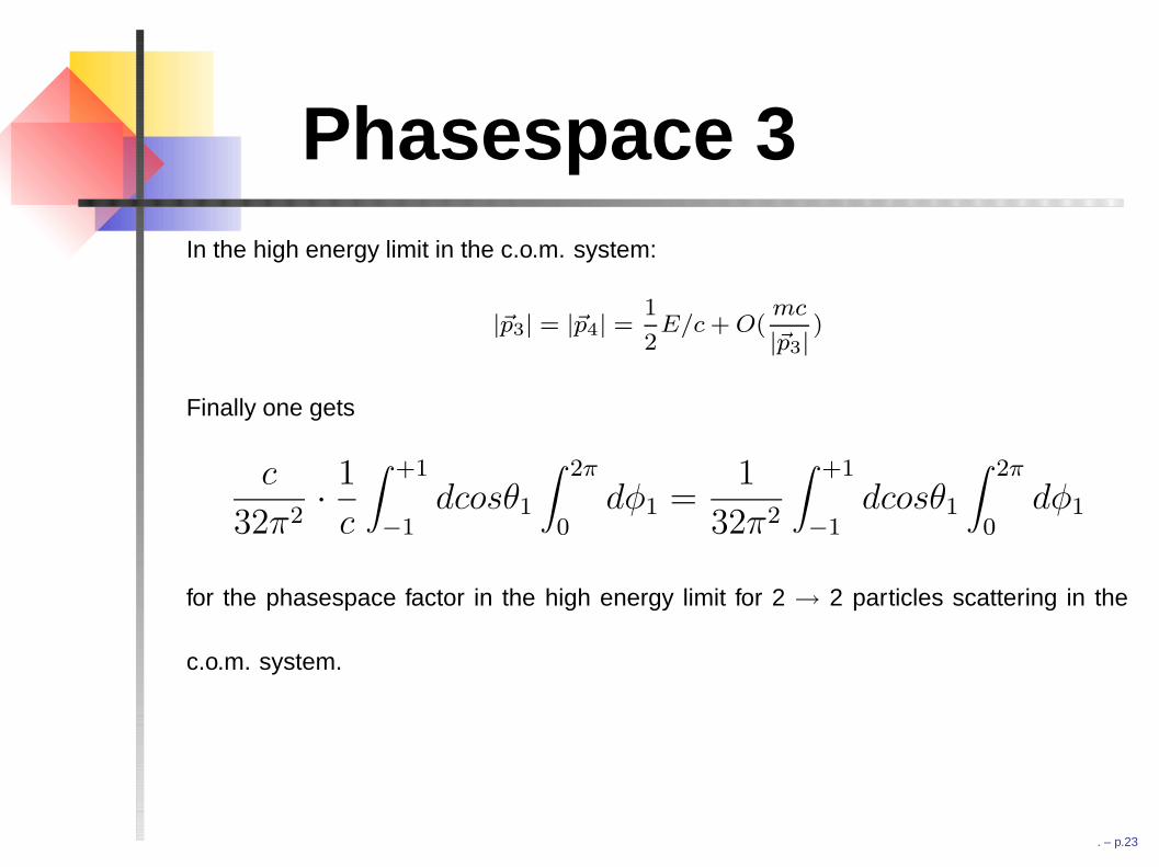
Phasespace 3In the high energy limit in the c.o.m. system:
|~p3| = |~p4| =1
2E/c + O(
mc
|~p3|)
Finally one gets
c
32π2·1
c
∫ +1
−1dcosθ1
∫ 2π
0dφ1 =
1
32π2
∫ +1
−1dcosθ1
∫ 2π
0dφ1
for the phasespace factor in the high energy limit for 2 → 2 particles scattering in the
c.o.m. system.
. – p.23
Phasespace 3In the high energy limit in the c.o.m. system:
|~p3| = |~p4| =1
2E/c + O(
mc
|~p3|)
Finally one gets
c
32π2·1
c
∫ +1
−1dcosθ1
∫ 2π
0dφ1 =
1
32π2
∫ +1
−1dcosθ1
∫ 2π
0dφ1
for the phasespace factor in the high energy limit for 2 → 2 particles scattering in the
c.o.m. system.
. – p.23
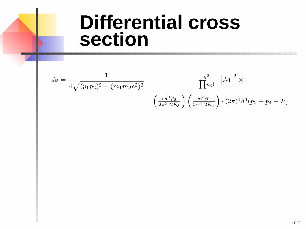
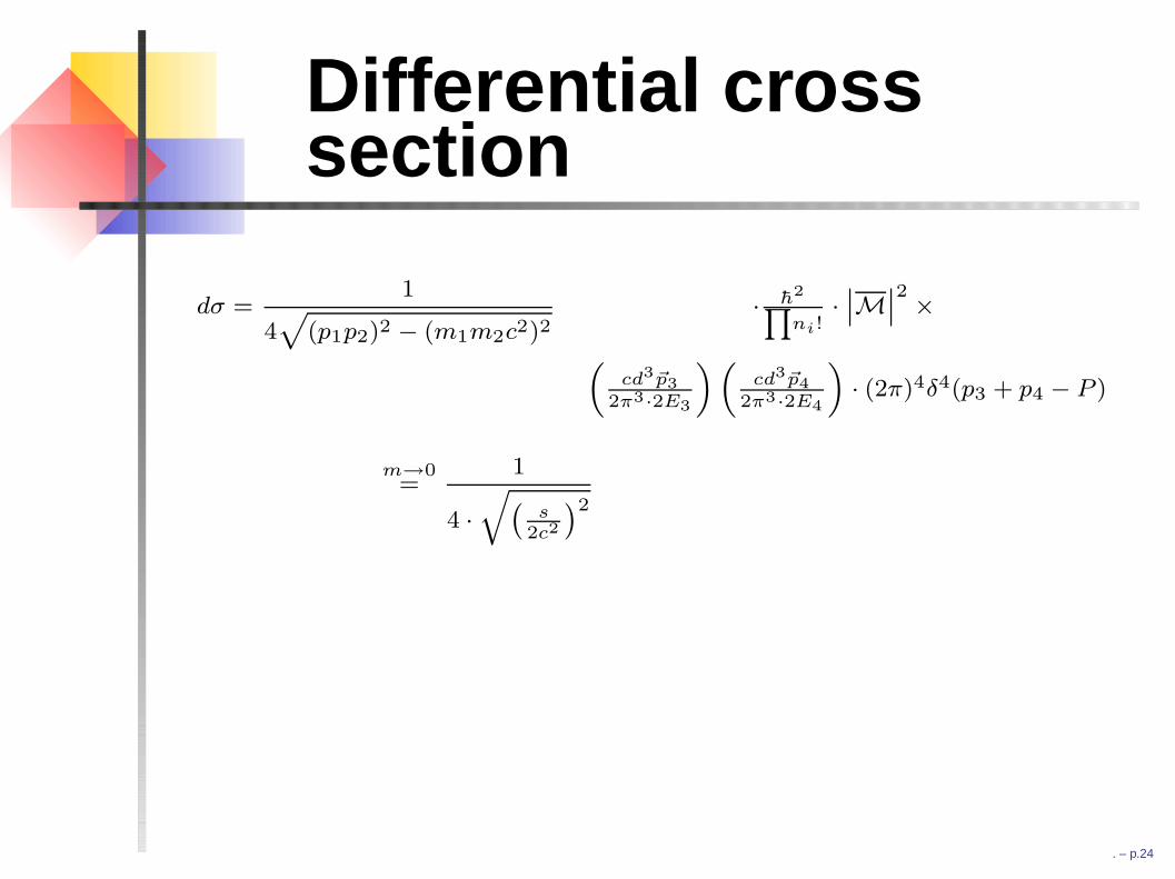
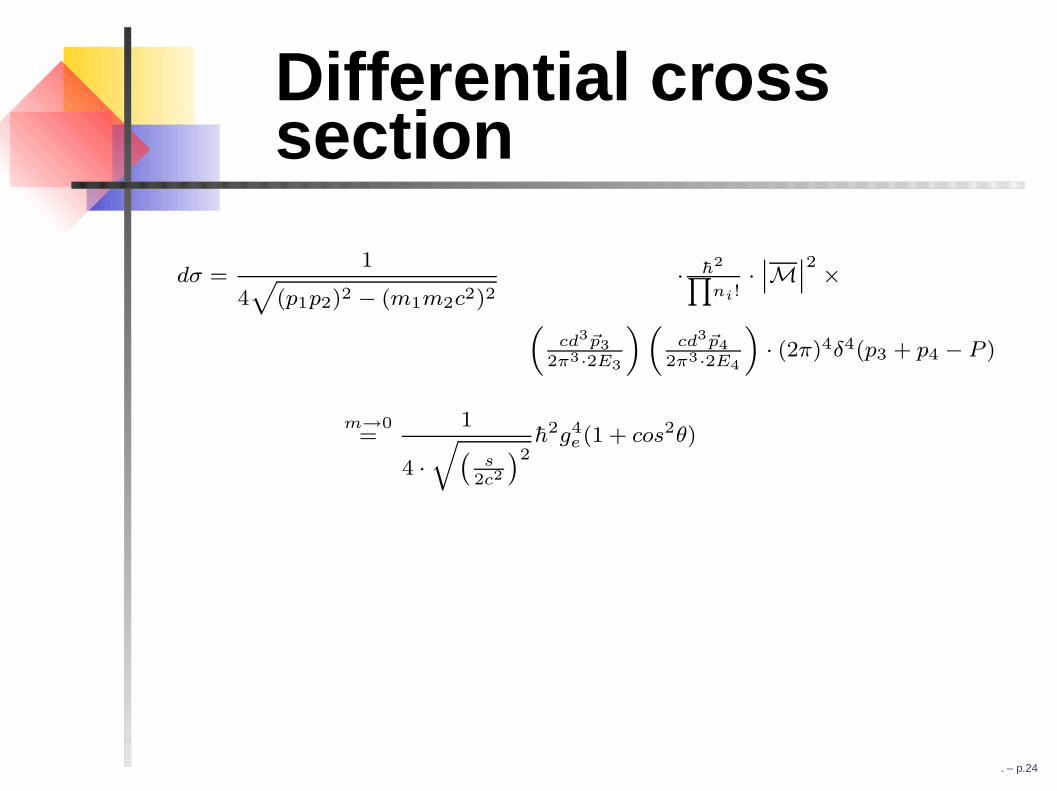
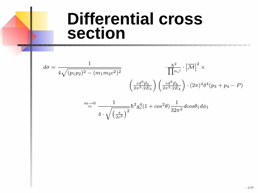
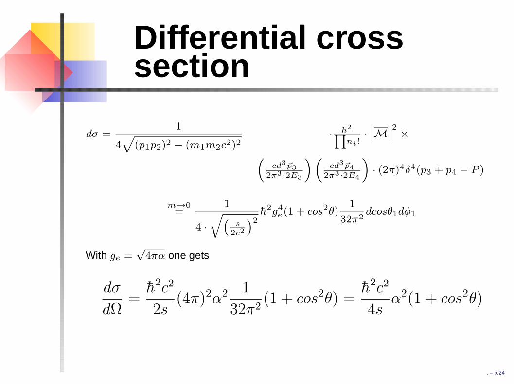
Differential crosssection
dσ =1
4√
(p1p2)2 − (m1m2c2)2· h2∏
ni!·∣∣M
∣∣2 ×(
cd3~p3
2π3·2E3
)(cd3~p4
2π3·2E4
)· (2π)4δ4(p3 + p4 − P )
m→0=
1
4 ·√(
s2c2
)2h2g4
e(1 + cos2θ)1
32π2dcosθ1dφ1
With ge =√
4πα one gets
dσ
dΩ=
h2c2
2s(4π)2α2 1
32π2(1 + cos2θ) =
h2c2
4sα2(1 + cos2θ)
. – p.24
Differential crosssection
dσ =1
4√
(p1p2)2 − (m1m2c2)2· h2∏
ni!·∣∣M
∣∣2 ×(
cd3~p3
2π3·2E3
)(cd3~p4
2π3·2E4
)· (2π)4δ4(p3 + p4 − P )
m→0=
1
4 ·√(
s2c2
)2
h2g4e(1 + cos2θ)
1
32π2dcosθ1dφ1
With ge =√
4πα one gets
dσ
dΩ=
h2c2
2s(4π)2α2 1
32π2(1 + cos2θ) =
h2c2
4sα2(1 + cos2θ)
. – p.24

Differential crosssection
dσ =1
4√
(p1p2)2 − (m1m2c2)2· h2∏
ni!·∣∣M
∣∣2 ×(
cd3~p3
2π3·2E3
)(cd3~p4
2π3·2E4
)· (2π)4δ4(p3 + p4 − P )
m→0=
1
4 ·√(
s2c2
)2h2
g4e(1 + cos2θ)
1
32π2dcosθ1dφ1
With ge =√
4πα one gets
dσ
dΩ=
h2c2
2s(4π)2α2 1
32π2(1 + cos2θ) =
h2c2
4sα2(1 + cos2θ)
. – p.24
Differential crosssection
dσ =1
4√
(p1p2)2 − (m1m2c2)2· h2∏
ni!·∣∣M
∣∣2 ×(
cd3~p3
2π3·2E3
)(cd3~p4
2π3·2E4
)· (2π)4δ4(p3 + p4 − P )
m→0=
1
4 ·√(
s2c2
)2h2g4
e(1 + cos2θ)
1
32π2dcosθ1dφ1
With ge =√
4πα one gets
dσ
dΩ=
h2c2
2s(4π)2α2 1
32π2(1 + cos2θ) =
h2c2
4sα2(1 + cos2θ)
. – p.24
Differential crosssection
dσ =1
4√
(p1p2)2 − (m1m2c2)2· h2∏
ni!·∣∣M
∣∣2 ×(
cd3~p3
2π3·2E3
)(cd3~p4
2π3·2E4
)· (2π)4δ4(p3 + p4 − P )
m→0=
1
4 ·√(
s2c2
)2h2g4
e(1 + cos2θ)1
32π2dcosθ1dφ1
With ge =√
4πα one gets
dσ
dΩ=
h2c2
2s(4π)2α2 1
32π2(1 + cos2θ) =
h2c2
4sα2(1 + cos2θ)
. – p.24
Differential crosssection
dσ =1
4√
(p1p2)2 − (m1m2c2)2· h2∏
ni!·∣∣M
∣∣2 ×(
cd3~p3
2π3·2E3
)(cd3~p4
2π3·2E4
)· (2π)4δ4(p3 + p4 − P )
m→0=
1
4 ·√(
s2c2
)2h2g4
e(1 + cos2θ)1
32π2dcosθ1dφ1
With ge =√
4πα one gets
dσ
dΩ=
h2c2
2s(4π)2α2 1
32π2(1 + cos2θ) =
h2c2
4sα2(1 + cos2θ)
. – p.24
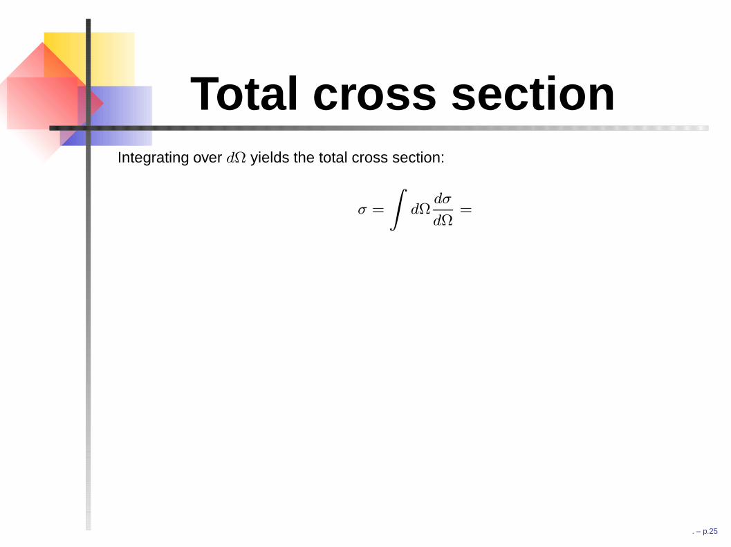
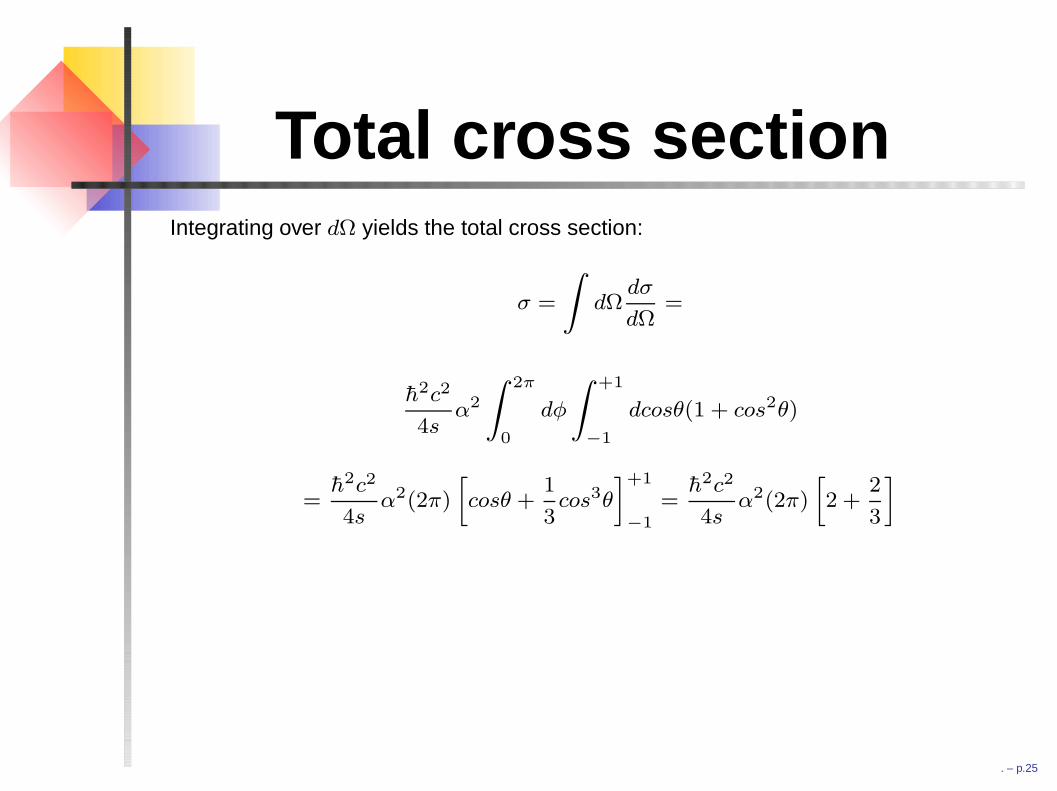
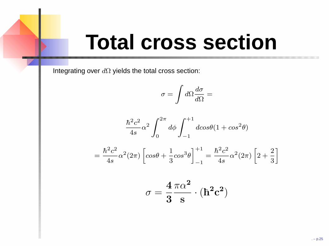
Total cross sectionIntegrating over dΩ yields the total cross section:
σ =
∫dΩ
dσ
dΩ=
h2c2
4sα2
∫ 2π
0
dφ
∫ +1
−1
dcosθ(1 + cos2θ)
=h2c2
4sα2(2π)
[cosθ +
1
3cos3θ
]+1
−1=
h2c2
4sα2(2π)
[2 +
2
3
]
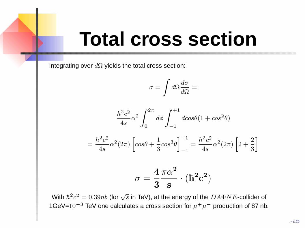
σ =4
3
πα2
s· (h2
c2)
With h2c2 = 0.39nb (for√
s in TeV), at the energy of the DAΦNE-collider of1GeV=10−3 TeV one calculates a cross section for µ+µ− production of 87 nb.
. – p.25

Total cross sectionIntegrating over dΩ yields the total cross section:
σ =
∫dΩ
dσ
dΩ=
h2c2
4sα2
∫ 2π
0
dφ
∫ +1
−1
dcosθ(1 + cos2θ)
=h2c2
4sα2(2π)
[cosθ +
1
3cos3θ
]+1
−1=
h2c2
4sα2(2π)
[2 +
2
3
]
σ =4
3
πα2
s· (h2
c2)
With h2c2 = 0.39nb (for√
s in TeV), at the energy of the DAΦNE-collider of1GeV=10−3 TeV one calculates a cross section for µ+µ− production of 87 nb.
. – p.25
Total cross sectionIntegrating over dΩ yields the total cross section:
σ =
∫dΩ
dσ
dΩ=
h2c2
4sα2
∫ 2π
0
dφ
∫ +1
−1
dcosθ(1 + cos2θ)
=h2c2
4sα2(2π)
[cosθ +
1
3cos3θ
]+1
−1=
h2c2
4sα2(2π)
[2 +
2
3
]
σ =4
3
πα2
s· (h2
c2)
With h2c2 = 0.39nb (for√
s in TeV), at the energy of the DAΦNE-collider of
1GeV=10−3 TeV one calculates a cross section for µ+µ− production of 87 nb.
. – p.25
Total cross sectionIntegrating over dΩ yields the total cross section:
σ =
∫dΩ
dσ
dΩ=
h2c2
4sα2
∫ 2π
0
dφ
∫ +1
−1
dcosθ(1 + cos2θ)
=h2c2
4sα2(2π)
[cosθ +
1
3cos3θ
]+1
−1=
h2c2
4sα2(2π)
[2 +
2
3
]
σ =4
3
πα2
s· (h2
c2)
With h2c2 = 0.39nb (for√
s in TeV), at the energy of the DAΦNE-collider of1GeV=10−3 TeV one calculates a cross section for µ+µ− production of 87 nb.
. – p.25