Discrete Fourier Transform and Fast Fourier Transform 1

The discrete Fourier transform (DFT) has several practical applications including:

• signal processing

• partial differential equations

• polynomial multiplication and interpolation

A simple practical example: Consider the Fourier series representation of a continuous periodic functionon the interval [0 2π]:

f(x) = a0 +∞∑

k=1

(ak cos kx + bk sin kx)

Using the Euler’s formulas

cos θ =eiθ + e−iθ

2, sin θ =

eiθ − e−iθ

2i

the complex form of the Fourier series may be written

f(x) =∞∑

k=−∞

cke−ikx

where

c0 = a0, ck =ak + ibk

2(1)

The complex Fourier coefficients are given by the formula:

ck =1

2π

∫ 2π

0

f(x)eikx dx (2)

and if f is a real-valued function then c−k = ck. Once the complex coefficients are found, ak and bk maybe recovered from (1).

If numerical integration with the nodes h = 2π/n, xj = 2jπ/n, j = 0, 1, . . . n is used to evaluate (2)the approximation formula become:

ck =1

n

n−1∑j=0

f(xj)eikxj =

1

n

n−1∑j=0

f(xj)e2πikj/n =

1

n

n−1∑j=0

f(xj)(e2πi/n

)kj, k = 0, 1, . . . (3)

Definition: Given a vector a = (a0, a1, . . . , an−1) we define the Discrete Fourier Transform of a as thevector y = (y0, y1, . . . , yn−1) whose components are

ydef= DFTn(a); yk =

n−1∑j=0

ajωkjn , k = 0, 1, . . . , n− 1 (4)

1Reference: ”Introduction to Algorithms” by T.H. Cormen, C.E. Leiserson and R.L. Rivest. MIT Press, 1990.

1

where ωn is the principal nth root of the unity

ωn = e2πi/n

All other complex roots of order n of the unity are powers of ωn

ω0n, ω

1n, . . . , ω

n−1n

The problem of evaluating DFT (a) is equivalent to the problem of evaluating the polynomial

A(x) =n−1∑j=0

ajxj (5)

at the complex roots of order n of the unity, since

yk = A(ωkn), k = 0, 1, . . . n− 1

If we define the DFT matrix as

F ∈ Rn×n, Fk,j = ωkjn , 0 ≤ k, j ≤ n− 1 (6)

then y may be written as the matrix vector product

y = Fa (7)

For example, with n = 4 the DFT matrix is:

F4 =

1 1 1 11 ω4 ω2

4 ω34

1 ω24 ω4

4 ω64

1 ω34 ω6

4 ω94

=

1 1 1 11 i −1 −i1 −1 1 −11 −i −1 i

The inverse discrete Fourier transform (IDFT) is

DFT−1(y) = F−1y (8)

and one notices that IDFT solves the problem of interpolation at the roots of the unity:

Given the data points (ωkn, yk), k = 0, 1, . . . n− 1 find the polynomial of A(x) degree n− 1 such that

A(ωkn) = yk, k = 0, 1, . . . n− 1

Evaluating DFT (a) using standard multiplication has a computational complexity of order O(n2).

The Fast Fourier Transform (FFT, Cooley-Tukey 1965) provides an algorithm to evaluate DFT with acomputational complexity of order O(n log n) where log = log2. As we shall see shortly, IDFT may be thenevaluated as well using O(n log n) operations. The computational savings are significant. For example,if n = 103, the standard DFT requires ∼ 106 operations, whereas FFT will involve only ∼ 104, thus a

2

computational saving by a factor of 100.

In order to introduce FFT we first review some important properties of the roots of order n of the unity.

Lemma 1: For any integers n ≥ 0, k ≥ 0, and d > 0

ωdkdn = ωk

n (9)

Proof:

ωdkdn = e

2πidn

dk = e2πin

k = ωkn

Lemma 2: For any even integer n > 0ωn/2

n = −1 (10)

Proof: Let n = 2m, m > 0.

ωn/2n = e

2πi2m

m = eπi = −1

Lemma 3: If n > 0 is even, then(ωk

n)2 = ωkn/2 (11)

Proof:

(ωkn)2 = ω2k

n = ω2k2n/2

lemma1= ωk

n/2

Lemma 4: For any integer n ≥ 1 and any integer k > 0 such that k modn 6= 0

n−1∑j=0

(ωkn)j = 0 (12)

Proof:n−1∑j=0

(ωkn)j =

(ωkn)n − 1

ωkn − 1

=(ωn

n)k − 1

ωkn − 1

= 0

since k mod n 6= 0 ⇒ ωkn 6= 1.

Property: For any integers j, k ≥ 0,

ωjnω

kn = ω(j+k)mod n

n , ωkjn = ωkj mod n

n (13)

Lemma 5: The inverse of the DFT matrix is obtained by conjugating the entries of F and scaling by n:

F−1 =1

nF , F−1

k,j =1

nωkj

n , 0 ≤ k, j ≤ n− 1 (14)

whereωn = e−

2πin = ω−1

n

3

Proof: We show that F−1F = In, the identity matrix.

(F−1F )k,l =1

n

n−1∑j=0

ωkjn ωjl

n =1

n

n−1∑j=0

ω−kjn ωjl

n =1

n

n−1∑j=0

ω(l−k)jn =

1

n

n−1∑j=0

(ω(l−k)n )j = δk,l

where δk,l = 0, k 6= l and δl,l = 1. The last equality in the equation above follows from Lemma 4.

The FFT algorithm

The FFT algorithm takes advantage of the properties of the complex roots of the unity to calculateDFT(a) using O(n log n) operations. We assume that n is a power of 2, n = 2m (radix-2 algorithm). TheFFT method is a divide-and-conquer algorithm that recursively breaks a DFT of size n into two DFTs ofsize n/2 and an additional O(n) multiplications.

By separating the even-index and the odd-index coefficients, the polynomial (5) may be written

A(x) = A[0](x2) + xA[1](x2) (15)

where

A[0](x) = a0 + a2x + a4x2 + . . . + an−2x

n/2−1 (16)

A[1](x) = a1 + a3x + a5x2 + . . . + an−1x

n/2−1 (17)

are polynomials of degree n/2− 1.

The problem of evaluating A at ω0n, ω

1n, . . . , ω

n−1n is thus reduced to

1. Evaluate the polynomials A[0] and A[1] of degree n/2− 1 at (ω0n)2, (ω1

n)2, . . . , (ωn−1n )2

2. combine the results according to (15)

A fundamental remark is that (ω0n)2, (ω1

n)2, . . . , (ωn−1n )2 are not n distinct values, but, according to

Lemma 3, they are the n/2 complex roots of order n/2 of the unity. Therefore, each subproblem for A[0]

and A[1] has exactly the same form as the problem for A but are of half size. The original problem of sizen is thus decomposed into two problems each os size n/2 and an additional overhead (15) that requiresone multiplication and one addition for each value ω0

n, ω1n, . . . , ω

n−1n .

4

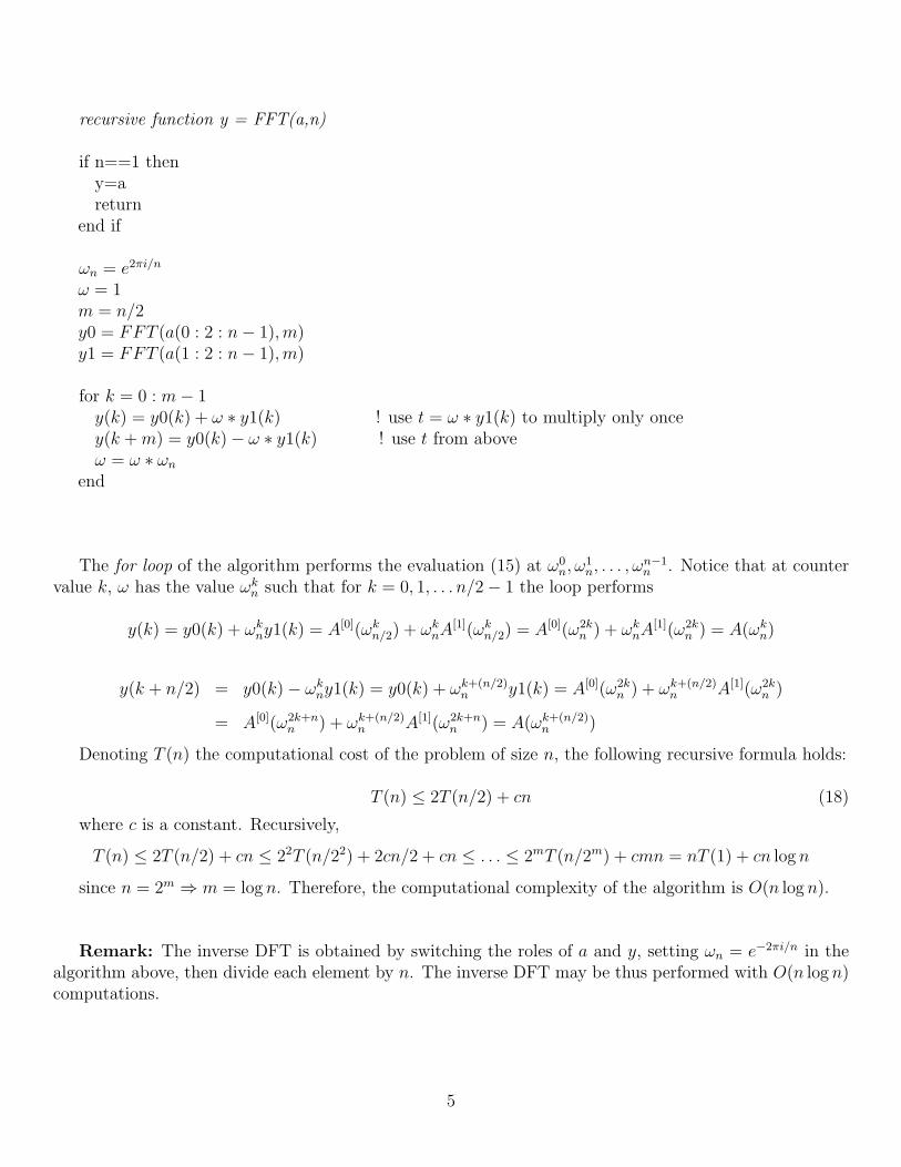
recursive function y = FFT(a,n)

if n==1 theny=areturn

end if

ωn = e2πi/n

ω = 1m = n/2y0 = FFT (a(0 : 2 : n− 1), m)y1 = FFT (a(1 : 2 : n− 1), m)

for k = 0 : m− 1y(k) = y0(k) + ω ∗ y1(k) ! use t = ω ∗ y1(k) to multiply only oncey(k + m) = y0(k)− ω ∗ y1(k) ! use t from aboveω = ω ∗ ωn

end

The for loop of the algorithm performs the evaluation (15) at ω0n, ω

1n, . . . , ω

n−1n . Notice that at counter

value k, ω has the value ωkn such that for k = 0, 1, . . . n/2− 1 the loop performs

y(k) = y0(k) + ωkny1(k) = A[0](ωk

n/2) + ωknA

[1](ωkn/2) = A[0](ω2k

n ) + ωknA

[1](ω2kn ) = A(ωk

n)

y(k + n/2) = y0(k)− ωkny1(k) = y0(k) + ωk+(n/2)

n y1(k) = A[0](ω2kn ) + ωk+(n/2)

n A[1](ω2kn )

= A[0](ω2k+nn ) + ωk+(n/2)

n A[1](ω2k+nn ) = A(ωk+(n/2)

n )

Denoting T (n) the computational cost of the problem of size n, the following recursive formula holds:

T (n) ≤ 2T (n/2) + cn (18)

where c is a constant. Recursively,

T (n) ≤ 2T (n/2) + cn ≤ 22T (n/22) + 2cn/2 + cn ≤ . . . ≤ 2mT (n/2m) + cmn = nT (1) + cn log n

since n = 2m ⇒ m = log n. Therefore, the computational complexity of the algorithm is O(n log n).

Remark: The inverse DFT is obtained by switching the roles of a and y, setting ωn = e−2πi/n in thealgorithm above, then divide each element by n. The inverse DFT may be thus performed with O(n log n)computations.

5

Data structure in the recursive calls

a0, a1, a2, a3, a4, a5, a6, a7

a1, a3, a5, a7

a0, a4 a2, a6 a1, a5 a3, a7

a0,a2,a4,a6

a0 a4 a2 a6 a1 a5 a3 a7

To get the elements of the input vector a into the desired order, a bit-reverse operation may be per-formed. In binary representation the bit-reverse operation results in

0 = 000 → 000 = 01 = 001 → 100 = 42 = 010 → 010 = 23 = 011 → 110 = 64 = 100 → 001 = 15 = 101 → 101 = 56 = 110 → 011 = 37 = 111 → 111 = 7such that if we bit-reverse-copy a into A, A[rev(k)] = a[k], then A will hold the elements of a in the desiredorder. This may be used to implement an iterative FFT algorithm

Iterative-FFT(a)

bit-reverse-copy(a, A)n = length(a)for s = 1 : log 2(n)

m = 2s

ωm = e2πi/m

ω = 1for j = 0 : m/2− 1

for k = j : m : n− 1t = ω ∗ A(k + m/2)u = A(k)A(k) = u + tA(k + m/2) = u− tω = ω ∗ ωm

return A

6

Two-dimensional Discrete Fourier Transform using Fast Fourier Transform

The 2D discrete Fourier transform is defined for a matrix a ∈ Cm×n.

Definition: Given a matrix a = (ai,j) ∈ Cm×n we define the 2D Discrete Fourier Transform of a as thematrix y = (yl,k) ∈ Cm×n whose entries are

ydef= DFT2(a), yl,k =

n−1∑j=0

m−1∑q=0

aq,jωlqmωjk

n , 0 ≤ l ≤ m− 1, 0 ≤ k ≤ n− 1 (19)

where ωm and ωn are the principal roots of the unity of order m and n, respectively:

ωm = e2πi/m, ωn = e2πi/n

If a standard approach is used, then evaluating DFT2(a) would require O(n2m2) operations. Using theproperties of DFT2 and one dimensional FFT the cost may be reduced to O(mn log(mn)) as we show next.

One notices that we may write (19) as

yl,k =n−1∑j=0

[m−1∑q=0

aq,jωlqm

]ωjk

n , 0 ≤ l ≤ m− 1, 0 ≤ k ≤ n− 1 (20)

For each fixed j in the range 0 ≤ j ≤ n − 1, the sum∑m−1

q=0 aq,jωlqm, 0 ≤ l ≤ m − 1 represents the one

dimensional DFT of the column j of the matrix a, a(:, j). Thus if we denote

y(:, j) = DFT (a(:, j)) ∈ Cm, y(l, j) =m−1∑q=0

aq,jωlqm, 0 ≤ l ≤ m− 1 (21)

then DFT2(a) may be obtained as

yl,k =n−1∑j=0

y(l, j)ωjkn , 0 ≤ l ≤ m− 1, 0 ≤ k ≤ n− 1 (22)

For each fixed l in the range 0 ≤ l ≤ m − 1 the computation (22) represents the 1D DFT of the datay(l, :) ∈ Cn.

The computation (21) is performed using n 1D FFTs for data of size m, at a computational costcost1 = nO(m log m). The computation of (22) is performed using an additional m 1D FFTs of data ofsize n, at a computational cost cost2 = mO(n log n). Overall,

cost = cost1 + cost2 = O(mn log mn)

7

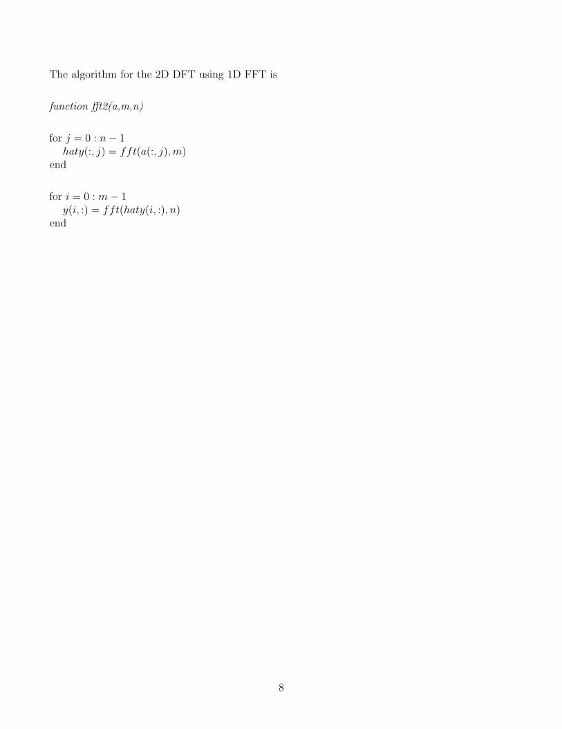
The algorithm for the 2D DFT using 1D FFT is

function fft2(a,m,n)

for j = 0 : n− 1haty(:, j) = fft(a(:, j), m)

end

for i = 0 : m− 1y(i, :) = fft(haty(i, :), n)

end

8