Dimensionality reduction via sparse matrices€¦ · Dimensionality reduction via sparse matrices...
80
Dimensionality reduction via sparse matrices Jelani Nelson Harvard September 19, 2013 based on works with Daniel Kane (Stanford) and Huy Nguy ˜ ˆ en (Princeton)
Transcript of Dimensionality reduction via sparse matrices€¦ · Dimensionality reduction via sparse matrices...

Dimensionality reduction via sparse matrices
Jelani NelsonHarvard
September 19, 2013
based on works with Daniel Kane (Stanford) and Huy Nguy˜en (Princeton)
Metric Johnson-Lindenstrauss lemma
Metric JL (MJL) Lemma, 1984
Every set of N points in Euclidean space can be embedded intoO(ε−2 logN)-dimensional Euclidean space so that all pairwisedistances are preserved up to a 1± ε factor.
Uses:
• Speed up geometric algorithms by first reducing dimension ofinput [Indyk, Motwani ’98], [Indyk ’01]
• Faster/streaming numerical linear algebra algorithms [Sarlos’06], [LWMRT ’07], [Clarkson, Woodruff ’09]
• Essentially equivalent to RIP matrices from compressedsensing [Baraniuk et al. ’08], [Krahmer, Ward ’11](used for recovery of sparse signals)
How to prove the JL lemma
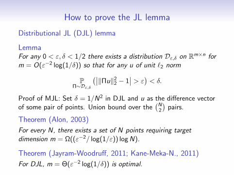
Distributional JL (DJL) lemma
LemmaFor any 0 < ε, δ < 1/2 there exists a distribution Dε,δ on Rm×n form = O(ε−2 log(1/δ)) so that for any u of unit `2 norm
PΠ∼Dε,δ
(∣∣‖Πu‖22 − 1
∣∣ > ε)< δ.
Proof of MJL: Set δ = 1/N2 in DJL and u as the difference vectorof some pair of points. Union bound over the
(N2
)pairs.
Theorem (Alon, 2003)
For every N, there exists a set of N points requiring targetdimension m = Ω((ε−2/ log(1/ε)) logN).
Theorem (Jayram-Woodruff, 2011; Kane-Meka-N., 2011)
For DJL, m = Θ(ε−2 log(1/δ)) is optimal.
How to prove the JL lemma
Distributional JL (DJL) lemma
LemmaFor any 0 < ε, δ < 1/2 there exists a distribution Dε,δ on Rm×n form = O(ε−2 log(1/δ)) so that for any u of unit `2 norm
PΠ∼Dε,δ
(∣∣‖Πu‖22 − 1
∣∣ > ε)< δ.
Proof of MJL: Set δ = 1/N2 in DJL and u as the difference vectorof some pair of points. Union bound over the
(N2
)pairs.
Theorem (Alon, 2003)
For every N, there exists a set of N points requiring targetdimension m = Ω((ε−2/ log(1/ε)) logN).
Theorem (Jayram-Woodruff, 2011; Kane-Meka-N., 2011)
For DJL, m = Θ(ε−2 log(1/δ)) is optimal.
Proving the distributional JL lemma
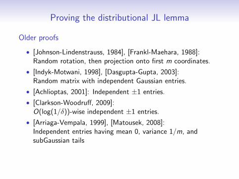
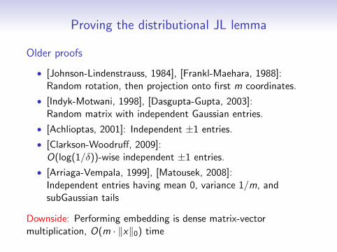
Older proofs
• [Johnson-Lindenstrauss, 1984], [Frankl-Maehara, 1988]:Random rotation, then projection onto first m coordinates.
• [Indyk-Motwani, 1998], [Dasgupta-Gupta, 2003]:Random matrix with independent Gaussian entries.
• [Achlioptas, 2001]: Independent ±1 entries.
• [Clarkson-Woodruff, 2009]:O(log(1/δ))-wise independent ±1 entries.
• [Arriaga-Vempala, 1999], [Matousek, 2008]:Independent entries having mean 0, variance 1/m, andsubGaussian tails
Downside: Performing embedding is dense matrix-vectormultiplication, O(m · ‖x‖0) time
Proving the distributional JL lemma
Older proofs
• [Johnson-Lindenstrauss, 1984], [Frankl-Maehara, 1988]:Random rotation, then projection onto first m coordinates.
• [Indyk-Motwani, 1998], [Dasgupta-Gupta, 2003]:Random matrix with independent Gaussian entries.
• [Achlioptas, 2001]: Independent ±1 entries.
• [Clarkson-Woodruff, 2009]:O(log(1/δ))-wise independent ±1 entries.
• [Arriaga-Vempala, 1999], [Matousek, 2008]:Independent entries having mean 0, variance 1/m, andsubGaussian tails
Downside: Performing embedding is dense matrix-vectormultiplication, O(m · ‖x‖0) time
Fast JL Transforms
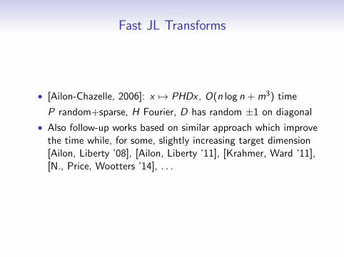
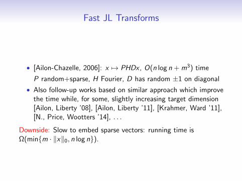
• [Ailon-Chazelle, 2006]: x 7→ PHDx , O(n log n + m3) time
P random+sparse, H Fourier, D has random ±1 on diagonal
• Also follow-up works based on similar approach which improvethe time while, for some, slightly increasing target dimension[Ailon, Liberty ’08], [Ailon, Liberty ’11], [Krahmer, Ward ’11],[N., Price, Wootters ’14], . . .
Downside: Slow to embed sparse vectors: running time isΩ(minm · ‖x‖0, n log n).
Fast JL Transforms
• [Ailon-Chazelle, 2006]: x 7→ PHDx , O(n log n + m3) time
P random+sparse, H Fourier, D has random ±1 on diagonal
• Also follow-up works based on similar approach which improvethe time while, for some, slightly increasing target dimension[Ailon, Liberty ’08], [Ailon, Liberty ’11], [Krahmer, Ward ’11],[N., Price, Wootters ’14], . . .
Downside: Slow to embed sparse vectors: running time isΩ(minm · ‖x‖0, n log n).

Where Do Sparse Vectors Show Up?
• Document as bag of words: ui = number of occurrences ofword i . Compare documents using cosine similarity.
n = lexicon size; most documents aren’t dictionaries
• Network traffic: ui ,j = #bytes sent from i to j
n = 264 (2256 in IPv6); most servers don’t talk to each other
• User ratings: ui ,j is user i ’s score for movie j on Netflix
n = #movies; most people haven’t rated all movies
• Streaming: u receives a stream of updates of the form: “addv to ui ”. Maintaining Πu requires calculating v · Πei .
• . . .
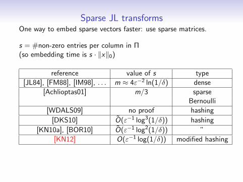
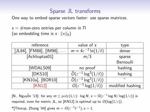
Sparse JL transformsOne way to embed sparse vectors faster: use sparse matrices.
s = #non-zero entries per column in Π(so embedding time is s · ‖x‖0)
reference value of s type
[JL84], [FM88], [IM98], . . . m ≈ 4ε−2 ln(1/δ) dense
[Achlioptas01] m/3 sparseBernoulli
[WDALS09] no proof hashing
[DKS10] O(ε−1 log3(1/δ)) hashing
[KN10a], [BOR10] O(ε−1 log2(1/δ)) ”
[KN12] O(ε−1 log(1/δ)) modified hashing
[N., Nguy˜en ’13]: for any m ≤ poly(1/ε) · logN, s = Ω(ε−1 logN/ log(1/ε)) is
required, even for metric JL, so [KN12] is optimal up to O(log(1/ε)).
*[Thorup, Zhang ’04] gives m = O(ε−2δ−1), s = 1.
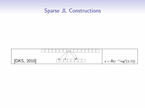
Sparse JL Constructions
[DKS, 2010] s = Θ(ε−1 log2(1/δ))
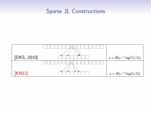
Sparse JL Constructions
[DKS, 2010] s = Θ(ε−1 log2(1/δ))
[KN12] s = Θ(ε−1 log(1/δ))
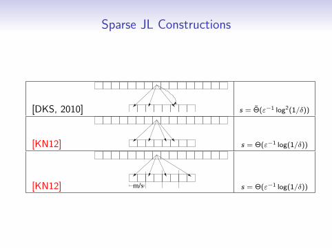
Sparse JL Constructions
[DKS, 2010] s = Θ(ε−1 log2(1/δ))
[KN12] s = Θ(ε−1 log(1/δ))
[KN12] m/s s = Θ(ε−1 log(1/δ))
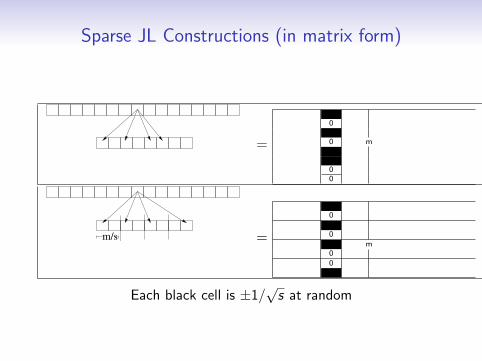
Sparse JL Constructions (in matrix form)
=
0
0 m
00
m/s =
0
0m
00
Each black cell is ±1/√s at random
Analysis
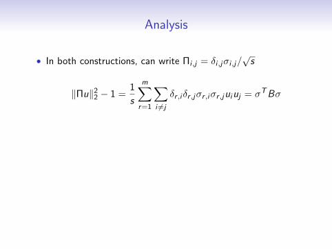
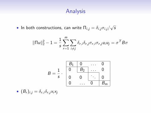
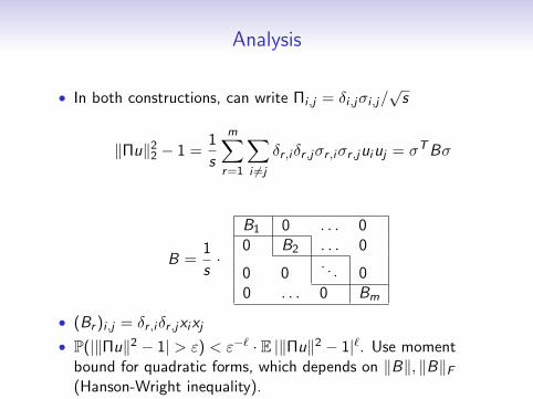
• In both constructions, can write Πi ,j = δi ,jσi ,j/√s
‖Πu‖22 − 1 =
1
s
m∑r=1
∑i 6=j
δr ,iδr ,jσr ,iσr ,juiuj = σTBσ
B =1
s·
B1 0 . . . 00 B2 . . . 0
0 0. . . 0
0 . . . 0 Bm
• (Br )i ,j = δr ,iδr ,jxixj
• P(|‖Πu‖2 − 1| > ε) < ε−` · E |‖Πu‖2 − 1|`. Use momentbound for quadratic forms, which depends on ‖B‖, ‖B‖F
(Hanson-Wright inequality).
Analysis
• In both constructions, can write Πi ,j = δi ,jσi ,j/√s
‖Πu‖22 − 1 =
1
s
m∑r=1
∑i 6=j
δr ,iδr ,jσr ,iσr ,juiuj = σTBσ
B =1
s·
B1 0 . . . 00 B2 . . . 0
0 0. . . 0
0 . . . 0 Bm
• (Br )i ,j = δr ,iδr ,jxixj
• P(|‖Πu‖2 − 1| > ε) < ε−` · E |‖Πu‖2 − 1|`. Use momentbound for quadratic forms, which depends on ‖B‖, ‖B‖F
(Hanson-Wright inequality).

What next?
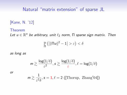
Natural “matrix extension” of sparse JL
[Kane, N. ’12]
TheoremLet u ∈ Rn be arbitrary, unit `2 norm, Π sparse sign matrix. Then
PΠ
(∣∣‖Πu‖2 − 1∣∣ > ε
)< δ
as long as
m &log(1/δ)
ε2, s &
log(1/δ)
ε, ` = log(1/δ)
or
m &1
ε2δ, s = 1, ` = 2 ([Thorup, Zhang′04])
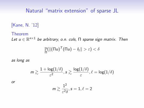
Natural “matrix extension” of sparse JL
[Kane, N. ’12]
TheoremLet u ∈ Rn×1 be arbitrary, o.n. cols, Π sparse sign matrix. Then
PΠ
(‖(Πu)T (Πu)− I1‖ > ε) < δ
as long as
m &1 + log(1/δ)
ε2, s &
log(1/δ)
ε, ` = log(1/δ)
or
m &12
ε2δ, s = 1, ` = 2
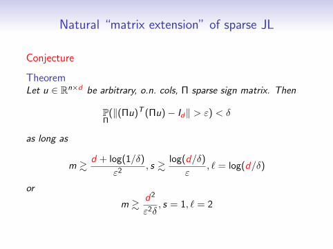
Natural “matrix extension” of sparse JL
Conjecture
TheoremLet u ∈ Rn×d be arbitrary, o.n. cols, Π sparse sign matrix. Then
PΠ
(‖(Πu)T (Πu)− Id‖ > ε) < δ
as long as
m &d + log(1/δ)
ε2, s &
log(d/δ)
ε, ` = log(d/δ)
or
m &d2
ε2δ, s = 1, ` = 2
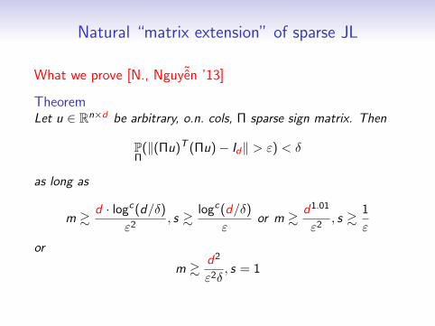
Natural “matrix extension” of sparse JL
What we prove [N., Nguy˜en ’13]
TheoremLet u ∈ Rn×d be arbitrary, o.n. cols, Π sparse sign matrix. Then
PΠ
(‖(Πu)T (Πu)− Id‖ > ε) < δ
as long as
m &d · logc (d/δ)
ε2, s &
logc (d/δ)
εor m &
d1.01
ε2, s &
1
ε
or
m &d2
ε2δ, s = 1
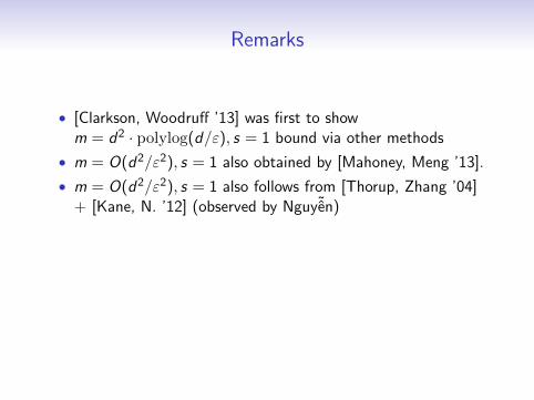
Remarks
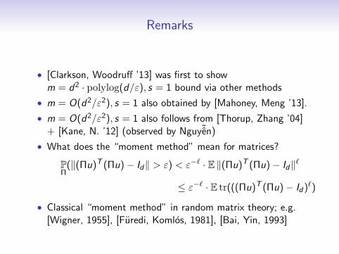
• [Clarkson, Woodruff ’13] was first to showm = d2 · polylog(d/ε), s = 1 bound via other methods
• m = O(d2/ε2), s = 1 also obtained by [Mahoney, Meng ’13].
• m = O(d2/ε2), s = 1 also follows from [Thorup, Zhang ’04]+ [Kane, N. ’12] (observed by Nguy˜en)
• What does the “moment method” mean for matrices?
PΠ
(‖(Πu)T (Πu)− Id‖ > ε) < ε−` · E ‖(Πu)T (Πu)− Id‖`
≤ ε−` · E tr(((Πu)T (Πu)− Id )`)
• Classical “moment method” in random matrix theory; e.g.[Wigner, 1955], [Furedi, Komlos, 1981], [Bai, Yin, 1993]
Remarks
• [Clarkson, Woodruff ’13] was first to showm = d2 · polylog(d/ε), s = 1 bound via other methods
• m = O(d2/ε2), s = 1 also obtained by [Mahoney, Meng ’13].
• m = O(d2/ε2), s = 1 also follows from [Thorup, Zhang ’04]+ [Kane, N. ’12] (observed by Nguy˜en)
• What does the “moment method” mean for matrices?
PΠ
(‖(Πu)T (Πu)− Id‖ > ε) < ε−` · E ‖(Πu)T (Πu)− Id‖`
≤ ε−` · E tr(((Πu)T (Πu)− Id )`)
• Classical “moment method” in random matrix theory; e.g.[Wigner, 1955], [Furedi, Komlos, 1981], [Bai, Yin, 1993]

Who cares about this matrix extension?

Motivation for matrix extension of sparse JL
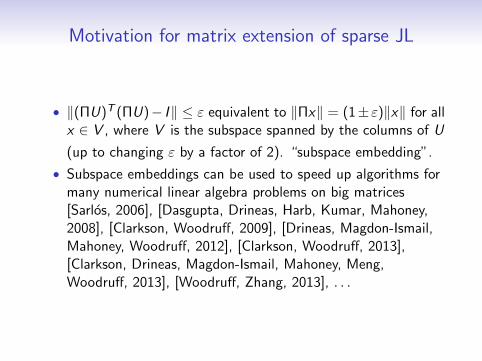
• ‖(ΠU)T (ΠU)− I‖ ≤ ε equivalent to ‖Πx‖ = (1± ε)‖x‖ for allx ∈ V , where V is the subspace spanned by the columns of U
(up to changing ε by a factor of 2). “subspace embedding”.
• Subspace embeddings can be used to speed up algorithms formany numerical linear algebra problems on big matrices[Sarlos, 2006], [Dasgupta, Drineas, Harb, Kumar, Mahoney,2008], [Clarkson, Woodruff, 2009], [Drineas, Magdon-Ismail,Mahoney, Woodruff, 2012], [Clarkson, Woodruff, 2013],[Clarkson, Drineas, Magdon-Ismail, Mahoney, Meng,Woodruff, 2013], [Woodruff, Zhang, 2013], . . .
• Sparse Π: can multiply ΠA in s · nnz(A) time for big matrix A.
Motivation for matrix extension of sparse JL
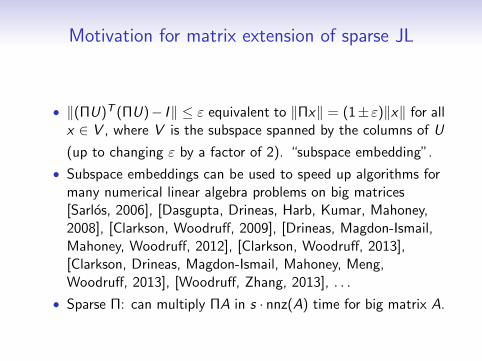
• ‖(ΠU)T (ΠU)− I‖ ≤ ε equivalent to ‖Πx‖ = (1± ε)‖x‖ for allx ∈ V , where V is the subspace spanned by the columns of U
(up to changing ε by a factor of 2). “subspace embedding”.
• Subspace embeddings can be used to speed up algorithms formany numerical linear algebra problems on big matrices[Sarlos, 2006], [Dasgupta, Drineas, Harb, Kumar, Mahoney,2008], [Clarkson, Woodruff, 2009], [Drineas, Magdon-Ismail,Mahoney, Woodruff, 2012], [Clarkson, Woodruff, 2013],[Clarkson, Drineas, Magdon-Ismail, Mahoney, Meng,Woodruff, 2013], [Woodruff, Zhang, 2013], . . .
• Sparse Π: can multiply ΠA in s · nnz(A) time for big matrix A.
Numerical linear algebra
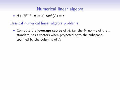
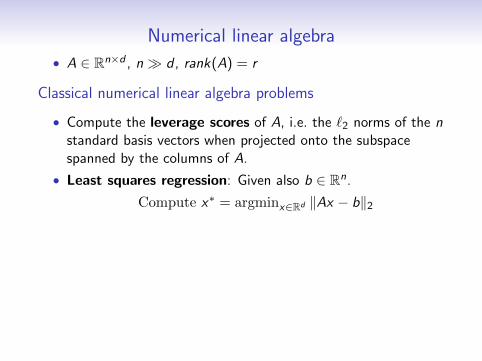
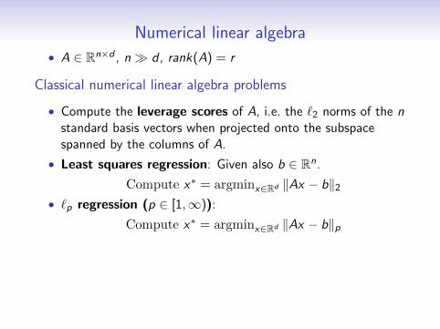
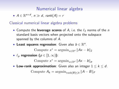
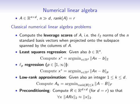
• A ∈ Rn×d , n d , rank(A) = r
Classical numerical linear algebra problems
• Compute the leverage scores of A, i.e. the `2 norms of the nstandard basis vectors when projected onto the subspacespanned by the columns of A.
• Least squares regression: Given also b ∈ Rn.
Compute x∗ = argminx∈Rd ‖Ax − b‖2
• `p regression (p ∈ [1,∞)):
Compute x∗ = argminx∈Rd ‖Ax − b‖p
• Low-rank approximation: Given also an integer 1 ≤ k ≤ d .
Compute Ak = argminrank(B)≤k ‖A− B‖F
• Preconditioning: Compute R ∈ Rd×d (for d = r) so that
∀x ‖ARx‖2 ≈ ‖x‖2
Numerical linear algebra
• A ∈ Rn×d , n d , rank(A) = r
Classical numerical linear algebra problems
• Compute the leverage scores of A, i.e. the `2 norms of the nstandard basis vectors when projected onto the subspacespanned by the columns of A.
• Least squares regression: Given also b ∈ Rn.
Compute x∗ = argminx∈Rd ‖Ax − b‖2
• `p regression (p ∈ [1,∞)):
Compute x∗ = argminx∈Rd ‖Ax − b‖p
• Low-rank approximation: Given also an integer 1 ≤ k ≤ d .
Compute Ak = argminrank(B)≤k ‖A− B‖F
• Preconditioning: Compute R ∈ Rd×d (for d = r) so that
∀x ‖ARx‖2 ≈ ‖x‖2
Computationally efficient solutions
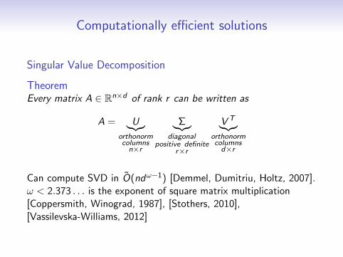
Singular Value Decomposition
TheoremEvery matrix A ∈ Rn×d of rank r can be written as
A = U︸︷︷︸orthonormcolumns
n×r
Σ︸︷︷︸diagonal
positive definiter×r
V T︸︷︷︸orthonormcolumns
d×r
Can compute SVD in O(ndω−1) [Demmel, Dumitriu, Holtz, 2007].ω < 2.373 . . . is the exponent of square matrix multiplication[Coppersmith, Winograd, 1987], [Stothers, 2010],[Vassilevska-Williams, 2012]
Computationally efficient solutions
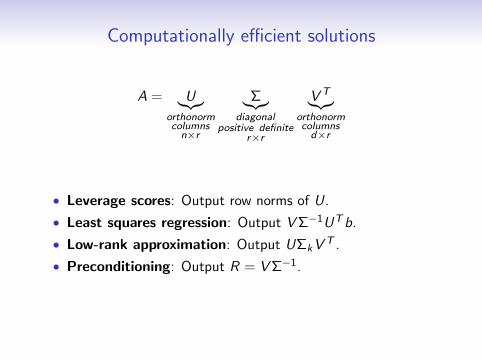
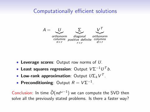
A = U︸︷︷︸orthonormcolumns
n×r
Σ︸︷︷︸diagonal
positive definiter×r
V T︸︷︷︸orthonormcolumns
d×r
• Leverage scores: Output row norms of U.
• Least squares regression: Output VΣ−1UTb.
• Low-rank approximation: Output UΣkVT .
• Preconditioning: Output R = VΣ−1.
Conclusion: In time O(ndω−1) we can compute the SVD thensolve all the previously stated problems. Is there a faster way?
Computationally efficient solutions
A = U︸︷︷︸orthonormcolumns
n×r
Σ︸︷︷︸diagonal
positive definiter×r
V T︸︷︷︸orthonormcolumns
d×r
• Leverage scores: Output row norms of U.
• Least squares regression: Output VΣ−1UTb.
• Low-rank approximation: Output UΣkVT .
• Preconditioning: Output R = VΣ−1.
Conclusion: In time O(ndω−1) we can compute the SVD thensolve all the previously stated problems. Is there a faster way?
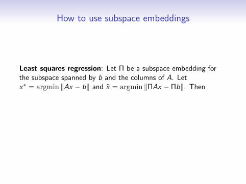
How to use subspace embeddings
Least squares regression: Let Π be a subspace embedding forthe subspace spanned by b and the columns of A. Letx∗ = argmin ‖Ax − b‖ and x = argmin ‖ΠAx − Πb‖. Then
(1− ε)‖Ax − b‖ ≤‖ΠAx−Πb‖ ≤ ‖ΠAx∗−Πb‖≤ (1 + ε)‖Ax∗ − b‖
⇒ ‖Ax − b‖ ≤(
1 + ε
1− ε
)· ‖Ax∗ − b‖

How to use subspace embeddings
Least squares regression: Let Π be a subspace embedding forthe subspace spanned by b and the columns of A. Letx∗ = argmin ‖Ax − b‖ and x = argmin ‖ΠAx − Πb‖. Then
(1− ε)‖Ax − b‖ ≤‖ΠAx−Πb‖ ≤ ‖ΠAx∗−Πb‖≤ (1 + ε)‖Ax∗ − b‖
⇒ ‖Ax − b‖ ≤(
1 + ε
1− ε
)· ‖Ax∗ − b‖
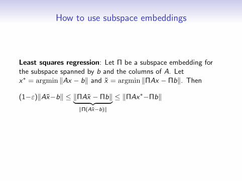
How to use subspace embeddings
Least squares regression: Let Π be a subspace embedding forthe subspace spanned by b and the columns of A. Letx∗ = argmin ‖Ax − b‖ and x = argmin ‖ΠAx − Πb‖. Then
(1−ε)‖Ax−b‖ ≤ ‖ΠAx − Πb‖︸ ︷︷ ︸‖Π(Ax−b)‖
≤ ‖ΠAx∗−Πb‖≤ (1 + ε)‖Ax∗ − b‖
⇒ ‖Ax − b‖ ≤(
1 + ε
1− ε
)· ‖Ax∗ − b‖
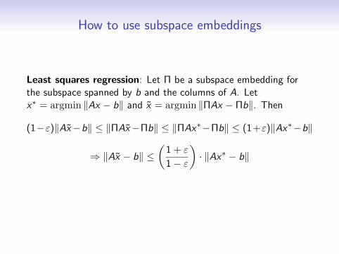
How to use subspace embeddings
Least squares regression: Let Π be a subspace embedding forthe subspace spanned by b and the columns of A. Letx∗ = argmin ‖Ax − b‖ and x = argmin ‖ΠAx − Πb‖. Then
(1−ε)‖Ax−b‖ ≤ ‖ΠAx−Πb‖ ≤ ‖ΠAx∗−Πb‖ ≤ (1+ε)‖Ax∗−b‖
⇒ ‖Ax − b‖ ≤(
1 + ε
1− ε
)· ‖Ax∗ − b‖
Computing SVD of ΠA takes time O(mdω−1), which is muchfaster than O(ndω−1) since m n.
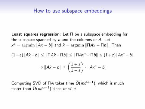
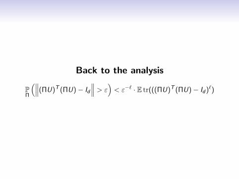
Back to the analysis
PΠ
(∥∥∥(ΠU)T (ΠU)− Id
∥∥∥ > ε)< ε−` · E tr(((ΠU)T (ΠU)− Id )`)
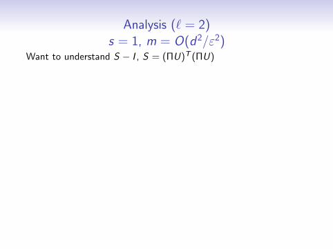
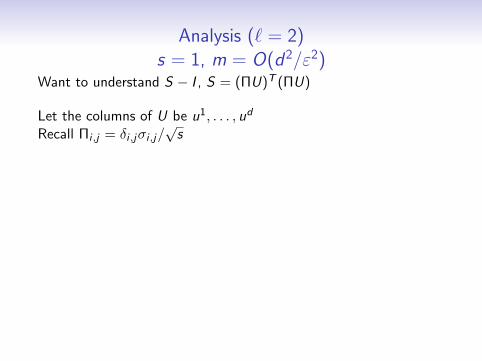
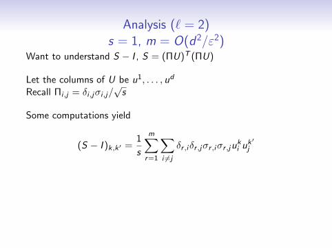
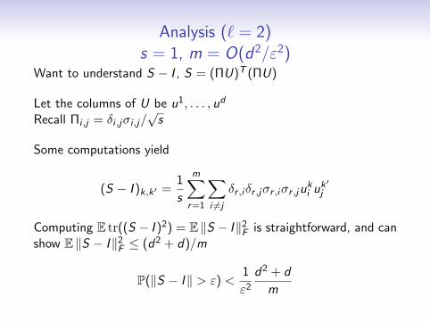
Analysis (` = 2)s = 1, m = O(d2/ε2)
Want to understand S − I , S = (ΠU)T (ΠU)
Let the columns of U be u1, . . . , ud
Recall Πi ,j = δi ,jσi ,j/√s
Some computations yield
(S − I )k,k ′ =1
s
m∑r=1
∑i 6=j
δr ,iδr ,jσr ,iσr ,juki u
k ′j
Computing E tr((S − I )2) = E ‖S − I‖2F is straightforward, and can
show E ‖S − I‖2F ≤ (d2 + d)/m
P(‖S − I‖ > ε) <1
ε2
d2 + d
m
Set m ≥ δ−1(d2 + d)/ε2 for success probability 1− δ
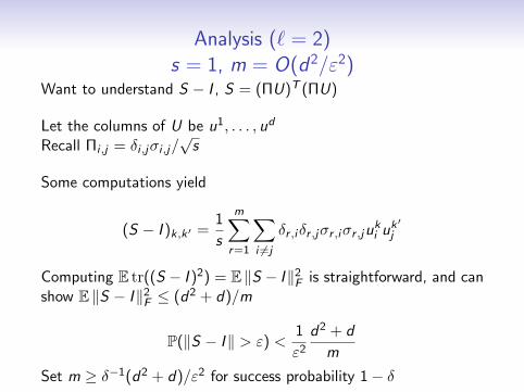
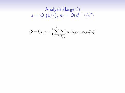
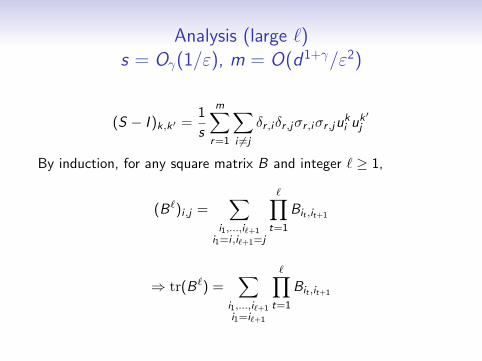
Analysis (large `)s = Oγ(1/ε), m = O(d1+γ/ε2)
(S − I )k,k ′ =1
s
m∑r=1
∑i 6=j
δr ,iδr ,jσr ,iσr ,juki u
k ′j
By induction, for any square matrix B and integer ` ≥ 1,
(B`)i ,j =∑
i1,...,i`+1i1=i ,i`+1=j
∏t=1
Bit ,it+1
⇒ tr(B`) =∑
i1,...,i`+1i1=i`+1
∏t=1
Bit ,it+1
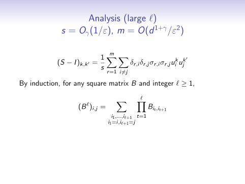
Analysis (large `)s = Oγ(1/ε), m = O(d1+γ/ε2)
(S − I )k,k ′ =1
s
m∑r=1
∑i 6=j
δr ,iδr ,jσr ,iσr ,juki u
k ′j
By induction, for any square matrix B and integer ` ≥ 1,
(B`)i ,j =∑
i1,...,i`+1i1=i ,i`+1=j
∏t=1
Bit ,it+1
⇒ tr(B`) =∑
i1,...,i`+1i1=i`+1
∏t=1
Bit ,it+1
Analysis (large `)s = Oγ(1/ε), m = O(d1+γ/ε2)
(S − I )k,k ′ =1
s
m∑r=1
∑i 6=j
δr ,iδr ,jσr ,iσr ,juki u
k ′j
By induction, for any square matrix B and integer ` ≥ 1,
(B`)i ,j =∑
i1,...,i`+1i1=i ,i`+1=j
∏t=1
Bit ,it+1
⇒ tr(B`) =∑
i1,...,i`+1i1=i`+1
∏t=1
Bit ,it+1
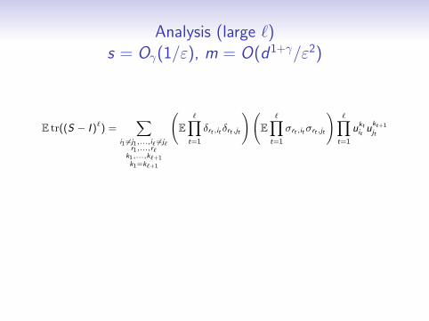
Analysis (large `)s = Oγ(1/ε), m = O(d1+γ/ε2)
E tr((S − I )`) =∑
i1 6=j1,...,i` 6=j`r1,...,r`
k1,...,k`+1k1=k`+1
(E∏t=1
δrt ,it δrt ,jt
)(E∏t=1
σrt ,itσrt ,jt
)∏t=1
uktitu
kt+1jt
The strategy: Associate each monomial in summation above witha graph, group monomials that have the same graph, and estimatethe contribution of each graph then do some combinatorics
(a common strategy; see [Wigner, 1955], [Furedi, Komlos, 1981],[Bai, Yin, 1993])
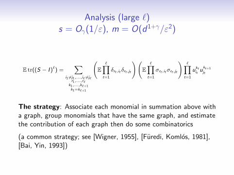
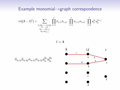
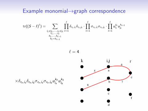
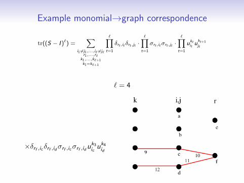
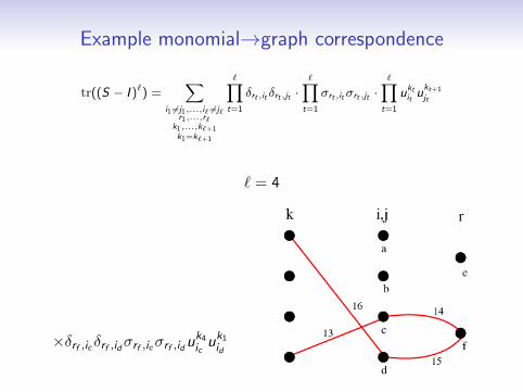
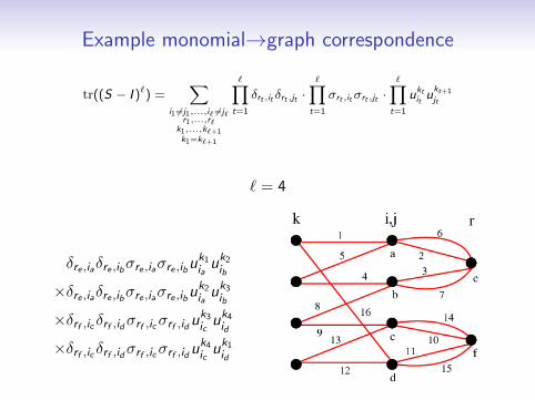
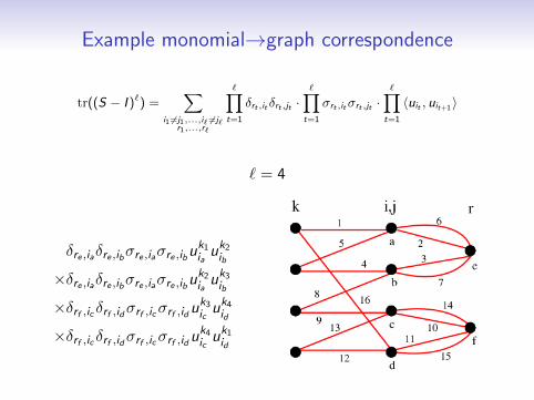
Example monomial→graph correspondence
tr((S − I )`) =∑
i1 6=j1,...,i` 6=j`r1,...,r`
k1,...,k`+1k1=k`+1
∏t=1
δrt ,it δrt ,jt ·∏t=1
σrt ,itσrt ,jt ·∏t=1
uktitu
kt+1jt
` = 4
δre ,iaδre ,ibσre ,iaσre ,ibuk1iauk2
ib
×δre ,iaδre ,ibσre ,iaσre ,ibuk2iauk3
ib
×δrf ,ic δrf ,idσrf ,icσrf ,iduk3icuk4
id
×δrf ,ic δrf ,idσrf ,icσrf ,iduk4icuk1
id
Example monomial→graph correspondence
tr((S − I )`) =∑
i1 6=j1,...,i` 6=j`r1,...,r`
∏t=1
δrt ,it δrt ,jt ·∏t=1
σrt ,itσrt ,jt ·∏t=1
〈uit , uit+1〉
` = 4
δre ,iaδre ,ibσre ,iaσre ,ibuk1iauk2
ib
×δre ,iaδre ,ibσre ,iaσre ,ibuk2iauk3
ib
×δrf ,ic δrf ,idσrf ,icσrf ,iduk3icuk4
id
×δrf ,ic δrf ,idσrf ,icσrf ,iduk4icuk1
id
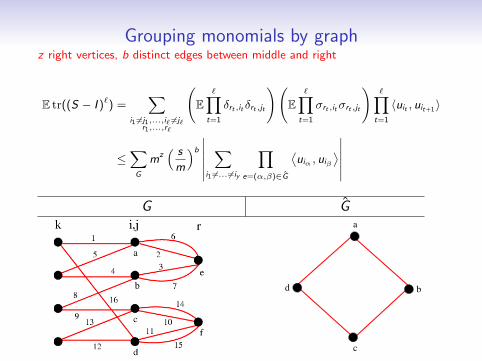
Grouping monomials by graphz right vertices, b distinct edges between middle and right
E tr((S − I )`) =∑
i1 6=j1,...,i` 6=j`r1,...,r`
(E∏t=1
δrt ,it δrt ,jt
)(E∏t=1
σrt ,itσrt ,jt
)∏t=1
〈uit , uit+1〉
≤∑
G
mz( s
m
)b
∣∣∣∣∣∣∑
i1 6=... 6=iy
∏e=(α,β)∈G
⟨uiα , uiβ
⟩∣∣∣∣∣∣G G
a
b
c
d
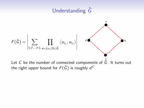
Understanding G
F (G ) =
∣∣∣∣∣∣∑
i1 6=... 6=iy
∏e=(α,β)∈G
⟨uiα , uiβ
⟩∣∣∣∣∣∣
a
b
c
d
Let C be the number of connected components of G . It turns outthe right upper bound for F (G ) is roughly dC
• Can get dC bound if all edges in G have even multiplicity
• How about G where this isn’t the case, e.g. as above?
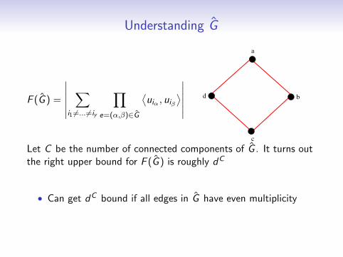
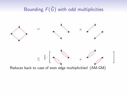
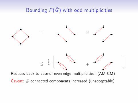
Bounding F (G ) with odd multiplicities
a
b
c
d
=
≤12 ·
[
d
a
b
c
a
b
c
d
×
+
a
b
c
d
a
b
c
d
]Reduces back to case of even edge multiplicities! (AM-GM)
Caveat: # connected components increased (unacceptable)
Bounding F (G ) with odd multiplicities
a
b
c
d
=
≤12 ·
[
d
a
b
c
a
b
c
d
×
+
a
b
c
d
a
b
c
d
]Reduces back to case of even edge multiplicities! (AM-GM)
Caveat: # connected components increased (unacceptable)
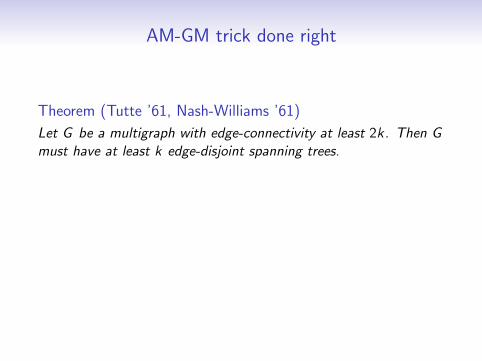
AM-GM trick done right
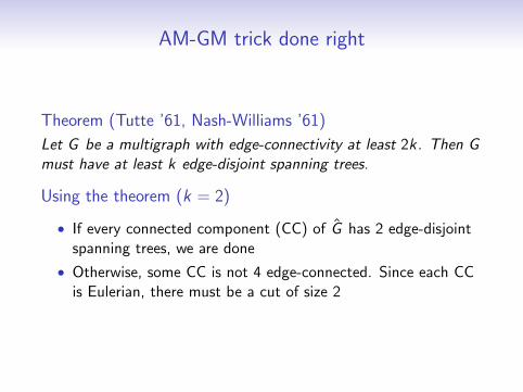
Theorem (Tutte ’61, Nash-Williams ’61)
Let G be a multigraph with edge-connectivity at least 2k. Then Gmust have at least k edge-disjoint spanning trees.
Using the theorem (k = 2)
• If every connected component (CC) of G has 2 edge-disjointspanning trees, we are done
• Otherwise, some CC is not 4 edge-connected. Since each CCis Eulerian, there must be a cut of size 2
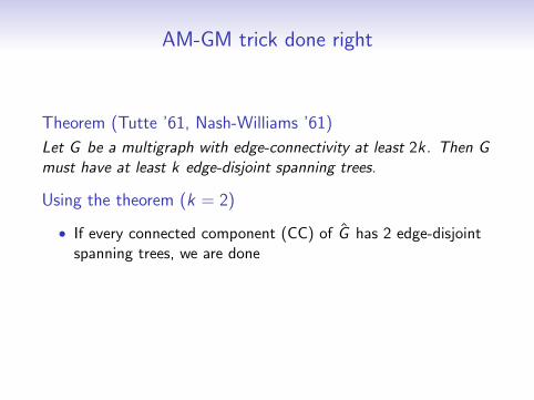
AM-GM trick done right
Theorem (Tutte ’61, Nash-Williams ’61)
Let G be a multigraph with edge-connectivity at least 2k. Then Gmust have at least k edge-disjoint spanning trees.
Using the theorem (k = 2)
• If every connected component (CC) of G has 2 edge-disjointspanning trees, we are done
• Otherwise, some CC is not 4 edge-connected. Since each CCis Eulerian, there must be a cut of size 2
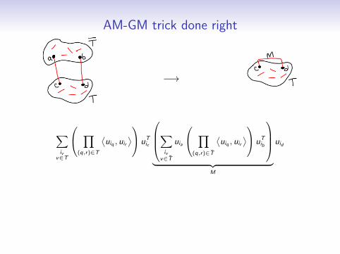
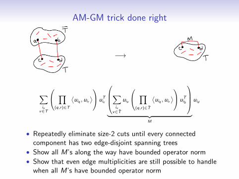
AM-GM trick done right
−→
∑iv
v∈T
∏(q,r)∈T
⟨uiq , uir
⟩ uTic
∑iv
v∈T
uia
∏(q,r)∈T
⟨uiq , uir
⟩ uTib
︸ ︷︷ ︸
M
uid
• Repeatedly eliminate size-2 cuts until every connectedcomponent has two edge-disjoint spanning trees
• Show all M’s along the way have bounded operator norm
• Show that even edge multiplicities are still possible to handlewhen all M’s have bounded operator norm

Conclusion

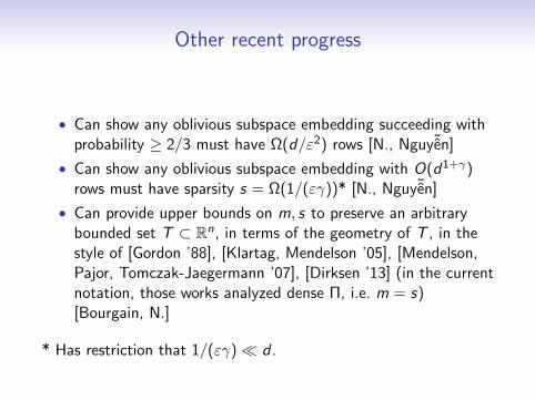
Other recent progress
• Can show any oblivious subspace embedding succeeding withprobability ≥ 2/3 must have Ω(d/ε2) rows [N., Nguy˜en]
• Can show any oblivious subspace embedding with O(d1+γ)rows must have sparsity s = Ω(1/(εγ))* [N., Nguy˜en]
• Can provide upper bounds on m, s to preserve an arbitrarybounded set T ⊂ Rn, in terms of the geometry of T , in thestyle of [Gordon ’88], [Klartag, Mendelson ’05], [Mendelson,Pajor, Tomczak-Jaegermann ’07], [Dirksen ’13] (in the currentnotation, those works analyzed dense Π, i.e. m = s)[Bourgain, N.]
* Has restriction that 1/(εγ) d .
Open Problems
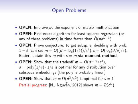
• OPEN: Improve ω, the exponent of matrix multiplication
• OPEN: Find exact algorithm for least squares regression (orany of these problems) in time faster than O(ndω−1)
• OPEN: Prove conjecture: to get subsp. embedding with prob.1− δ, can set m = O((d + log(1/δ))/ε2), s = O(log(d/δ)/ε).Easier: obtain this m with s = m via moment method.
• OPEN: Show that the tradeoff m = O(d1+γ/ε2),s = poly(1/γ) · 1/ε is optimal for any distribution oversubspace embeddings (the poly is probably linear)
• OPEN: Show that m = Ω(d2/ε2) is optimal for s = 1
Partial progress: [N., Nguy˜en, 2012] shows m = Ω(d2)