DFT AND IDFT - kth.se · PDF fileFAST FOURIER TRANSFORM (FFT) FFT is a fast algorithm for...
4
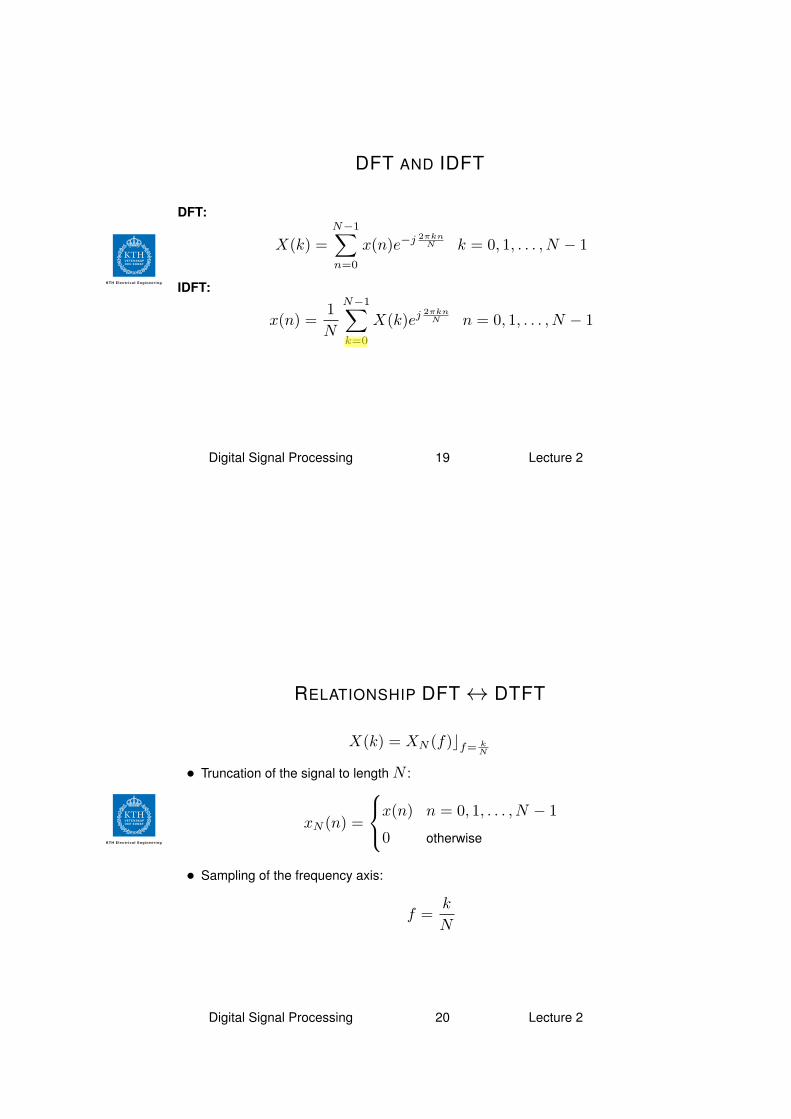
DFT AND IDFT DFT: X (k)= N-1 n=0 x(n)e -j 2πkn N k =0, 1,...,N − 1 IDFT: x(n)= 1 N N-1 k=0 X (k)e j 2πkn N n =0, 1,...,N − 1 Digital Signal Processing 19 Lecture 2 RELATIONSHIP DFT ↔ DTFT X (k)= X N (f )⌋ f = k N • Truncation of the signal to length N : x N (n)= x(n) n =0, 1,...,N − 1 0 otherwise • Sampling of the frequency axis: f = k N Digital Signal Processing 20 Lecture 2
Transcript of DFT AND IDFT - kth.se · PDF fileFAST FOURIER TRANSFORM (FFT) FFT is a fast algorithm for...
DFT AND IDFT
DFT:
X(k) =
N−1∑
n=0
x(n)e−j 2πknN k = 0, 1, . . . , N − 1
IDFT:
x(n) =1
N
N−1∑
k=0
X(k)ej2πkn
N n = 0, 1, . . . , N − 1
Digital Signal Processing 19 Lecture 2
RELATIONSHIP DFT ↔ DTFT
X(k) = XN (f)⌋f= kN
• Truncation of the signal to length N :
xN (n) =
x(n) n = 0, 1, . . . , N − 1
0 otherwise
• Sampling of the frequency axis:
f =k
N
Digital Signal Processing 20 Lecture 2
matben
Highlight
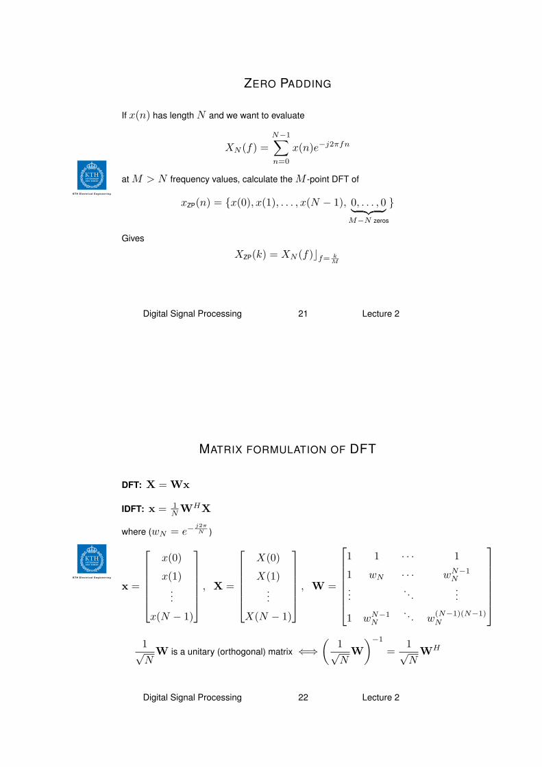
ZERO PADDING
If x(n) has length N and we want to evaluate
XN (f) =
N−1∑
n=0
x(n)e−j2πfn
at M > N frequency values, calculate the M -point DFT of
xZP(n) = {x(0), x(1), . . . , x(N − 1), 0, . . . , 0︸ ︷︷ ︸
M−N zeros
}
Gives
XZP(k) = XN (f)⌋f= kM
Digital Signal Processing 21 Lecture 2
MATRIX FORMULATION OF DFT
DFT: X = Wx
IDFT: x = 1NW
HX
where (wN = e−j2π
N )
x =
x(0)
x(1)...
x(N − 1)
, X =
X(0)
X(1)...
X(N − 1)
, W =
1 1 · · · 1
1 wN · · · wN−1N
.
.
.. . .
.
.
.
1 wN−1N
. . . w(N−1)(N−1)N
1√N
W is a unitary (orthogonal) matrix ⇐⇒(
1√N
W
)−1
=1√N
WH
Digital Signal Processing 22 Lecture 2
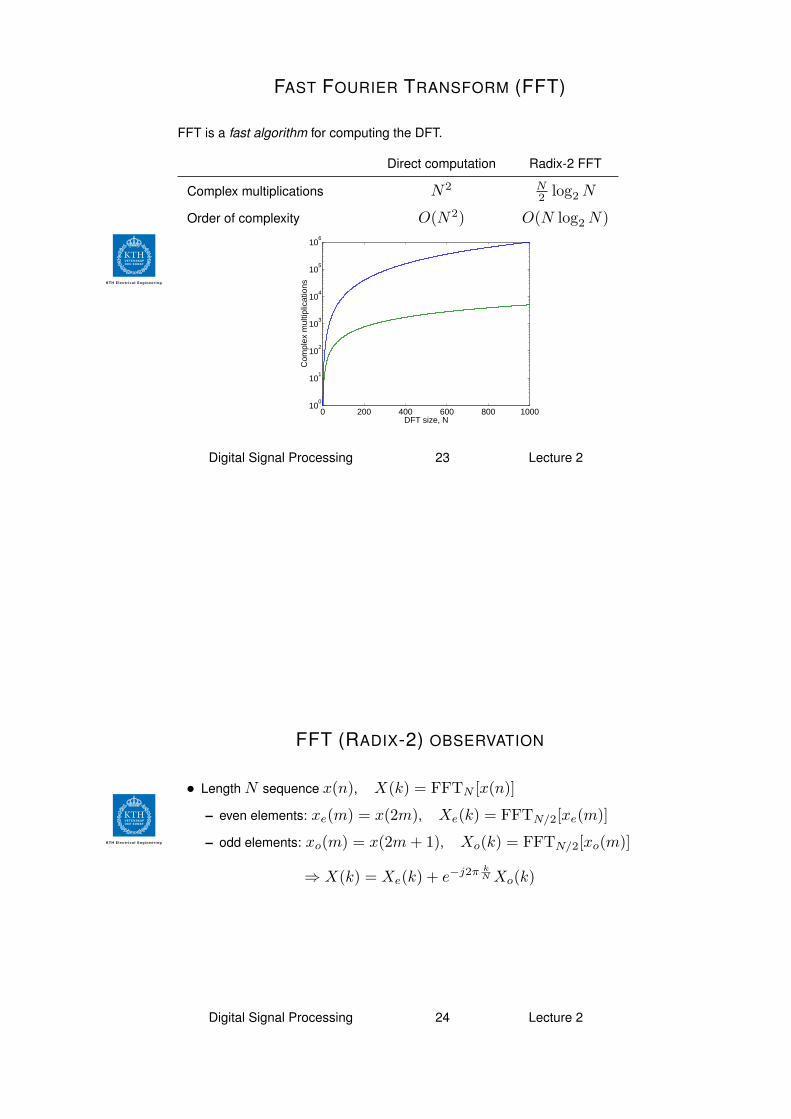
FAST FOURIER TRANSFORM (FFT)
FFT is a fast algorithm for computing the DFT.
Direct computation Radix-2 FFT
Complex multiplications N2 N2 log2 N
Order of complexity O(N2) O(N log2 N)
0 200 400 600 800 100010
0
101
102
103
104
105
106
DFT size, N
Com
plex
mul
tiplic
atio
ns
Digital Signal Processing 23 Lecture 2
FFT (RADIX-2) OBSERVATION
• Length N sequence x(n), X(k) = FFTN [x(n)]
– even elements: xe(m) = x(2m), Xe(k) = FFTN/2[xe(m)]
– odd elements: xo(m) = x(2m+ 1), Xo(k) = FFTN/2[xo(m)]
⇒ X(k) = Xe(k) + e−j2π kN Xo(k)
Digital Signal Processing 24 Lecture 2
REMARKS, FFT
• Several different kinds of FFTs! These provide trade-offs between
multiplications, additions and memory usage.
• Other important aspects are parallel computation, quantization effects and bit
representation in each stage.
• Renewed interest in FFT algorithms due to OFDM (Orthogonal Frequency
Division Multiplexing) used in ADSL, Wireless LAN, 4G wireless (LTE) and
digital radio broadcast (DAB).
Digital Signal Processing 25 Lecture 2


![DFT – Nuts & Bolts, Approximations [based on Chapter 3, Sholl & Steckel]](https://static.fdocument.org/doc/165x107/56814c92550346895db9a5ce/dft-nuts-bolts-approximations-based-on-chapter-3-sholl-steckel.jpg)