1

DESIGN OPTIMIZATION STUDY ON AN ULTRAFAST SMART (SMA RESETTABLE) LATCH

by

Shishira Nagesh Won Hee Kim

ME 555-09-02

Winter 2009 Final Report

ABSTRACT An active T-latch with automatic release and reset capabilities was designed and

fabricated by Redmond et al. [1]. The latch demonstrated the technology for an automotive panel

lockdown. The T-latch can be broadly divided into two parts based on the functionality of each.

The first part consists of the shaft, shoulder, base and the ramps to be referred henceforth as the

T-latch. The spool-packaged Shape Memory Alloy (SMA) actuator is the second component of

the latch. The purpose of this optimization study is to make this device more suitable for use in

the automotive sector where two of the main concerns are net volume (analogous to the weight)

and power consumption of the device. An attempt will be made to optimize the T-latch for yet

another important industry consideration, minimal footprint analogous to the packaging volume.

Design tradeoffs and results are discussed for the individual subsystems and for the overall

system.

2

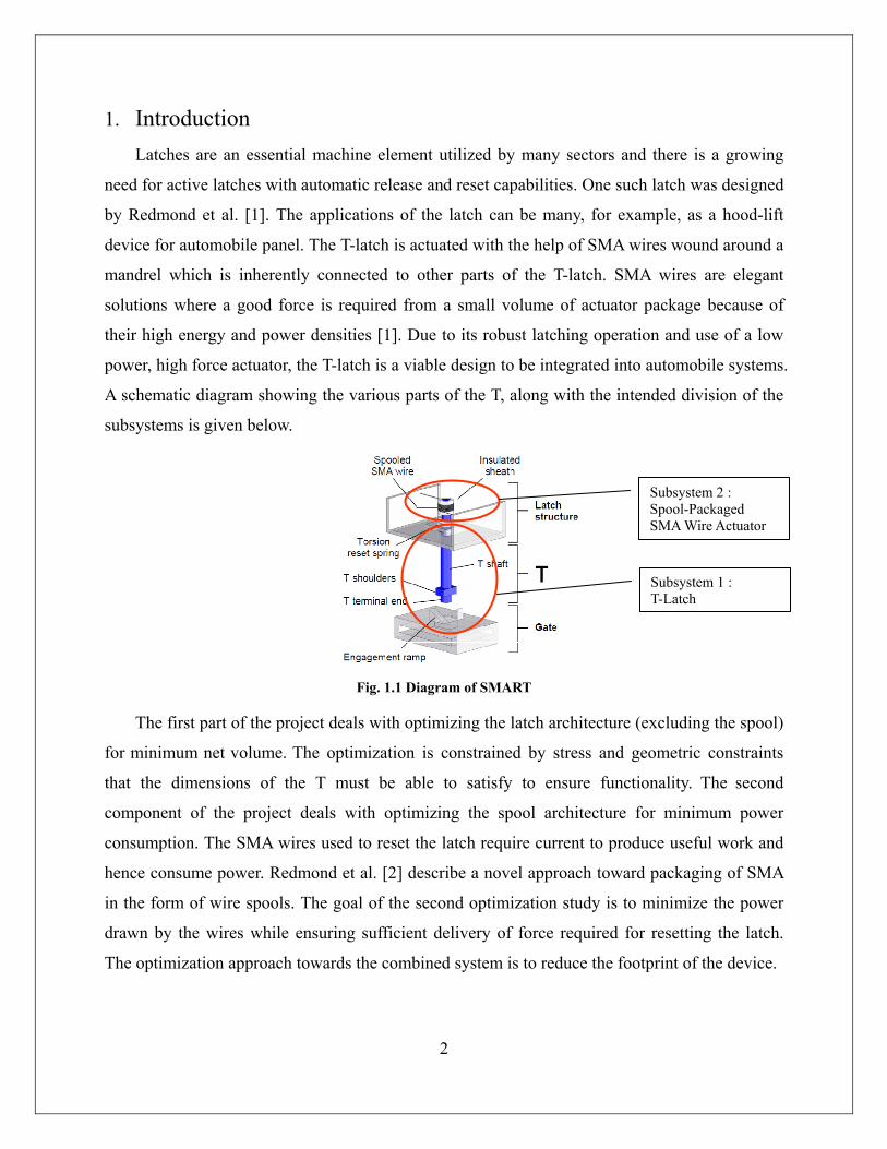
1. Introduction Latches are an essential machine element utilized by many sectors and there is a growing

need for active latches with automatic release and reset capabilities. One such latch was designed

by Redmond et al. [1]. The applications of the latch can be many, for example, as a hood-lift

device for automobile panel. The T-latch is actuated with the help of SMA wires wound around a

mandrel which is inherently connected to other parts of the T-latch. SMA wires are elegant

solutions where a good force is required from a small volume of actuator package because of

their high energy and power densities [1]. Due to its robust latching operation and use of a low

power, high force actuator, the T-latch is a viable design to be integrated into automobile systems.

A schematic diagram showing the various parts of the T, along with the intended division of the

subsystems is given below.

Fig. 1.1 Diagram of SMART

The first part of the project deals with optimizing the latch architecture (excluding the spool)

for minimum net volume. The optimization is constrained by stress and geometric constraints

that the dimensions of the T must be able to satisfy to ensure functionality. The second

component of the project deals with optimizing the spool architecture for minimum power

consumption. The SMA wires used to reset the latch require current to produce useful work and

hence consume power. Redmond et al. [2] describe a novel approach toward packaging of SMA

in the form of wire spools. The goal of the second optimization study is to minimize the power

drawn by the wires while ensuring sufficient delivery of force required for resetting the latch.

The optimization approach towards the combined system is to reduce the footprint of the device.

Subsystem 2 : Spool-Packaged SMA Wire Actuator

Subsystem 1 : T-Latch

3

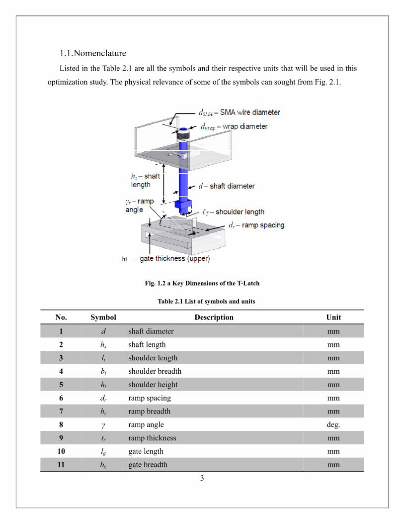
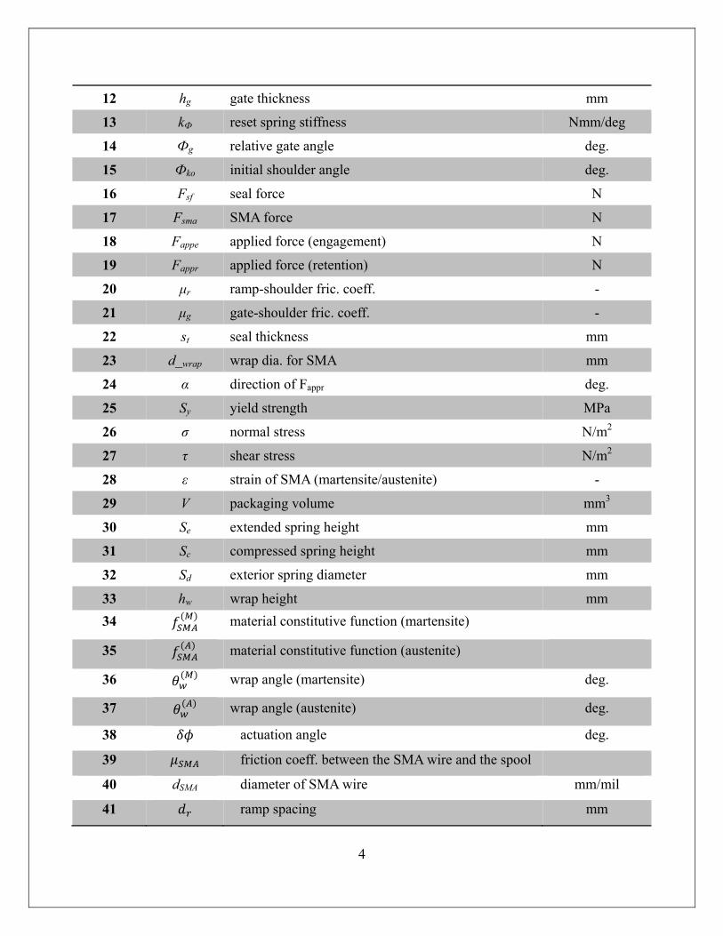
1.1. Nomenclature Listed in the Table 2.1 are all the symbols and their respective units that will be used in this

optimization study. The physical relevance of some of the symbols can sought from Fig. 2.1.

Fig. 1.2 a Key Dimensions of the T-Latch

No. Symbol Description Unit

1 d shaft diameter mm

2 hs shaft length mm

3 lt shoulder length mm

4 bt shoulder breadth mm

5 ht shoulder height mm

6 dr ramp spacing mm

7 br ramp breadth mm

8 γ ramp angle deg.

9 tr ramp thickness mm

10 lg gate length mm

11 bg gate breadth mm

ht

Table 2.1 List of symbols and units

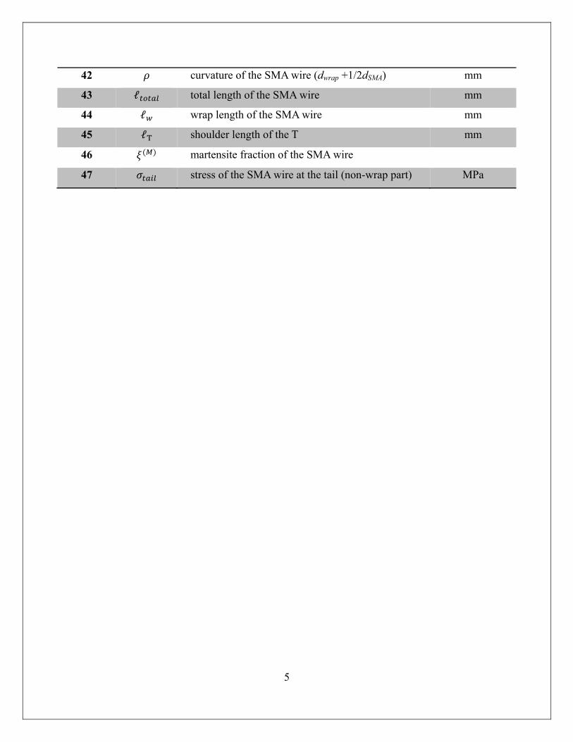
4

12 hg gate thickness mm

13 kФ reset spring stiffness Nmm/deg

14 Фg relative gate angle deg.

15 Фko initial shoulder angle deg.

16 Fsf seal force N

17 Fsma SMA force N

18 Fappe applied force (engagement) N

19 Fappr applied force (retention) N

20 μr ramp-shoulder fric. coeff. -

21 μg gate-shoulder fric. coeff. -

22 st seal thickness mm

23 d_wrap wrap dia. for SMA mm

24 α direction of Fappr deg.

25 Sy yield strength MPa

26 σ normal stress N/m2

27 τ shear stress N/m2

28 ε strain of SMA (martensite/austenite) -

29 V packaging volume mm3

30 Se extended spring height mm

31 Sc compressed spring height mm

32 Sd exterior spring diameter mm

33 hw wrap height mm 34 material constitutive function (martensite)

35 material constitutive function (austenite)

36 wrap angle (martensite) deg.

37 wrap angle (austenite) deg.

38 actuation angle deg.

39 friction coeff. between the SMA wire and the spool

40 dSMA diameter of SMA wire mm/mil

41 ramp spacing mm

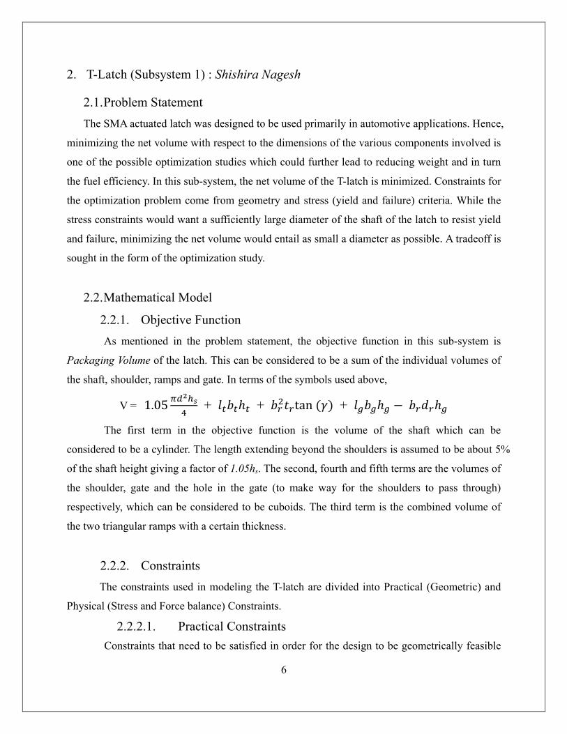
5

42 curvature of the SMA wire (dwrap +1/2dSMA) mm

43 ℓ total length of the SMA wire mm

44 ℓ wrap length of the SMA wire mm

45 ℓT shoulder length of the T mm

46 martensite fraction of the SMA wire

47 stress of the SMA wire at the tail (non-wrap part) MPa

6

2. T-Latch (Subsystem 1) : Shishira Nagesh

2.1. Problem Statement The SMA actuated latch was designed to be used primarily in automotive applications. Hence,

minimizing the net volume with respect to the dimensions of the various components involved is

one of the possible optimization studies which could further lead to reducing weight and in turn

the fuel efficiency. In this sub-system, the net volume of the T-latch is minimized. Constraints for

the optimization problem come from geometry and stress (yield and failure) criteria. While the

stress constraints would want a sufficiently large diameter of the shaft of the latch to resist yield

and failure, minimizing the net volume would entail as small a diameter as possible. A tradeoff is

sought in the form of the optimization study.

2.2. Mathematical Model

2.2.1. Objective Function As mentioned in the problem statement, the objective function in this sub-system is

Packaging Volume of the latch. This can be considered to be a sum of the individual volumes of

the shaft, shoulder, ramps and gate. In terms of the symbols used above,

V = 1.05 + + tan +

The first term in the objective function is the volume of the shaft which can be

considered to be a cylinder. The length extending beyond the shoulders is assumed to be about 5%

of the shaft height giving a factor of 1.05hs. The second, fourth and fifth terms are the volumes of

the shoulder, gate and the hole in the gate (to make way for the shoulders to pass through)

respectively, which can be considered to be cuboids. The third term is the combined volume of

the two triangular ramps with a certain thickness.

2.2.2. Constraints The constraints used in modeling the T-latch are divided into Practical (Geometric) and

Physical (Stress and Force balance) Constraints.

2.2.2.1. Practical Constraints Constraints that need to be satisfied in order for the design to be geometrically feasible

7

are listed below.

i) The shoulder length must be at least greater than or equal to the ramp spacing so that the

shoulder does not just pass into the gap without making contact with the ramps.

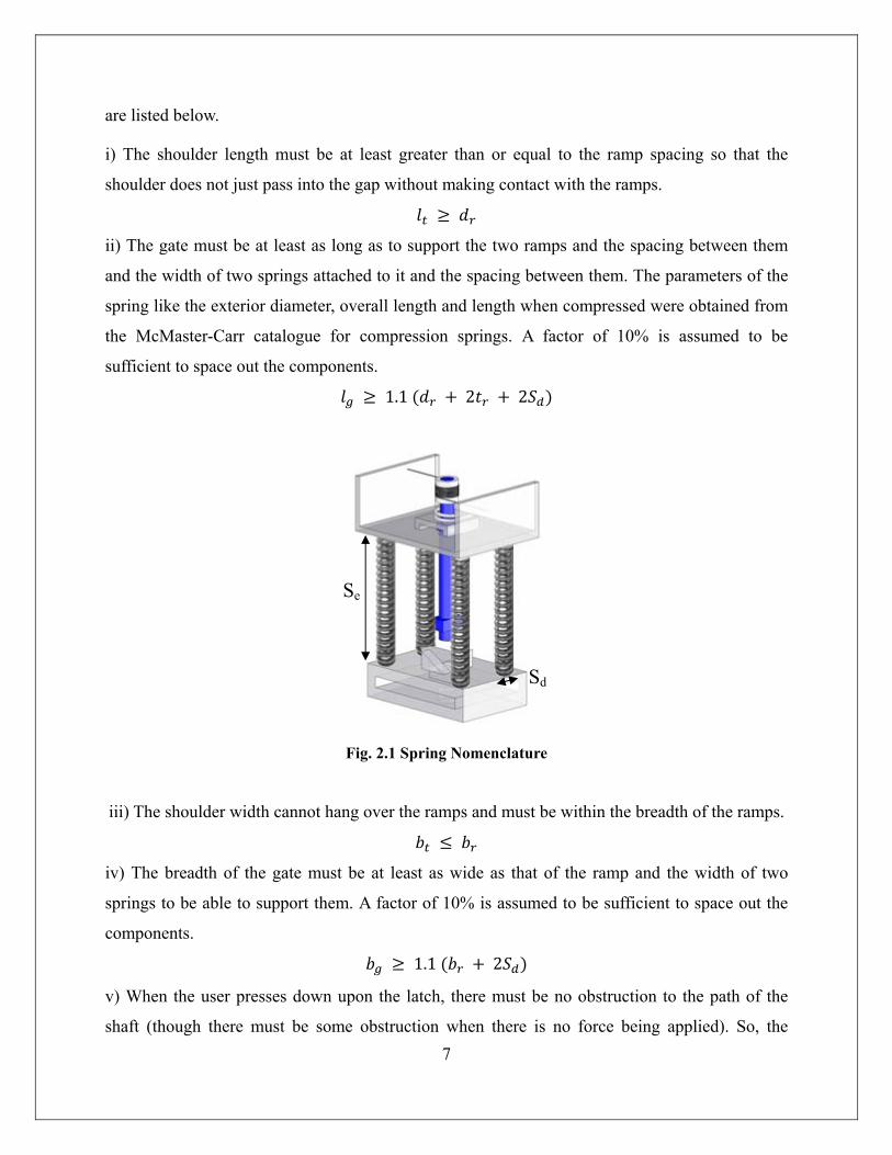
ii) The gate must be at least as long as to support the two ramps and the spacing between them

and the width of two springs attached to it and the spacing between them. The parameters of the

spring like the exterior diameter, overall length and length when compressed were obtained from

the McMaster-Carr catalogue for compression springs. A factor of 10% is assumed to be

sufficient to space out the components.

1.1 2 2

Fig. 2.1 Spring Nomenclature

iii) The shoulder width cannot hang over the ramps and must be within the breadth of the ramps.

iv) The breadth of the gate must be at least as wide as that of the ramp and the width of two

springs to be able to support them. A factor of 10% is assumed to be sufficient to space out the

components.

1.1 2

v) When the user presses down upon the latch, there must be no obstruction to the path of the

shaft (though there must be some obstruction when there is no force being applied). So, the

Sd

Se

8

breadth of the shoulder must be less than the ramp spacing. A factor of 10% is assumed for a

good clearance.

1.1

vi) The gate width must be at least equal to the shoulder length. This is because, when the

shoulder rotates while being inserted into the gate, the shoulder length is along the width of the

gate and the gate must be able to accommodate it.

vii) The breadth of the shoulder must be at least as big as the diameter of the shaft.

viii) During engagement, the shoulder length must be small enough to pass through the ramp

breadth.

ix) The shaft diameter must be smaller than the ramp spacing in order to pass through it without

any contact. A factor of 10% is assumed for a good clearance.

1.1

x) The sum of the height of the shaft and the ramp height when the latch is not engaged, must be

equal to the free length of the springs. This constraint written here for clarity but in the model

execution, it is used to eliminate to decrease the number of variables.

1.05

xi) The shaft height after engaging the latch must be greater than the specified compressed length

of the springs.

xii) The shaft height must be at least as large as to not fit fully inside the gate when the latch is

engaged. So, it must be greater than the sum of the gate thickness and the ramp height.

9

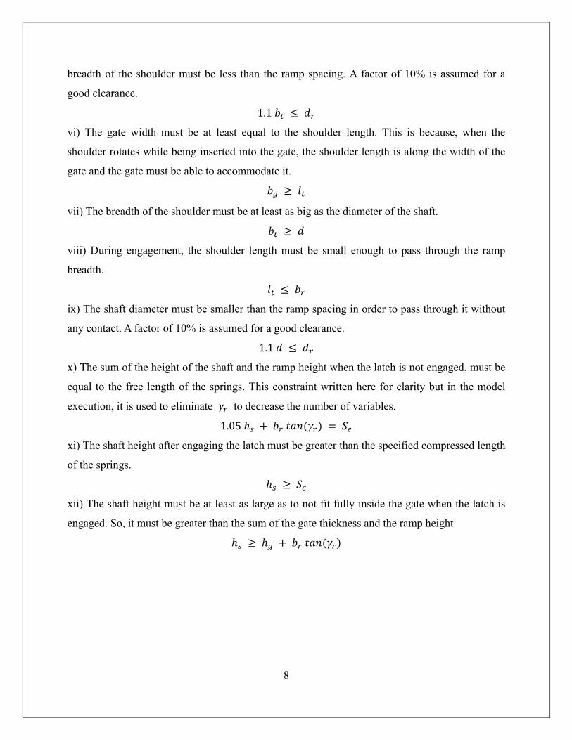
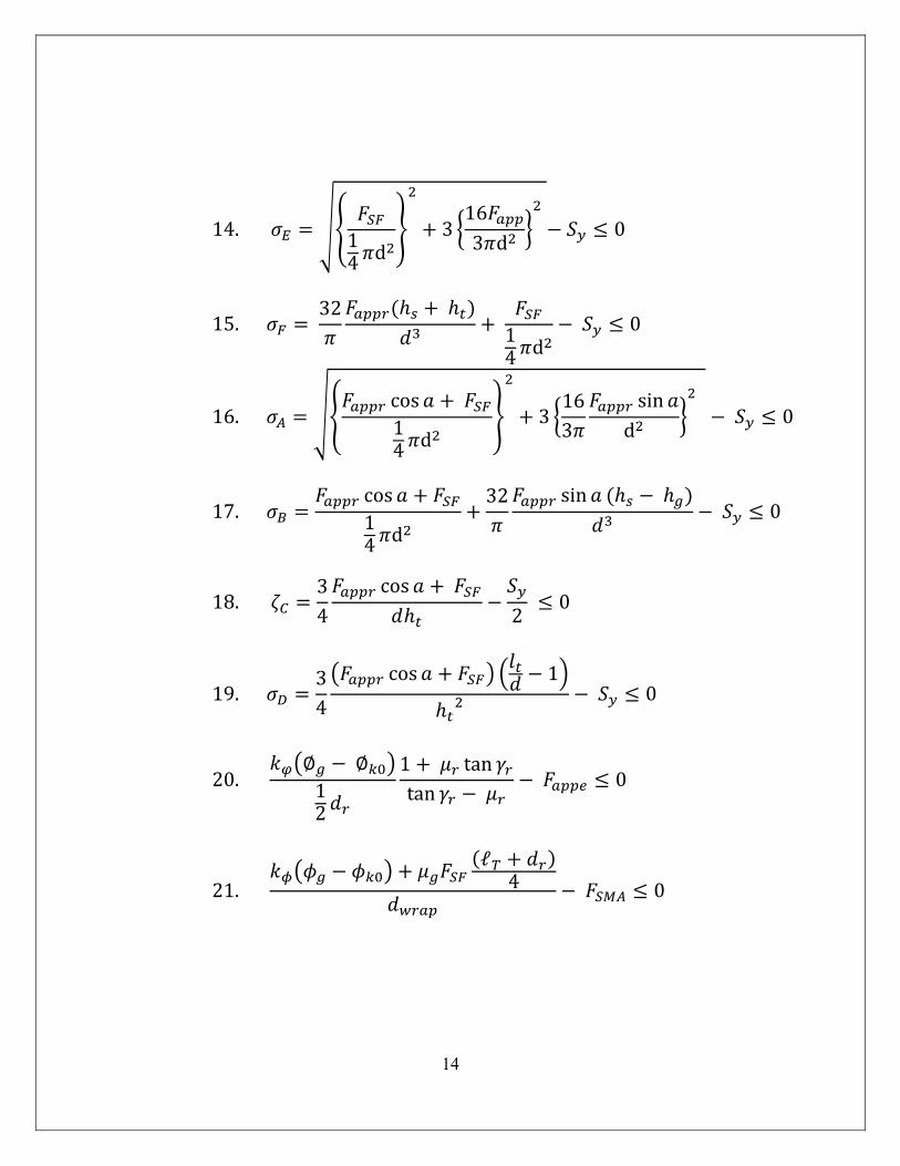
2.2.2.2. Physical Constraints:

Some physical constraints, for the retention stage, based on yield strength and failure

criteria, are described in [1]. These were arrived at by identifying points of maximum von Mises

stress due to axial stress and transverse shear stress in the shaft (point A, Fig. 2.2a), maximum

von Mises stress due to axial and bending stress in the shaft (point B), maximum transverse shear

in the shoulder (datum C-C) and maximum bending stress in the shoulder (point D). These were

identified for case where external force is applied in the plane of the shoulder and the shaft. A

case of normal to shoulder was also analyzed. Points where maximum von Mises stress due to

axial and transverse shear in the shaft act (point E, Fig. 2.2b) and maximum von Mises stress due

to axial and bending stresses in the shoulder act (point F) were identified as critical. These are

summarized in Table 2.1.

Fig. 2.2a: Schematic of the T-latch with a general applied load for the plane of shoulder loading case and

locations of the key stresses

Fig. 2.2b: Free body diagram for normal to shoulder loading of the T.

10

Table 2.1 Stress Constraints

Other constraints arise from the torque requirement in the engagement and release stages.

The moment the user must apply must be greater than the moment offered by the reset spring if

engagement has to occur. This can be summarized as-

12

1

For this to be valid, the denominator of the equation must be greater than zero. This is

also the definition of the coefficient of friction.

0

To reset the latch, the moment from the SMA wire must be greater than the combined

moment of the frictional force between the gate/shoulder and the reset spring.

ℓ4

11

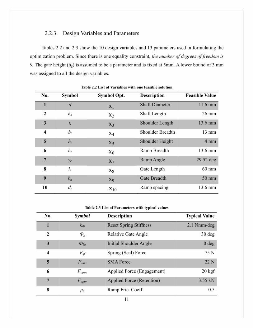
2.2.3. Design Variables and Parameters

Tables 2.2 and 2.3 show the 10 design variables and 13 parameters used in formulating the

optimization problem. Since there is one equality constraint, the number of degrees of freedom is

9. The gate height (hg) is assumed to be a parameter and is fixed at 5mm. A lower bound of 3 mm

was assigned to all the design variables.

Table 2.2 List of Variables with one feasible solution

No. Symbol Symbol Opt. Description Feasible Value

1 d x1 Shaft Diameter 11.6 mm

2 hs x2 Shaft Length 26 mm

3 lt x3 Shoulder Length 13.6 mm

4 bt x4 Shoulder Breadth 13 mm

5 ht x5 Shoulder Height 4 mm

6 br x6 Ramp Breadth 13.6 mm

7 γr x7 Ramp Angle 29.52 deg

8 lg x8 Gate Length 60 mm

9 bg x9 Gate Breadth 50 mm

10 dr x10 Ramp spacing 13.6 mm

Table 2.3 List of Parameters with typical values

No. Symbol Description Typical Value

1 kФ Reset Spring Stiffness 2.1 Nmm/deg

2 Фg Relative Gate Angle 30 deg

3 Фko Initial Shoulder Angle 0 deg

4 Fsf Spring (Seal) Force 75 N

5 Fsma SMA Force 22 N

6 Fappe Applied Force (Engagement) 20 kgf

7 Fappr Applied Force (Retention) 3.55 kN

8 μr Ramp Fric. Coeff. 0.5

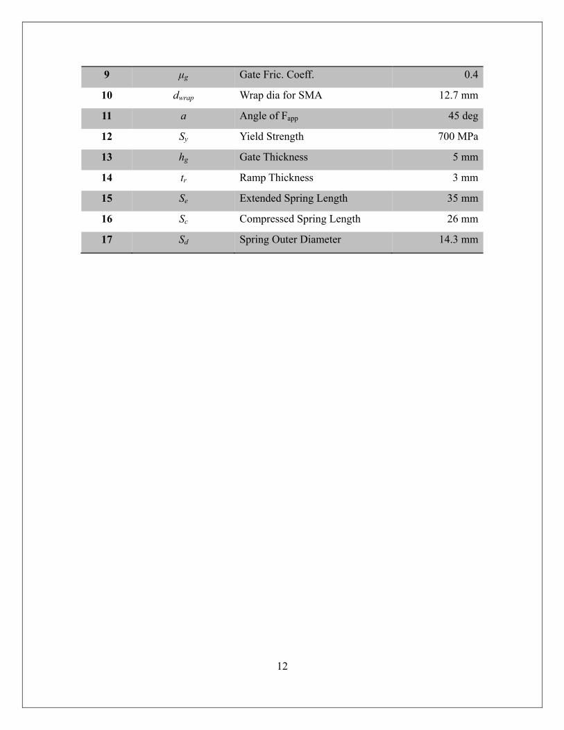
12

9 μg Gate Fric. Coeff. 0.4

10 dwrap Wrap dia for SMA 12.7 mm

11 a Angle of Fapp 45 deg

12 Sy Yield Strength 700 MPa

13 hg Gate Thickness 5 mm

14 tr Ramp Thickness 3 mm

15 Se Extended Spring Length 35 mm

16 Sc Compressed Spring Length 26 mm

17 Sd Spring Outer Diameter 14.3 mm

13

2.2.4. Summary Model The objective function along with the set of constraints is shown below.

Minimize V = 1.05 + + tan + 3

Subject to:

1. 0

2. 1.1 2 2 0

3. 0

4. 1.1 2 0

5. 1.1 0

6. 0

7. 0

8. 0

9. 1.1 0

10. 1.05 0

11. 0

12. 0

13. 0

14

14. 14 d

3163 d

0

15. 32

14 d

0

16. cos 14 d

3163

sind

0

17. cos14 d

32 sin 0

18. 34

cos 2

0

19. 34

cos 1 0

20.

12

1 tantan

0

21. ℓ

4 0

15

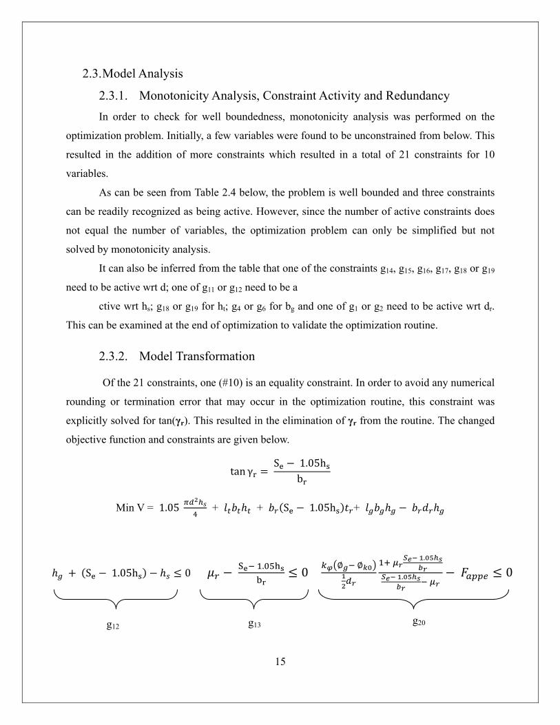
2.3. Model Analysis

2.3.1. Monotonicity Analysis, Constraint Activity and Redundancy In order to check for well boundedness, monotonicity analysis was performed on the

optimization problem. Initially, a few variables were found to be unconstrained from below. This

resulted in the addition of more constraints which resulted in a total of 21 constraints for 10

variables.

As can be seen from Table 2.4 below, the problem is well bounded and three constraints

can be readily recognized as being active. However, since the number of active constraints does

not equal the number of variables, the optimization problem can only be simplified but not

solved by monotonicity analysis.

It can also be inferred from the table that one of the constraints g14, g15, g16, g17, g18 or g19

need to be active wrt d; one of g11 or g12 need to be a

ctive wrt hs; g18 or g19 for ht; g4 or g6 for bg and one of g1 or g2 need to be active wrt dr.

This can be examined at the end of optimization to validate the optimization routine.

2.3.2. Model Transformation

Of the 21 constraints, one (#10) is an equality constraint. In order to avoid any numerical

rounding or termination error that may occur in the optimization routine, this constraint was

explicitly solved for tan(γr). This resulted in the elimination of γr from the routine. The changed

objective function and constraints are given below.

tan γ S 1.05h

b

Min V = 1.05 + + S 1.05h +

S 1.05h 0 S . 0 .

. 0

g12 g13 g20

16

Table 2.4 Monotonicity Analysis

d hs lt bt ht br γr lg bg dr Result

f + U + + + U + + + -

g1 - + Active wrt lt by MPI

g2 - + Active wrt lg, by MPI

g3 + -

g4 + -

g5 + -

g6 + -

g7 + - Active wrt bt by MPI

g8 + -

g9 + -

g11 -

g12 - + +

g13 -

g14 -

g15 - + +

g16 -

g17 - +

g18 - -

g19 - + -

g20 U -

g21 + +

17

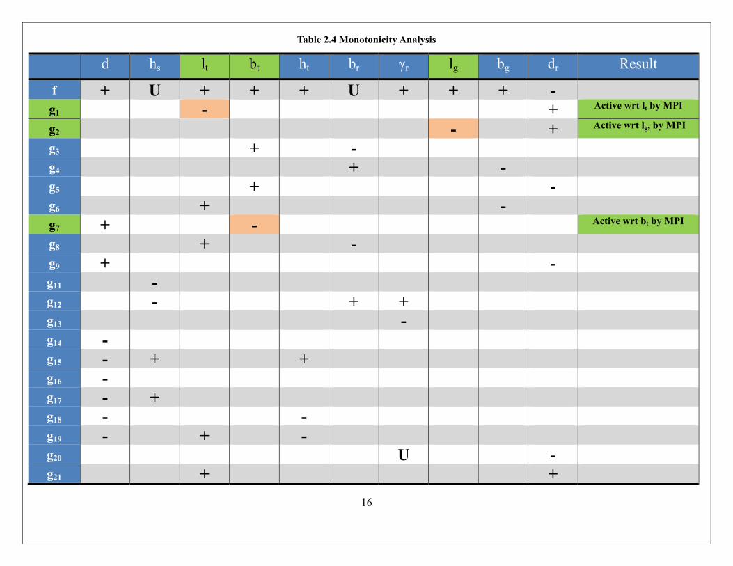
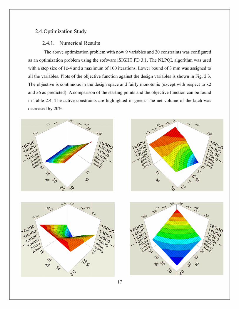
2.4. Optimization Study

2.4.1. Numerical Results The above optimization problem with now 9 variables and 20 constraints was configured

as an optimization problem using the software iSIGHT FD 3.1. The NLPQL algorithm was used

with a step size of 1e-4 and a maximum of 100 iterations. Lower bound of 3 mm was assigned to

all the variables. Plots of the objective function against the design variables is shown in Fig. 2.3.

The objective is continuous in the design space and fairly monotonic (except with respect to x2

and x6 as predicted). A comparison of the starting points and the objective function can be found

in Table 2.4. The active constraints are highlighted in green. The net volume of the latch was

decreased by 20%.

18

Fig. 2.3 Plots showing variation of Objective Function with respect to the variables

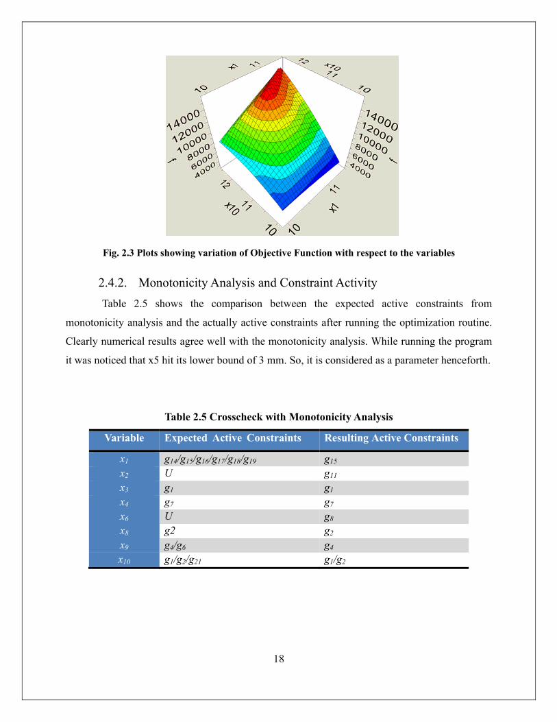
2.4.2. Monotonicity Analysis and Constraint Activity Table 2.5 shows the comparison between the expected active constraints from

monotonicity analysis and the actually active constraints after running the optimization routine.

Clearly numerical results agree well with the monotonicity analysis. While running the program

it was noticed that x5 hit its lower bound of 3 mm. So, it is considered as a parameter henceforth.

Table 2.5 Crosscheck with Monotonicity Analysis

Variable Expected Active Constraints Resulting Active Constraints

x1 g14/g15/g16/g17/g18/g19 g15 x2 U g11 x3 g1 g1 x4 g7 g7 x6 U g8 x8 g2 g2 x9 g4/g6 g4 x10 g1/g2/g21 g1/g2

19

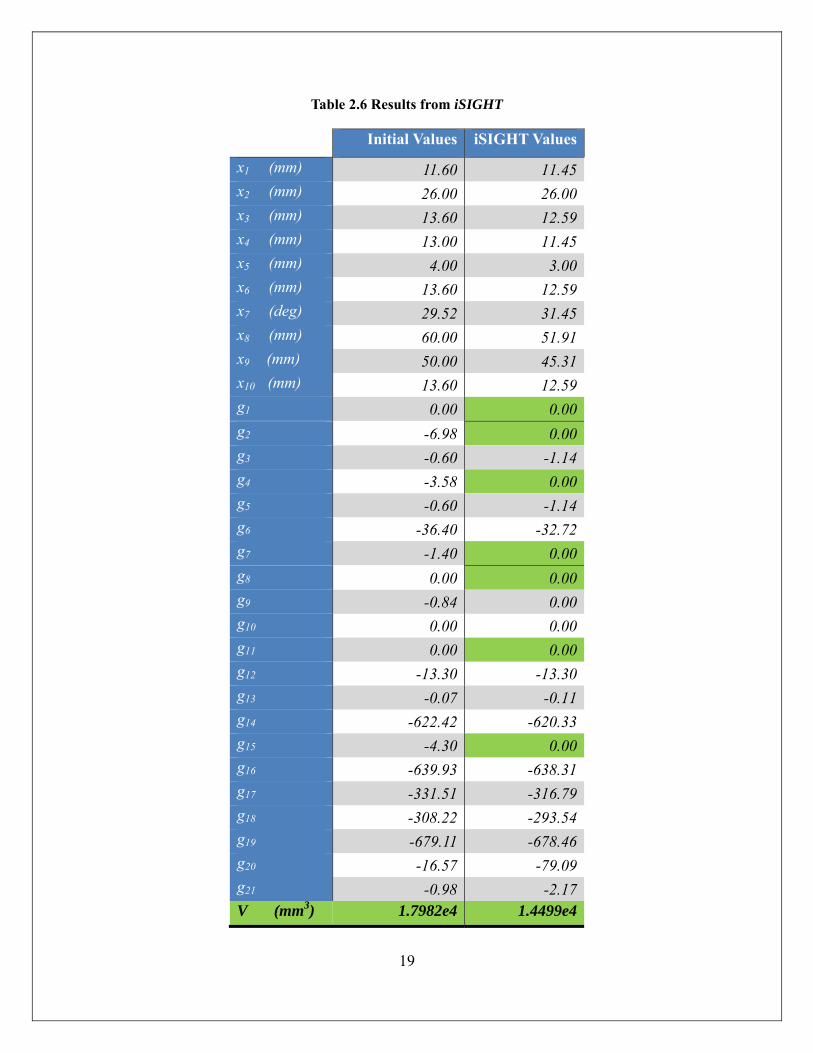
Table 2.6 Results from iSIGHT

Initial Values iSIGHT Values

x1 (mm) 11.60 11.45 x2 (mm) 26.00 26.00 x3 (mm) 13.60 12.59 x4 (mm) 13.00 11.45 x5 (mm) 4.00 3.00 x6 (mm) 13.60 12.59 x7 (deg) 29.52 31.45 x8 (mm) 60.00 51.91 x9 (mm) 50.00 45.31 x10 (mm) 13.60 12.59 g1 0.00 0.00 g2 -6.98 0.00 g3 -0.60 -1.14 g4 -3.58 0.00 g5 -0.60 -1.14 g6 -36.40 -32.72 g7 -1.40 0.00 g8 0.00 0.00 g9 -0.84 0.00 g10 0.00 0.00 g11 0.00 0.00 g12 -13.30 -13.30 g13 -0.07 -0.11 g14 -622.42 -620.33 g15 -4.30 0.00 g16 -639.93 -638.31 g17 -331.51 -316.79 g18 -308.22 -293.54 g19 -679.11 -678.46 g20 -16.57 -79.09 g21 -0.98 -2.17 V (mm3) 1.7982e4 1.4499e4

20

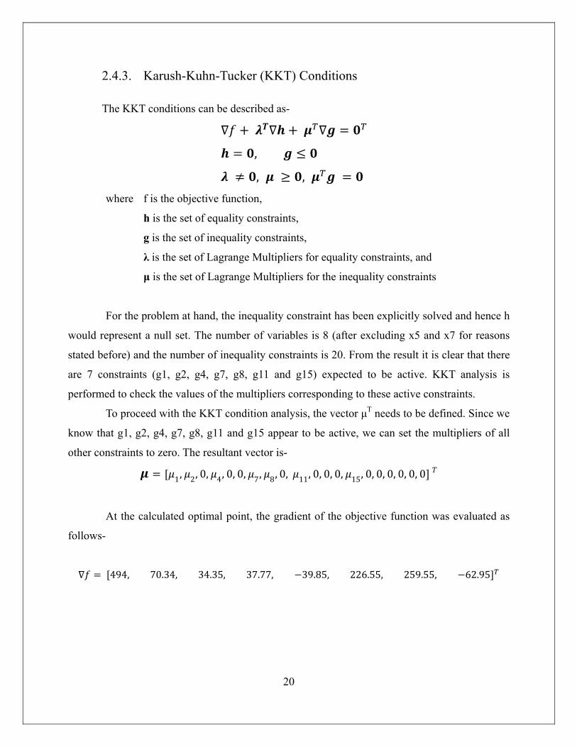
2.4.3. Karush-Kuhn-Tucker (KKT) Conditions

The KKT conditions can be described as-

,

, , where f is the objective function,

h is the set of equality constraints,

g is the set of inequality constraints,

λ is the set of Lagrange Multipliers for equality constraints, and

μ is the set of Lagrange Multipliers for the inequality constraints

For the problem at hand, the inequality constraint has been explicitly solved and hence h

would represent a null set. The number of variables is 8 (after excluding x5 and x7 for reasons

stated before) and the number of inequality constraints is 20. From the result it is clear that there

are 7 constraints (g1, g2, g4, g7, g8, g11 and g15) expected to be active. KKT analysis is

performed to check the values of the multipliers corresponding to these active constraints.

To proceed with the KKT condition analysis, the vector μT needs to be defined. Since we

know that g1, g2, g4, g7, g8, g11 and g15 appear to be active, we can set the multipliers of all

other constraints to zero. The resultant vector is-

1, 2, 0, 4, 0, 0, 7, 8, 0, 11, 0, 0, 0, 15, 0, 0, 0, 0, 0, 0

At the calculated optimal point, the gradient of the objective function was evaluated as

follows-

494, 70.34, 34.35, 37.77, 39.85, 226.55, 259.55, 62.95

21

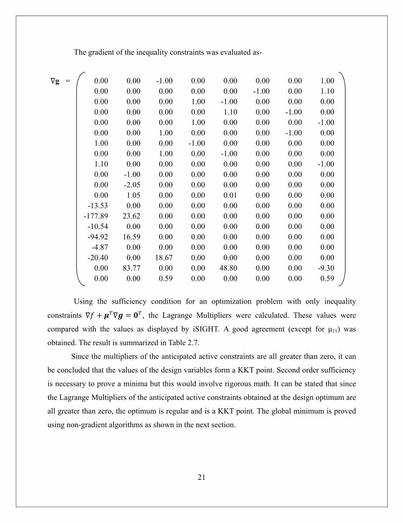
The gradient of the inequality constraints was evaluated as-

g = 0.00 0.00 -1.00 0.00 0.00 0.00 0.00 1.000.00 0.00 0.00 0.00 0.00 -1.00 0.00 1.100.00 0.00 0.00 1.00 -1.00 0.00 0.00 0.000.00 0.00 0.00 0.00 1.10 0.00 -1.00 0.000.00 0.00 0.00 1.00 0.00 0.00 0.00 -1.000.00 0.00 1.00 0.00 0.00 0.00 -1.00 0.001.00 0.00 0.00 -1.00 0.00 0.00 0.00 0.000.00 0.00 1.00 0.00 -1.00 0.00 0.00 0.001.10 0.00 0.00 0.00 0.00 0.00 0.00 -1.000.00 -1.00 0.00 0.00 0.00 0.00 0.00 0.000.00 -2.05 0.00 0.00 0.00 0.00 0.00 0.000.00 1.05 0.00 0.00 0.01 0.00 0.00 0.00

-13.53 0.00 0.00 0.00 0.00 0.00 0.00 0.00-177.89 23.62 0.00 0.00 0.00 0.00 0.00 0.00-10.54 0.00 0.00 0.00 0.00 0.00 0.00 0.00-94.92 16.59 0.00 0.00 0.00 0.00 0.00 0.00-4.87 0.00 0.00 0.00 0.00 0.00 0.00 0.00

-20.40 0.00 18.67 0.00 0.00 0.00 0.00 0.000.00 83.77 0.00 0.00 48.80 0.00 0.00 -9.300.00 0.00 0.59 0.00 0.00 0.00 0.00 0.59

Using the sufficiency condition for an optimization problem with only inequality

constraints , the Lagrange Multipliers were calculated. These values were

compared with the values as displayed by iSIGHT. A good agreement (except for μ11) was

obtained. The result is summarized in Table 2.7.

Since the multipliers of the anticipated active constraints are all greater than zero, it can

be concluded that the values of the design variables form a KKT point. Second order sufficiency

is necessary to prove a minima but this would involve rigorous math. It can be stated that since

the Lagrange Multipliers of the anticipated active constraints obtained at the design optimum are

all greater than zero, the optimum is regular and is a KKT point. The global minimum is proved

using non-gradient algorithms as shown in the next section.

22

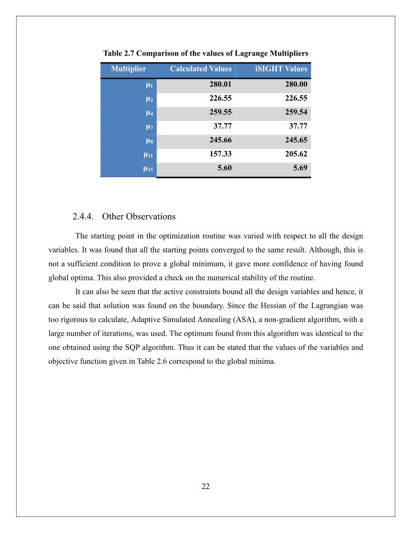
Table 2.7 Comparison of the values of Lagrange Multipliers

Multiplier Calculated Values iSIGHT Values

μ1 280.01 280.00

μ2 226.55 226.55

μ4 259.55 259.54

μ7 37.77 37.77

μ8 245.66 245.65

μ11 157.33 205.62

μ15 5.60 5.69

2.4.4. Other Observations

The starting point in the optimization routine was varied with respect to all the design

variables. It was found that all the starting points converged to the same result. Although, this is

not a sufficient condition to prove a global minimum, it gave more confidence of having found

global optima. This also provided a check on the numerical stability of the routine.

It can also be seen that the active constraints bound all the design variables and hence, it

can be said that solution was found on the boundary. Since the Hessian of the Lagrangian was

too rigorous to calculate, Adaptive Simulated Annealing (ASA), a non-gradient algorithm, with a

large number of iterations, was used. The optimum found from this algorithm was identical to the

one obtained using the SQP algorithm. Thus it can be stated that the values of the variables and

objective function given in Table 2.6 correspond to the global minima.

23

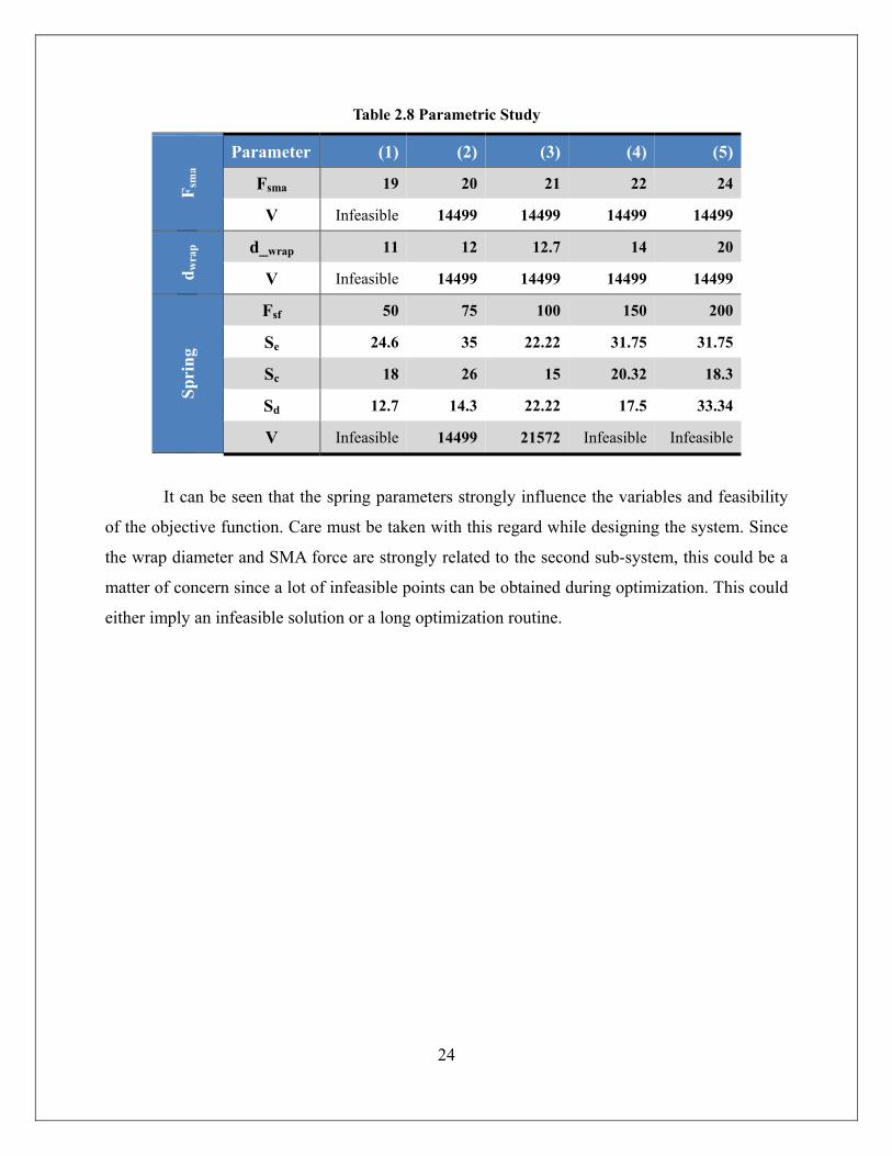
2.5. Parametric Study

The design of the T-Latch is inherently linked to the SMA sub-system. So, it would be

interesting to study how the parameters like Fsma and wrap diameter affect the objective function.

2.5.1. SMA force The variation of the net volume of the latch with the force of SMA wire is show in Table

2.8. It is noted that Fsma appears in a constraint that is not active. So Fsma only defines the feasible

region and when it remains within limits, it will not affect the objective function. This is

observed from the table where for values of Fsma about 22 N, the value of net volume of

packaging remains constant. However, at about 19 N infeasible solutions are obtained. This

shows that a very narrow feasible domain exists with respect to the force of the SMA wire. A

minimum force of 22 N assumed as a parameter, however, would be valid.

2.5.2. Wrap Diameter The wrap diameter also figures in an inactive constraint. Therefore, while it will not

affect the objective function when it is within a range, outside this range, it will have an

influence on the design variables and hence the objective function. Like the SMA force, the

range is very narrow on one side of the presently assumed value of 12.7 mm. This is shown in

Table 2.8.

2.5.3. Spring (Seal) Force It was has been shown that several constraints containing parameters pertaining to the

seal spring strongly influence the objective function. So it would indeed be interesting to see how

the objective changes with the spring force. The range of the spring force, overall length,

compressed length and outer diameter was obtained from the McMaster-Carr catalogue. The

results are shown in Table 2.8.

24

Table 2.8 Parametric Study

F sm

a

Parameter (1) (2) (3) (4) (5)

Fsma 19 20 21 22 24

V Infeasible 14499 14499 14499 14499

d wra

p d_wrap 11 12 12.7 14 20

V Infeasible 14499 14499 14499 14499

Spri

ng

Fsf 50 75 100 150 200

Se 24.6 35 22.22 31.75 31.75

Sc 18 26 15 20.32 18.3

Sd 12.7 14.3 22.22 17.5 33.34

V Infeasible 14499 21572 Infeasible Infeasible

It can be seen that the spring parameters strongly influence the variables and feasibility

of the objective function. Care must be taken with this regard while designing the system. Since

the wrap diameter and SMA force are strongly related to the second sub-system, this could be a

matter of concern since a lot of infeasible points can be obtained during optimization. This could

either imply an infeasible solution or a long optimization routine.

25

2.6. Discussion of Results

Numerical and analytical results using monotonicity analysis and the KKT conditions

indicate that the optimum obtained is indeed a stationary point and could be global. The optimal

solution gives a volume of about 15 cm3. This makes physical sense as one can picture a device

built to this overall dimension. The dimensions of the device mentioned in [1] support this

statement. In the optimized dimensions, the volume of the latch was decreased by about 20%.

It is noted that most of the active constraints are practical constraints. This means that

the design is determined more by geometry rather than stress limitations. That is, given precise

manufacturing methods to attain smaller dimensions and given springs of desired dimensions,

one could further reduce the net volume of the device while not violating the stress constraints.

So, if there is a way, for example, to reduce the spring length and outer diameter while still

maintaining the required seal force, a better solution can be obtained.

The tolerance on the designs to accommodate assembly misalignments, 10% of the base

for example, was only an estimate. However, it strongly influences the constraints (active g2 and

g4 for example). The tolerance could be reduced or increased depending on the availability of

precise assembly or packaging space. This mimics the physical design process where parts are

built to dimensions that tolerate small variations in assembly.

As noted in the parametric study, the tolerance of the feasibility of this subsystem

relative to the variables of the second sub-system namely the SMA Force and the wrap diameter

is very poor. This could dictate the feasible domain of the design in the system integration model.

On the flip side, the shoulder length and the ramp spacing are parameters for the second

subsystem. Depending on whether the constraints involved in that system are active or not, these

could influence the system optima. This means that the two subsystems are essentially coupled

and neither gets preference over the other while running the system optimization routine.

26

3. Spool-Packaged SMA Wire Actuator (Subsystem 2) : WonHee Kim

Shape Memory Alloy actuators are very attractive for many applications because of their

high energy density, reduced size and weight, robust performance, and simple architecture.

Especially SMA wire is more advantageous to be implemented because of its well-developed

manufacturing and quality control, actuation with simple electrical control circuit, and fast

heating and cooling speed. However, to ensure the enough strokes for a practical application,

long lengths of SMA wire should be stored in a small package. To address this packaging

challenge, a spooling technique that wraps portions of the wire around mandrels to reduce the

packaged length had been used in applications such as active latches [1], pedestrian protection

[3], vibration suppression in hand-held arms [4], and biomedical applications [5, 6]. But, this

technique does sacrifice some performance due to accumulating friction between the SMA wire

and mandrel. To understand the output motion and limitation of this technique, an analytical

model for linear spooled SMA actuators had been studied by Redmond et al. [2, 7, 8]. In this

study, we will use this analytical model to optimize the design of the SMA wire actuator.

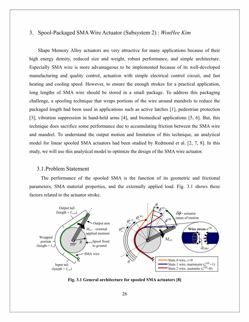
3.1. Problem Statement The performance of the spooled SMA is the function of its geometric and frictional

parameters, SMA material properties, and the externally applied load. Fig. 3.1 shows these

factors related to the actuator stroke.

Fig. 3.1 General architecture for spooled SMA actuators [8]

27

Because of the non-linear behavior of the SMA wire, the performance of the SMA wire

actuator is not linearly proportional to the geometry of the SMA wire actuator design, the

diameter, length, and the free clearance, even with the straight wire actuator without spooling

mechanism. With the spooling mechanism, there are more factors which affect the performance

of the SMA wire actuator; such as the diameter of the spool, wrap angle, and the length of the

input tail. The goal of this study is to optimize the spool-packaged SMA wire actuator design for

the minimum input power usage.

3.2. Mathematical Model

3.2.1. Objective function As mentioned in the problem statement, the object of this study is to minimize the input

power for the phase transformation of the SMA wire from the martensite phase to the austenite

phase, and the input power is determined by the diameter of the SMA wire dSMA and the total

length of the SMA wire ℓtotal.

ℓ 2.527 10.

5.519 10.

(3.1)

R I2

3.2.2. Constraints The SMA wire actuator should generate the enough force to release the T-latch, and the

required force is determined by the stiffness of the reset spring and the friction between the T of

the latch and the engagement ramp.

, 0ℓ

(3.2)

The stroke of the SMA wire actuator should be bigger than the required stroke which can

release the T from the engagement ramp. And this stroke should be translated to the rotation.

3.3

The force of the SMA wire can be calculated by the stress of the SMA wire and the cross

28

sectional area of the wire. The stress of the wire can be obtained by the constitutive model of the

stress-strain relationship of the wire.

, 0 , 0 3.4

Without the spooling mechanism, the stroke of the SMA wire can be obtained by the

changes of the equilibrium state between the SMA wire and the reset spring. And the equilibrium

state can be obtained graphically with the constitutive model of the stress-strain curve. The

stroke can be calculated by multiplying the original length with the difference between the

austenite strain and the martensite strain. However, because of the friction between the SMA

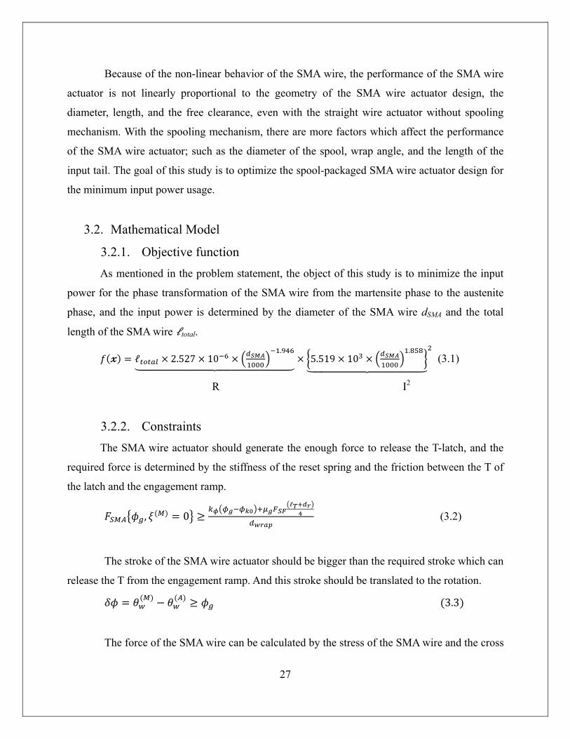
wire and the spool, we need to use the modification of the strain. Fig. 3.2 shows the effect of the

friction in a differential element.

Fig. 3.2 Free body diagram of a differential element of SMA in sliding contact with the spool [2]

Equation (3.5) and (3.6) are the model of the stress at the angle under the martensite

and the austenite respectively.

(3.5)

(3.6)

As the strain of the SMA wire under the certain stress can be obtained by the constitutive

model of the stress-strain relationship, we can get the modified strain with the equation (3.7) and

(3.8).

(3.7)

29

(3.8)

Stress at the tail is determined by the counter force from the T-Latch.

ℓ

(3.9)

ℓ

(3.10)

Relating the un-deformed length of each half of the SMA wire to the strain profiles of

the martensite and austenite wires yields the compatibility equations for each state.

ℓ 1 ℓ (3.11)

ℓ 1 ℓ (3.12)

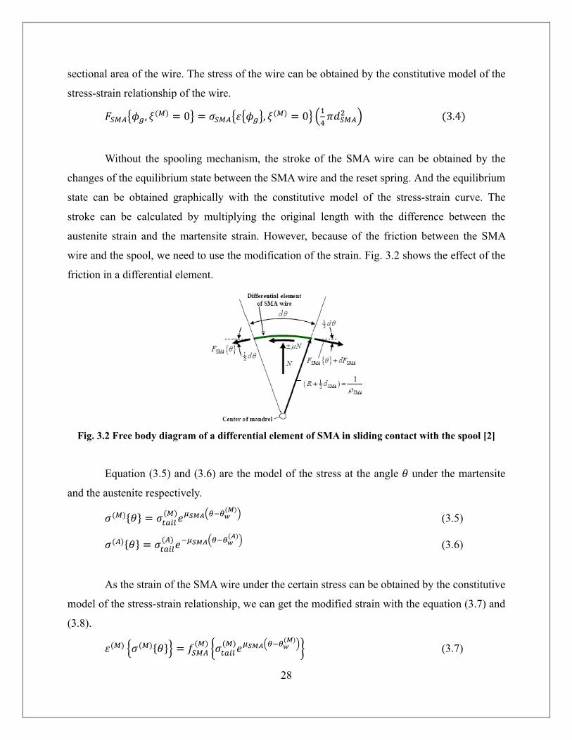
The constitutive model of the stress-strain of the SMA wire can be obtained from the

experiment data by curve fitting. We will use the constitutive model of the previous study [8].

4.6 10 3.0 10 6.8 10 21.4 (3.13)

72.5 10 (3.14)

Fig. 3.3 Stress-strain model for material behavior [8]

30

One of the limitations of the SMA is that it shows the shakedown effect. To avoid the

shakedown effect of the SMA wire actuator, the maximum stress should be limited within

250MPa ( ), and the maximum strain should be less than 4% [9].

, 0 3.15

0.04 (3.16)

To connect the SMA wire to the spool, minimum length of the wrap length should be

ensured. In addition to the minimum length of the wrap length, the tail length must be smaller

than the total length of the SMA wire. To ensure these conditions, instead of the tail length we

can introduce the ratio between the tail length and the total length.

ℓ ℓℓ

(3.17)

0 ℓ 0.7 (3.18)

The SMA wire is available as a commercial product with the 6, 8, 10, 12, 15, and 20 mil.

For the optimization study, we will consider the diameter of the SMA wire as a continuous

variable.

6 20 (3.19)

The diameter of the spool should be bigger than the diameter of the shaft.

10 (3.20)

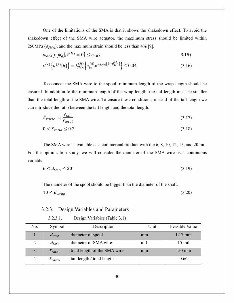
3.2.3. Design Variables and Parameters 3.2.3.1. Design Variables (Table 3.1)

No. Symbol Description Unit Feasible Value

1 dwrap diameter of spool mm 12.7 mm

2 dSMA diameter of SMA wire mil 15 mil

3 ℓ total length of the SMA wire mm 150 mm

4 ℓ tail length / total length 0.66

31

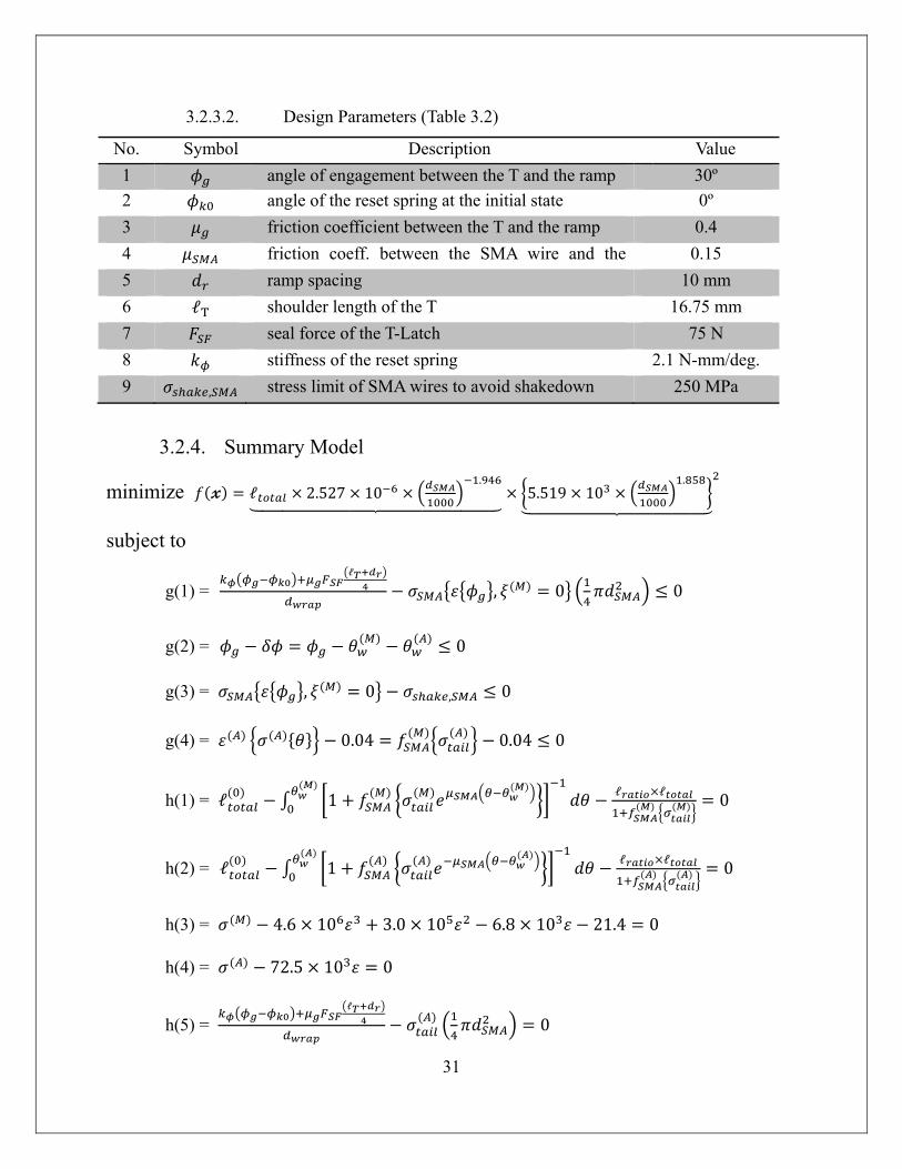
3.2.3.2. Design Parameters (Table 3.2)

No. Symbol Description Value 1 angle of engagement between the T and the ramp 30º 2 angle of the reset spring at the initial state 0º 3 friction coefficient between the T and the ramp 0.4 4 friction coeff. between the SMA wire and the 0.15 5 ramp spacing 10 mm 6 ℓT shoulder length of the T 16.75 mm 7 seal force of the T-Latch 75 N 8 stiffness of the reset spring 2.1 N-mm/deg. 9 , stress limit of SMA wires to avoid shakedown 250 MPa

3.2.4. Summary Model

minimize ℓ 2.527 10.

5.519 10.

subject to

g(1) = ℓ

, 0 0

g(2) = 0

g(3) = , 0 , 0

g(4) = 0.04 0.04 0

h(1) = ℓ 1 ℓ ℓ 0

h(2) = ℓ 1 ℓ ℓ 0

h(3) = 4.6 10 3.0 10 6.8 10 21.4 0

h(4) = 72.5 10 0

h(5) = ℓ

0

32

h(6) = ℓ

0

set constraints

0 ℓ 0.7, 6 20, 10

3.3. Model Analysis The objective function of the model contains two design variables, and the function is

monotonic with respect to both of them.

ℓ ,

The inequality constraint g(1) and the equality constraint h(5) are redundant constraints, and

g(1) should be active constraint.

and can be calculated from the equality constraints h(1) and h(2) respectively.

ℓ , ℓ , ,

ℓ , ℓ , ,

The values of and are not monotonic with respect to the variables, so it is hard to do

the monotonicity analysis with the inequality constraint g(2).

and are the inverse functions of the function h(3) and h(4), and is

monotonic with respect to . And is derived from the equality constraint h(5).

,

However, because of the relation between other variables, it is hard to predict the activity of g(4).

3.4. Optimization Study

3.4.1. Optimization Results

Just as stated in the section 3.4, the complexity the and makes this model

very difficult to calculate. To address this problem, iSight-FD is used with MATLAB code with

Sequential Quadratic Programming (SQP). To verify the results from the SQP, Simulated

Annealing and the Genetic Algorithm also had been used.

33

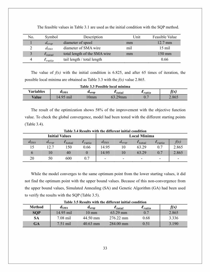
The feasible values in Table 3.1 are used as the initial condition with the SQP method.

No. Symbol Description Unit Feasible Value 1 dwrap diameter of spool mm 12.7 mm 2 dSMA diameter of SMA wire mil 15 mil 3 ℓ total length of the SMA wire mm 150 mm 4 ℓ tail length / total length 0.66

The value of f(x) with the initial condition is 6.825, and after 65 times of iteration, the

possible local minima are obtained as Table 3.3 with the f(x) value 2.865.

Table 3.3 Possible local minima Variables dSMA dwrap f(x)

Value 14.95 mil 10mm 63.29mm 0.7 2.865

The result of the optimization shows 58% of the improvement with the objective function

value. To check the global convergence, model had been tested with the different starting points

(Table 3.4).

Table 3.4 Results with the different initial condition Initial Values Local Minima

dSMA dwrap ℓ ℓ dSMA dwrap ℓ ℓ f(x) 15 12.7 150 0.66 14.95 10 63.29 0.7 2.865 6 10 40 0 14.95 10 63.29 0.7 2.865 20 50 600 0.7 - - - - -

While the model converges to the same optimum point from the lower starting values, it did

not find the optimum point with the upper bound values. Because of this non-convergence from

the upper bound values, Simulated Annealing (SA) and Genetic Algorithm (GA) had been used

to verify the results with the SQP (Table 3.5).

Table 3.5 Results with the different initial condition

Method dSMA dwrap f(x) SQP 14.95 mil 10 mm 63.29 mm 0.7 2.865 SA 7.08 mil 44.50 mm 276.22 mm 0.68 3.336 GA 7.51 mil 40.63 mm 284.00 mm 0.51 3.190

34

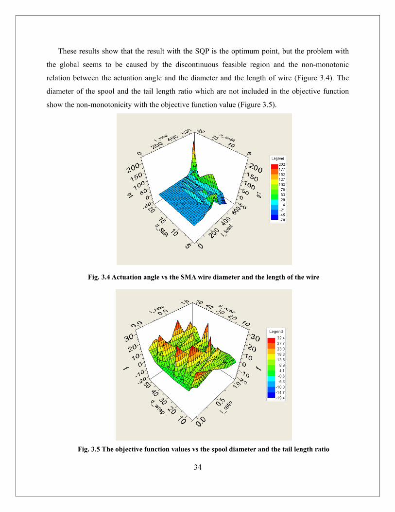
These results show that the result with the SQP is the optimum point, but the problem with

the global seems to be caused by the discontinuous feasible region and the non-monotonic

relation between the actuation angle and the diameter and the length of wire (Figure 3.4). The

diameter of the spool and the tail length ratio which are not included in the objective function

show the non-monotonicity with the objective function value (Figure 3.5).

Fig. 3.4 Actuation angle vs the SMA wire diameter and the length of the wire

Fig. 3.5 The objective function values vs the spool diameter and the tail length ratio

35

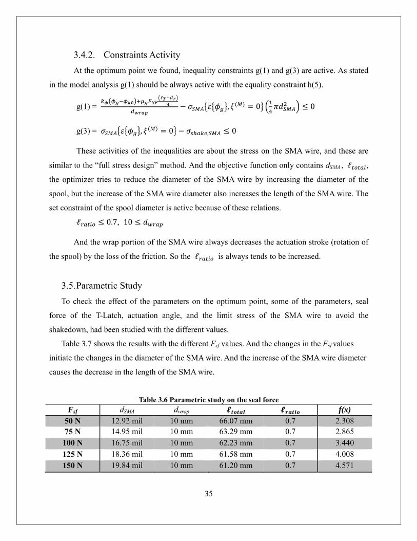
3.4.2. Constraints Activity At the optimum point we found, inequality constraints g(1) and g(3) are active. As stated

in the model analysis g(1) should be always active with the equality constraint h(5).

g(1) = ℓ

, 0 0

g(3) = , 0 , 0

These activities of the inequalities are about the stress on the SMA wire, and these are

similar to the “full stress design” method. And the objective function only contains dSMA , ℓ ,

the optimizer tries to reduce the diameter of the SMA wire by increasing the diameter of the

spool, but the increase of the SMA wire diameter also increases the length of the SMA wire. The

set constraint of the spool diameter is active because of these relations.

ℓ 0.7, 10

And the wrap portion of the SMA wire always decreases the actuation stroke (rotation of

the spool) by the loss of the friction. So the ℓ is always tends to be increased.

3.5. Parametric Study To check the effect of the parameters on the optimum point, some of the parameters, seal

force of the T-Latch, actuation angle, and the limit stress of the SMA wire to avoid the

shakedown, had been studied with the different values. Table 3.7 shows the results with the different Fsf values. And the changes in the Fsf values

initiate the changes in the diameter of the SMA wire. And the increase of the SMA wire diameter

causes the decrease in the length of the SMA wire.

Table 3.6 Parametric study on the seal force Fsf dSMA dwrap f(x)

50 N 12.92 mil 10 mm 66.07 mm 0.7 2.308 75 N 14.95 mil 10 mm 63.29 mm 0.7 2.865 100 N 16.75 mil 10 mm 62.23 mm 0.7 3.440 125 N 18.36 mil 10 mm 61.58 mm 0.7 4.008 150 N 19.84 mil 10 mm 61.20 mm 0.7 4.571

36

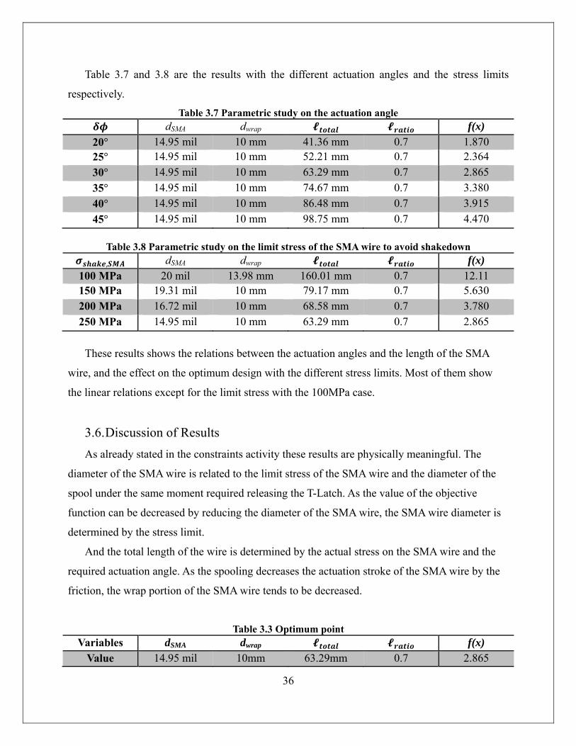
Table 3.7 and 3.8 are the results with the different actuation angles and the stress limits

respectively.

Table 3.7 Parametric study on the actuation angle

dSMA dwrap f(x) 20° 14.95 mil 10 mm 41.36 mm 0.7 1.870 25° 14.95 mil 10 mm 52.21 mm 0.7 2.364 30° 14.95 mil 10 mm 63.29 mm 0.7 2.865 35° 14.95 mil 10 mm 74.67 mm 0.7 3.380 40° 14.95 mil 10 mm 86.48 mm 0.7 3.915 45° 14.95 mil 10 mm 98.75 mm 0.7 4.470

Table 3.8 Parametric study on the limit stress of the SMA wire to avoid shakedown

, dSMA dwrap f(x) 100 MPa 20 mil 13.98 mm 160.01 mm 0.7 12.11 150 MPa 19.31 mil 10 mm 79.17 mm 0.7 5.630 200 MPa 16.72 mil 10 mm 68.58 mm 0.7 3.780 250 MPa 14.95 mil 10 mm 63.29 mm 0.7 2.865

These results shows the relations between the actuation angles and the length of the SMA

wire, and the effect on the optimum design with the different stress limits. Most of them show

the linear relations except for the limit stress with the 100MPa case.

3.6. Discussion of Results As already stated in the constraints activity these results are physically meaningful. The

diameter of the SMA wire is related to the limit stress of the SMA wire and the diameter of the

spool under the same moment required releasing the T-Latch. As the value of the objective

function can be decreased by reducing the diameter of the SMA wire, the SMA wire diameter is

determined by the stress limit.

And the total length of the wire is determined by the actual stress on the SMA wire and the

required actuation angle. As the spooling decreases the actuation stroke of the SMA wire by the

friction, the wrap portion of the SMA wire tends to be decreased.

Table 3.3 Optimum point Variables dSMA dwrap f(x)

Value 14.95 mil 10mm 63.29mm 0.7 2.865

37

Depends on the parameters of the model such as the seal force, the actuation angle, and the

stress limit of the SMA wire, the optimum point can be changed. Particularly the stress limit can

change the activity of the constraint. As the many of the active constraints are based on the

design decision, they should be determined carefully.

38

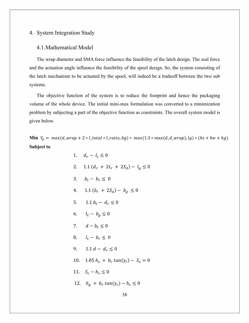
4. System Integration Study

4.1. Mathematical Model

The wrap diameter and SMA force influence the feasibility of the latch design. The seal force

and the actuation angle influence the feasibility of the spool design. So, the system consisting of

the latch mechanism to be actuated by the spool, will indeed be a tradeoff between the two sub

systems.

The objective function of the system is to reduce the footprint and hence the packaging

volume of the whole device. The initial mini-max formulation was converted to a minimization

problem by subjecting a part of the objective function as constraints. The overall system model is

given below.

Min _ 2 _ _ , 1.3 , _ ,

Subject to

1. 0

2. 1.1 2 2 0

3. 0

4. 1.1 2 0

5. 1.1 0

6. 0

7. 0

8. 0

9. 1.1 0

10. 1.05 0

11. 0

12. 0

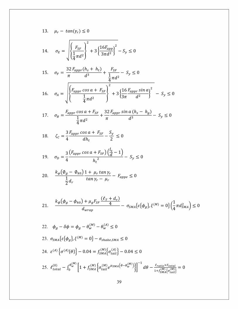
39

13. 0

14. 14

3163 0

15. 32

14

0

16.

14

3163 0

17. 14

32 0

18. 34

2 0

19. 34

1 0

20.

12

1 0

21. ℓ

4 , 014 0

22. 0

23. , 0 , 0

24. 0.04 0.04 0

25. ℓ 1 ℓ ℓ 0

40

26. ℓ 1 ℓ ℓ 0

27. 4.6 10 3.0 10 6.8 10 21.4 0

28. 72.5 10 0

28. ℓ

0

30. ℓ

0

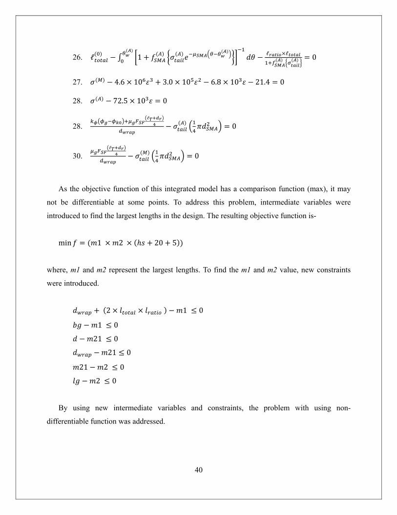
As the objective function of this integrated model has a comparison function (max), it may

not be differentiable at some points. To address this problem, intermediate variables were

introduced to find the largest lengths in the design. The resulting objective function is-

min 1 2 20 5

where, m1 and m2 represent the largest lengths. To find the m1 and m2 value, new constraints

were introduced.

2 1 0

1 0

21 0

21 0

21 2 0

2 0

By using new intermediate variables and constraints, the problem with using non-

differentiable function was addressed.

41

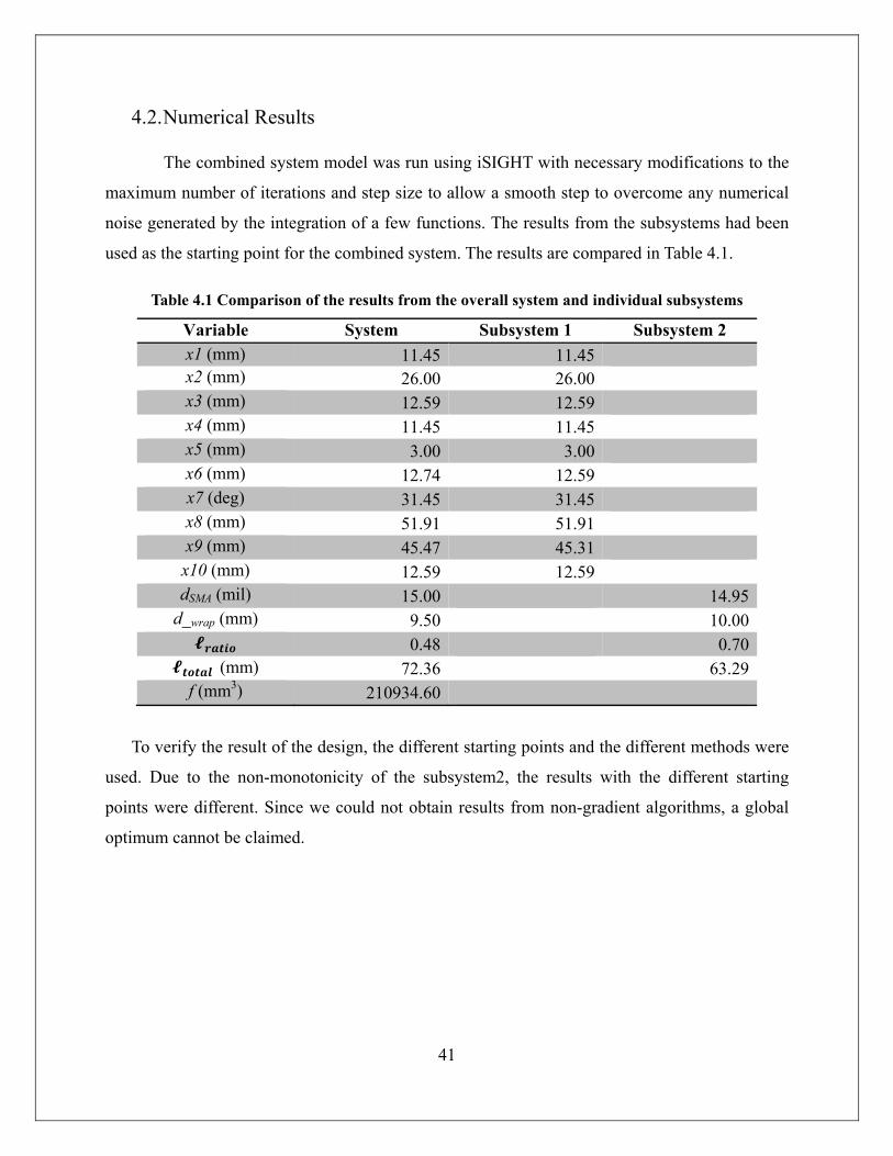
4.2. Numerical Results

The combined system model was run using iSIGHT with necessary modifications to the

maximum number of iterations and step size to allow a smooth step to overcome any numerical

noise generated by the integration of a few functions. The results from the subsystems had been

used as the starting point for the combined system. The results are compared in Table 4.1.

Table 4.1 Comparison of the results from the overall system and individual subsystems

Variable System Subsystem 1 Subsystem 2 x1 (mm) 11.45 11.45x2 (mm) 26.00 26.00x3 (mm) 12.59 12.59x4 (mm) 11.45 11.45x5 (mm) 3.00 3.00x6 (mm) 12.74 12.59x7 (deg) 31.45 31.45x8 (mm) 51.91 51.91x9 (mm) 45.47 45.31x10 (mm) 12.59 12.59dSMA (mil) 15.00 14.95

d_wrap (mm) 9.50 10.00 0.48 0.70

(mm) 72.36 63.29f (mm3) 210934.60

To verify the result of the design, the different starting points and the different methods were

used. Due to the non-monotonicity of the subsystem2, the results with the different starting

points were different. Since we could not obtain results from non-gradient algorithms, a global

optimum cannot be claimed.

42

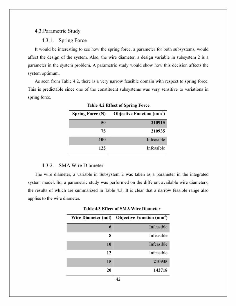
4.3. Parametric Study

4.3.1. Spring Force It would be interesting to see how the spring force, a parameter for both subsystems, would

affect the design of the system. Also, the wire diameter, a design variable in subsystem 2 is a

parameter in the system problem. A parametric study would show how this decision affects the

system optimum.

As seen from Table 4.2, there is a very narrow feasible domain with respect to spring force.

This is predictable since one of the constituent subsystems was very sensitive to variations in

spring force.

Table 4.2 Effect of Spring Force

Spring Force (N) Objective Function (mm3)

50 210915

75 210935

100 Infeasible

125 Infeasible

4.3.2. SMA Wire Diameter The wire diameter, a variable in Subsystem 2 was taken as a parameter in the integrated

system model. So, a parametric study was performed on the different available wire diameters,

the results of which are summarized in Table 4.3. It is clear that a narrow feasible range also

applies to the wire diameter.

Table 4.3 Effect of SMA Wire Diameter

Wire Diameter (mil) Objective Function (mm3)

6 Infeasible

8 Infeasible

10 Infeasible

12 Infeasible

15 210935

20 142718

43

4.4. Discussion of Results The result gives the volume of packaging of the device is greater than the net volume of the

‘T’ alone. This shows a strong correlation between the two subsystems. If the parameters of the

subsystems could be dynamically changed as the system integration model changes, the

individual subsystems would benefit.

More investigation is necessary to understand why the non-gradient based algorithms could

not arrive at a feasible point even after a considerable amount of running time. In other words,

the narrow feasible region of the problem remains to be analyzed.

The total footprint of the device is about 211 cm3. This is the space under the hood of the car

required to support the device.

44

5. Acknowledgments We would like to thank the Smart Materials and Structures group at the University of

Michigan, particularly Prof. Diann Brei and John A Redmond for their assistance in framing the

optimization problem for both the subsystems. We are indebted to Kwang Jae Lee who was

always ready to help us out with specific issues regarding modeling and using iSIGHT. We are

grateful to Prof. Papalambros for his constant support throughout the span of the project. His

foresight and inputs helped avert hours of troubleshooting.

6. References [1] Redmond, J. A., Brei, D. E., Luntz, J., Browne, A. L., Johnson, N. L., and Strom, K. "Design

and Experimental Validation of an Ultrafast SMART (Shape Memory Alloy ReseTtable)

Latch", Proc. ASME, IMECE2007-43372 (2007).

[2] Redmond, J., Brei, D., Luntz, J., Browne, A., and Johnson, N. “Behavioral model and

experimental validation for spool-packaged shape memory alloy linear actuators”, Proc. 19th

International Conference on Adaptive Structures and Technologies (2008).

[3] Barnes, B., Brei, D., Luntz, J., Browne, A., and Strom, K. "Panel Deployment Using

Ultrafast SMA Latches", Proc. ASME, IMECE2006-15026 (2006).

[4] Pathak, A., Brei, D., Luntz, J., LaVigna, C., and Kwatny, H. "Design and quasi-static

characterization of SMASH: SMA stabilizing handgrip", Proc. SPIE 6523 (2007).

[5] Menciassi, A., Gorini, S., Moglia, A., Pernorio, G., Stefanini, C., and Dario, P. "Clamping

Tools of a Capsule for Monitoring the Gastrointestinal Tract Problem Analysis and

Preliminary Technological Activity." Proc. IEEE, Robotics and Automation, 1309-1314

(2005).

[6] Redmond, J., Brei, D., Luntz, J., Browne, A., and Johnson, N. "Behavioral model and

experimental validation for spool-packaged shape memory alloy actuator", Proc. SPIE, 6930

(2008).

[7] Redmond, J., Brei, D., Luntz, J., Browne, A., and Johnson, N. "Effect of bending on the

performance of spool-packaged shape memory alloy actuators", Proc. SPIE (2009).

[8] Sun, H., Pathak, A., Luntz, J., Brei, D., Alexander, P., Johnson, N. “Stabilizing shape

memory alloy actuator performance through cyclic shakedown: An empirical study”, Proc.

SPIE (2008)