DESIGN OF EXPERIMENTS FOR NON-LINEAR MODELS Barbara
40
DESIGN OF EXPERIMENTS FOR NON-LINEAR MODELS Barbara Bogacka Queen Mary, University of London
Transcript of DESIGN OF EXPERIMENTS FOR NON-LINEAR MODELS Barbara

DESIGN OF EXPERIMENTS FOR NON-LINEARMODELS
Barbara Bogacka
Queen Mary, University of London
Model - Design - AnalysisModel
Model of the observation y
y = η(x, ϑ) + ε,
x denotes a set of experimental conditions,ϑ = (ϑ1, . . . , ϑp)T denotes a vector of unknown parameters,ε denotes an observational error, a random variable.
Design tells what experimental conditions x (what levels)should we use in the study.
Analysis is based on the observations y.Hence, it depends on
I the design (x),I the properties of the errors (ε),I the structure of the model function (η).
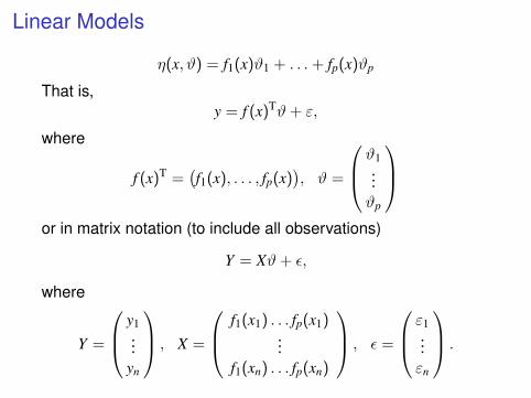
Linear Models
η(x, ϑ) = f1(x)ϑ1 + . . .+ fp(x)ϑp
That is,y = f (x)Tϑ+ ε,
where
f (x)T =(f1(x), . . . , fp(x)
), ϑ =
ϑ1...ϑp
or in matrix notation (to include all observations)
Y = Xϑ+ ε,
where
Y =
y1...
yn
, X =
f1(x1) . . . fp(x1)...
f1(xn) . . . fp(xn)
, ε =
ε1...εn
.
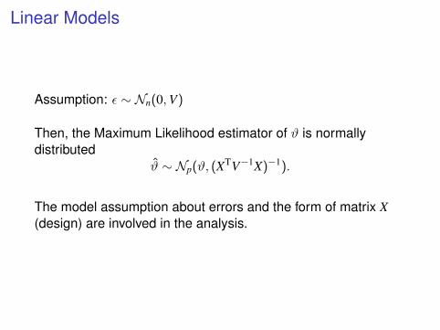
Linear Models
Assumption: ε ∼ Nn(0,V)
Then, the Maximum Likelihood estimator of ϑ is normallydistributed
ϑ̂ ∼ Np(ϑ, (XTV−1X)−1).
The model assumption about errors and the form of matrix X(design) are involved in the analysis.
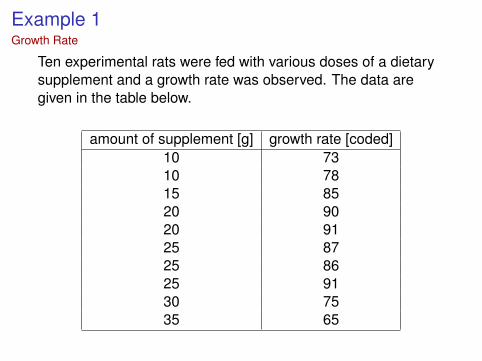
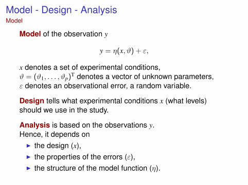
Example 1Growth Rate
Ten experimental rats were fed with various doses of a dietarysupplement and a growth rate was observed. The data aregiven in the table below.
amount of supplement [g] growth rate [coded]10 7310 7815 8520 9020 9125 8725 8625 9130 7535 65
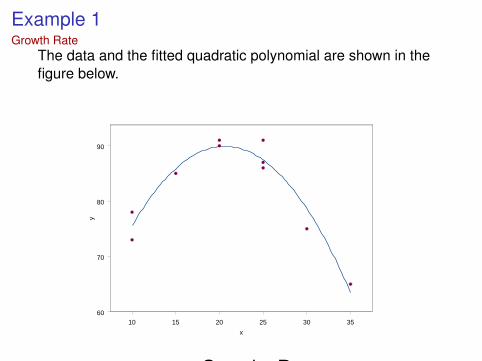
Example 1Growth Rate
The data and the fitted quadratic polynomial are shown in thefigure below.
10 15 20 25 30 35
x
60
70
80
90
y
Figure: Growths Rates

Example 1Growth Rate
A few design questions:
1. Why these particular doses were used?
2. What was known about the plausible response before theexperiment was performed?
3. Could the doses be selected in a better way?
4. How to decide what doses to select and apply?
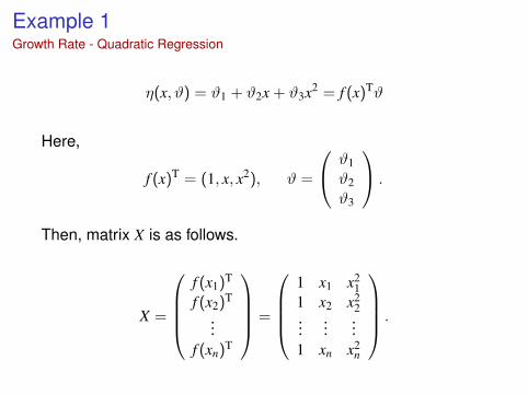
Example 1Growth Rate - Quadratic Regression
η(x, ϑ) = ϑ1 + ϑ2x + ϑ3x2 = f (x)Tϑ
Here,
f (x)T = (1, x, x2), ϑ =
ϑ1ϑ2ϑ3
.
Then, matrix X is as follows.
X =
f (x1)T
f (x2)T
...f (xn)T
=
1 x1 x2
11 x2 x2
2...
......
1 xn x2n
.
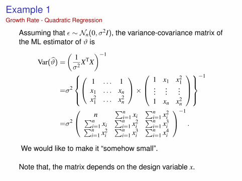
Example 1Growth Rate - Quadratic Regression
Assuming that ε ∼ Nn(0, σ2I), the variance-covariance matrix ofthe ML estimator of ϑ is
Var(ϑ̂) =
(1σ2 XTX
)−1
=σ2
1 . . . 1
x1 . . . xn
x21 . . . x2
n
× 1 x1 x2
1...
......
1 xn x2n
−1
=σ2
n∑n
i=1 xi∑n
i=1 x2i∑n
i=1 xi∑n
i=1 x2i∑n
i=1 x3i∑n
i=1 x2i∑n
i=1 x3i∑n
i=1 x4i
−1
.
We would like to make it “somehow small”.
Note that, the matrix depends on the design variable x.
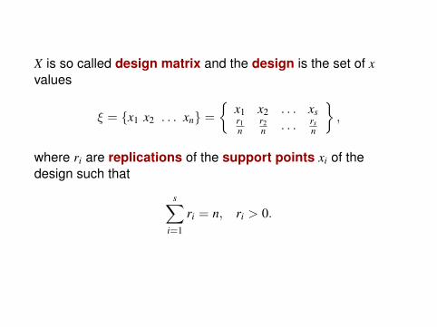
X is so called design matrix and the design is the set of xvalues
ξ = {x1 x2 . . . xn} =
{x1 x2 . . . xsr1n
r2n . . . rs
n
},
where ri are replications of the support points xi of thedesign such that
s∑i=1
ri = n, ri > 0.

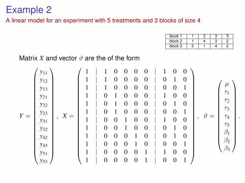
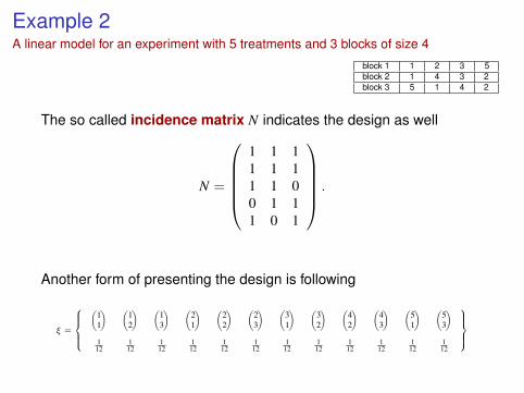
Example 2A linear model for an experiment with 5 treatments and 3 blocks of size 4
Let the allocation of treatments to blocks be following
block 1 1 2 3 5block 2 1 4 3 2block 3 5 1 4 2
The linear model may be written as
yij = µ+ τi + βj + εij,
whereµ denotes the general mean,τi denotes an effect of i-th treatment, i = 1, . . . , 5,βj denotes an effect of j-th block j = 1, 2, 3.
Example 2A linear model for an experiment with 5 treatments and 3 blocks of size 4
block 1 1 2 3 5block 2 1 4 3 2block 3 5 1 4 2
Matrix X and vector ϑ are the of the form
Y =
y11y12y13y21y22y23y31y32y42y43y51y53
, X =
1 | 1 0 0 0 0 | 1 0 01 | 1 0 0 0 0 | 0 1 01 | 1 0 0 0 0 | 0 0 11 | 0 1 0 0 0 | 1 0 01 | 0 1 0 0 0 | 0 1 01 | 0 1 0 0 0 | 0 0 11 | 0 0 1 0 0 | 1 0 01 | 0 0 1 0 0 | 0 1 01 | 0 0 0 1 0 | 0 1 01 | 0 0 0 1 0 | 0 0 11 | 0 0 0 0 1 | 1 0 01 | 0 0 0 0 1 | 0 0 1
, ϑ =
µτ1τ2τ3τ4τ5β1β2β3
.
Example 2A linear model for an experiment with 5 treatments and 3 blocks of size 4
block 1 1 2 3 5block 2 1 4 3 2block 3 5 1 4 2
The so called incidence matrix N indicates the design as well
N =
1 1 11 1 11 1 00 1 11 0 1
.
Another form of presenting the design is following
ξ =
(
11
) (12
) (13
) (21
) (22
) (23
) (31
) (32
) (42
) (43
) (51
) (53
)112
112
112
112
112
112
112
112
112
112
112
112
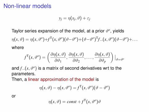
Non-linear models
yj = η(xj, ϑ) + εj
Taylor series expansion of the model, at a prior ϑo, yields
η(x, ϑ) = η(x, ϑo)+f T(x, ϑo)(ϑ−ϑo)+(ϑ−ϑo)Tf ..(x, ϑo)(ϑ−ϑo)+. . .
where
f T(x, ϑo) =
(∂η(x, ϑ)
∂ϑ1,∂η(x, ϑ)
∂ϑ2, . . . ,
∂η(x, ϑ)
∂ϑp
) ∣∣ϑ=ϑo
and f ..(x, ϑo) is a matrix of second derivatives wrt to theparameters.Then, a linear approximation of the model is
η(x, ϑ)− η(x, ϑo) = f T(x, ϑo)(ϑ− ϑo)
orη(x, ϑ) = const + f T(x, ϑo)ϑ
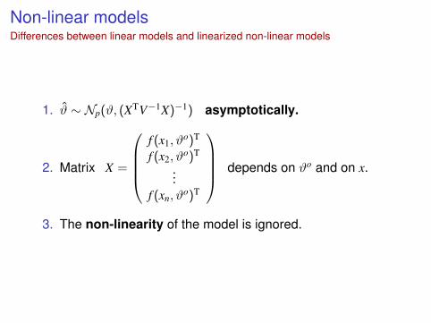
Non-linear modelsDifferences between linear models and linearized non-linear models
1. ϑ̂ ∼ Np(ϑ, (XTV−1X)−1) asymptotically.
2. Matrix X =
f (x1, ϑ
o)T
f (x2, ϑo)T
...f (xn, ϑ
o)T
depends on ϑo and on x.
3. The non-linearity of the model is ignored.
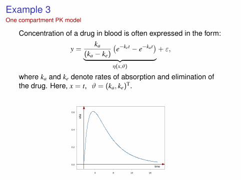
Example 3One compartment PK model
Concentration of a drug in blood is often expressed in the form:
y =ka
(ka − ke)
(e−ket − e−kat)︸ ︷︷ ︸η(x,ϑ)
+ ε,
where ka and ke denote rates of absorption and elimination ofthe drug. Here, x = t, ϑ = (ka, ke)T.
3 8 13 18
time0.0
0.2
0.4
0.6
eta
Example 3One compartment PK model
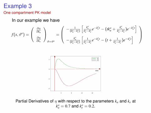
In our example we have
f (x, ϑo) =
∂η∂ka
∂η∂ke
ϑ=ϑo
=
− 1(ko
a−koe )
[ko
eko
a−koee−ko
e t − (tkoa +
koe
koa−ko
e)e−ko
a t]
− koa
(koa−ko
e )
[1
koa−ko
ee−ko
a t − (t + 1ko
a−koe)e−ko
e t]
3 8 13 18
time
-2
-1
0
1f1f2
Partial Derivatives of η with respect to the parameters ka and ke atko
a = 0.7 and koe = 0.2.
Example 3One compartment PK model
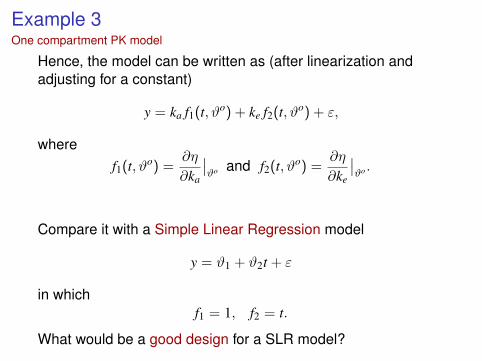
Hence, the model can be written as (after linearization andadjusting for a constant)
y = ka f1(t, ϑo) + ke f2(t, ϑo) + ε,
wheref1(t, ϑo) =
∂η
∂ka
∣∣ϑo and f2(t, ϑo) =
∂η
∂ke
∣∣ϑo .
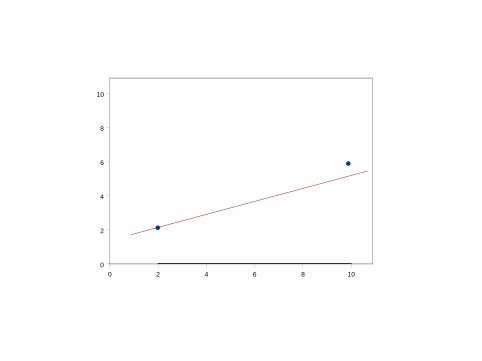
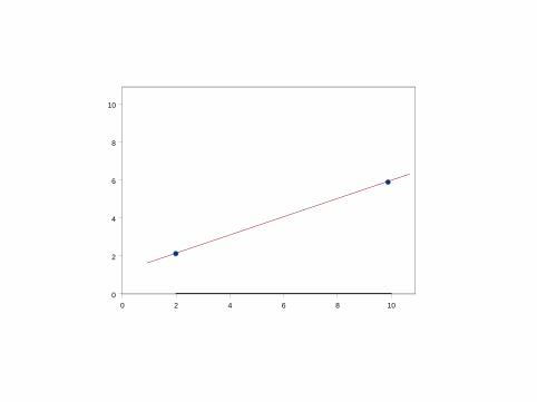
Compare it with a Simple Linear Regression model
y = ϑ1 + ϑ2t + ε
in whichf1 = 1, f2 = t.
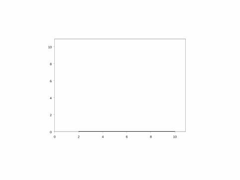
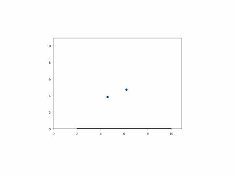
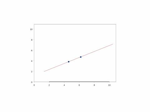
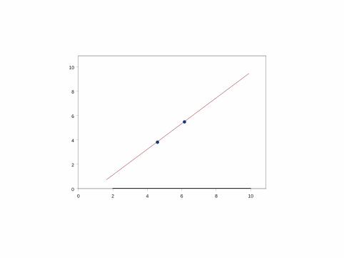
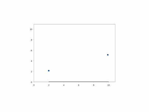
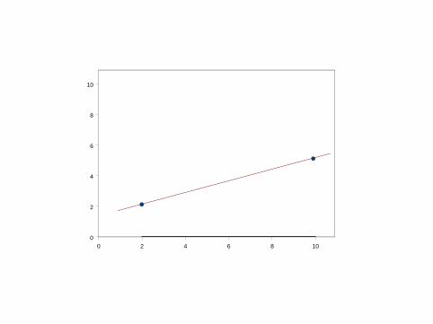
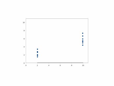
What would be a good design for a SLR model?
0 2 4 6 8 100
2
4
6
8
10
0 2 4 6 8 100
2
4
6
8
10
0 2 4 6 8 100
2
4
6
8
10

0 2 4 6 8 100
2
4
6
8
10
0 2 4 6 8 100
2
4
6
8
10
0 2 4 6 8 100
2
4
6
8
10
0 2 4 6 8 100
2
4
6
8
10
0 2 4 6 8 100
2
4
6
8
10
0 2 4 6 8 100
2
4
6
8
10
0 2 4 6 8 100
2
4
6
8
10
0 2 4 6 8 100
2
4
6
8
10
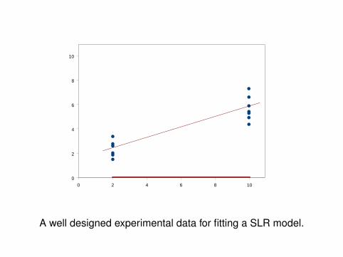
A well designed experimental data for fitting a SLR model.

Big Question
What is the best choice of the design points when the model isnon-linear?
Purpose of an experiment - stats point of view
I estimation of the parameters and their functions (i.g.contrasts) and further testing statistical hypothesis (weknow the family of models),
I model building (no information about the family of models),I model discrimination (there are two or more plausible
families of models),I a combination of estimation and model discrimination,I other.
What is a Design of Experiment?
A plan showing where/when to take observations during anexperiment.
I Classical (combinatorial) designI way of allocating treatments to experimental units,I usually applied for linear models of observations,I treatment structure and unit structure have to be defined
and matched.
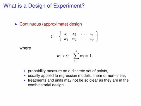
What is a Design of Experiment?
I Continuous (approximate) design
ξ =
{x1 x2 . . . xs
w1 w2 . . . ws
}where
wi > 0,s∑
i=1
wi = 1.
I probability measure on a discrete set of points,I usually applied to regression models, linear or non-linear,I treatments and units may not be so clear as they are in the
combinatorial design.
Optimum Design of Experiments
I A criterion of design optimality has to be specified.
I The criterion will depend on the purpose of theexperiment and on the model.
I When a general form of the model is known, then
I Purpose: estimation of unknown parameters or theirfunctions, or hypothesis testing.
I Design for precision of estimation.
How can we measure the precision of estimation?I via variance and bias of the estimator
Optimum Design of Experiments
I When there are several competing models, thenI Purpose:
I discrimination between the models,I estimation of the parameters and discrimination.
I Design: to optimize for most powerful discrimination and forprecise estimation.
I When there is no information about the model at all,then
I Purpose: to identify the model or some specific values ofinterest,
I Design: to optimize for the specific objective.
Optimum Design of ExperimentsProblems
I In linear models a combinatorial optimum design for aparticular treatment and unit structures may not exist.
I In non-linear models it is possible to find an approximate(continuous) optimum design but it depends on
I prior values of the unknown parameters,
I curvature of the assumed model,
I usually, there are no close form solutions.
I In any case, the optimum design depends on theassumptions regarding the variability and correlation of theobserved response.
Criteria of design optimalityFor parameter estimation
Most of the criteria for parameter estimation were introduced forlinear models and are functions of the Fisher Information Matrix(FIM):
M =
{E(∂L∂ϑi
∂L∂ϑj
)}i,j=1,...,p
,
where L = ln h(ϑ; y) and h(ϑ; y) is the likelihood function for ϑgiven y.
This comes from the (asymptotic) properties of ML estimators:
ϑ̂ ∼approx.
N(ϑ,M−1).
Criteria of design optimalityFor parameter estimation
For a normal linear model of observations
y ∼ N (Xϑ,V),
the likelihood function is
h(ϑ; y) =1
(2π)n/2√|V|
exp{−1
2(y− Xϑ)TV−1(y− Xϑ)
}.
Hence,
L = const − 12
(y− Xϑ)TV−1(y− Xϑ),
∂L∂ϑ
= XTV−1(y− Xϑ),
and
M = E
[∂L∂ϑ
(∂L∂ϑ
)T]
= E[XTV−1(y− Xϑ)(y− Xϑ)TV−1X
]= XTV−1X.
Criteria of design optimalityFor parameter estimation
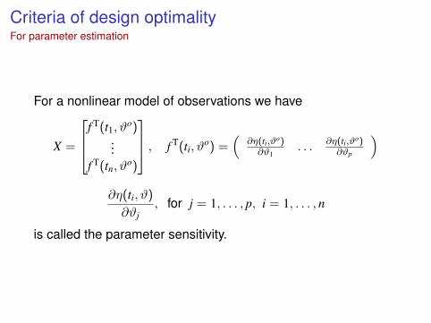
For a nonlinear model of observations we have
X =
f T(t1, ϑo)...
f T(tn, ϑo)
, f T(ti, ϑo) =(
∂η(ti,ϑo)∂ϑ1
. . . ∂η(ti,ϑo)∂ϑp
)
∂η(ti, ϑ)
∂ϑj, for j = 1, . . . , p, i = 1, . . . , n
is called the parameter sensitivity.
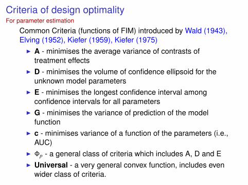
Criteria of design optimalityFor parameter estimation
Common Criteria (functions of FIM) introduced by Wald (1943),Elving (1952), Kiefer (1959), Kiefer (1975)
I A - minimises the average variance of contrasts oftreatment effects
I D - minimises the volume of confidence ellipsoid for theunknown model parameters
I E - minimises the longest confidence interval amongconfidence intervals for all parameters
I G - minimises the variance of prediction of the modelfunction
I c - minimises variance of a function of the parameters (i.e.,AUC)
I Φp - a general class of criteria which includes A, D and EI Universal - a very general convex function, includes even
wider class of criteria.