DESCRIPTION OF THE SUBROUTINES USED TO COMPUTE GROUND …
106
6S User Guide Version 3, November 2006 138 DESCRIPTION OF THE SUBROUTINES USED TO COMPUTE GROUND BRDF
Transcript of DESCRIPTION OF THE SUBROUTINES USED TO COMPUTE GROUND …
6S User Guide Version 3, November 2006
138
DESCRIPTION OF THE SUBROUTINES USED
TO COMPUTE GROUND BRDF
6S User Guide Version 3, November 2006
139
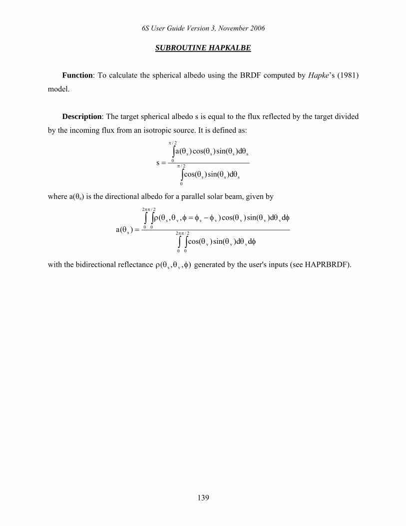
SUBROUTINE HAPKALBE
Function: To calculate the spherical albedo using the BRDF computed by Hapke’s (1981)
model.
Description: The target spherical albedo s is equal to the flux reflected by the target divided
by the incoming flux from an isotropic source. It is defined as:
∫
∫π
π
θθθ
θθθθ= 2/
0sss
2/
0ssss
d)sin()cos(
d)sin()cos()(as
where a(θs) is the directional albedo for a parallel solar beam, given by
∫ ∫
∫ ∫ππ
ππ
φθθθ
φθθθφ−φ=φθθρ=θ 2
0
2/
0vvv
2
0
2/
0vvvvsvs
s
dd)sin()cos(
dd)sin()cos(),,()(a
with the bidirectional reflectance ),,( vs φθθρ generated by the user's inputs (see HAPRBRDF).
6S User Guide Version 3, November 2006
140
SUBROUTINE IAPIALBE
Function: Same as HAPKALBE but for a BRDF from the subroutine IAPIBRDF.
SUBROUTINE MINNALBE
Function: Same as HAPKALBE but for a BRDF from the subroutine MINNBRDF.
SUBROUTINE OCEALBE (and GLITALBE)
Function: Same as HAPKALBE but for a BRDF from the subroutine OCEABRDF.
SUBROUTINE RAHMALBE
Function: Same as HAPKALBE but for a BRDF from the subroutine RAHMBRDF.
SUBROUTINE ROUJALBE
Function: Same as HAPKALBE but for a BRDF from the subroutine ROUJBRDF.
SUBROUTINE VERSALBE
Function: Same as HAPKALBE but for a BRDF from the subroutine VERSBRDF.
SUBROUTINE WALTALBE
Function: Same as HAPKALBE but for a BRDF from the subroutine WALTBRDF.
6S User Guide Version 3, November 2006
141
SUBROUTINE BRDFGRID
Function: To generate a BRDF following the user's inputs.
Description: The user enters the value of ρ for the Sun at a given sun zenith angle θs for the
view zenith angle θv ranging from 0° to 80° by steps of 10° and equal to 85°, and for the view
azimuth angle vφ ranging from 0° to 360° by steps of 30°. The user does the same for the Sun
which would be at θv. In addition, the spherical albedo of the surface and observed reflectance in
the selected geometry ),,,( vsvs φφθθρ need to be specified.
Parameters:
1. for θs the user has to enter ),( vv φθρ :
ρ(0°,0°), ρ(10°,0°), ... ρ(80°,0°), ρ(85°,0°)
ρ(0°,30°), ρ(10°,30°), ... ρ(80°,30°), ρ(85°,30°)
...
ρ(0°,360°), ρ(10°,360°), ... ρ(80°,360°), ρ(85°,360°)
2. for θs=θv the user has to enter ),( vv φθρ :
ρ(0°,0°), ρ(10°,0°), ... ρ(80°,0°), ρ(85°,0°)
ρ(0°,30°), ρ(10°,30°), ... ρ(80°,30°), ρ(85°,30°)
...
ρ(0°,360°), ρ(10°,360°), ... ρ(80°,360°), ρ(85°,360°)
3. the spherical albedo of the surface
4. the observed reflectance in the selected geometry ),,,( vsvs φφθθρ
6S User Guide Version 3, November 2006
142
SUBROUTINE HAPKBRDF
Function: To generate a BRDF following Hapke's (1981) model.
Description (from Pinty & Verstraete, 1991): From the fundamental principles of radiative
transfer theory, Hapke (1981) derived an analytical equation for the bidirectional reflectance
function of a medium composed of dimensionless particles. The singly scattered radiance is
derived exactly, whereas the multiply scattered radiance is evaluated from a two-stream
approximation, assuming that the scatterers making up the surface are isotropic. The
bidirectional reflectance ρ of a surface illuminated by the sun from a direction ),( ss φθ , observed
from a direction ),( vv φθ , and normalized with respect to the reflectance of a perfectly reflecting
Lambertian surface under the same condition is given by
[ ] 1)(H)(H)g(P)g(B114
),,,( vsvs
vvss −µµ++µ+µ
ω=φθφθρ ,
where
ω is the average single scattering albedo of medium particles,
)cos( ss θ=µ and )cos( vv θ=µ ,
g is the phase angle between the incoming and outgoing rays, defined as
)cos()sin()sin()cos()cos()gcos( vsvsvs φ−φθθ+θθ= ,
B(g) is a backscattering function that accounts for the hot spot effect:
[ ])2/gtan()h/1(1)0(P)0(S)g(B
+ω= ,
with the amplitude and width of the hot spot S(0) and h,
P(g) is the average phase function of medium particles, computed here by the Heyney and
Greenstein's function:
)gcos(211)g(P 2
2
Θ+Θ+Θ−
=
with the asymmetry factor Θ ranging from -1 (backward scattering) to +1 (forward scattering),
and H(µ) is a function to account for multiple scattering:
µω−+µ+
=µ 2/1)1(2121)(H .
6S User Guide Version 3, November 2006
143
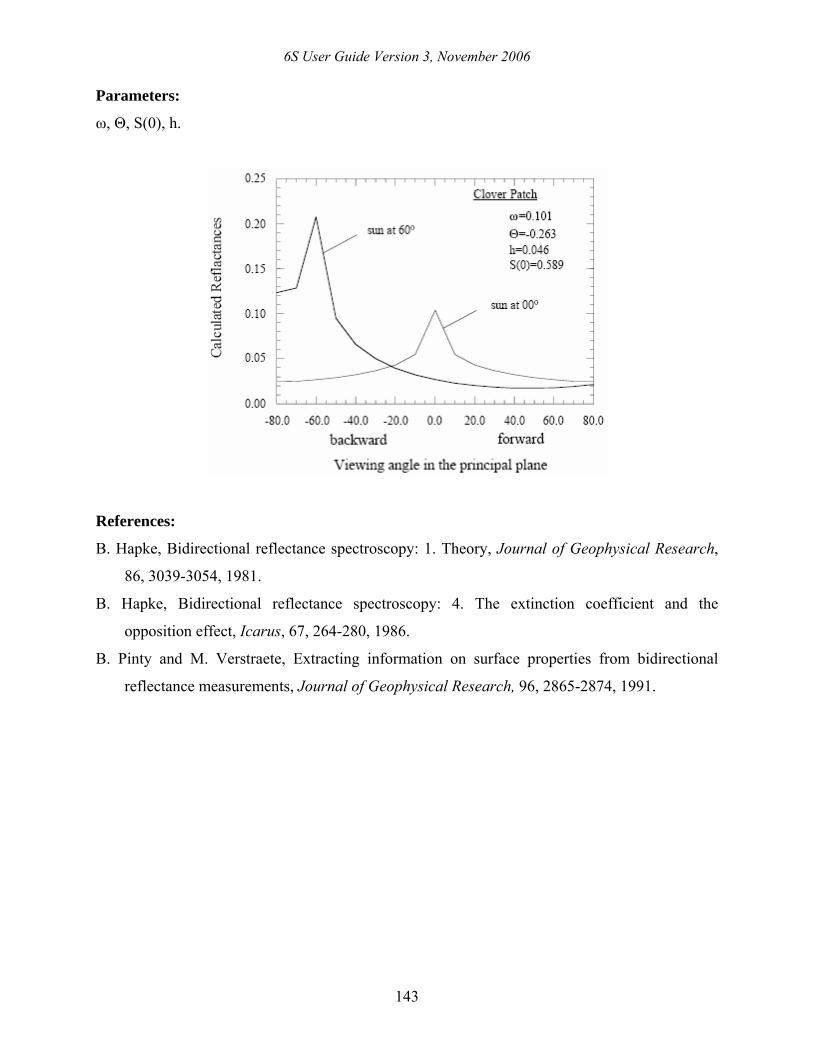
Parameters:
ω, Θ, S(0), h.
References:
B. Hapke, Bidirectional reflectance spectroscopy: 1. Theory, Journal of Geophysical Research,
86, 3039-3054, 1981.
B. Hapke, Bidirectional reflectance spectroscopy: 4. The extinction coefficient and the
opposition effect, Icarus, 67, 264-280, 1986.
B. Pinty and M. Verstraete, Extracting information on surface properties from bidirectional
reflectance measurements, Journal of Geophysical Research, 96, 2865-2874, 1991.
6S User Guide Version 3, November 2006
144
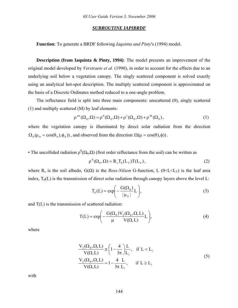
SUBROUTINE IAPIBRDF
Function: To generate a BRDF following Iaquinta and Pinty's (1994) model.
Description (from Iaquinta & Pinty, 1994): The model presents an improvement of the
original model developed by Verstraete et al. (1990), in order to account for the effects due to an
underlying soil below a vegetation canopy. The singly scattered component is solved exactly
using an analytical hot-spot description. The multiply scattered component is approximated on
the basis of a Discrete Ordinates method reduced to a one-angle problem.
The reflectance field is split into three main components: unscattered (0), singly scattered
(1) and multiply scattered (M) by leaf elements:
)(),(),(),( 0M
01
00
0tot Ωρ+ΩΩρ+ΩΩρ=ΩΩρ , (1)
where the vegetation canopy is illuminated by direct solar radiation from the direction
))),cos(( 0000 φθ=µΩ , and observed from the direction ))),cos(( φθ=µΩ .
• The uncollided radiation ρ0(Ω0,Ω) (first order reflectance from the soil) can be written as
)L(T)L(TR),( TT0s00 =ΩΩρ , (2)
where Rs is the soil albedo, G(Ω) is the Ross-Nilson G-function, L (0<L<LT) is the leaf area
index, T0(L) is the transmission of direct solar radiation through canopy layers above the level L:
⎟⎟⎠
⎞⎜⎜⎝
⎛µΩ
−= L||)(G
exp)L(T0
00 , (3)
and T(L) is the transmission of scattered radiation:
⎟⎟⎠
⎞⎜⎜⎝
⎛Ωµ
ΩΩΩ−= L
)L,(V)L,,(V)(G
exp)L(T 020 , (4)
where
ii
02
ii
02
LLif ,LL
341
)L,(V)L,,(V
LLif,LL
341
)L,(V)L,,(V
≥π
−=ΩΩΩ
<⎟⎠⎞
⎜⎝⎛
π−≅
ΩΩΩ
(5)
with
6S User Guide Version 3, November 2006
145
)cos()tan()tan(2)(tan)(tan
r2L00
20
2iφ−φθθ−θ+θ
Λ= . (6)
Here Λ denotes the leaf area density [m2m-3] and r [m] is the radius of sun-flecks on an
illuminated leaf.
• The single scattering by canopy elements ρ1(Ω0,Ω) is given by
∫µµΩ→ΩΓ
=ΩΩρTL
00
0
00
1 dL)L(T)L(T||
)(),( , (7)
where
Γ(Ω0→Ω) is the area scattering phase function (bi-Lambertian).
• Using a canopy transport equation reduced to a one-angle problem and assuming isotropic
scattering, the multiply scattered radiation exiting at the top of canopy is given by
'd')',0(I||
1)(1
0
M
00
M µµµµ
=Ωρ ∫ , (8)
where IM is the intensity of photons which have been scattered twice or more times in the
canopy.
The G(Ω) function is the leaf area projected to the direction Ω by a unit leaf area:
∫+π
ΩΩ⋅ΩΩπ
=Ω2
LLLL d||)(g21)(G , (9)
where gL(ΩL) is the probability density of the distribution of leaf normals with respect to the
upward hemisphere (its computation depends on the input parameter ild).
The area scattering phase function Γ(Ω0→Ω) is given by
LL2
LLL d),'(f')(g21)'(1
ΩΩΩ→ΩΩ⋅ΩΩπ
=Ω→ΩΓπ ∫
+π
, (10)
where ),'(f LΩΩ→Ω is the leaf scattering distribution function. Here it is assumed that the
leaves follow a bi-Lambertian scattering model, and ),'(f LΩΩ→Ω is defined as
⎪⎩
⎪⎨
⎧
>Ω⋅ΩΩ⋅ΩπΩ⋅Ω
<Ω⋅ΩΩ⋅ΩπΩ⋅Ω
=ΩΩ→Ω0)')((if ,||t
0)')((if ,||r
),'(fLL
LL
LLLL
L , (11)
6S User Guide Version 3, November 2006
146
with rL and tL are the leaf reflection and transmission coefficients.
Parameters:
1 - ild, ihs
2 - LT, 2rΛ
3 - rL, tL, RS
where ild is the leaf angle distribution (1=planophile, 2=erectophile, 3=plagiophile,
4=extremophile, and 5=uniform), ihs is a hot spot descriptor (0=no hot-spot, 1=hot spot), LT the
leaf area index in [1.0, 15.0], 2rΛ is a hot-spot parameter in [0.0 (no hot-spot), 2.0], rL is the leaf
reflection coefficient in [0.0, 0.99], tL is the leaf transmission coefficient in [0.0, 0.99], and RS is
the soil albedo in [0.0, 0.99].
References:
J. Iaquinta, and B. Pinty, Adaptation of a bidirectional reflectance model including the hot-spot
to an optically thin canopy, Proceedings of the VI International Colloquium: Physical
measurements and signatures in remote sensing, Val d'Isère, France, 683-690, 1994.
M. Verstraete, B. Pinty, and R.E. Dickinson, A physical model of the bidirectional reflectance of
vegetation canopies: 1. Theory, Journal of Geophysical Research, 95, 11755-11765, 1990.
6S User Guide Version 3, November 2006
147
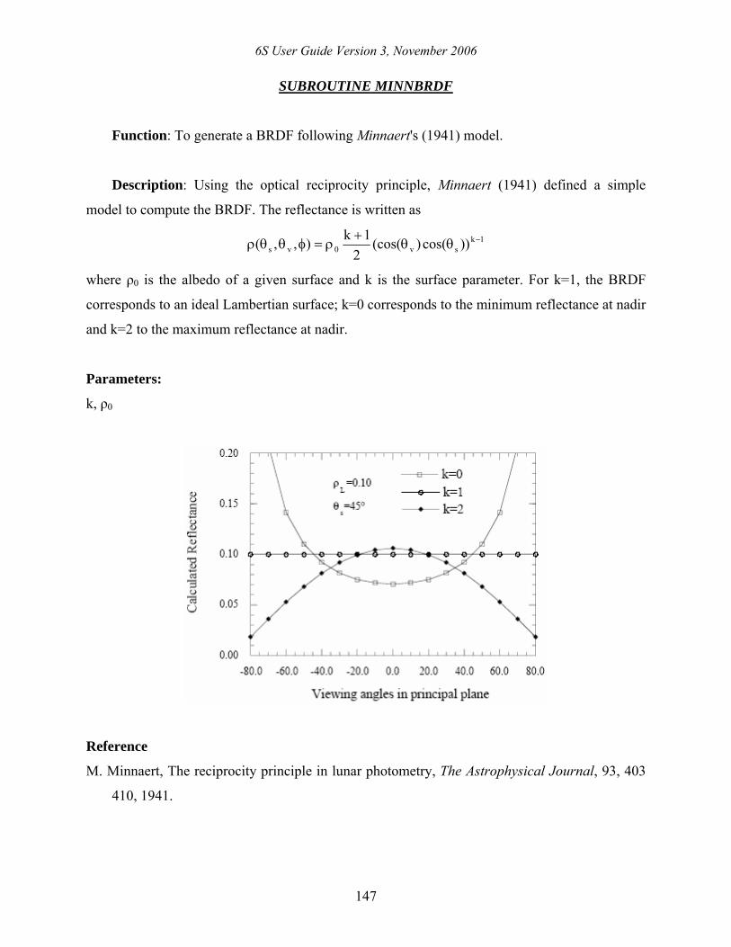
SUBROUTINE MINNBRDF
Function: To generate a BRDF following Minnaert's (1941) model.
Description: Using the optical reciprocity principle, Minnaert (1941) defined a simple
model to compute the BRDF. The reflectance is written as
1ksv0vs ))cos()(cos(
21k),,( −θθ
+ρ=φθθρ
where ρ0 is the albedo of a given surface and k is the surface parameter. For k=1, the BRDF
corresponds to an ideal Lambertian surface; k=0 corresponds to the minimum reflectance at nadir
and k=2 to the maximum reflectance at nadir.
Parameters:
k, ρ0
Reference
M. Minnaert, The reciprocity principle in lunar photometry, The Astrophysical Journal, 93, 403
410, 1941.
6S User Guide Version 3, November 2006
148
SUBROUTINE OCEABRDF (and OCEATOOLS)
Function: To compute the BRDF of an ocean surface by taking into account the influence of
whitecaps, sun glint and pigment concentration.
Description: In the solar spectral range, the reflectance of an ocean surface ρos(λ) can be
assumed for a given set of geometrical condition θs, θv and φ (=ϕs-ϕv) as the sum of three
components dependent on the wavelength λ (Koepke, 1984):
),,,()(1),,,(W1)(),,,( vsswwcvsglwcvsos λφθθρ⋅λρ−+λφθθρ⋅−+λρ=λφθθρ ,
where
• ρwc(λ) is the reflectance due to whitecaps,
• ρgl(λ) is the specular reflectance at the ocean surface,
• ρsw(λ) is the scattered reflectance emerging from sea water, and
• W is the relative area covered with whitecaps, which can be expressed from the wind speed ws
(Monahan & O'Muircheartaigh, 1980) as W=2.9510-6ws3.52 for water temperatures greater than
14°C.
1 - Reflectance of whitecaps ρwc(λ)
According to Koepke (1984), "the optical influence of whitecaps is given by the product of
the area of each individual whitecap W and its corresponding reflectance ρf(λ). However, the
area of an individual whitecap increases with its age, while its reflectance decreases. Since
whitecaps of different ages are taken into consideration in the W values, the combination of W
with ρf(λ) gives ρwc(λ) values that are too high". Thus Koepke defines, instead of ρf(λ), an
effective reflectance of ocean foam patches ρef(λ) and calculates ρwc(λ) as
)(fW)(W)( fefefwc λρ⋅⋅=λρ⋅=λρ ,
where fef is the efficiency factor slightly dependent on the wind speed but independent of the
wavelength (fef = 0.4± 0.2).
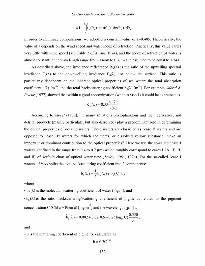
Figure 1 shows the reflectance of whitecaps as a function of the wind speed in the visible
spectral range; in this range the effective reflectance ρef(λ) is a constant value (22 ± 11)%.
6S User Guide Version 3, November 2006
149
2 - Reflectance of the sun glint ρgl(λ) (SUBROUTINE SUNGLINT)
Cox & Munk (1954, 1955) made measurements of the sun glitter from aerial photographs.
They defined a many-faceted model surface whose wave-slopes vary according to isotropic and
anisotropic Gaussian distributions with respect to the surface wind.
Lets consider the system of coordinates (P;X,Y,Z) where P is the observed point, Z is the
altitude, PY is pointed at the sun direction and PX at the direction perpendicular to the sun plane.
In this system, the surface slope is defined by its two components Zx and Zy,
)tan()cos(YZZand)tan()sin(
XZZ yx βα=
∂∂
=βα=∂∂
= ,
where α is the azimuth of the ascent (clockwise from the sun) and β is the tilt. Using spherical
trigonometry, Zx and Zy can be related to the incident and reflected directions ( s2/ θ≥π and
0v ≥θ ) as
)cos()cos()cos()sin()sin(
Zand)cos()cos(
)sin()sin(Z
vs
vsvsy
vs
vsvx θ+θ
ϕ−ϕθ+θ=
θ+θϕ−ϕθ−
= .
For the case of an anisotropic distribution of slope components (dependent on the wind
direction), lets consider new principal axes (P;X',Y',Z'=Z) defined by a rotation of χ from the sun
(P;X,Y,Z) system with PY' parallel to the wind direction (related clockwise from the North by
φw, then χ = φs - φw) The slope components are now expressed as
yXyyXX Z)(conZ)sin('ZandZ)sin(Z)cos('Z ⋅χ+⋅χ−=⋅χ+⋅χ= ,
and the slope distribution is expressed by a Gram-Charlier series as
⎭⎬⎫+η−η+−η−ξ++ξ−ξ+
⎩⎨⎧ η−η−−ξ−
η+ξ−
σπσ=
)36(C241)1)(1(C
41)36(C
241
)(C61)1(C
211)
2exp(
''21)'Z,'Z(P
2404
2222
2440
303
221
22
yxyx
,
where
ξ=Zx'/σx' and η=Zy'/σy',
σx' and σy' are the rms values of Zx' and Zy', the skewness coefficients C21 and C03, and the
peakedness coefficients C40, C22 and C04 are defined by Cox & Munk (1954, 1955) for a clean
(uncontaminated) surface as
6S User Guide Version 3, November 2006
150
,004.0ws00316.0)'(,002.0ws00192.0003.0)'( 2y
2x ±=σ±+=σ
C21 = 0.01 − 0.0086ws ± 0.03 , C03 = 0.04 − 0.033ws ± 0.12,
C40 = 0. 40 ± 0.23 , C22 = 0.12 ± 0.06, and C04 = 0.23 ± 0. 41.
Thus, the directional reflectance is written as
)(cos)cos()cos(4),,,,n(R)'Z,'Z(P
),,,( 4vs
vsvsyxvsvsgl βθθ
ϕϕθθπ=ϕϕθθρ ,
where ),,,,n(R vsvs ϕϕθθ is Fresnel's reflection coefficient (n is the complex refractive index of
sea water), defined below.
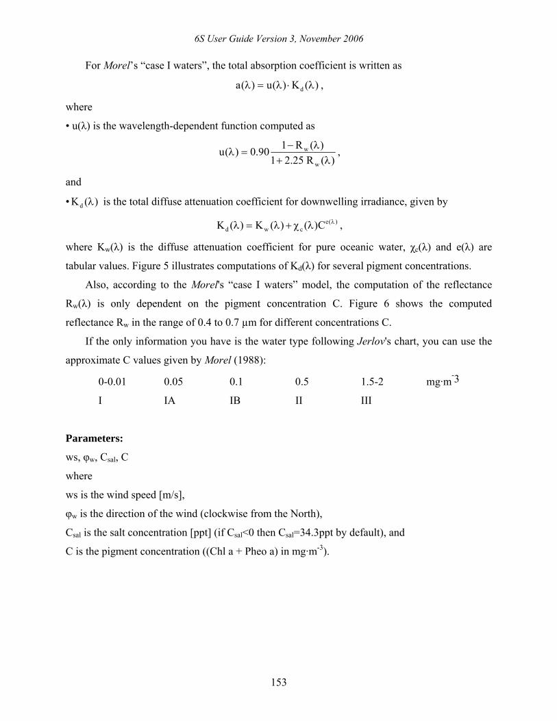
Figure 2 shows computations of ρgl for the wind speed of 5 and 15m/s, χ equal to 0, 90, 180,
and 270°, solar zenith angle of 30°, and wavelength of 0.550µm.
3 - Fresnel's reflection coefficient (SUBROUTINE FRESNEL and INDWAT)
The reflection coefficient ),,,,n(R vsvs ϕϕθθ is computed (Born & Wolf, 1975) involving
the absorption of water ( n = n − ini ) as
[ ] [ ][ ] [ ]2iir
2i
2i
2r
2iir
2i
2i
2r
vsvsv)cos(nn2u)cos()nn(
v)cos(nn2u)cos()nn(21),,,,n(R
−θ++θ−
+θ+−θ−=ϕϕθθ
with
[ ] 2i
2r
2i
22i
2ri
22i
2r
2 nn4)(sinnn|)(sinnn|21u +θ−−+θ−−= ,
[ ] 2i
2r
2i
22i
2ri
22i
2r
2 nn4)(sinnn|)(sinnn|21v +θ−−+θ−−−= ,
[ ])sin()sin()sin()cos()cos(121)cos( vsvsvsi ϕ−ϕθθ+θθ+=θ , and
[ ])sin()sin()sin()cos()cos(121)sin( vsvsvsi ϕ−ϕθθ+θθ−=θ .
In 6S, the complex index of refraction of sea water (we assume that the outside medium is
vacuum) is deduced from the complex index of refraction of pure water, specified by Hale &
Querry (1973). By default, we assume a typical sea water (salinity=34.3ppt, chlorinity=19ppt) as
reported by Sverdrup (1942, p.173). McLellan (1965, p.129) reported that the index of refraction
increased as a function of chlorinity. For the chlorinity of 19.0 ppt, the increase was found to
6S User Guide Version 3, November 2006
151
have a value of +0.006 and be linear with the salt concentration Csal (see also Friedman, 1969).
For the extinction coefficient, Friedman (1969) reported that no correction was required between
1.5 and 9 µm.
Thus, in 6S we apply the correction δnr of +0.006 on the index of refraction of pure water
and no correction δni for the extinction coefficient. The user is able to enter his/her own salt
concentration. In this case, a linear interpolation is assumed to correct the index of refraction of
pure water, so that δnr = 0 for Csal = 0ppt and δnr =+0.006 for Csal =34.3ppt.
4 - Reflectance emerging from sea water ρsw(λ) (SUBROUTINE MORCASIWAT for Rw)
The reflectance emerging from sea water (also called the remote sensing reflectance of sea
water) ),,,( vssw λφθθρ is the reflectance observed just above the sea surface (level 0+).This
reflectance can be related to the reflectance Rw, which is the ratio of upwelling to downwelling
radiance just below the sea surface (level 0-) If we assume that the ocean is a Lambertian
reflector, ),,,( vssw λφθθρ can be expressed as
)(Ra1)(t)(t)(R
n1),,,(
w
vusdw2vssw λ⋅−
θ⋅θ⋅λ=λφθθρ ,
where • td is the transmittance for downwelling radiance, calculated using the Fresnel reflectance
coefficient ),,(R dswa φθθ− for the air-water interface as
φ⋅θ⋅θ⋅θ⋅φθθ−=θ ∫ ∫π π
− dd)sin()cos(),,(R1)(t ad
ad
ad
2
0
2/
0
adswasd .
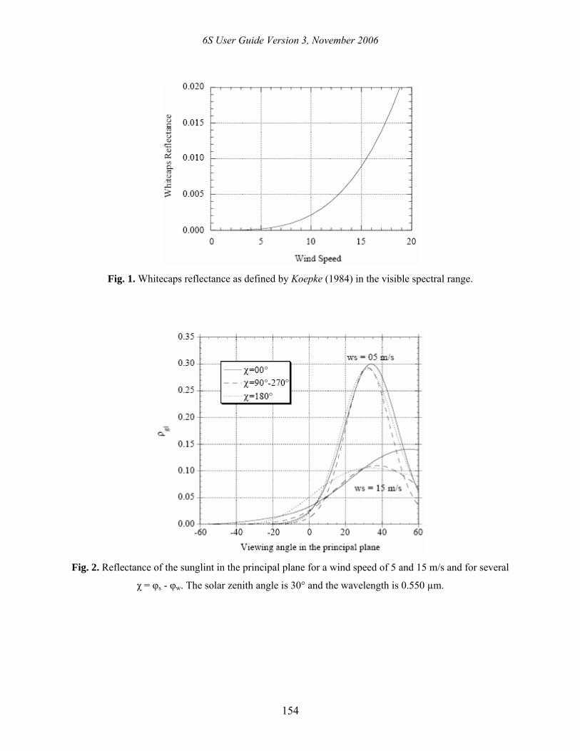
The angle θd represents (see Fig. 3) the zenith angle of a reflected solar beam according to the
wave-slopes distribution (Cox & Munk's model, see below).
• tu is the transmittance for upwelling radiance, calculated using the Fresnel reflectance
coefficient ),,(R uswa φθθ− for the water-air interface as
φ⋅θ⋅θ⋅θ⋅φθθ−=θ ∫ ∫π π
− dd)sin()cos(),,(R1)(t wu
wu
wu
2
0
2/
0
wuvawvu .
The angle wuθ represents (see Fig. 3) the zenith angle of an upwelling beam in the water,
according to Fresnel & Snell's law (nairsin(θair) = nseasin(θsea)) and the wave-slopes distribution.
• a is defined by
6S User Guide Version 3, November 2006
152
vvv
2/
0vu d)sin()cos()(t1a θ⋅θ⋅θ⋅θ−= ∫
π
.
In order to minimize computations, we adopted a constant value of a=0.485. Theoretically, the
value of a depends on the wind speed and water index of refraction. Practically, this value varies
very little with wind speed (see Table 2 of Austin, 1974), and the index of refraction of water is
almost constant in the wavelength range from 0.4µm to 0.7µm and assumed to be equal to 1.341.
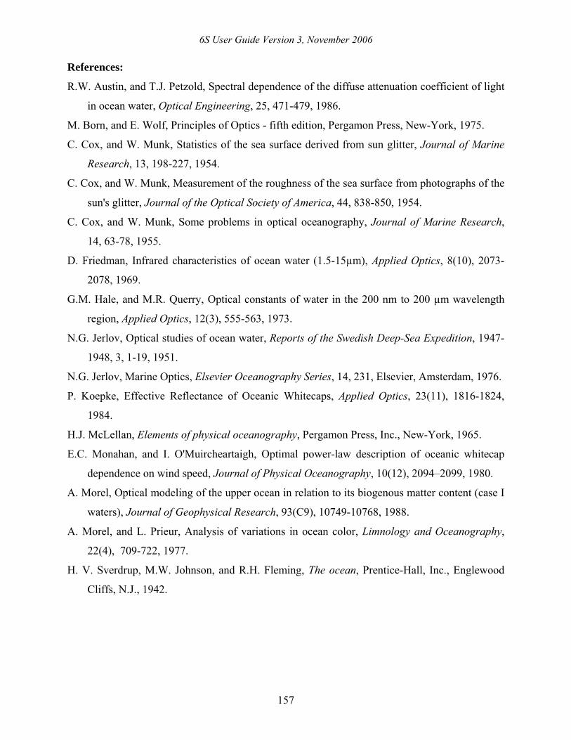
As described above, the irradiance reflectance Rw(λ) is the ratio of the upwelling spectral
irradiance Eu(λ) to the downwelling irradiance Ed(λ) just below the surface. This ratio is
particularly dependent on the inherent optical properties of sea water: the total absorption
coefficient a(λ) [m-1] and the total backscattering coefficient bb(λ) [m-1]. For example, Morel &
Prieur (1977) showed that within a good approximation (when a(λ)<<1) it could be expressed as
)(a)(b33.0)(R b
w λλ
=λ .
According to Morel (1988), "in many situations phytoplanktons and their derivative, and
detrital products (mainly particulate, but also dissolved) play a predominant role in determining
the optical properties of oceanic waters. These waters are classified as "case I" waters and are
opposed to "case II" waters for which sediments, or dissolved yellow substance, make an
important or dominant contribution to the optical properties". Here we use the so-called "case I
waters" (defined in the range from 0.4 to 0.7 µm) which roughly correspond to cases I, IA, IB, II,
and III of Jerlov's chart of optical water type (Jerlov, 1951, 1976). For the so-called "case I
waters", Morel splits the total backscattering coefficient into 2 components:
b)(b~)(b21)(b bwb ⋅λ+λ=λ ,
where
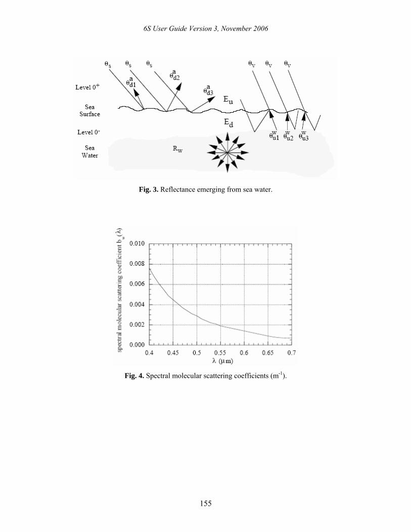
• bw(λ) is the molecular scattering coefficient of water (Fig. 4), and
• )(b~b λ is the ratio backscattering/scattering coefficient of pigments, related to the pigment
concentration C (Chl a + Pheo a) [mg·m-3
] and the wavelength [µm] as
λ−+=λ
550.0)Clog25.05.0(02.0002.0)(b~ 10b ,
and
• b is the scattering coefficient of pigments, calculated as 62.0C3.0b = .
6S User Guide Version 3, November 2006
153
For Morel’s “case I waters”, the total absorption coefficient is written as
)(K)(u)(a d λ⋅λ=λ ,
where
• u(λ) is the wavelength-dependent function computed as
)(R25.21)(R190.0)(u
w
w
λ+λ−
=λ ,
and
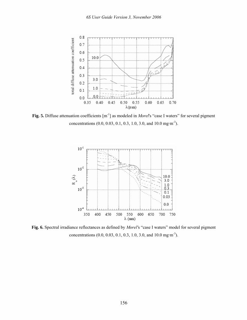
• )(Kd λ is the total diffuse attenuation coefficient for downwelling irradiance, given by
)(ecwd C)()(K)(K λλχ+λ=λ ,
where Kw(λ) is the diffuse attenuation coefficient for pure oceanic water, χc(λ) and e(λ) are
tabular values. Figure 5 illustrates computations of Kd(λ) for several pigment concentrations.
Also, according to the Morel's “case I waters” model, the computation of the reflectance
Rw(λ) is only dependent on the pigment concentration C. Figure 6 shows the computed
reflectance Rw in the range of 0.4 to 0.7 µm for different concentrations C.
If the only information you have is the water type following Jerlov's chart, you can use the
approximate C values given by Morel (1988):
0-0.01 0.05 0.1 0.5 1.5-2 mg·m-3
I IA IB II III
Parameters:
ws, φw, Csal, C
where
ws is the wind speed [m/s],
φw is the direction of the wind (clockwise from the North),
Csal is the salt concentration [ppt] (if Csal<0 then Csal=34.3ppt by default), and
C is the pigment concentration ((Chl a + Pheo a) in mg·m-3).
6S User Guide Version 3, November 2006
154
Fig. 1. Whitecaps reflectance as defined by Koepke (1984) in the visible spectral range.
Fig. 2. Reflectance of the sunglint in the principal plane for a wind speed of 5 and 15 m/s and for several
χ = φs - φw. The solar zenith angle is 30° and the wavelength is 0.550 µm.
6S User Guide Version 3, November 2006
155
Fig. 3. Reflectance emerging from sea water.
Fig. 4. Spectral molecular scattering coefficients (m-1).
6S User Guide Version 3, November 2006
156
Fig. 5. Diffuse attenuation coefficients [m-1] as modeled in Morel's “case I waters” for several pigment
concentrations (0.0, 0.03, 0.1, 0.3, 1.0, 3.0, and 10.0 mg·m-3).
Fig. 6. Spectral irradiance reflectances as defined by Morel's “case I waters” model for several pigment
concentrations (0.0, 0.03, 0.1, 0.3, 1.0, 3.0, and 10.0 mg·m-3).
6S User Guide Version 3, November 2006
157
References:
R.W. Austin, and T.J. Petzold, Spectral dependence of the diffuse attenuation coefficient of light
in ocean water, Optical Engineering, 25, 471-479, 1986.
M. Born, and E. Wolf, Principles of Optics - fifth edition, Pergamon Press, New-York, 1975.
C. Cox, and W. Munk, Statistics of the sea surface derived from sun glitter, Journal of Marine
Research, 13, 198-227, 1954.
C. Cox, and W. Munk, Measurement of the roughness of the sea surface from photographs of the
sun's glitter, Journal of the Optical Society of America, 44, 838-850, 1954.
C. Cox, and W. Munk, Some problems in optical oceanography, Journal of Marine Research,
14, 63-78, 1955.
D. Friedman, Infrared characteristics of ocean water (1.5-15µm), Applied Optics, 8(10), 2073-
2078, 1969.
G.M. Hale, and M.R. Querry, Optical constants of water in the 200 nm to 200 µm wavelength
region, Applied Optics, 12(3), 555-563, 1973.
N.G. Jerlov, Optical studies of ocean water, Reports of the Swedish Deep-Sea Expedition, 1947-
1948, 3, 1-19, 1951.
N.G. Jerlov, Marine Optics, Elsevier Oceanography Series, 14, 231, Elsevier, Amsterdam, 1976.
P. Koepke, Effective Reflectance of Oceanic Whitecaps, Applied Optics, 23(11), 1816-1824,
1984.
H.J. McLellan, Elements of physical oceanography, Pergamon Press, Inc., New-York, 1965.
E.C. Monahan, and I. O'Muircheartaigh, Optimal power-law description of oceanic whitecap
dependence on wind speed, Journal of Physical Oceanography, 10(12), 2094–2099, 1980.
A. Morel, Optical modeling of the upper ocean in relation to its biogenous matter content (case I
waters), Journal of Geophysical Research, 93(C9), 10749-10768, 1988.
A. Morel, and L. Prieur, Analysis of variations in ocean color, Limnology and Oceanography,
22(4), 709-722, 1977.
H. V. Sverdrup, M.W. Johnson, and R.H. Fleming, The ocean, Prentice-Hall, Inc., Englewood
Cliffs, N.J., 1942.
6S User Guide Version 3, November 2006
158
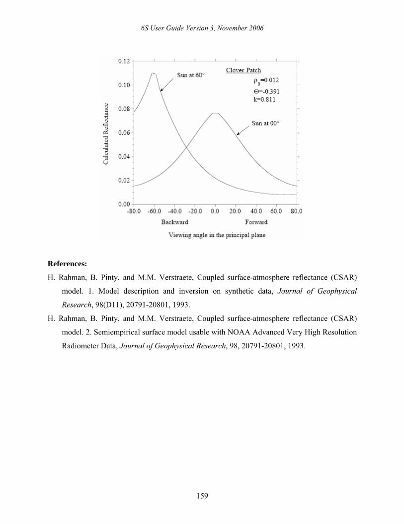
SUBROUTINE RAHMBRDF
Function: To generate a BRDF following Rahman et al.'s model.
Description (from Raman et al., 1993): It’s a semiempirical model for arbitrary natural
surfaces in visible and near-infrared spectra on the basis of 3 parameters. The reflectance ρs of a
surface illuminated from a direction ),( ss φθ and observed from a direction ),( vv φθ is
calculated as
)]G(R1)[g(F)cos(cos
coscos),,,( k1
vs
v1k
s1k
0vvsss +θ+θ
θθρ=φθφθρ −
−−
,
where
ρ0 is the arbitrary parameter characterizing the intensity of the reflectance of the surface cover,
k is the structural parameter indicating the level of anisotropy of the surface,
F(g) is the modified Henyey & Greenstein’s function defined as
5.12
2
)]gcos(21[1)g(F
−πΘ−Θ+Θ−
= ,
with the phase angle g given by
)cos(sinsincoscosgcos vsvsvs φ−φθθ+θθ=
and the asymmetry factor Θ controlling the relative amount of forward ( 10 +≤Θ≤ ) and
backward ( 10 −≤Θ≤ ) scattering,
and R(g) is the function accounting for the hot spot effect, defined as
G11
)G(R 0
+ρ−
= ,
with the geometric factor G given by 2/1
vsvsv2
s2 )]cos(tantan2tan[tanG φ−φθθ−θ+θ= .
Parameters:
ρ0, Θ, k
6S User Guide Version 3, November 2006
159
References:
H. Rahman, B. Pinty, and M.M. Verstraete, Coupled surface-atmosphere reflectance (CSAR)
model. 1. Model description and inversion on synthetic data, Journal of Geophysical
Research, 98(D11), 20791-20801, 1993.
H. Rahman, B. Pinty, and M.M. Verstraete, Coupled surface-atmosphere reflectance (CSAR)
model. 2. Semiempirical surface model usable with NOAA Advanced Very High Resolution
Radiometer Data, Journal of Geophysical Research, 98, 20791-20801, 1993.
6S User Guide Version 3, November 2006
160
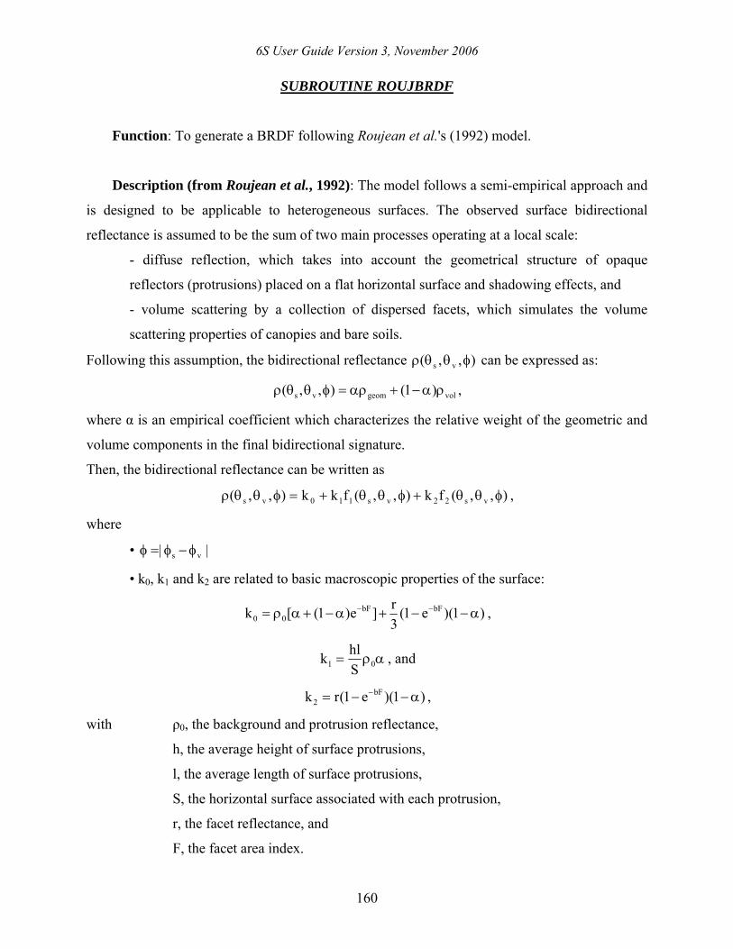
SUBROUTINE ROUJBRDF
Function: To generate a BRDF following Roujean et al.'s (1992) model.
Description (from Roujean et al., 1992): The model follows a semi-empirical approach and
is designed to be applicable to heterogeneous surfaces. The observed surface bidirectional
reflectance is assumed to be the sum of two main processes operating at a local scale:
- diffuse reflection, which takes into account the geometrical structure of opaque
reflectors (protrusions) placed on a flat horizontal surface and shadowing effects, and
- volume scattering by a collection of dispersed facets, which simulates the volume
scattering properties of canopies and bare soils.
Following this assumption, the bidirectional reflectance ),,( vs φθθρ can be expressed as:
volgeomvs )1(),,( ρα−+αρ=φθθρ ,
where α is an empirical coefficient which characterizes the relative weight of the geometric and
volume components in the final bidirectional signature.
Then, the bidirectional reflectance can be written as
),,(fk),,(fkk),,( vs22vs110vs φθθ+φθθ+=φθθρ ,
where
• || vs φ−φ=φ
• k0, k1 and k2 are related to basic macroscopic properties of the surface:
)1)(e1(3r]e)1([k bFbF
00 α−−+α−+αρ= −− ,
αρ= 01 Shlk , and
)1)(e1(rk bF2 α−−= − ,
with ρ0, the background and protrusion reflectance,
h, the average height of surface protrusions,
l, the average length of surface protrusions,
S, the horizontal surface associated with each protrusion,
r, the facet reflectance, and
F, the facet area index.
6S User Guide Version 3, November 2006
161
• f1 and f2 are simple analytic functions of the solar and view angles:
)cos()(tg)(tg2)(tg)(tg)(tg)(tg1
)(tg)(tg)sin()cos()(21),,(f
vsv2
s2
vs
vsvs1
φθθ−θ+θ+θ+θπ
−
θθφ+φφ−ππ
=φθθ, and
31)sin()cos()
2(
)cos()cos(1
34),,(f
vsvs2 −
⎭⎬⎫
⎩⎨⎧ ξ+ξξ−π
θ+θπ=φθθ
with the phase angle ξ defined as
)cos()sin()sin()cos()cos()cos( vsvs φθθ+θθ=ξ .
Parameters:
k0, k1, k2
References:
J.L. Roujean, M. Leroy, and P.Y. Deschamps, A bidirectional reflectance model of the Earth
surface for the correction of remote sensing data, Journal of Geophysical Research, 97,
20455-20468, 1992.
6S User Guide Version 3, November 2006
162
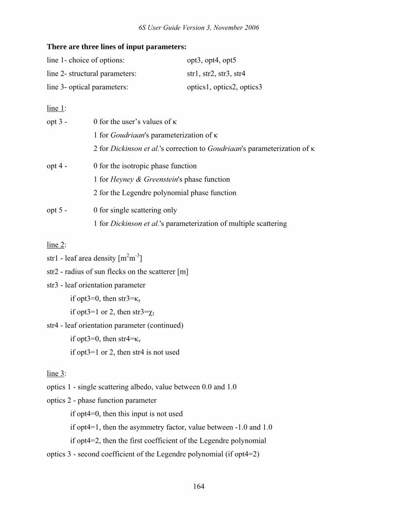
SUBROUTINE VERSBRDF
Function: To generate a BRDF following Verstraete et al.'s (1990) model.
Description (from Pinty & Verstraete, 1991): Using the basic framework previously
suggested by Hapke (1981) (see HAPKBRDF), Verstraete et al. (1990) have developed a model
for predicting the bidirectional reflectance exiting from a simple vegetation canopy. They
concentrate on the case of a fully covered, homogeneous and semi-infinite canopy made of
leaves only. With the same notations as for Hapke's model, the parametric version of the derived
model (see Pinty et al., 1990) is as follows:
1)/(H)/(H)g(P)]G(P1[4
),,,( vvssvvssv
svvss −µκµκ++
µκ+µκκω
=φθφθρ ,
where
• ω is average single-scattering albedo of particles making up the surface
• µs=cos(θs) and µv=cos(θv)
• κs and κv describe the leaf orientation distribution for the illumination and view angles,
respectively. There are 3 possible options (see below, line1-opt3)
- κs and κv are entered by the user;
- κ is obtained from Goudriaan's (1977) parameterization;
κx = Ψ1 + Ψ2 µx
with Ψ1 = 0.5 - 0.6333 χ1 - 0.33 χ12 and Ψ2 = 0.877 (1 - 2 Ψ1);
- κ is obtained from Dickinson et al.'s (1990) correction to Goudriaan's (1977)
parameterization
κx = Ψ1 + Ψ2 µx
with Ψ1 = 0.5 - 0.489 χ1 - 0.11 χ12 and Ψ2 = 1 - 2 Ψ1.
where χ1 is the leaf angle distribution function of the canopy, which varies from -0.4 for
an erectophile canopy to +0.6 for a planophile canopy. The equal probability for all leaf
orientations is given by χ1 = 0.
• Pv(G) is the function that accounts for the joint transmission of incoming and outgoing
radiation and, thereby, also for the hot spot phenomenon:
6S User Guide Version 3, November 2006
163
),,,(V11),,,(P
vvsspvvssv φθφθ+=φθφθ
with the function ),,,(V vvssp φθφθ defined by
)cos()tan()tan(2)(tan)(tanr2
)341(4),,,(V vsvsv
2s
2
v
vvvssp φ−φθθ−θ+θ
κΛµ
π−=φθφθ ,
where r is the radius of Sun flecks on the inclined scatterers [m] and Λ is the scatterer area
density of the canopy [m2m-3].
• P(g) is the average phase function of particles. There are 3 options to compute P(g) (see below,
line1-opt4):
-the case of an isotropic phase function
P(g) = 1;
- the empirical function introduced by Henyey & Greenstein (1941)
)gcos(211)g(P 2
2
Θ+Θ+Θ−
= ;
- the phase function approximated by a Legendre polynomial function
21)g(cos3L)gcos(1)g(P
2
2−
+Θ+= ,
where Θ is the asymmetry factor ranging from -1 (backward scattering) to +1, g is the
phase angle between the incoming and outgoing rays defined as
)cos()sin()sin()cos()cos()gcos( vsvsvs φ−φθθ+θθ= ,
and L2 is the second coefficient of the Legendre polynomial.
• H(x) is a function to account for multiple scattering (see below, line1-opt5):
- for single scattering
H(x) = 0;
- for multiple scattering
x)1(21
x21)x(H 2/1ω−++
= .
6S User Guide Version 3, November 2006
164
There are three lines of input parameters:
line 1- choice of options: opt3, opt4, opt5
line 2- structural parameters: str1, str2, str3, str4
line 3- optical parameters: optics1, optics2, optics3
line 1:
opt 3 - 0 for the user’s values of κ
1 for Goudriaan's parameterization of κ
2 for Dickinson et al.'s correction to Goudriaan's parameterization of κ
opt 4 - 0 for the isotropic phase function
1 for Heyney & Greenstein's phase function
2 for the Legendre polynomial phase function
opt 5 - 0 for single scattering only
1 for Dickinson et al.'s parameterization of multiple scattering
line 2:
str1 - leaf area density [m2m-3]
str2 - radius of sun flecks on the scatterer [m]
str3 - leaf orientation parameter
if opt3=0, then str3=κs
if opt3=1 or 2, then str3=χ1
str4 - leaf orientation parameter (continued)
if opt3=0, then str4=κv
if opt3=1 or 2, then str4 is not used
line 3:
optics 1 - single scattering albedo, value between 0.0 and 1.0
optics 2 - phase function parameter
if opt4=0, then this input is not used
if opt4=1, then the asymmetry factor, value between -1.0 and 1.0
if opt4=2, then the first coefficient of the Legendre polynomial
optics 3 - second coefficient of the Legendre polynomial (if opt4=2)
6S User Guide Version 3, November 2006
165
References:
R.E. Dickinson, B. Pinty, and M. Verstraete, Relating surface albedos in gcm to remotely sensed
data, Agricultural and Forest Meteorology, 52, 109-131, 1990.
J. Goudriaan, Crop micrometeorology: a simulation study (Wageningen: Wageningen Centre for
Agricultural Publishing and Documentation), 1977.
L.G. Henyey and J.L. Greenstein, Diffuse radiation in the galaxy. Astrophysical Journal, 93, 70,
1941.
B. Pinty, M. Verstraete, and R.E. Dickinson, A physical model of the bidirectional reflectance of
vegetation canopies. 1. Inversion and validation, Journal of Geophysical Research, 95,
11767-11775, 1990.
B. Pinty, and M. Verstraete, Extracting information on surface properties from bidirectional
reflectance measurements, Journal of Geophysical Research, 96, 2865-2874, 1991.
M. Verstraete, B. Pinty, and R.E. Dickinson, A physical model of the bidirectional reflectance of
vegetation canopies. 1. Theory, Journal of Geophysical Research, 95, 11755-11765, 1990.
6S User Guide Version 3, November 2006
166
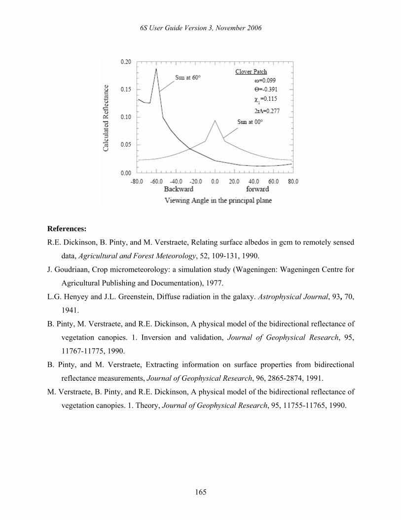
SUBROUTINE WALTBRDF
Function: To generate a BRDF following Walthall et al.'s (1985) model.
Description (from Walthall et al., 1985): Using a deterministic model, Walthall et al.
(1985) have simulated different canopy reflectance distributions. The 2-D contours of these
distributions appeared to be similar to the shape of the Pascal limacon. Using the simple limacon
equation, Walthall et al. checked other equation forms trying to fit the 3-D reflectance surface
directly. They found satisfactory results with the following equation:
c)cos(ba),,,( svv2
vvsvs +φ−φθ+θ=φφθθρ
where ρ is the reflectance at given view zenith θv and view azimuth vφ angles, and a, b, and c
are coefficients derived using a linear least-squares fitting procedure.
The model has to be slightly modified to match the reciprocity principle. The reflectance is
written:
c)cos(b)('aa),,,( svvs2
v2
s2
v2
svsvs +φ−φθθ+θ+θ+θθ=φφθθρ .
Parameters:
a, a', b, c
Reference:
C.L. Walthall, J.M. Norman, J.M. Welles, G. Campbell, and B.L. Blad, Simple equation to
approximate the bidirectional reflectance from vegetative canopies and bare soil surfaces,
Applied Optics, 24(3), 383-387, 1985.
6S User Guide Version 3, November 2006
167
SUBROUTINE AKBRDF
Function: To generate a BRDF following Kuusk's (1994) model.
Description (from Kuusk, 1994, 1995): The single scattering radiance of a canopy layer
with the height H is
dz)r,r,z(p)r,r()z(uF
I 0
H
00L
0
001c ∫ Γ
πµµµ
= (1)
where πµ /F 00 is the intensity of the incident direct flux on a horizontal surface, uL is the leaf
area density, Γ(r0,r) is the phase function of single scattering, p(z,r0,r) is the bidirectional gap
probability inside a canopy at the level z in directions ),(r 000 φθ and ),(r φθ , and µ0 and µ are the
respective cosines.
The phase function Γ=ΓD+ ΓSP and bidirectional gap probability p(z,r0,r) = p(r0)p(r)CHS(r0,r)
are functions of the leaf angle distribution gL(θL). Here ΓD is the phase function of diffuse
scattering of lambertian leaves (see Eq. (10) of subroutine IAPIBRDF), and ΓSP is the phase
function of Fresnel reflection on the leaf surface. The phase function of specular reflection is
corrected for the leaf hair and surface roughness (Nilson & Kuusk, 1989). The hot spot factor
⎪⎭
⎪⎬⎫
⎪⎩
⎪⎨⎧
⎥⎦
⎤⎢⎣
⎡⎟⎟⎠
⎞⎜⎜⎝
⎛ ∆−−
∆µµ=α
L
21
21
LH
21
)2(L
)1(L
HS s)r,r(exp1
)r,r(sLGGexp),H(C (2)
considers for the finite leaf size Ls . Here )r,r( 21∆ = )/(cos211 2122
21 µµα−µ+µ is the geometry
factor, and π-α is the scattering angle.
The function GL(r) is given by Eq. (9) of subroutine IAPIBRDF. For the cases of a spherical
orientation of leaves and fixed angle of leaves, exact analytical expressions for the phase
function Γ and G-function were obtained by T. Nilson (see Ross, 1981). In case of an elliptical
leaf angle distribution :
)(cos1B)(g mL22
gLL θ−θε−=θ , (3)
the analytical approximations for the G-function and phase function Γ were obtained by Kuusk
(1995). Here the eccentricity ε and modal inclination θm are the LAD parameters, Bg is a
normalizing factor.
6S User Guide Version 3, November 2006
168
Single scattering from soil is given by
)r,r,H()r,r(I 00soilIsoil ρρ= (4)
where ρsoil(r0,r) is the bidirectional reflectance of soil. The parabolic approximation of Walthall
et al. (1985) is applied for the BRDF of soil ρsoil(r0,r).
Multiple scattering of radiation on foliage and soil is defined by Schwarzschild's
approximation (Nilson & Kuusk, 1989).
The wavelength-dependent optical parameters of the CR model are calculated with
Jacquemoud & Baret PROSPECT model (1990) for leaves, and with Price's (1990) base
functions (1990) for soil.
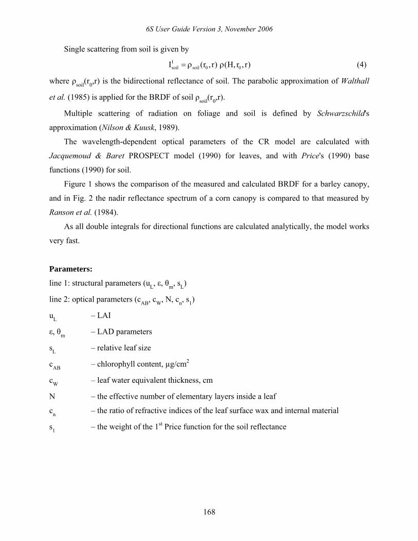
Figure 1 shows the comparison of the measured and calculated BRDF for a barley canopy,
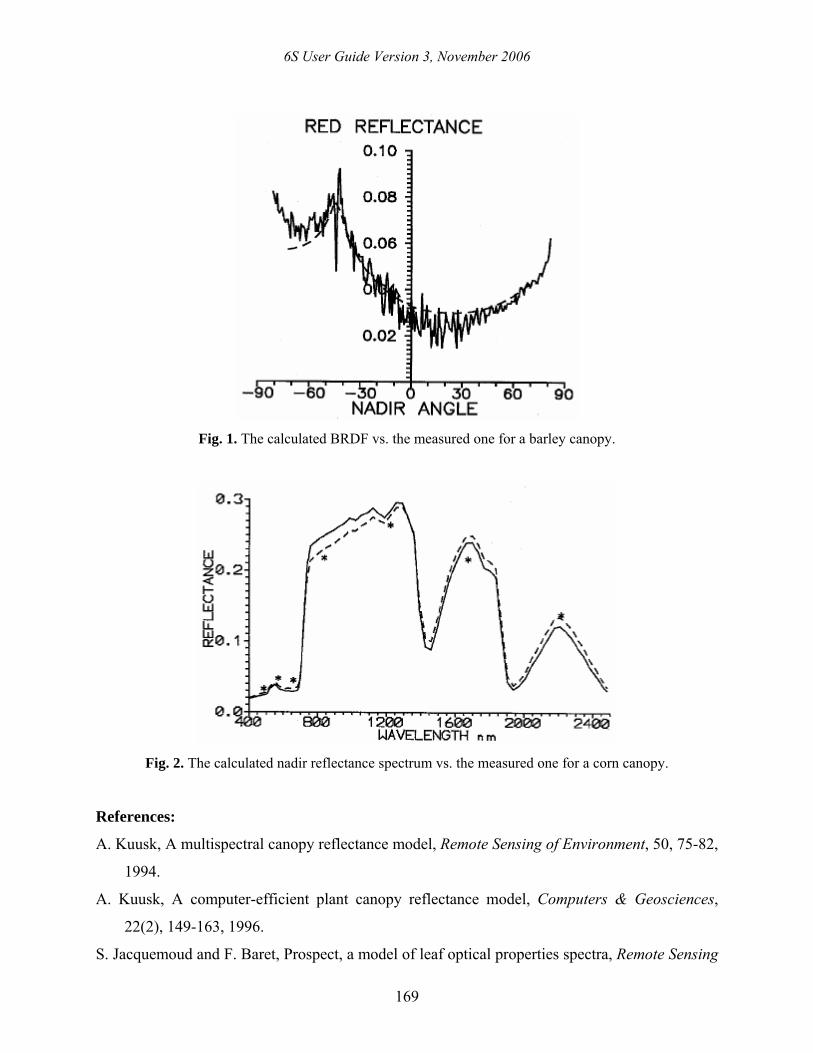
and in Fig. 2 the nadir reflectance spectrum of a corn canopy is compared to that measured by
Ranson et al. (1984).
As all double integrals for directional functions are calculated analytically, the model works
very fast.
Parameters:
line 1: structural parameters (uL, ε, θm, sL)
line 2: optical parameters (cAB, cW, N, cn, s1)
uL – LAI
ε, θm – LAD parameters
sL – relative leaf size
cAB – chlorophyll content, µg/cm2
cW – leaf water equivalent thickness, cm
N – the effective number of elementary layers inside a leaf
cn – the ratio of refractive indices of the leaf surface wax and internal material
s1 – the weight of the 1st Price function for the soil reflectance
6S User Guide Version 3, November 2006
169
Fig. 1. The calculated BRDF vs. the measured one for a barley canopy.
Fig. 2. The calculated nadir reflectance spectrum vs. the measured one for a corn canopy.
References:
A. Kuusk, A multispectral canopy reflectance model, Remote Sensing of Environment, 50, 75-82,
1994.
A. Kuusk, A computer-efficient plant canopy reflectance model, Computers & Geosciences,
22(2), 149-163, 1996.
S. Jacquemoud and F. Baret, Prospect, a model of leaf optical properties spectra, Remote Sensing
6S User Guide Version 3, November 2006
170
of Environment, 34, 75-91, 1990
T. Nilson and A. Kuusk, A reflectance model for the homogeneous plant canopy and its
inversion, Remote Sensing of Environment, 27, 157-167, 1989.
J.C. Price, On the information content of soil reflectance spectra, Remote Sensing of
Environment, 33, 113-121, 1990.
J. Ross, The radiation regime and architecture of plant stands, W. Junk, The Hague, 391 p., 1981.
C.L. Walthall, J.M. Norman, M.J. Welles, G. Campbell, and B.L. Blad, Simple equation to
approximate the bidirectional reflectance from vegetative canopies and bare soil surfaces,
Applied Optics, 24(3), 383-387, 1985.
6S User Guide Version 3, November 2006
171
SUBROUTINE AKLABE
Function: To calculate the spherical albedo using the BRDF computed by Kuusk’s (1994)
model.
Description: This subroutine is based on the same physical principles as the other 6SV
subroutines used for spherical albedo calculations; the only difference is in the programming
method. AKALBE is a part of the “Multispectral Canopy Reflectance Model” package which
was written by A. Kuusk himself in 1994 and directly incorporated into 6S soon afterwards.
References:
A. Kuusk, A multispectral canopy reflectance model, Remote Sensing of Environment, 50, 75-82,
1994.
A. Kuusk, A computer-efficient plant canopy reflectance model, Computers & Geosciences,
22(2), 149-163, 1996.
6S User Guide Version 3, November 2006
172
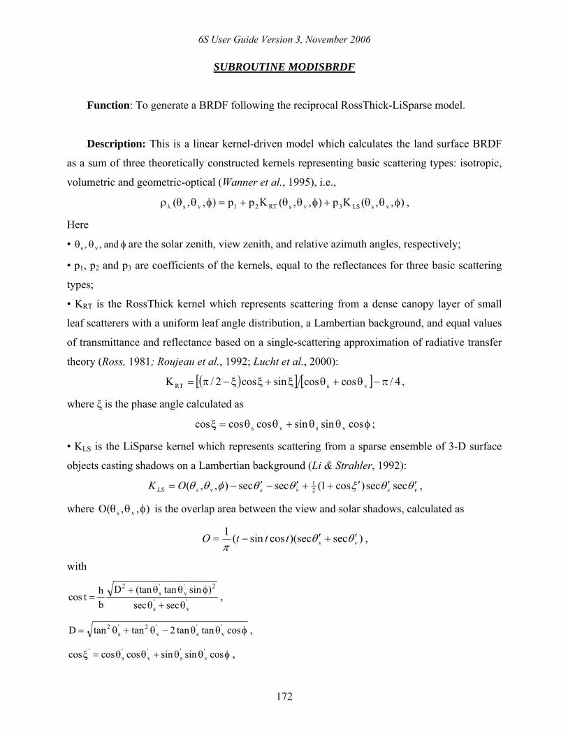
SUBROUTINE MODISBRDF
Function: To generate a BRDF following the reciprocal RossThick-LiSparse model.
Description: This is a linear kernel-driven model which calculates the land surface BRDF
as a sum of three theoretically constructed kernels representing basic scattering types: isotropic,
volumetric and geometric-optical (Wanner et al., 1995), i.e.,
),,(Kp),,(Kpp),,( vsLS3vsRT21vs φθθ+φθθ+=φθθρλ ,
Here
• φθθ and,, vs are the solar zenith, view zenith, and relative azimuth angles, respectively;
• p1, p2 and p3 are coefficients of the kernels, equal to the reflectances for three basic scattering
types;
• KRT is the RossThick kernel which represents scattering from a dense canopy layer of small
leaf scatterers with a uniform leaf angle distribution, a Lambertian background, and equal values
of transmittance and reflectance based on a single-scattering approximation of radiative transfer
theory (Ross, 1981; Roujeau et al., 1992; Lucht et al., 2000):
( )[ ] [ ] 4/coscossincos2/K vsRT π−θ+θξ+ξξ−π= ,
where ξ is the phase angle calculated as
φθθ+θθ=ξ cossinsincoscoscos vsvs ;
• KLS is the LiSparse kernel which represents scattering from a sparse ensemble of 3-D surface
objects casting shadows on a Lambertian background (Li & Strahler, 1992):
vsvsvsLS OK θθξθθφθθ ′′′++′−′−= secsec)cos1(secsec),,( 21 ,
where ),,(O vs φθθ is the overlap area between the view and solar shadows, calculated as
)sec)(seccossin(1vstttO θθ
π′+′−= ,
with
'v
's
2'v
's
2
secsec)sintan(tanD
bhtcos
θ+θφθθ+
= ,
φθθ−θ+θ= costantan2tantanD 'v
's
'v
2's
2 ,
φθθ+θθ=ξ cossinsincoscoscos 'v
's
'v
's
' ,
6S User Guide Version 3, November 2006
173
⎟⎠⎞
⎜⎝⎛ θ=θ⎟
⎠⎞
⎜⎝⎛ θ=θ −−
v1'
vs1'
s tanrbtanand,tan
rbtan .
The ratios h/b and b/r are the dimensionless crown relative height and shape parameters which
should be preselected. The MODIS products assume h/b=2 and b/r=1, i.e., the spherical crowns
are separated from the ground by half their diameter (Lucht et al., 2000).
References:
W. Wanner, X. Li and A.H. Strahler, On the derivation of kernels for kernel-driven models of
bidirectional reflectance, Journal of Geophysical Research, 100(D10), 21077–21090, 1995.
J.K. Ross, The radiation regime and architecture of plant stands, Dr. W. Junk, Norwell, MA,
392 p., 1981.
J.L. Roujean, M. Leroy, and P.Y. Deschamps, A bidirectional reflectance model of the Earth's
surface for the correction of remote sensing data, Journal of Geophysical Research,
97(D18), 20455–20468, 1992.
X. Li and A.H. Strahler, Geometric-optical bidirectional reflectance modeling of the discrete
crown vegetation canopy: effect of crown shape and mutual shadowing, IEEE Transactions
on Geoscience and Remote Sensing, 30(2), 276-292, 1992.
W. Lucht, C.B. Schaaf, and A.H. Strahler, An algorithm for the retrieval of albedo from space
using semiempirical BRDF models, IEEE Transactions on Geoscience and Remote Sensing,
38(2), 977-998, 2000.
6S User Guide Version 3, November 2006
174
SUBROUTINE MODISALBE
Function: To calculate the spherical albedo using the BRDF values computed by the
MODISBRDF subroutine.
Description: The spherical albedo s is calculated as
s = p1 + p2 · 0.189184 – p3 · 1.377622,
where p1, p2 and p3 are coefficients of the kernels, representing the reflectances of the isotropic,
radiative transfer-type volumetric, and geometric-optical surface (see subroutine MODISBRDF).
6S User Guide Version 3, November 2006
175
DESCRIPTION OF THE SUBROUTINES USED
TO UPDATE THE ATMOSPHERIC PROFILE
(AIRPLANE OR ELEVATED TARGET SIMULATIONS)
6S User Guide Version 3, November 2006
176
SUBROUTINE PRESPLANE
Function: Update the atmospheric profile (P(z),T(z),H2O(z),O3(z)) if the observer is on-
board an aircraft.
Description: Given the altitude or pressure at the aircraft level as an input, the first task is to
compute the altitude (if the pressure has been entered) or pressure (if the altitude has been
entered) at the plane level. Then, a new atmospheric profile is created (Pp,Tp,H2Op,O3p), for
which the last level is located at the plane altitude. This profile is used in the gaseous absorption
computation (subroutine ABSTRA) for the path from target to sensor (upward transmission).
The ozone and water vapor integrated content of the "plane" atmospheric profile are also outputs
of this subroutine. The last output is the proportion of molecules below the plane level, which is
used in scattering computations (subroutines OSPOL and ISO).
6S User Guide Version 3, November 2006
177
SUBROUTINE PRESSURE
Function: Update the atmospheric profile (P(z),T(z),H2O(z),O3(z)) if the target is not at the
sea level.
Description: Given the altitude of the target in km as an input, we transform the original
atmospheric profile (pressure, temperature, water vapor, ozone) so that the first level of the new
profile is the one at the target altitude. We also compute the new integrated content of water
vapor and ozone, which is used as an output in computations when the user chooses to enter a
specific amount of H2O and O3.
6S User Guide Version 3, November 2006
178
DESCRIPTION OF THE SUBROUTINES USED TO READ THE DATA
6S User Guide Version 3, November 2006
179
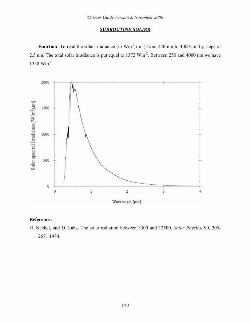
SUBROUTINE SOLIRR
Function: To read the solar irradiance (in Wm-2µm-1) from 250 nm to 4000 nm by steps of
2.5 nm. The total solar irradiance is put equal to 1372 Wm-2. Between 250 and 4000 nm we have
1358 Wm-2.
Reference:
H. Neckel, and D. Labs, The solar radiation between 3300 and 12500, Solar Physics, 90, 205-
258, 1984.
6S User Guide Version 3, November 2006
180
SUBROUTINE VARSOL
Function: To take into account the variation of the solar constant as a function of the Julian
day.
Description: We apply a simple multiplicative factor DS to the solar constant CS. DS is
written as
2S )Mcose1(1D
−=
with
180)4J(9856.0M π
−=
where e = 0.01673 and J is the Julian day.
Reference:
G.W. Paltridge, and C.M.R. Platt, Radiative processes in meteorology and climatology, Elsevier
Publishing, New-York, 1977.
6S User Guide Version 3, November 2006
181
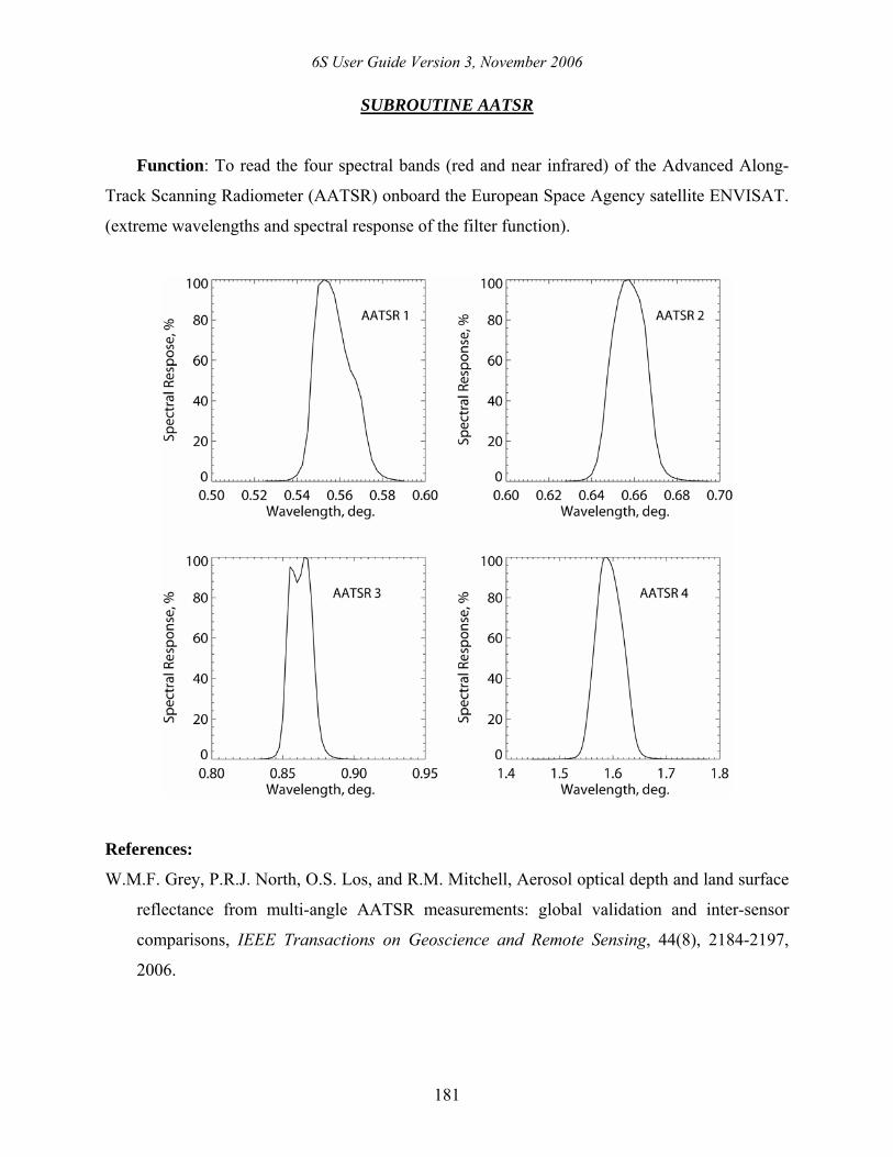
SUBROUTINE AATSR
Function: To read the four spectral bands (red and near infrared) of the Advanced Along-
Track Scanning Radiometer (AATSR) onboard the European Space Agency satellite ENVISAT.
(extreme wavelengths and spectral response of the filter function).
References:
W.M.F. Grey, P.R.J. North, O.S. Los, and R.M. Mitchell, Aerosol optical depth and land surface
reflectance from multi-angle AATSR measurements: global validation and inter-sensor
comparisons, IEEE Transactions on Geoscience and Remote Sensing, 44(8), 2184-2197,
2006.
6S User Guide Version 3, November 2006
182
A.G. O'Carroll, J.G. Watts, L.A. Horrocks, R.W. Saunders, and N.A. Rayner, Validation of the
AATSR Meteo product Sea Surface Temperature, Journal of Atmospheric and Oceanic
Technology, 23(5), 711-726, 2006.
Links:
http://envisat.esa.int/instruments/aatsr/
http://www.atsr.rl.ac.uk/documentation/index.shtml
http://www.leos.le.ac.uk/aatsr/
6S User Guide Version 3, November 2006
183
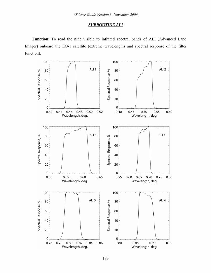
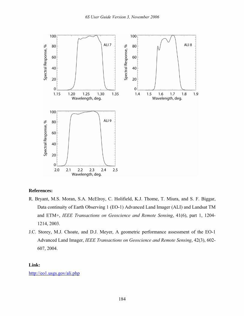
SUBROUTINE ALI
Function: To read the nine visible to infrared spectral bands of ALI (Advanced Land
Imager) onboard the EO-1 satellite (extreme wavelengths and spectral response of the filter
function).
6S User Guide Version 3, November 2006
184
References:
R. Bryant, M.S. Moran, S.A. McElroy, C. Holifield, K.J. Thome, T. Miura, and S. F. Biggar,
Data continuity of Earth Observing 1 (EO-1) Advanced Land Imager (ALI) and Landsat TM
and ETM+, IEEE Transactions on Geoscience and Remote Sensing, 41(6), part 1, 1204-
1214, 2003.
J.C. Storey, M.J. Choate, and D.J. Meyer, A geometric performance assessment of the EO-1
Advanced Land Imager, IEEE Transactions on Geoscience and Remote Sensing, 42(3), 602-
607, 2004.
Link:
http://eo1.usgs.gov/ali.php
6S User Guide Version 3, November 2006
185
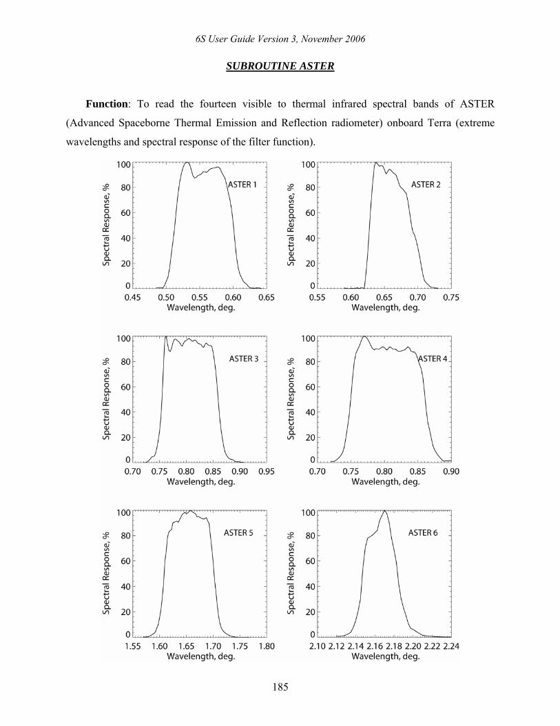
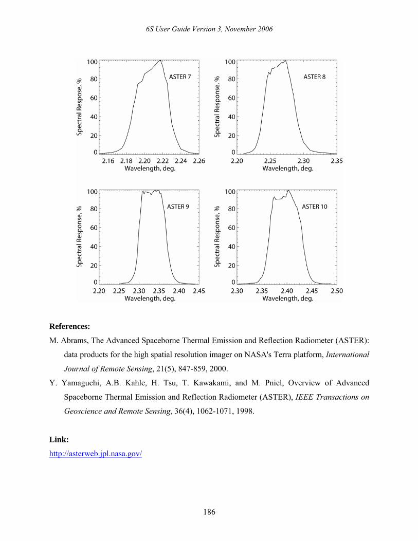
SUBROUTINE ASTER
Function: To read the fourteen visible to thermal infrared spectral bands of ASTER
(Advanced Spaceborne Thermal Emission and Reflection radiometer) onboard Terra (extreme
wavelengths and spectral response of the filter function).
6S User Guide Version 3, November 2006
186
References:
M. Abrams, The Advanced Spaceborne Thermal Emission and Reflection Radiometer (ASTER):
data products for the high spatial resolution imager on NASA's Terra platform, International
Journal of Remote Sensing, 21(5), 847-859, 2000.
Y. Yamaguchi, A.B. Kahle, H. Tsu, T. Kawakami, and M. Pniel, Overview of Advanced
Spaceborne Thermal Emission and Reflection Radiometer (ASTER), IEEE Transactions on
Geoscience and Remote Sensing, 36(4), 1062-1071, 1998.
Link:
http://asterweb.jpl.nasa.gov/
6S User Guide Version 3, November 2006
187
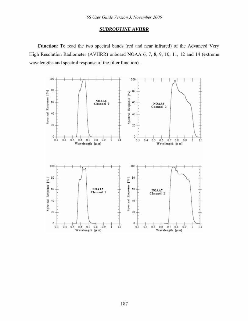
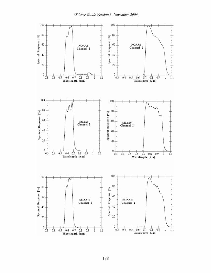
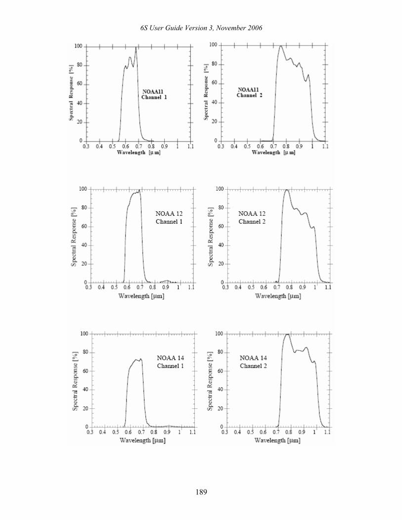
SUBROUTINE AVHRR
Function: To read the two spectral bands (red and near infrared) of the Advanced Very
High Resolution Radiometer (AVHRR) onboard NOAA 6, 7, 8, 9, 10, 11, 12 and 14 (extreme
wavelengths and spectral response of the filter function).
6S User Guide Version 3, November 2006
188
6S User Guide Version 3, November 2006
189
6S User Guide Version 3, November 2006
190
References:
C.T. Due, Optical-mechanical active/passive imaging Systems - Volume II, Report number
153200-2-TIII- ERIM Infrared information and Analysis Center, P.O. BOX 8518, Ann.
Arbor., MI.98107, 1982.
NOAA Polar Orbiter Data User’s Guide, U.S. Dept. of Commerce, NOAA, National
Environment Satellite, National Climatic Data Center, Satellite Data Service Division,
World Weather Building, Room 100, Washington D.C., 202333, USA, 1985.
S.R. Schneider and D.F. McGinnis, The NOAA/AVHRR: A new satellite sensor for monitoring
crop growth, Proceedings of the Eighth International Symposium on Machine processing of
remotely sensed data, Purdue University, Indiana, 250-281, 1982.
Links:
http://www2.ncdc.noaa.gov/docs/klm/html/c3/sec3-1.htm
http://edc.usgs.gov/products/satellite/avhrr.html
6S User Guide Version 3, November 2006
191
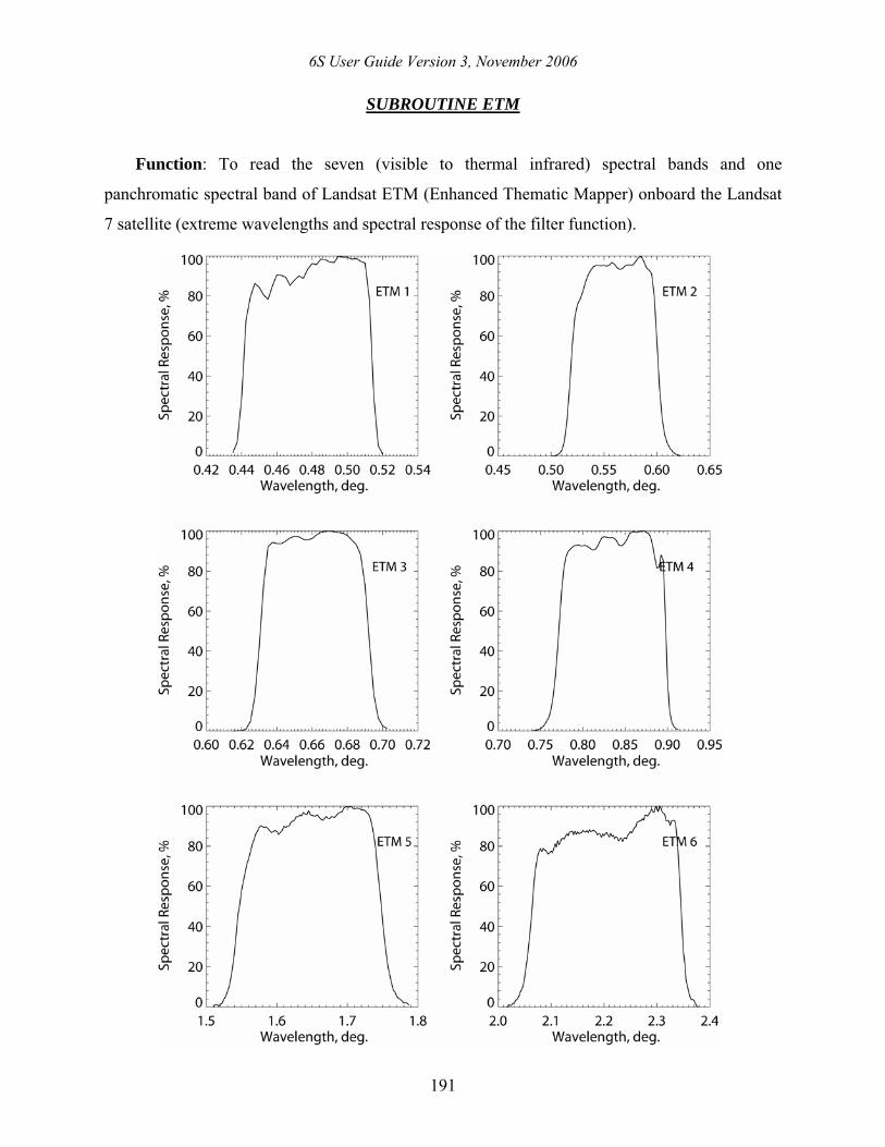
SUBROUTINE ETM
Function: To read the seven (visible to thermal infrared) spectral bands and one
panchromatic spectral band of Landsat ETM (Enhanced Thematic Mapper) onboard the Landsat
7 satellite (extreme wavelengths and spectral response of the filter function).
6S User Guide Version 3, November 2006
192
References:
S. Liang, H. Fang, and M. Chen, Atmospheric correction of Landsat ETM+ land surface
imagery. Part I: Methods, IEEE Transactions on Geoscience and Remote Sensing, 39(11),
2490-2498, 2001.
S. Liang, H. Fang, J.T. Morisette, M. Chen, C.J. Shuey, C.L. Walthall, and C.S.T. Daughtry,
Atmospheric correction of Landsat ETM+ land surface imagery. Part II: Validation and
applications, IEEE Transactions on Geoscience and Remote Sensing, 40(12), 2736-2746.
Link:
http://edc.usgs.gov/products/satellite/landsat7.html
6S User Guide Version 3, November 2006
193
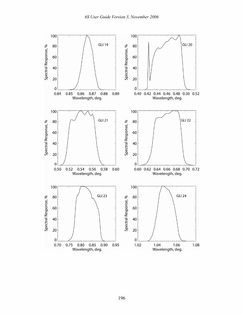
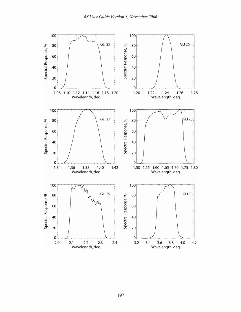
SUBROUTINE GLI
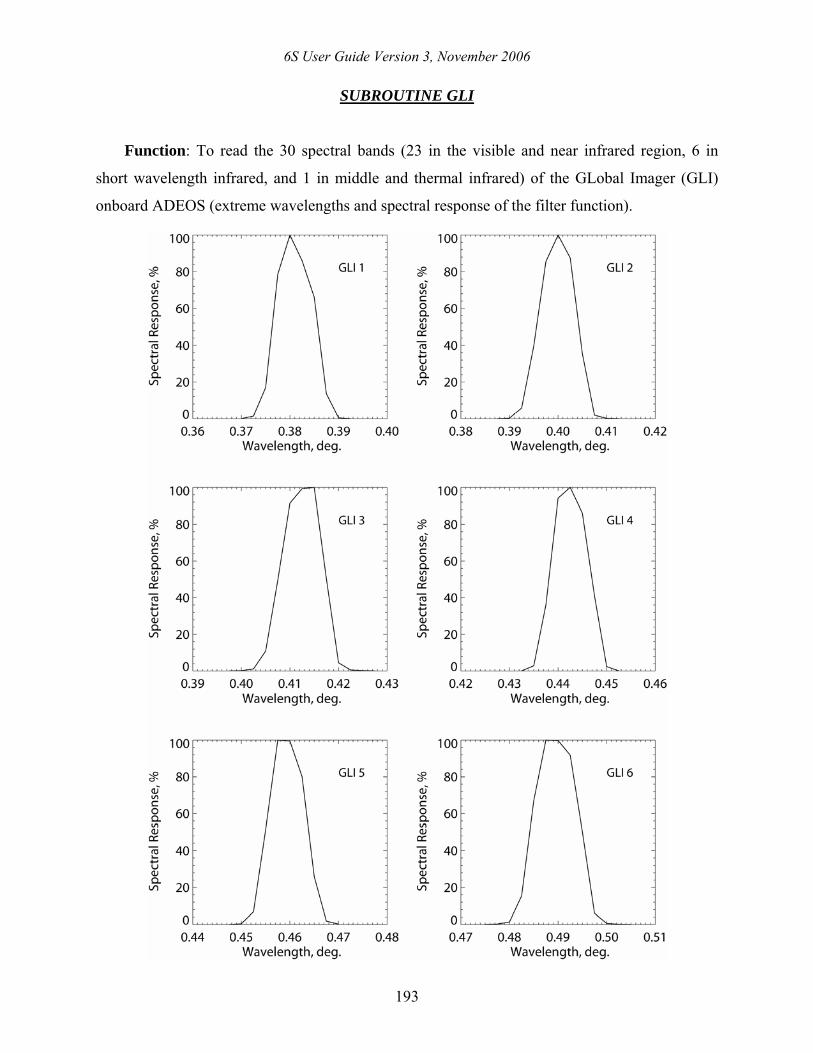
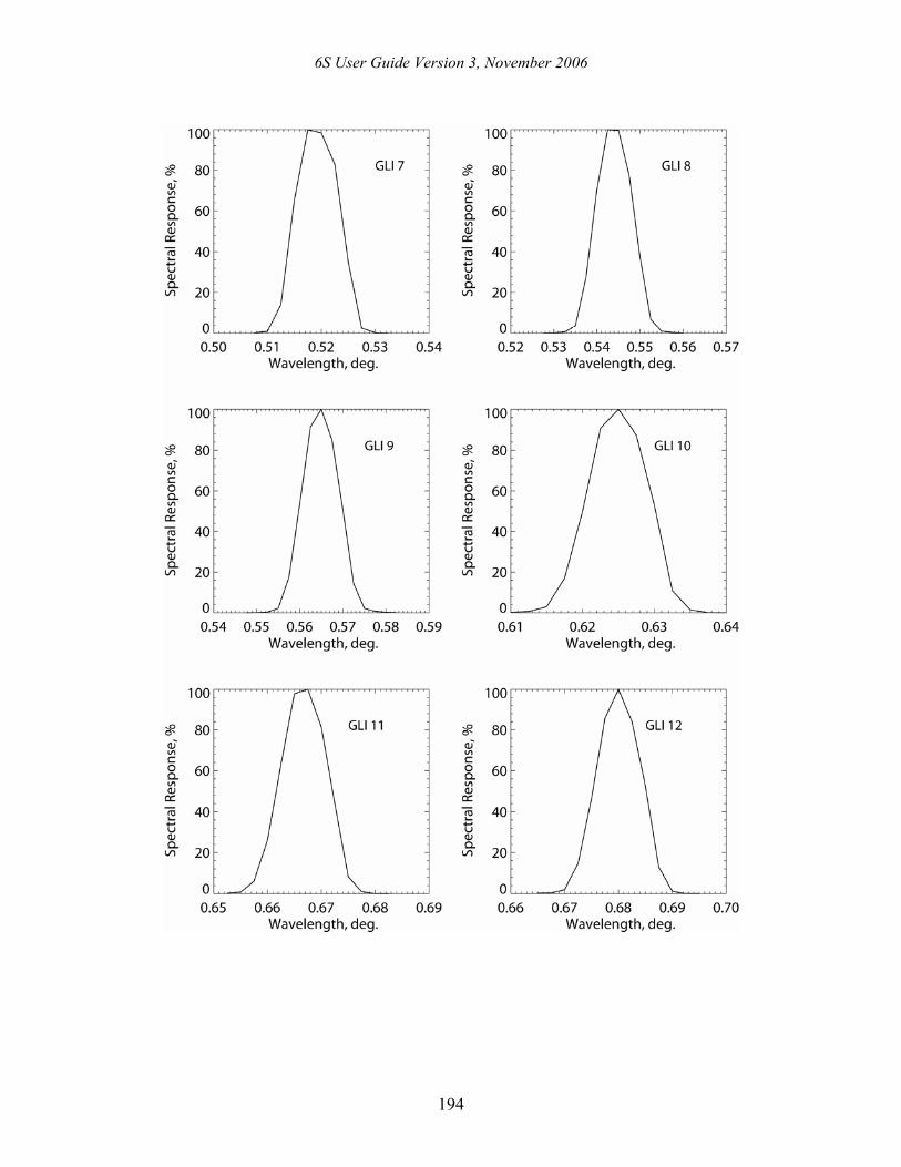
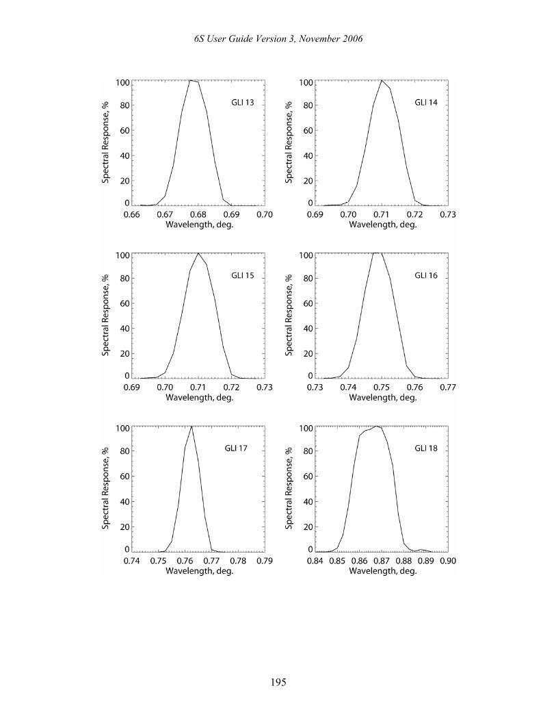
Function: To read the 30 spectral bands (23 in the visible and near infrared region, 6 in
short wavelength infrared, and 1 in middle and thermal infrared) of the GLobal Imager (GLI)
onboard ADEOS (extreme wavelengths and spectral response of the filter function).
6S User Guide Version 3, November 2006
194
6S User Guide Version 3, November 2006
195
6S User Guide Version 3, November 2006
196
6S User Guide Version 3, November 2006
197

6S User Guide Version 3, November 2006
198
Reference:
M. Yoshida, H. Murakami, Y. Mitomi, M. Hori, K.J. Thome, D.K. Clark, and H. Fukushima,
Vicarious calibration of GLI by ground observation data, IEEE Transactions on Geoscience
and Remote Sensing, 43(10), 2167 – 2176, 2005.
Links:
http://www.eoc.jaxa.jp/satellite/sendata/gli_e.html
http://suzaku.eorc.jaxa.jp/GLI/alg/alg_des.html (ATBD)
6S User Guide Version 3, November 2006
199
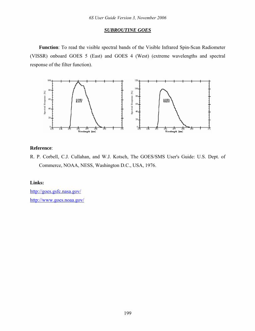
SUBROUTINE GOES
Function: To read the visible spectral bands of the Visible Infrared Spin-Scan Radiometer
(VISSR) onboard GOES 5 (East) and GOES 4 (West) (extreme wavelengths and spectral
response of the filter function).
Reference:
R. P. Corbell, C.J. Cullahan, and W.J. Kotsch, The GOES/SMS User's Guide: U.S. Dept. of
Commerce, NOAA, NESS, Washington D.C., USA, 1976.
Links:
http://goes.gsfc.nasa.gov/
http://www.goes.noaa.gov/
6S User Guide Version 3, November 2006
200
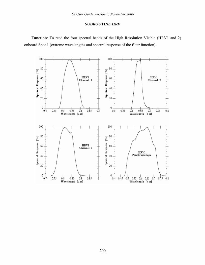
SUBROUTINE HRV
Function: To read the four spectral bands of the High Resolution Visible (HRV1 and 2)
onboard Spot 1 (extreme wavelengths and spectral response of the filter function).
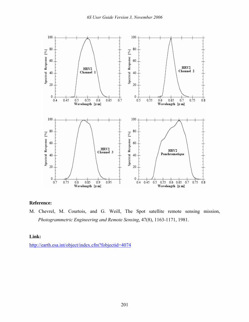
6S User Guide Version 3, November 2006
201
Reference:
M. Chevrel, M. Courtois, and G. Weill, The Spot satellite remote sensing mission,
Photogrammetric Engineering and Remote Sensing, 47(8), 1163-1171, 1981.
Link:
http://earth.esa.int/object/index.cfm?fobjectid=4074
6S User Guide Version 3, November 2006
202
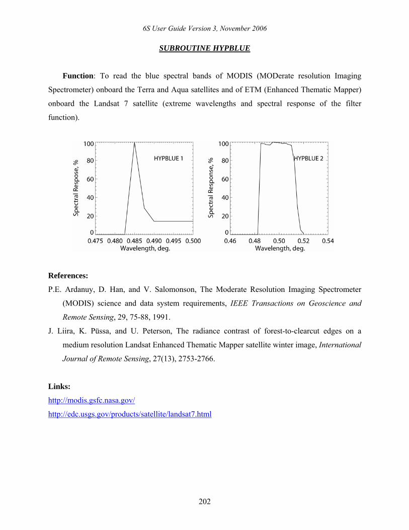
SUBROUTINE HYPBLUE
Function: To read the blue spectral bands of MODIS (MODerate resolution Imaging
Spectrometer) onboard the Terra and Aqua satellites and of ETM (Enhanced Thematic Mapper)
onboard the Landsat 7 satellite (extreme wavelengths and spectral response of the filter
function).
References:
P.E. Ardanuy, D. Han, and V. Salomonson, The Moderate Resolution Imaging Spectrometer
(MODIS) science and data system requirements, IEEE Transactions on Geoscience and
Remote Sensing, 29, 75-88, 1991.
J. Liira, K. Püssa, and U. Peterson, The radiance contrast of forest-to-clearcut edges on a
medium resolution Landsat Enhanced Thematic Mapper satellite winter image, International
Journal of Remote Sensing, 27(13), 2753-2766.
Links:
http://modis.gsfc.nasa.gov/
http://edc.usgs.gov/products/satellite/landsat7.html
6S User Guide Version 3, November 2006
203
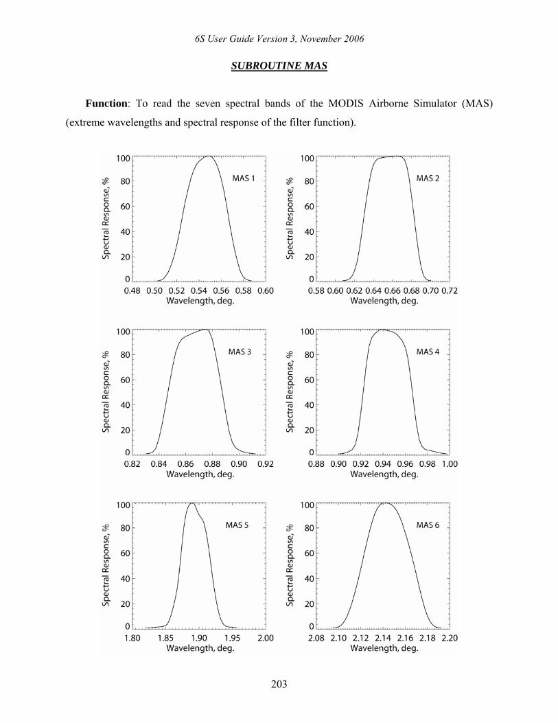
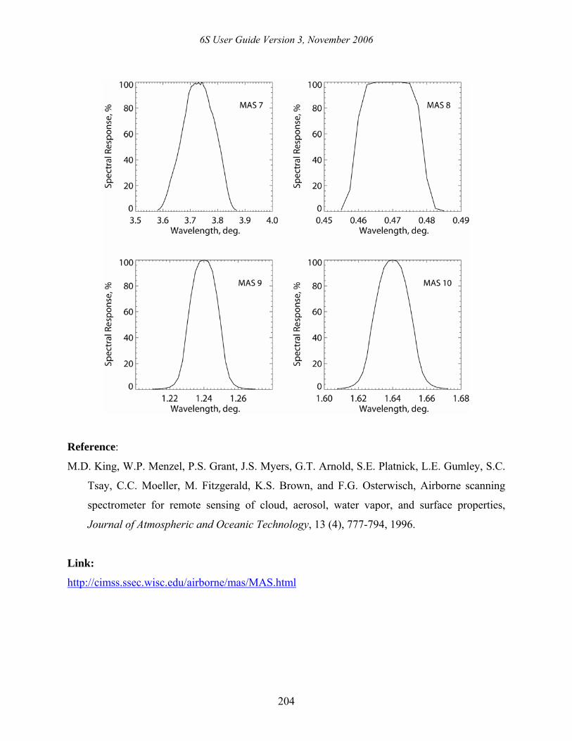
SUBROUTINE MAS
Function: To read the seven spectral bands of the MODIS Airborne Simulator (MAS)
(extreme wavelengths and spectral response of the filter function).
6S User Guide Version 3, November 2006
204
Reference:
M.D. King, W.P. Menzel, P.S. Grant, J.S. Myers, G.T. Arnold, S.E. Platnick, L.E. Gumley, S.C.
Tsay, C.C. Moeller, M. Fitzgerald, K.S. Brown, and F.G. Osterwisch, Airborne scanning
spectrometer for remote sensing of cloud, aerosol, water vapor, and surface properties,
Journal of Atmospheric and Oceanic Technology, 13 (4), 777-794, 1996.
Link:
http://cimss.ssec.wisc.edu/airborne/mas/MAS.html
6S User Guide Version 3, November 2006
205
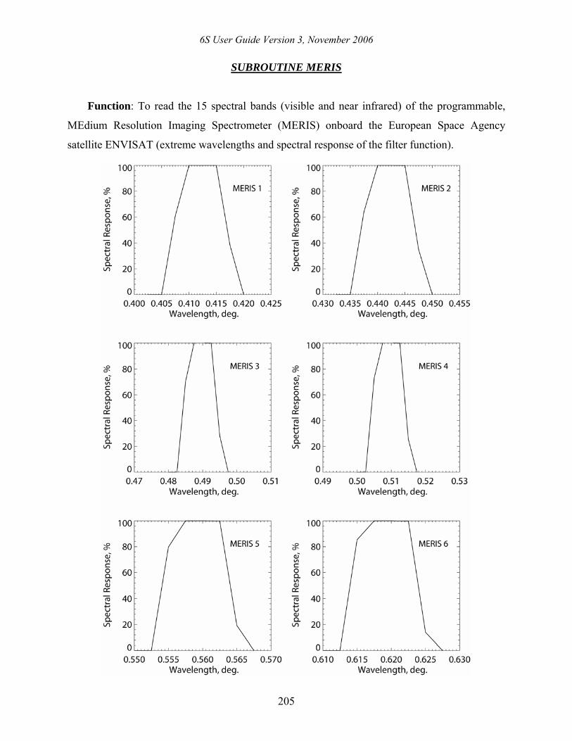
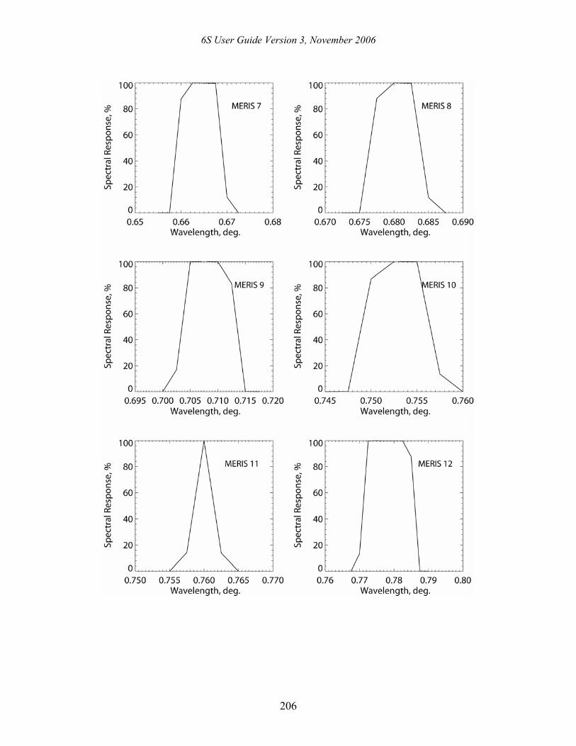
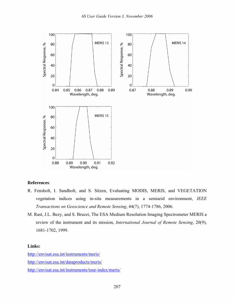
SUBROUTINE MERIS
Function: To read the 15 spectral bands (visible and near infrared) of the programmable,
MEdium Resolution Imaging Spectrometer (MERIS) onboard the European Space Agency
satellite ENVISAT (extreme wavelengths and spectral response of the filter function).
6S User Guide Version 3, November 2006
206
6S User Guide Version 3, November 2006
207
References:
R. Fensholt, I. Sandholt, and S. Sitzen, Evaluating MODIS, MERIS, and VEGETATION
vegetation indices using in-situ measurements in a semiarid environment, IEEE
Transactions on Geoscience and Remote Sensing, 44(7), 1774-1786, 2006.
M. Rast, J.L. Bezy, and S. Bruzzi, The ESA Medium Resolution Imaging Spectrometer MERIS a
review of the instrument and its mission, International Journal of Remote Sensing, 20(9),
1681-1702, 1999.
Links:
http://envisat.esa.int/instruments/meris/
http://envisat.esa.int/dataproducts/meris/
http://envisat.esa.int/instruments/tour-index/meris/
6S User Guide Version 3, November 2006
208
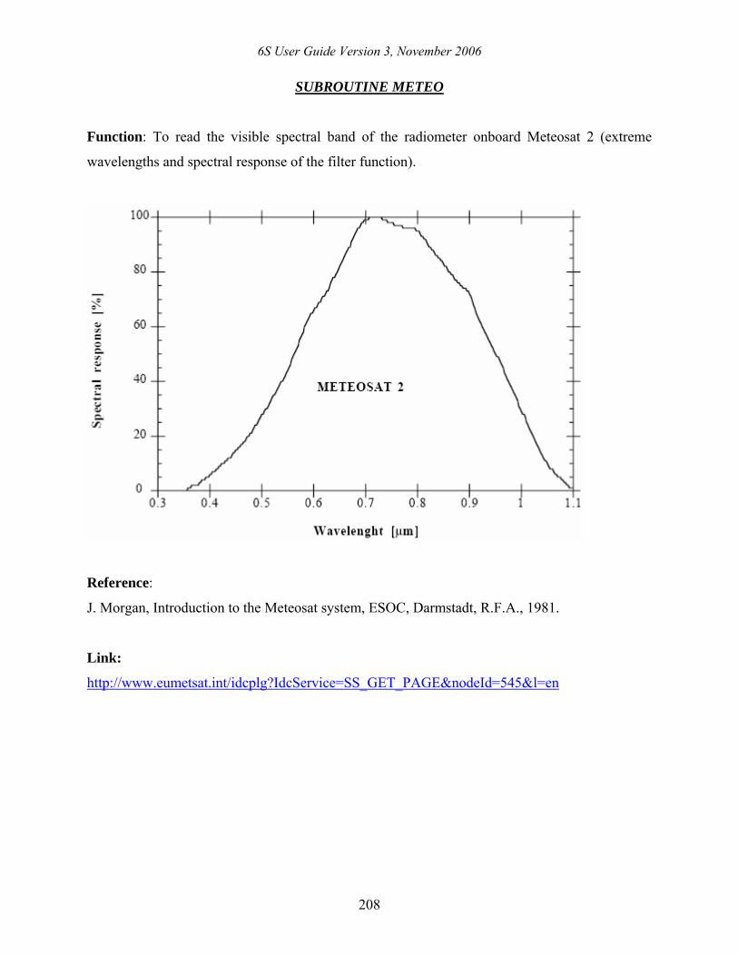
SUBROUTINE METEO
Function: To read the visible spectral band of the radiometer onboard Meteosat 2 (extreme
wavelengths and spectral response of the filter function).
Reference:
J. Morgan, Introduction to the Meteosat system, ESOC, Darmstadt, R.F.A., 1981.
Link:
http://www.eumetsat.int/idcplg?IdcService=SS_GET_PAGE&nodeId=545&l=en
6S User Guide Version 3, November 2006
209
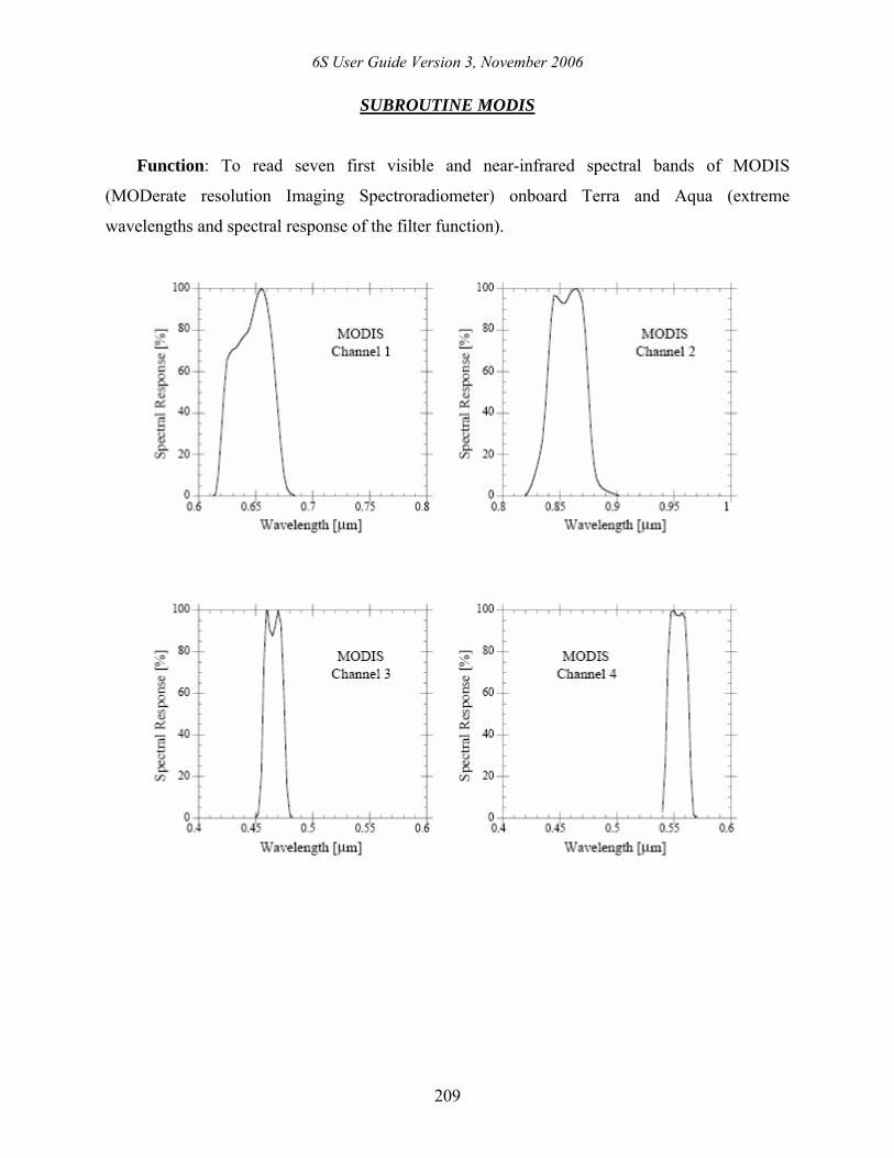
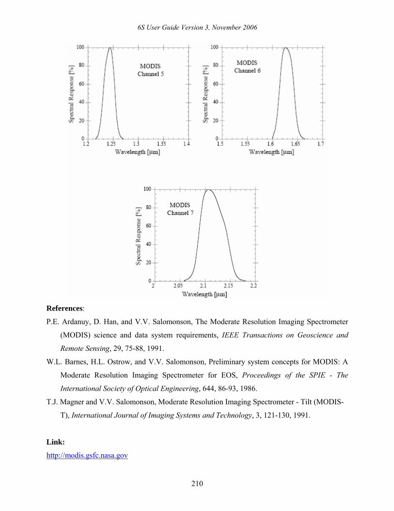
SUBROUTINE MODIS
Function: To read seven first visible and near-infrared spectral bands of MODIS
(MODerate resolution Imaging Spectroradiometer) onboard Terra and Aqua (extreme
wavelengths and spectral response of the filter function).
6S User Guide Version 3, November 2006
210
References:
P.E. Ardanuy, D. Han, and V.V. Salomonson, The Moderate Resolution Imaging Spectrometer
(MODIS) science and data system requirements, IEEE Transactions on Geoscience and
Remote Sensing, 29, 75-88, 1991.
W.L. Barnes, H.L. Ostrow, and V.V. Salomonson, Preliminary system concepts for MODIS: A
Moderate Resolution Imaging Spectrometer for EOS, Proceedings of the SPIE - The
International Society of Optical Engineering, 644, 86-93, 1986.
T.J. Magner and V.V. Salomonson, Moderate Resolution Imaging Spectrometer - Tilt (MODIS-
T), International Journal of Imaging Systems and Technology, 3, 121-130, 1991.
Link:
http://modis.gsfc.nasa.gov
6S User Guide Version 3, November 2006
211
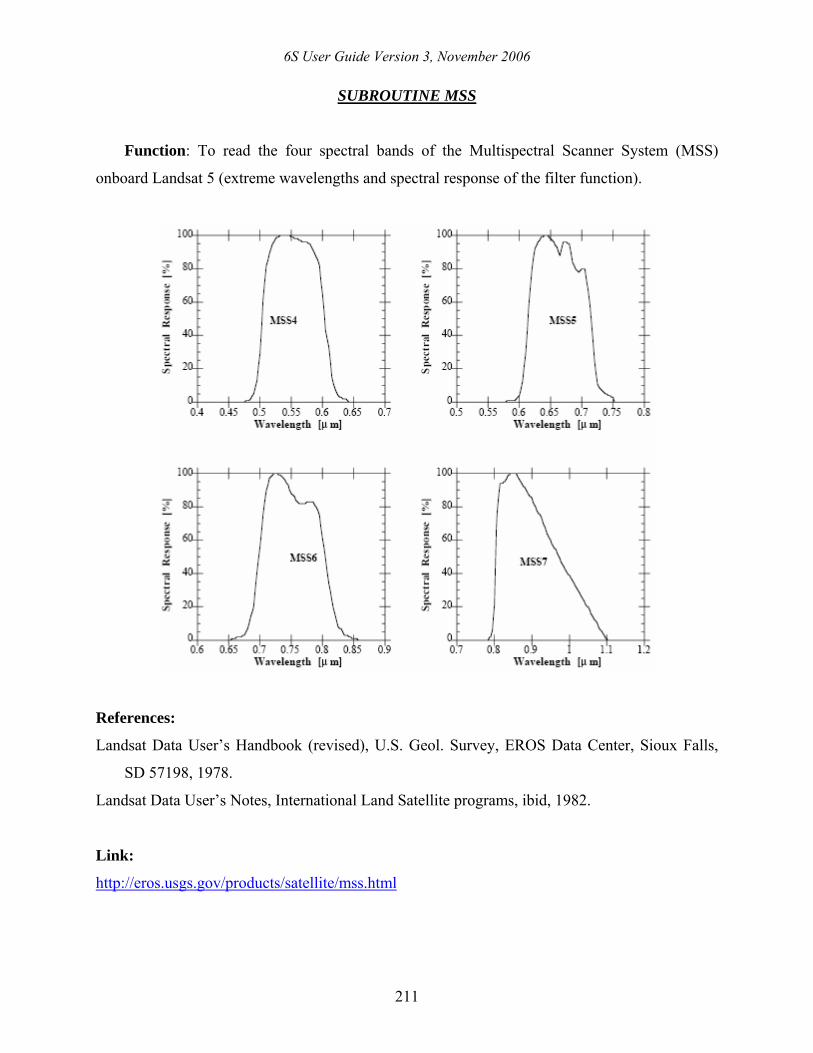
SUBROUTINE MSS
Function: To read the four spectral bands of the Multispectral Scanner System (MSS)
onboard Landsat 5 (extreme wavelengths and spectral response of the filter function).
References:
Landsat Data User’s Handbook (revised), U.S. Geol. Survey, EROS Data Center, Sioux Falls,
SD 57198, 1978.
Landsat Data User’s Notes, International Land Satellite programs, ibid, 1982.
Link:
http://eros.usgs.gov/products/satellite/mss.html
6S User Guide Version 3, November 2006
212
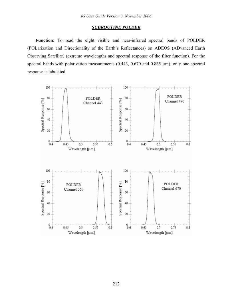
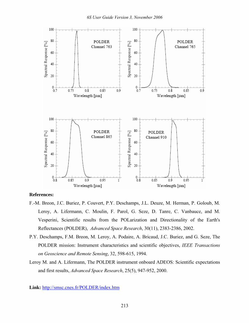
SUBROUTINE POLDER
Function: To read the eight visible and near-infrared spectral bands of POLDER
(POLarization and Directionality of the Earth’s Reflectances) on ADEOS (ADvanced Earth
Observing Satellite) (extreme wavelengths and spectral response of the filter function). For the
spectral bands with polarization measurements (0.443, 0.670 and 0.865 µm), only one spectral
response is tabulated.
6S User Guide Version 3, November 2006
213
References:
F.-M. Breon, J.C. Buriez, P. Couvert, P.Y. Deschamps, J.L. Deuze, M. Herman, P. Goloub, M.
Leroy, A. Lifermann, C. Moulin, F. Parol, G. Seze, D. Tanre, C. Vanbauce, and M.
Vesperini, Scientific results from the POLarization and Directionality of the Earth's
Reflectances (POLDER), Advanced Space Research, 30(11), 2383-2386, 2002.
P.Y. Deschamps, F.M. Breon, M. Leroy, A. Podaire, A. Bricaud, J.C. Buriez, and G. Seze, The
POLDER mission: Instrument characteristics and scientific objectives, IEEE Transactions
on Geoscience and Remote Sensing, 32, 598-615, 1994.
Leroy M. and A. Lifermann, The POLDER instrument onboard ADEOS: Scientific expectations
and first results, Advanced Space Research, 25(5), 947-952, 2000.
Link: http://smsc.cnes.fr/POLDER/index.htm
6S User Guide Version 3, November 2006
214
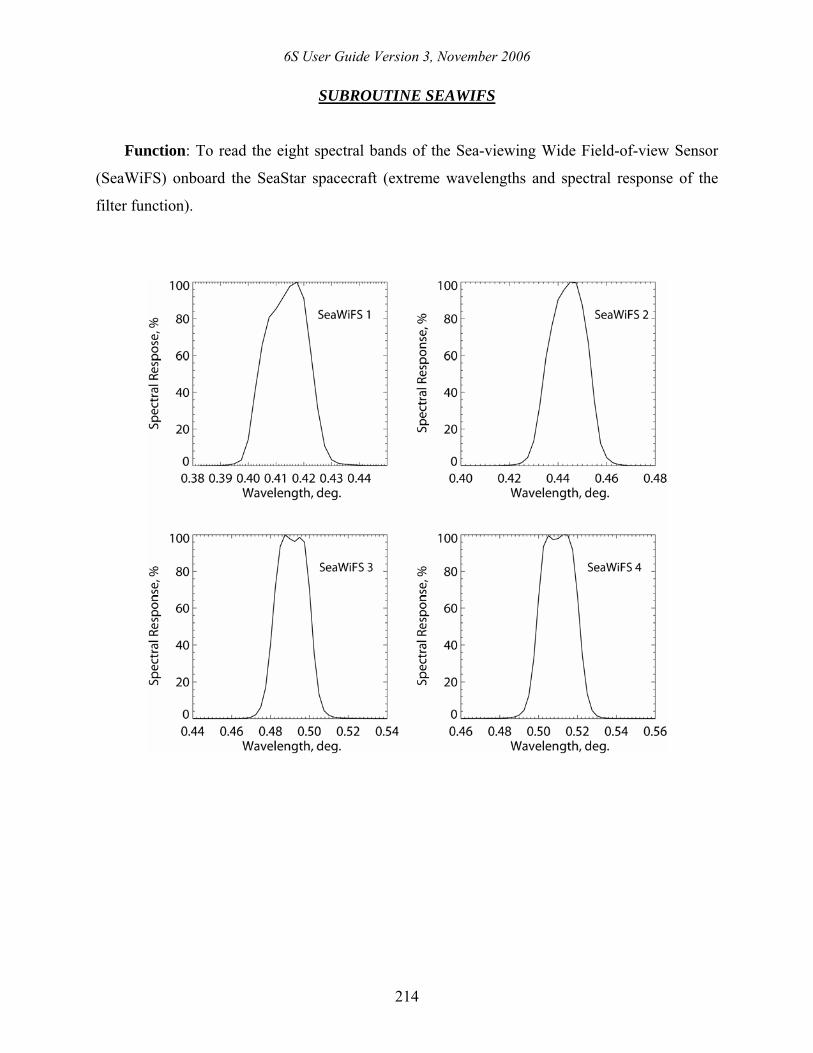
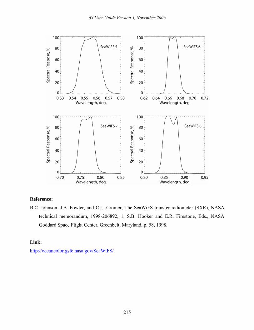
SUBROUTINE SEAWIFS
Function: To read the eight spectral bands of the Sea-viewing Wide Field-of-view Sensor
(SeaWiFS) onboard the SeaStar spacecraft (extreme wavelengths and spectral response of the
filter function).
6S User Guide Version 3, November 2006
215
Reference:
B.C. Johnson, J.B. Fowler, and C.L. Cromer, The SeaWiFS transfer radiometer (SXR), NASA
technical memorandum, 1998-206892, 1, S.B. Hooker and E.R. Firestone, Eds., NASA
Goddard Space Flight Center, Greenbelt, Maryland, p. 58, 1998.
Link:
http://oceancolor.gsfc.nasa.gov/SeaWiFS/
6S User Guide Version 3, November 2006
216
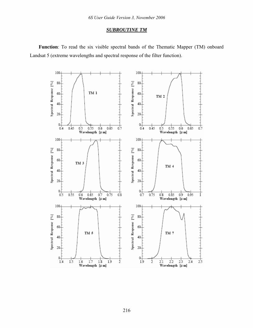
SUBROUTINE TM
Function: To read the six visible spectral bands of the Thematic Mapper (TM) onboard
Landsat 5 (extreme wavelengths and spectral response of the filter function).

6S User Guide Version 3, November 2006
217
Reference:
B.L. Markham and J.L. Barker, Spectral characterization of the LANDSAT Thematic Mapper
sensors, International Journal of Remote Sensing, 6, 697-716, 1985.
Link:
http://eros.usgs.gov/products/satellite/tm.html
6S User Guide Version 3, November 2006
218
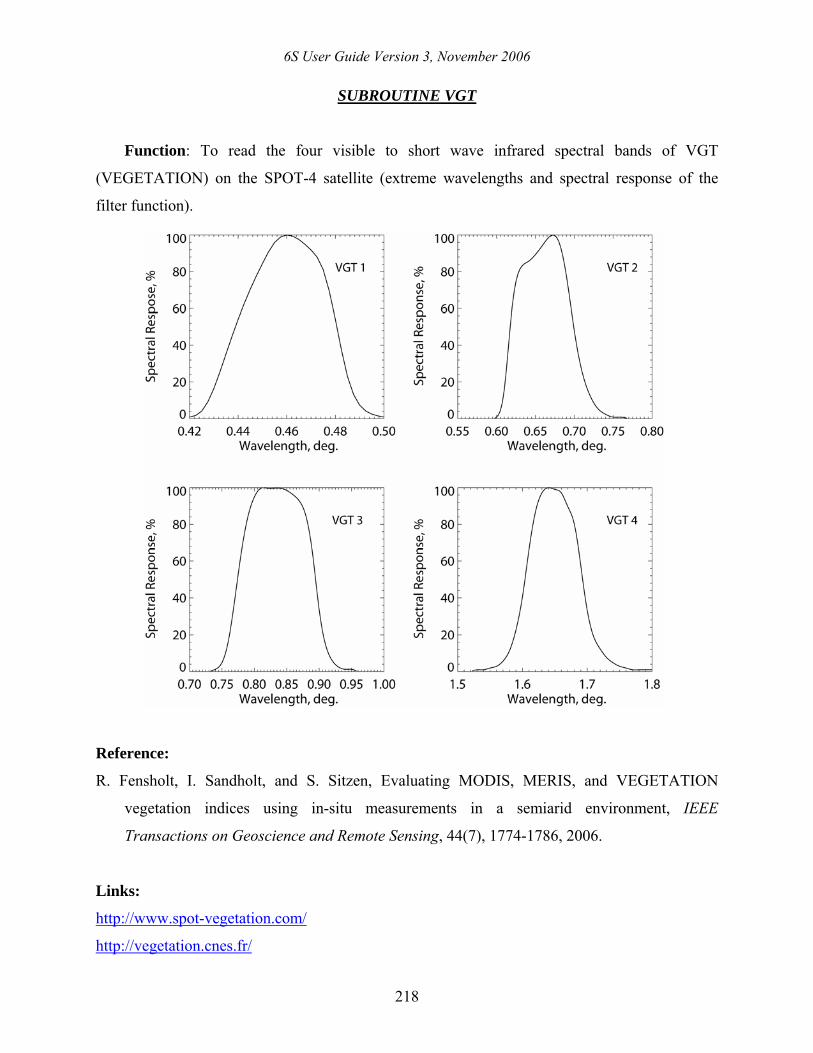
SUBROUTINE VGT
Function: To read the four visible to short wave infrared spectral bands of VGT
(VEGETATION) on the SPOT-4 satellite (extreme wavelengths and spectral response of the
filter function).
Reference:
R. Fensholt, I. Sandholt, and S. Sitzen, Evaluating MODIS, MERIS, and VEGETATION
vegetation indices using in-situ measurements in a semiarid environment, IEEE
Transactions on Geoscience and Remote Sensing, 44(7), 1774-1786, 2006.
Links:
http://www.spot-vegetation.com/
http://vegetation.cnes.fr/
6S User Guide Version 3, November 2006
219
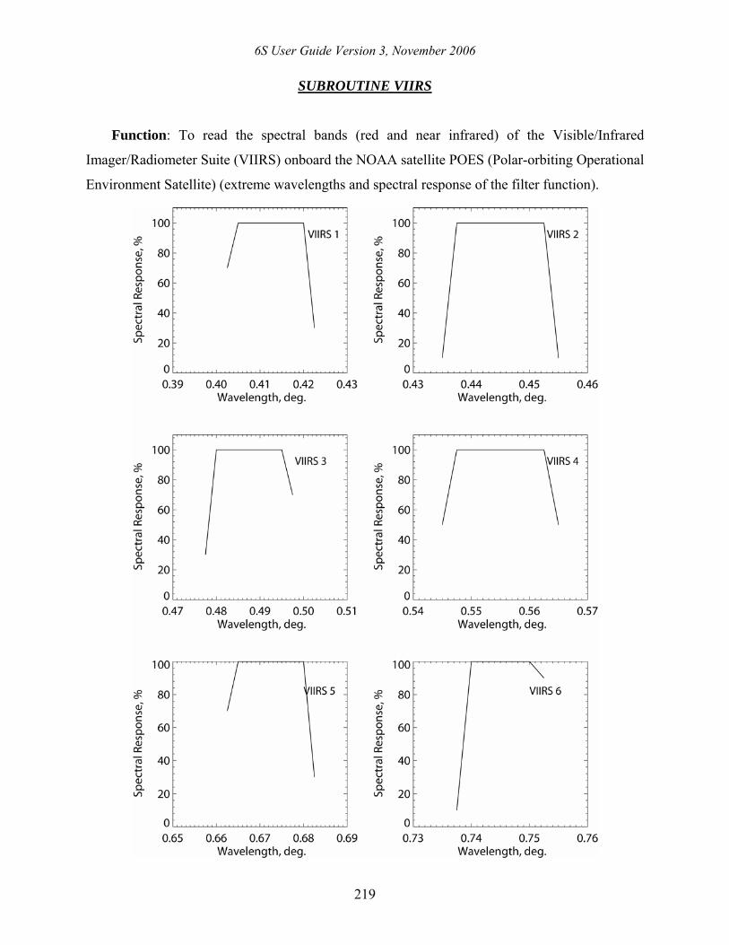
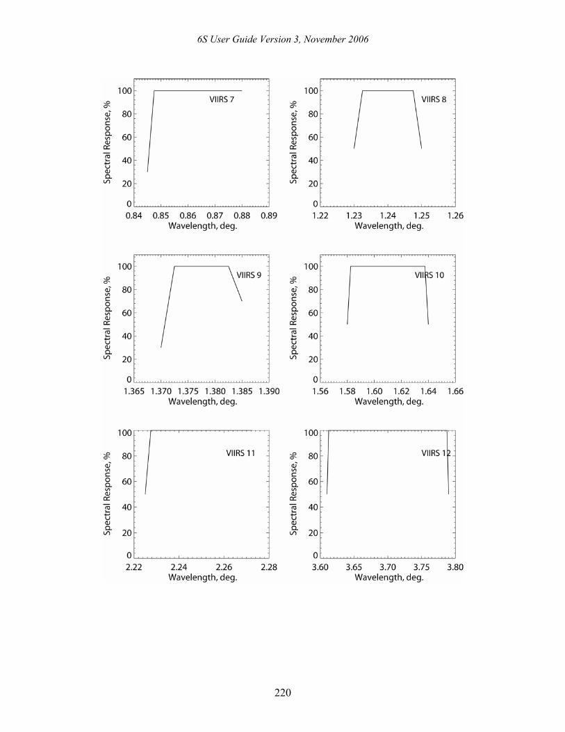
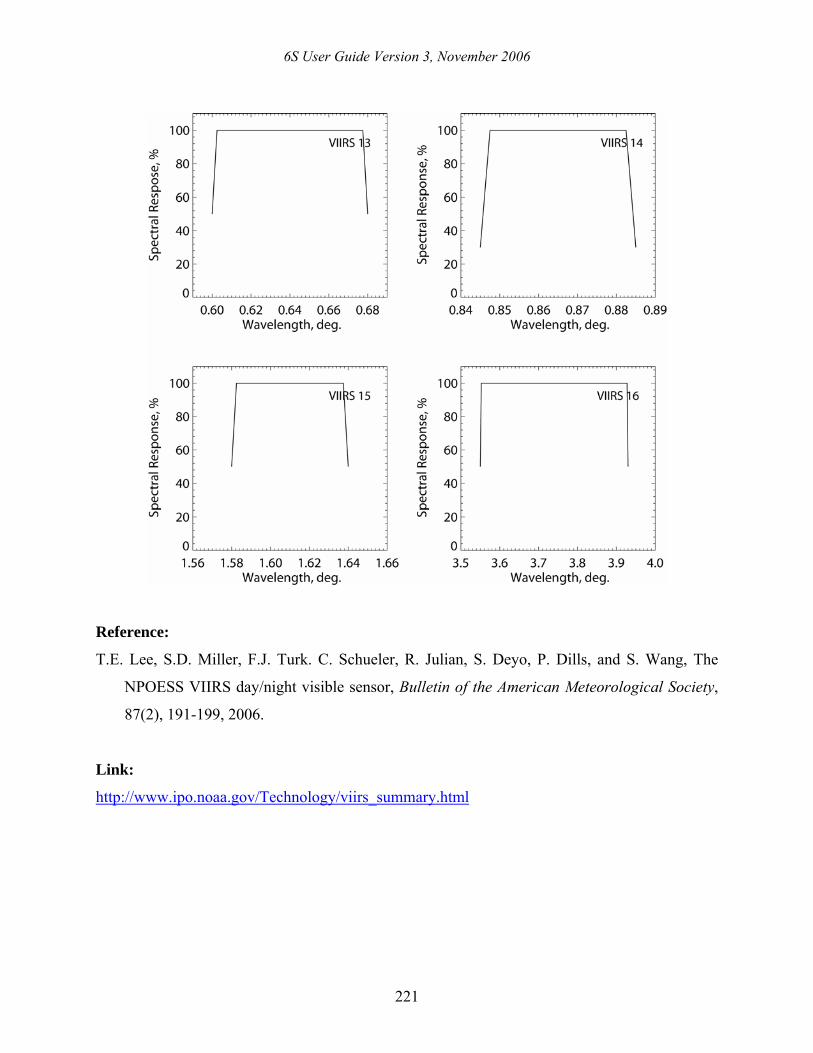
SUBROUTINE VIIRS
Function: To read the spectral bands (red and near infrared) of the Visible/Infrared
Imager/Radiometer Suite (VIIRS) onboard the NOAA satellite POES (Polar-orbiting Operational
Environment Satellite) (extreme wavelengths and spectral response of the filter function).
6S User Guide Version 3, November 2006
220
6S User Guide Version 3, November 2006
221
Reference:
T.E. Lee, S.D. Miller, F.J. Turk. C. Schueler, R. Julian, S. Deyo, P. Dills, and S. Wang, The
NPOESS VIIRS day/night visible sensor, Bulletin of the American Meteorological Society,
87(2), 191-199, 2006.
Link:
http://www.ipo.noaa.gov/Technology/viirs_summary.html
6S User Guide Version 3, November 2006
222
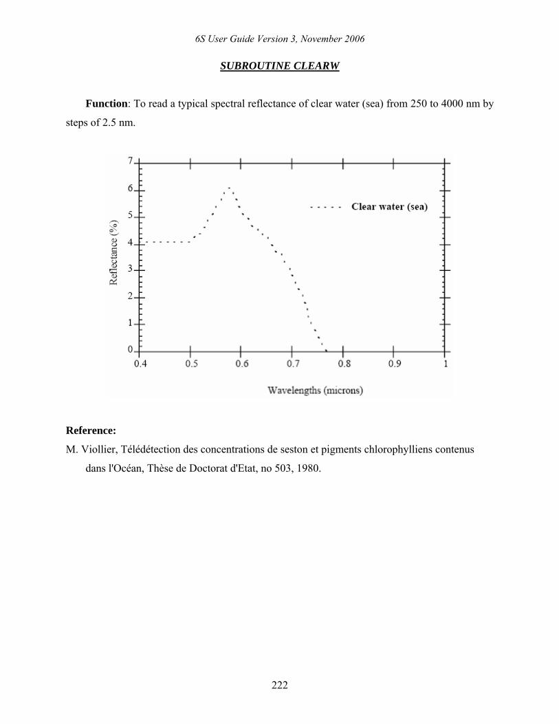
SUBROUTINE CLEARW
Function: To read a typical spectral reflectance of clear water (sea) from 250 to 4000 nm by
steps of 2.5 nm.
Reference:
M. Viollier, Télédétection des concentrations de seston et pigments chlorophylliens contenus
dans l'Océan, Thèse de Doctorat d'Etat, no 503, 1980.
6S User Guide Version 3, November 2006
223
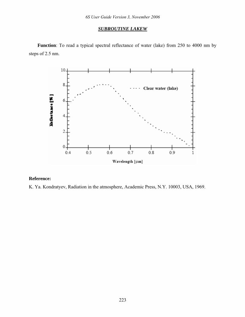
SUBROUTINE LAKEW
Function: To read a typical spectral reflectance of water (lake) from 250 to 4000 nm by
steps of 2.5 nm.
Reference:
K. Ya. Kondratyev, Radiation in the atmosphere, Academic Press, N.Y. 10003, USA, 1969.
6S User Guide Version 3, November 2006
224
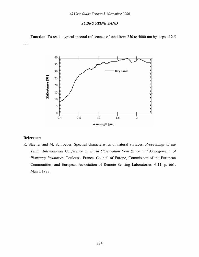
SUBROUTINE SAND
Function: To read a typical spectral reflectance of sand from 250 to 4000 nm by steps of 2.5
nm.
Reference:
R. Staetter and M. Schroeder, Spectral characteristics of natural surfaces, Proceedings of the
Tenth International Conference on Earth Observation from Space and Management of
Planetary Resources, Toulouse, France, Council of Europe, Commission of the European
Communities, and European Association of Remote Sensing Laboratories, 6-11, p. 661,
March 1978.
6S User Guide Version 3, November 2006
225
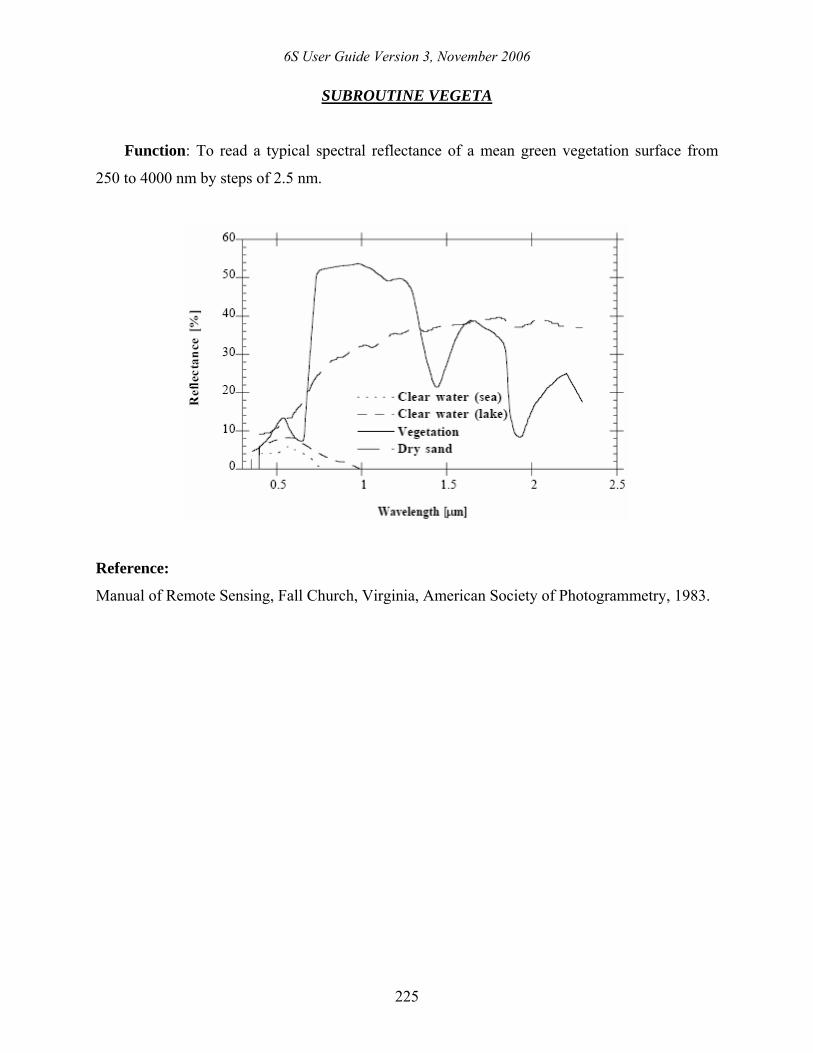
SUBROUTINE VEGETA
Function: To read a typical spectral reflectance of a mean green vegetation surface from
250 to 4000 nm by steps of 2.5 nm.
Reference:
Manual of Remote Sensing, Fall Church, Virginia, American Society of Photogrammetry, 1983.
6S User Guide Version 3, November 2006
226
SUBROUTINE DICA1
Function: To read the eight coefficients necessary to compute the CO2 transmission
according to the Malkmus model (see subroutine ABSTRA). The frequency interval is 2500-
5050 cm-1, step of 10 cm-1.
SUBROUTINE DICA2
Function: Same as DICA1 but for the frequency interval 5060-7610 cm-1.
SUBROUTINE DICA3
Function: Same as DICA1 but for the frequency interval 7620-10170 cm-1.
6S User Guide Version 3, November 2006
227
SUBROUTINE METH1
Function: To read the eight coefficients necessary to compute the methane transmission
according to the Malkmus model (see subroutine ABSTRA). The frequency interval is 2500-
5050 cm-1, step of 10 cm-1.
SUBROUTINE METH2
Function: Same as METH1 but for the frequency interval 5060-7610 cm-1.
SUBROUTINE METH3
Function: Same as METH1 but for the frequency interval 7620-10170 cm-1.
SUBROUTINE METH4
Function: Same as METH1 but for the frequency interval 10180-12730 cm-1.
SUBROUTINE METH5
Function: Same as METH1 but for the frequency interval 12740-15290 cm-1.
SUBROUTINE METH6
Function: Same as METH1 but for the frequency interval 15300-17870 cm-1.
6S User Guide Version 3, November 2006
228
SUBROUTINE MOCA1
Function: To read the eight coefficients necessary to compute the CO transmission
according to the Malkmus model (see subroutine ABSTRA). The frequency interval is 2500-
5050 cm-1, step of 10 cm-1.
SUBROUTINE MOCA2
Function: Same as MOCA1 but for the frequency interval 5060-7610 cm-1
.
SUBROUTINE MOCA3
Function: Same as MOCA1 but for the frequency interval 7620-10170 cm-1
.
SUBROUTINE MOCA4
Function: Same as MOCA1 but for the frequency interval 10180-12730 cm-1
.
SUBROUTINE MOCA5
Function: Same as MOCA1 but for the frequency interval 12740-15290 cm-1
.
SUBROUTINE MOCA6
Function: Same as MOCA1 but for the frequency interval 15300-17870 cm-1
6S User Guide Version 3, November 2006
229
SUBROUTINE NIOX1
Function: To read the eight coefficients necessary to compute the N2O transmission
according to the Malkmus model (see subroutine ABSTRA). The frequency interval is 2500-
5050 cm-1, step of 10 cm-1.
SUBROUTINE NIOX2
Function: Same as NIOX1 but for the frequency interval 5060-7610 cm-1.
SUBROUTINE NIOX3
Function: Same as NIOX1 but for the frequency interval 7620-10170 cm-1.
SUBROUTINE NIOX4
Function: Same as NIOX1 but for the frequency interval 10180-12730 cm-1.
SUBROUTINE NIOX5
Function: Same as NIOX1 but for the frequency interval 12740-15290 cm-1.
SUBROUTINE NIOX6
Function: Same as NIOX1 but for the frequency interval 15300-17870 cm-1.
6S User Guide Version 3, November 2006
230
SUBROUTINE OXYG3
Function: To read the eight coefficients necessary to compute the O2 transmission according
to the Malkmus model (see subroutine ABSTRA). The frequency interval is 2500-5050 cm-1,
step of 10 cm-1.
SUBROUTINE OXYG4
Function: Same as OXYG3 but for the frequency interval 10180-12730 cm-1.
SUBROUTINE OXYG5
Function: Same as OXYG3 but for the frequency interval 12740-15290 cm-1.
SUBROUTINE OXYG6
Function: Same as OXYG3 but for the frequency interval 15300-17870 cm-1.
6S User Guide Version 3, November 2006
231
SUBROUTINE OZON1
Function: To read the eight coefficients necessary to compute the O3 transmission according
to the Malkmus model (see subroutine ABSTRA). The frequency interval is 2500-5050 cm-1,
steps of 10 cm-1.
6S User Guide Version 3, November 2006
232
SUBROUTINE WAVA1
Function: To read the eight coefficients necessary to compute the H2O transmission
according to the Goody model (see subroutine ABSTRA). The frequency interval is 2500-5050
cm-1, steps of 10 cm-1.
SUBROUTINE WAVA2
Function: Same as WAVA1 but for the frequency interval 5060-7610 cm-1.
SUBROUTINE WAVA3
Function: Same as WAVA1 but for the frequency interval 7620-10170 cm-1.
SUBROUTINE WAVA4
Function: Same as WAVA1 but for the frequency interval 10180-12730 cm-1.
SUBROUTINE WAVA5
Function: Same as WAVA1 but for the frequency interval 12740-15290 cm-1.
SUBROUTINE WAVA6
Function: Same as WAVA1 but for the frequency interval 15300-17860 cm-1.
6S User Guide Version 3, November 2006
233
SUBROUTINE DUST
Function: To read the scattering phase function for the dust-like component. Computations
have been performed for 83 angles (80 Gaussian angles and 0°, 90° and 180°) and 20
wavelengths (0.350, 0.400, 0.412, 0.443, 0.470, 0.488, 0.515, 0.550, 0.590, 0.633, 0.670, 0.694,
0.760, 0.860, 1.240, 1.536, 1.650, 1.950, 2.250, and 3.750 nm).
SUBROUTINE OCEA
Function: Same as DUST but for the oceanic component.
SUBROUTINE SOOT
Function: Same as DUST but for the soot component.
SUBROUTINE WATE
Function: Same as DUST but for the water-soluble component.
Reference:
J. Lenoble, ed., Radiative transfer in scattering and absorbing atmospheres: standard
computational procedures, A. DEEPAK Publishing, Hampton, Virginia, USA, 1985.
6S User Guide Version 3, November 2006
234
SUBROUTINE BBM
Function: Same as DUST but for the biomass burning model.
Reference: O. Dubovik, B. Holben, T. F. Eck, A. Smirnov, Y. J. Kaufman, M. D. King, D.
Tanré, and I. Slutsker, Variability of absorption and optical properties of key aerosol types
observed in worldwide locations, Journal of the Atmospheric Sciences, 59, 590-608, 2002.
SUBROUTINE BDM
Function: Same as DUST but for the background desert model.
Reference: G. A. d’Almeida, P. Koepke, and E. P. Shettle, Atmospheric aerosols: global
climatology and radiative characteristics, A. DEEPAK Publishing, Hampton, Virginia, USA,
1991, p. 48, 80 and 120.
SUBROUTINE STM
Function: Same as DUST but for the stratospheric model.
Reference: P.B. Russel, J.M. Livingston, R.F. Pueschel; J.J. Bauman, J.B. Pollac, S.L. Brooks,
P. Hamill, L.W. Thomason, L.L. Stowe, T. Deshler, E.G. Dutton, and R.W. Bergstrom,
Global to microscale evolution of the Pinatubo volcanic aerosol derived from diverse
measurements and analyses, Journal of Geophysical Research, 101(D13), 18745-18763,
1996.
6S User Guide Version 3, November 2006
235
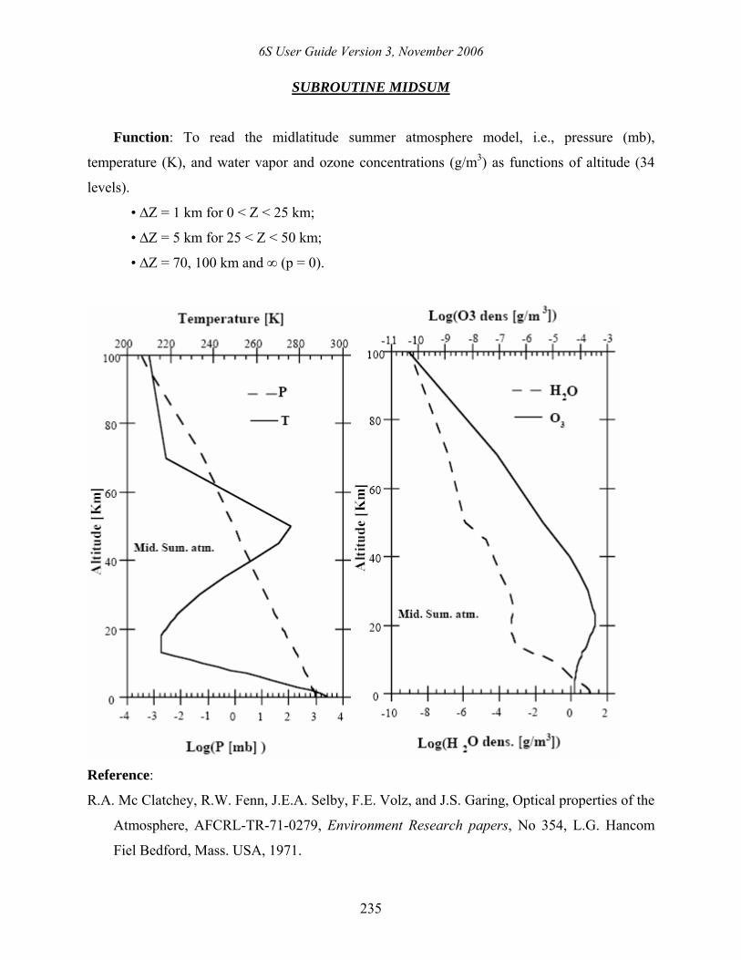
SUBROUTINE MIDSUM
Function: To read the midlatitude summer atmosphere model, i.e., pressure (mb),
temperature (K), and water vapor and ozone concentrations (g/m3) as functions of altitude (34
levels).
• ∆Z = 1 km for 0 < Z < 25 km;
• ∆Z = 5 km for 25 < Z < 50 km;
• ∆Z = 70, 100 km and ∞ (p = 0).
Reference:
R.A. Mc Clatchey, R.W. Fenn, J.E.A. Selby, F.E. Volz, and J.S. Garing, Optical properties of the
Atmosphere, AFCRL-TR-71-0279, Environment Research papers, No 354, L.G. Hancom
Fiel Bedford, Mass. USA, 1971.
6S User Guide Version 3, November 2006
236
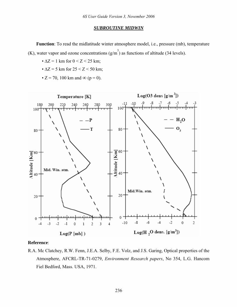
SUBROUTINE MIDWIN
Function: To read the midlatitude winter atmosphere model, i.e., pressure (mb), temperature
(K), water vapor and ozone concentrations (g/m3) as functions of altitude (34 levels).
• ∆Z = 1 km for 0 < Z < 25 km;
• ∆Z = 5 km for 25 < Z < 50 km;
• Z = 70, 100 km and ∞ (p = 0).
Reference:
R.A. Mc Clatchey, R.W. Fenn, J.E.A. Selby, F.E. Volz, and J.S. Garing, Optical properties of the
Atmosphere, AFCRL-TR-71-0279, Environment Research papers, No 354, L.G. Hancom
Fiel Bedford, Mass. USA, 1971.
6S User Guide Version 3, November 2006
237
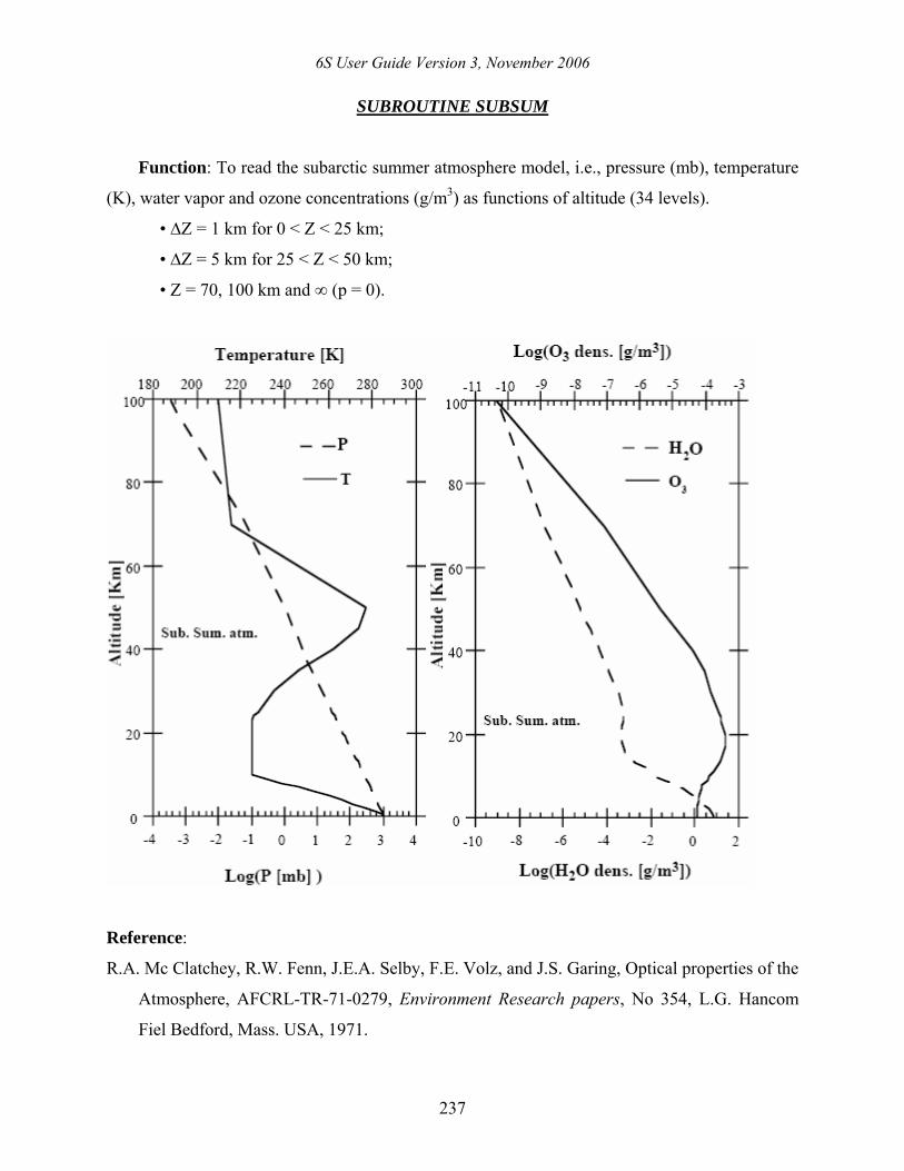
SUBROUTINE SUBSUM
Function: To read the subarctic summer atmosphere model, i.e., pressure (mb), temperature
(K), water vapor and ozone concentrations (g/m3) as functions of altitude (34 levels).
• ∆Z = 1 km for 0 < Z < 25 km;
• ∆Z = 5 km for 25 < Z < 50 km;
• Z = 70, 100 km and ∞ (p = 0).
Reference:
R.A. Mc Clatchey, R.W. Fenn, J.E.A. Selby, F.E. Volz, and J.S. Garing, Optical properties of the
Atmosphere, AFCRL-TR-71-0279, Environment Research papers, No 354, L.G. Hancom
Fiel Bedford, Mass. USA, 1971.
6S User Guide Version 3, November 2006
238
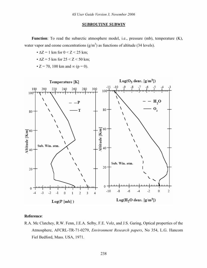
SUBROUTINE SUBWIN
Function: To read the subarctic atmosphere model, i.e., pressure (mb), temperature (K),
water vapor and ozone concentrations (g/m3) as functions of altitude (34 levels).
• ∆Z = 1 km for 0 < Z < 25 km;
• ∆Z = 5 km for 25 < Z < 50 km;
• Z = 70, 100 km and ∞ (p = 0).
Reference:
R.A. Mc Clatchey, R.W. Fenn, J.E.A. Selby, F.E. Volz, and J.S. Garing, Optical properties of the
Atmosphere, AFCRL-TR-71-0279, Environment Research papers, No 354, L.G. Hancom
Fiel Bedford, Mass. USA, 1971.
6S User Guide Version 3, November 2006
239
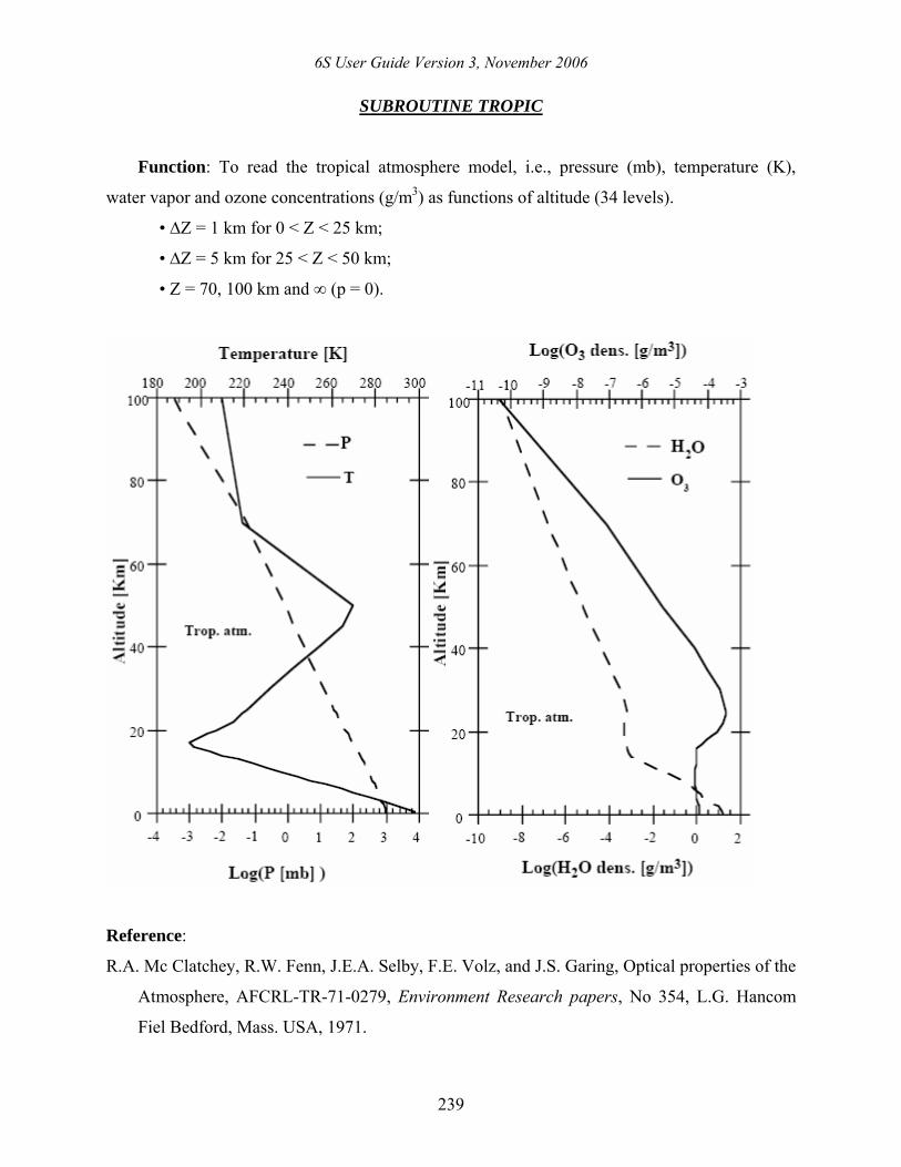
SUBROUTINE TROPIC
Function: To read the tropical atmosphere model, i.e., pressure (mb), temperature (K),
water vapor and ozone concentrations (g/m3) as functions of altitude (34 levels).
• ∆Z = 1 km for 0 < Z < 25 km;
• ∆Z = 5 km for 25 < Z < 50 km;
• Z = 70, 100 km and ∞ (p = 0).
Reference:
R.A. Mc Clatchey, R.W. Fenn, J.E.A. Selby, F.E. Volz, and J.S. Garing, Optical properties of the
Atmosphere, AFCRL-TR-71-0279, Environment Research papers, No 354, L.G. Hancom
Fiel Bedford, Mass. USA, 1971.
6S User Guide Version 3, November 2006
240
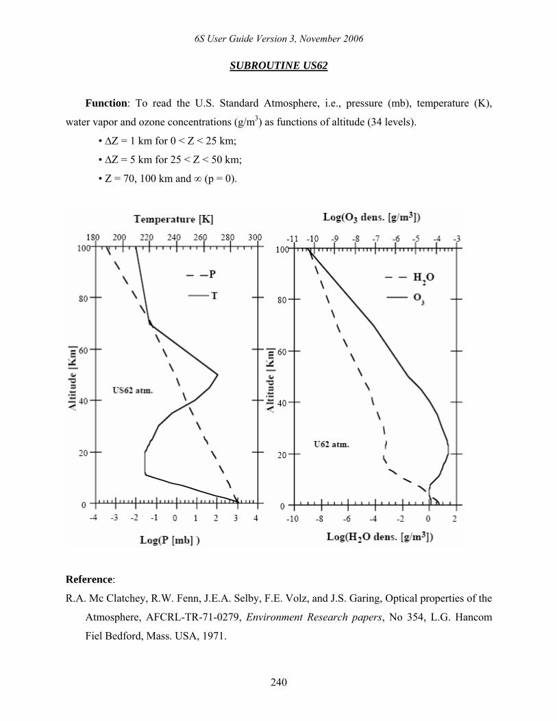
SUBROUTINE US62
Function: To read the U.S. Standard Atmosphere, i.e., pressure (mb), temperature (K),
water vapor and ozone concentrations (g/m3) as functions of altitude (34 levels).
• ∆Z = 1 km for 0 < Z < 25 km;
• ∆Z = 5 km for 25 < Z < 50 km;
• Z = 70, 100 km and ∞ (p = 0).
Reference:
R.A. Mc Clatchey, R.W. Fenn, J.E.A. Selby, F.E. Volz, and J.S. Garing, Optical properties of the
Atmosphere, AFCRL-TR-71-0279, Environment Research papers, No 354, L.G. Hancom
Fiel Bedford, Mass. USA, 1971.

6S User Guide Version 3, November 2006
241
MISCELLANEOUS

6S User Guide Version 3, November 2006
242
SUBROUTINE EQUIVWL
Function: To compute the equivalent wavelength needed for the calculation of the
downward radiation field used in the computation of the non-Lambertian target contribution (file
main.f).
Description: The input is the spectral response of the selected sensor as well as the solar
irradiance spectrum. The output is the equivalent wavelength which is computed by averaging
the spectral response of the sensor over the solar irradiance using an increment of 2.5 nm.
SUBROUTINE PRINT_ERROR
Function: To provide centralized error handling for the code and specific output error
messages.
6S User Guide Version 3, November 2006
243
SUBROUTINE SPECINTERP
Function: To compute atmospheric properties at the equivalent wavelength (see subroutine
EQUIVWL) needed for the calculation of the downward radiation field used in the computation
of the non-Lambertian target contribution (file main.f).
Description: The input is the equivalent wavelength for which the coupling between the
BRDF and the atmosphere is to be computed. Using the actual aerosol model, the outputs are the
atmospheric properties at this wavelength, that is the aerosol optical thickness, single scattering
albedo and phase function. In addition, this routine modifies the thickness and single scattering
albedo of the aerosol layer below an aircraft.
SUBROUTINE SPlIE2, SPLIN2, SPLINE, SPLINT
Function: To perform interpolation of a furnished BDRF discrete dataset (BRDFGRID,
option 1 of the BRDF model) to compute the albedo and BRDF value at the Gaussian quadrature
points.