
C LMN MODEL TO COMPUTE BEST ESTIMATES IN … model calibration - 1 - CALIBRATING LMN MODEL TO...
30
LMN model calibration - 1 - CALIBRATING LMN MODEL TO COMPUTE BEST ESTIMATES IN LIFE INSURANCE Version 1.2 of 08/04/2015 Yacine Laïdi Ψ Frédéric Planchet * ISFA - Laboratoire SAF β Université de Lyon - Université Claude Bernard Lyon 1 ABSTRACT In this paper, we propose to study a method for calibrating Longstaff, Mithal and Neis model (or LMN model) from a CDS (credit derivative swaps) and bonds associated with the same entity as the CDS. This model is used by many insurers. The calculations will use at each observation date a risk-free rate curve generated through Nelson, Siegel and Svensson method from swap rates vs. six-month Euribor. The process will decompose the spread attributed to the reference entity and will especially evaluate the component associated to default risk and the one associated to liquidity risk. The entity will be Deutsch Bank AG. The study will reveal the existence of a negative liquidity component for some corporate bonds and at some cotation dates, which will show that rate swaps indexed on six- month Euribor include an implied spread. Calibration data come from cotations provided by Reuters and the studied period spreads from the 5th January 2009 to the 30th December 2011. The main idea of this paper is that parameters must be determined to ensure the prices from the model represent the best possible prices observed not at a given date, but over a fixed period. The practical implementation of this idea requires the use of a genetic algorithm, which we present here. Ψ Yacine Laïdi is an IT consultant at Smart Trade Services and an associate actuary. Contact: [email protected]. * Frédéric Planchet is professor at ISFA and partner actuary at Prim’Act. Contact: [email protected]. β Institut de Science Financière et d’Assurances (ISFA) - 50 avenue Tony Garnier - 69366 Lyon Cedex 07 - France.
Transcript of C LMN MODEL TO COMPUTE BEST ESTIMATES IN … model calibration - 1 - CALIBRATING LMN MODEL TO...
LMN model calibration - 1 -
CALIBRATING LMN MODEL TO COMPUTE BEST ESTIMATES IN LIFE
INSURANCE
Version 1.2 of 08/04/2015
Yacine LaïdiΨ Frédéric Planchet∗
ISFA - Laboratoire SAF β
Université de Lyon - Université Claude Bernard Lyon 1
ABSTRACT
In this paper, we propose to study a method for calibrating Longstaff, Mithal and Neis model (or LMN model) from a
CDS (credit derivative swaps) and bonds associated with the same entity as the CDS. This model is used by many
insurers. The calculations will use at each observation date a risk-free rate curve generated through Nelson, Siegel and
Svensson method from swap rates vs. six-month Euribor. The process will decompose the spread attributed to the
reference entity and will especially evaluate the component associated to default risk and the one associated to
liquidity risk. The entity will be Deutsch Bank AG. The study will reveal the existence of a negative liquidity
component for some corporate bonds and at some cotation dates, which will show that rate swaps indexed on six-
month Euribor include an implied spread.
Calibration data come from cotations provided by Reuters and the studied period spreads from the 5th January 2009 to
the 30th December 2011.
The main idea of this paper is that parameters must be determined to ensure the prices from the model represent the
best possible prices observed not at a given date, but over a fixed period. The practical implementation of this idea
requires the use of a genetic algorithm, which we present here.
Ψ Yacine Laïdi is an IT consultant at Smart Trade Services and an associate actuary. Contact: [email protected]. ∗ Frédéric Planchet is professor at ISFA and partner actuary at Prim’Act. Contact: [email protected]. β Institut de Science Financière et d’Assurances (ISFA) - 50 avenue Tony Garnier - 69366 Lyon Cedex 07 - France.
LMN model calibration - 2 -
AGENDA
1. Introduction ......................................................................................................................... 2
2. Model description ................................................................................................................ 4 3. Calibrating LMN model ...................................................................................................... 9
3.1. Choosing and collecting data ................................................................................... 10 3.2. Data description ........................................................................................................ 13 3.3. Principle of calibration algorithm............................................................................. 14
3.3.1. Computing model parameters .............................................................................. 15
3.3.2. Measuring the spread components of a corporate bond ....................................... 18
3.3.3. Alternative method ............................................................................................... 20 4. Analysing the results ......................................................................................................... 21
4.1. Fitting quality ........................................................................................................... 21 4.2. Decomposing the yield to maturity of a bond .......................................................... 22
4.3. Out of sample test ..................................................................................................... 23 5. Conclusion ......................................................................................................................... 25
6. References ......................................................................................................................... 26
7. Appendix ........................................................................................................................... 27
7.1. Fitting quality ........................................................................................................... 28 7.2. Decomposing the yield to maturity of a bond .......................................................... 29
7.3. Out of sample test ..................................................................................................... 29
1. INTRODUCTION
In the last ten years, we have observed a generalization of the use of “economic valuations” in
various frameworks used by insurers: regulation (Solvency II), accounting (IFRS) and financial
reporting (MCEV). This led to the use by insurers of methods originally developed for pricing
financial instruments to calculate their liabilities. On this occasion, many challenges have
emerged, particularly in life insurance, e.g. long duration of life insurance liabilities, no market for
insurance liabilities, partially endogenous risk factors and volatility of the value which does not
reflect the risks carried.
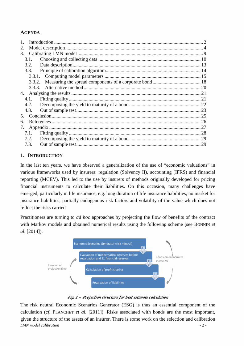
Practitioners are turning to ad hoc approaches by projecting the flow of benefits of the contract
with Markov models and obtained numerical results using the following scheme (see BONNIN et
al. [2014]):
Economic Scenarios Generator (risk neutral)
Evaluation of mathematical reserves before
revaluation and S1 financial reserves
Calculation of profit sharing
Revaluation of liabilities
Iteration of projection time
Loops on economicalscenarios
Fig. 1 – Projection structure for best estimate calculation
The risk neutral Economic Scenarios Generator (ESG) is thus an essential component of the
calculation (cf. PLANCHET et al. [2011]). Risks associated with bonds are the most important,
given the structure of the assets of an insurer. There is some work on the selection and calibration

LMN model calibration - 3 -
of models for the risk-free interest rate (see e.g. MOUDIKI [2014] and the references therein). But
corporate bond yield offers a spread on risk-free rate, composed of default risk rate and a residual
spread which can be interpreted as a liquidity indicator. Default risk component of a bond can be
extracted from data on CDS premiums. There is however very little work those risks in this very
specific context.
To model this spread risk in order to compute savings contract best estimates, LMN model
elaborated by LONGSTAFF et al. [2005] represents an attractive choice in that it is easy to
implement and allows to take efficiently this risk into account. It is therefore often chosen by
insurers (see OUAJJOU [2010]). It is also the chosen model in ESG package1.
The reasons of this choice are the following ones:
� The existence of analytical forms to compute the price of a corporate zero coupon
bond, which makes the implementation easier due to the existence of closed forms to
compute zero coupon price.
� Its compatibility with all risk-free rate models. Deduced forms do not depend on the
choice of a particular risk-free rate model.
However, if this model turns out to be simple to use, its calibration is difficult. The aim of this
paper is to propose a calibration method adapted to insurance context.
More precisely, it is necessary to define a coherent model calibration with both the observed
prices and the long-term horizon. Calibration should be relatively stable when updated on nearby
dates. The purpose of this paper is to propose a method for a consistent estimation of the
parameters of the LMN model that respects this constraint. A method using only the last known
prices, as in LONGSTAFF et al. [2005] is obviously not relevant here, because it actually induces
volatility of the parameters that is not representative of the risks actually incurred. The stochastic
processes used for risk factors have constant coefficients and the choice of the parameters must be
consistent with this hypothesis over a short period.
We can see that price volatility and therefore the associated calibration is a matter of concern to
the regulator. The latest specifications of the standard formula provide a volatility adjustment (see
EIOPA [2014]) whose objective is to stabilize the calculation results (that is to say reserves and net
asset value). But this adjustment assumes that volatility is the result of the volatility of the single
liquidity premium. Our approach does not make this assumption and is therefore complementary
to the proposal of the regulator.
The main idea of this paper is that parameters must be determined to ensure the prices from the
model represent the best possible prices observed not at a given date, but over a fixed period. The
practical implementation of this idea requires the use of a genetic algorithm, which we present
here.
1 http://cran.r-project.org/web/packages/ESG/index.html

LMN model calibration - 4 -
2. MODEL DESCRIPTION
Like other reduced-form models LMN model does not directly explain default cause. It rather
focus on modelling corporate default probability and this default can occur at any time. The figure
Fig. 2 describes how this algorithm calculates corporate bond payment flow at a date of coupon
detachment. Let:
� ( )0V t , the flow value at date0t ,
� C , the coupon value,
� c , the coupon value in percentage,
� M , the nominal amount,
� 1, , Nt t… , the dates of future coupon payments,
� 1, ,Mt t− −… , the dates of past coupon payments,
� δ , the time interval between two consecutive coupon payments, this time interval
being assumed constant,
� 0t , the current date.
� Nt , the bond maturity date.
We can write: C cM= et ( )1M C M c+ = + . It follows:
( ) [ ] ( )[ ] ( )
0 00
0
If no default occurs
1 Otherwise
P t F tV t
P t M
ττ ω
> ×= ≤ × − ×
and
( ) 00
0
If
If N
N
C t tF t
C M t t
<= + =
Furthermore, we suppose that payment occurs at default moment, which is not necessarily true in
practice.

LMN model calibration - 5 -
Fig. 2 – Flows of a corporate bond
We note:
� rτ , the risk-free rate, � τλ , the intensity of the Poisson process governing default, � τγ , a convenience yield or liquidity process, which will be used to catch the additional
return investors may require, in addition to compensating credit risk, from holding a corporate bond rather than a riskless bond with similar characteristics.
� ω , the recovery rate.
The three process are stochastic and supposed to be decorrelated from each other. The recovery
rate is arbitrarily fixed at 50 %. LONGSTAFF et al. [2005] assume that those simplifications have
little effect on empirical results. The recovery rate of a corporate bond can be formulated as:
t t t trc r λ γ= + + (1)
There is no need to specify risk-neutral dynamics of risk-free rate to solve for CDS premiums and
corporate bond prices. We only need that these dynamics be such that the price of a risk-free zero-
coupon bond ( )0,P T with maturityT be written as:
( ) ( )00, exp
TP T E r dτ τ = −
∫ (2)
The risk-neutral dynamics of the intensity process (of CIR type) is given by:
( )d d dZττ τ τ λλ α βλ τ σ λ= − + (3)
Whereα , β etσ are positive constants andZτλ a standard Brownian motion. These dynamics allow
for both mean reversion and conditional heteroskedasticity in corporate spreads, and ensure that

LMN model calibration - 6 -
default intensity keeps positive or zero. The liquidity process follows a risk-neutral dynamics
expressed as:
d dZγγ η= (4)
Whereη is a positive constant andZγ also a standard Brownian motion. These dynamics allow the
liquidity process to take positive and negative values. Following DUFFIE [1998], LANDO [1998]
and DUFFIE et al. [1999], it is natural to represent the value of a corporate bond and the values of
premium and protection legs of a CDS as simple expectations under the risk-neutral probability.
For simplification purpose, we assume that the couponc is continuously paid as long as no default
occurs. The price of a corporate bond with maturityT can be simply expressed as a combination of
the different involved process (see LONGSTAFF et al. [2005] whose we will use most closed forms
required to calibration realized in this work).
Bond price is given by:
( ) ( ) ( )( ) ( ) ( )( ) ( )( ) ( ) ( )
( ) ( )( ) ( ) ( ) ( ) ( )( )
0
0
, , exp 0,
exp 0,
1 exp 0,
T
T
T
CB c T c A B C P e d
A T B T C T P T e
B C P G H e d
γτ
γ
γτ
ω τ τ λ τ τ τ
λ
ω τ λ τ τ τ τ λ τ
−
−
−
=
+
+ − +
∫
∫
(5)
and premium CDS is given by:
( )( ) ( ) ( ) ( )( )( ) ( )( ) ( )
0
0
exp 0,
exp 0,
T
T
B P G H ds
A B P d
ω τ λ τ τ τ λ τ
τ τ λ τ τ
+= ∫
∫ (6)
where:
( ) ( )
( ) ( )( )
( ) ( ) ( )
( ) ( )
2
2
2
2
2
2 2
2 3
21
2
222
2
2 2
1exp
1
2
1
exp6
11 exp
1
1exp
1
2
t
Ae
Be
tC
G t ee
He
ασ
φτ
φ
ασφτ
φτ
ασ
φτ
α β φ κτ τσ κ
β φ φτσ σ κ
ητ
α β φα κτφ σ κ
α β φ φσ κτ τσ κ
φ σ ββ φκβ φ
+
+
+ − = −
− = + − = + − = − −
+ + − = −
= ++=−
(7)
We can note that, if 0λ = , then 0s = , which is consistent with the fact that default cost must be
zero, if entity bears no default risk.

LMN model calibration - 7 -
Regarding the pricing of a CDS, it is important to remember that swaps are contracts, not
securities. Therefore, due to their contractual nature, they are less sensitive to liquidity and
convenience yield effects:
- Securities are in fixed supply. By contrast, the notional amount of a CDS may be
arbitrarily high, which implies that laws of supply and demand likely to affect
corporate bonds are much less likely to affect CDS.
- Generic or fungible nature of payment flows prevent CDS from becoming “special” in
a similar way to sovereign bonds or popular stocks on market.
- Since new CDS can always be created, these contracts are much less prone to be
“compressed” than the underlying corporate bonds.
- Since CDS look like insurance contracts, a lot of investors purchasing credit protection
may intend to do so for a fixed horizon and, consequently, may not intend to close out
their position earlier.
- Even though an investor plans to unwind a CDS position, it may be less costly for him
to simply enter into a new CDS in the opposite direction than to attempt to unwind his
current position. Subsequently, the liquidity of his current position is less relevant due
to his capacity to duplicate swap cash flows via other contracts.
- It can sometimes be hard and onerous to sell corporate bonds. However, it is normally
easier to sell a protection than buy one on CDS market.
- At last, BLANCO et al. [2004] notice that credit derivative markets are more liquid that
corporate bond markets in the meaning that new information is captured more quickly
by CDS premiums than by corporate bond prices.
We suppose here that the convenience yield or illiquidity processτγ can be applied to the cash
flows generated by corporate bonds, but not to the cash flows generated by CDS contracts.
Alternatively, τγ can be considered as the differential convenient yield between corporate securities
and credit derivative contracts. Thus, if CDS contracts embed a liquidity component, thenτγ may
underestimate spread component non relative to corporate default. We denote:
� s, the premium paid by the protection buyer against default. � δ ′ , the premium payment frequency. � ( )1M
t ′− + , the CDS starting date.
� Nt ′ , the CDS maturity date.
� 0t , the default date of the reference entity.
� 1, , Nt t ′… , the dates of future premium payments.
� 1, ,Mt t′− −… , the dates of past premium payments.
The figure Fig. 3 describes the generated cash flows if some default occurs before the maturity of
the contract.

LMN model calibration - 8 -
Fig. 3 – Cash flows generated by a CDS when default occurred
Given the dynamics of the intensity and liquidity process, standard results obtained by DUFFIE et
al. [1999] allow for easily inferring closed forms respectively for corporate bond price and for
CDS premium. These forms are also used by LONGSTAFF et al. [2005] and we refer the reader to
them. Let’s examine now some strip bond and some CDS. We note:
� ( )réely , the real bond yield.
� ( )réelr , the riskless component of the total yield. � ( )réel
defs , the default component of the total yield.
� ( )réelliqs , the liquidity component of the total yield.
� CDSs , the CDS premium. � b , the bias or the difference between the sum of the riskless rate and the default
component, and the CDS premium.
The bias b comes from using CDS premium to estimate bond spread default component.
LONGSTAFF et al. [2005] show that CDS premium is a downward biased estimation of the default
component of bond yield in stability period, but it becomes an upward biased estimation when
reference entity gets close to bankruptcy.
The figure Fig. 4 shows the relationships between the above values.
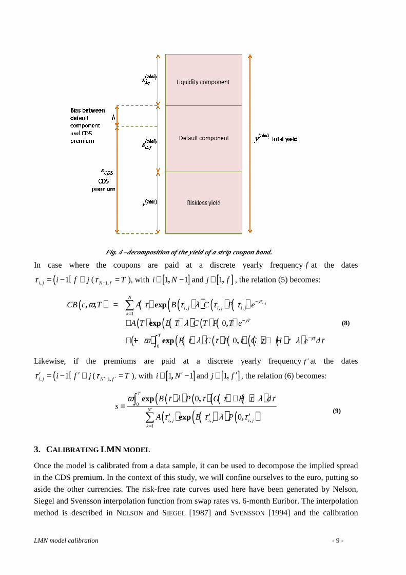
LMN model calibration - 9 -
Fig. 4 –decomposition of the yield of a strip coupon bond.
In case where the coupons are paid at a discrete yearly frequencyf at the dates
( )1,i j i f jτ = − + ( 1,N f Tτ − = ), with [ ]1 1,i N∈ − and [ ]1,j f∈ , the relation (5) becomes:
( ) ( ) ( )( ) ( ) ( )( ) ( )( ) ( ) ( )
( ) ( )( ) ( ) ( ) ( ) ( )( )
1
0
0
1 0
,
, , ,, , exp
exp ,
exp ,
i j
N
i i j i j i jk
T
T
CB c T A B C P e
A T B T C T P T e
B C P G H e d
γτ
γ
γτ
ω τ τ λ τ τ
λ
ω τ λ τ τ τ τ λ τ
−
=−
−
=
+
+ − +
∑
∫
(8)
Likewise, if the premiums are paid at a discrete yearly frequencyf ′ at the dates
( )1,i j i f jτ ′ ′= − + ( 1,N f Tτ ′ ′− = ), with [ ]1 1,i N ′∈ − and [ ]1,j f ′∈ , the relation (6) becomes:
( )( ) ( ) ( ) ( )( )
( ) ( )( ) ( )0
1
0
0, , ,
exp ,
exp ,
T
N
i j i j i jk
B P G H ds
A B P
ω τ λ τ τ τ λ τ
τ τ λ τ′
=
+=
′ ′ ′
∫
∑
(9)
3. CALIBRATING LMN MODEL
Once the model is calibrated from a data sample, it can be used to decompose the implied spread
in the CDS premium. In the context of this study, we will confine ourselves to the euro, putting so
aside the other currencies. The risk-free rate curves used here have been generated by Nelson,
Siegel and Svensson interpolation function from swap rates vs. 6-month Euribor. The interpolation
method is described in NELSON and SIEGEL [1987] and SVENSSON [1994] and the calibration

LMN model calibration - 10 -
process is explained in GILLI et al. [2010]. Besides, the different calibration functions are
optimized through a differential evolution algorithm described in STORN and PRICE [1997].
3.1. CHOOSING AND COLLECTING DATA
The first considered approach consists of computing a CDS premium from a sample bearing
market’s and our portfolio’s features. Nevertheless, given the difficulty to find appropriate data for
such a method and to take into account the correlations between the different entities, this
approach was dropped.
Next, we studied an approach mainly based on bond and CDS indexes. The advantage of an index
is to synthesize the evolution of a market or an asset family, to be usable as a standard measure of
managers’ performance and to serve as an underlying basis for different derivatives.
Bond index families published by Markit Group2 (Markit Credit Indices) caught our attention:
− The Markit iBoxx EUR High Yield index family. This family tracks the performance of euro-denominated sub-investment grade corporate debt and aims to provide appropriate reference portfolios. In addition to a global index, index values are broken down according to maturity, rating and sector. The iBoxx EUR Core High Yield indices includes the standard bond structures are included. An exhaustive framework is built both at bond and index levels, including yield, duration, convexity, fixed-to-floater bonds, excess returns, spreads, etc. This family includes bonds with the following characteristics:
o Fixed coupon bonds (“plain vanilla” bonds), o Zero coupon bonds, o Floating rate notes with EURIBOR as a reference interest rate without cap or floor, o Sinking funds with known redemption schedules, o Bonds with American and European call options, o Bonds with poison put options, o Bonds with make-whole call or tax changes call provisions, o Event-driven bonds such as rating and registration-sensitive bonds, o Payment-in-kind bonds, o Callable perpetuals, o Callable Fixed-to-floater bonds.
− The iBoxx EUR Benchmark index family. This index family is published by the International
Index Company Limited (IIC) and represents the investment grade fixed-income market for Euro denominated bond. It includes an overall index and four subfamilies of main indexes. The sovereign index subfamily is composed of sovereign debts issued by a government from euro zone and denominated in euro or in a former currency from euro zone. This subfamily include an overall and maturity indexes. An overall index is published for each euro zone country (excepted Luxembourg), namely Austria, Belgium, Finland, France, Germany, Greece, Ireland, Italy, the Netherlands, Portugal and Spain. The sovereign index subfamily is complemented by maturity indexes for Germany, France and Italy. The iBoxx EUR Non-Sovereigns index include all bonds which do not meet the iBoxx EUR Sovereigns index’s criteria. Those bonds are next classified into index sub-groups of sub-sovereign, collateralized and corporate bonds. The iBoxx EUR Other Sovereigns index
2 http://www.markit.com/en/

LMN model calibration - 11 -
comprises sovereign bonds issued by countries outside euro zone within sub-sovereign index subgroup. Corporate bond indexes include an overall index and indexes by rating and maturity, with a distinction being drawn between financial and non-financial bonds, and sub-indexes by rating and maturity for each of these sub-categories. In addition, each of them is also broken down into market segments. Senior and subordinated debt indexes are published for financial and non-financial sectors. Financial debt sub-indexes, in accordance with their debt status, are also calculated.
− The Markit iBoxx EUR Liquid indices. This index family consists of a subset of the bonds in the Markit iBoxx EUR index family of benchmark indices. The liquid indices have been created to provide a convenient basis for OTC, exchange-traded derivatives and Exchange Traded Funds (ETFs). Performance indices are generally made up of a large number of bonds. Portfolio managers tracking an index from the broader benchmark Markit iBoxx EUR index family will suffer significant costs in replicating or hedging the individual bonds in the portfolio. Moreover, bonds with particular characteristics or reduced amounts outstanding are generally quite illiquid, thus resulting in relatively broad bid-offer spreads. The Markit iBoxx EUR Liquid indices are aimed at overcoming these obstacles by limiting the number of bonds per index and excluding special bond types, diminishing therefore costs in tracking and hedging.
This family is composed of three sub-families: sovereigns, sub-sovereigns and corporates. The Markit iBoxx EUR Liquid Sovereigns index is broken down into four maturity buckets: extra short, short, medium. It is a weighted aggregation of the Markit iBoxx EUR Sovereigns Short, the Markit iBoxx EUR Sovereigns Medium and the Markit iBoxx EUR Sovereigns Long index. The Markit iBoxx EUR Liquid Agencies/Supranationals AAA index comprises the most liquid government-backed bonds with an AAA rating.
The Corporates index sub-category is classified according to market conventions. Along with the overall index, there are separate indexes for financial and non-financial sectors, which are also divided by ratings. Moreover, a panel of economic sector indexes using ICB classification scheme is proposed.
Economic sector indexes for Basic Materials, Oil & Gas, Health Care and Technology are not published, because there are not enough available bonds.
The Markit iBoxx EUR Liquid include only fixed-rate bonds with payment at maturity, denominated in euro or in one of domestic currencies converted into euro (conventional bonds). The issuer’s domicile is not taken into account. There are two exceptions to this rule so that two types of bonds frequently used by companies, namely rating-indexed bonds and bonds with known flows (such as step-up bonds), are eligible. Nevertheless, amortizing bond or sinking fund are excluded from family, as well as zero-coupon bonds, bonds whose last coupon is calculated on a different period, redeemable bonds, perpetual bonds (including fixed-term and perpetual hybrid loans issued by banks and insurance companies).
This index family seems to be the more relevant for the topic of this study. − The Markit iBoxx European ABS index family. This index family is designed to measure the
performance of EUR, GBP and USD denominated asset-backed securities originating from Europe.

LMN model calibration - 12 -
Furthermore, the French Bond Association3 (Comité de Normalisation Obligataire), on one of its
document, draws up an overview of European performance bonds:
� Europe Bond Investment Grade Corporate Bond Index, � Euro Corporate Index (sub-indexes by rating and sector), � Barclays Capital Euro Corporate Bond Index, � Barclays Capital Euro Corporate Floating Rate Notes Bond Index, � Corporate Barclays Index, � Barclays Capital Aggregate Bond Index (previously called Lehman Aggregate Bond
Index). As for CDS indices, we can mention iTraxx indexes provided by Markit, leading credit derivative
index provider in Europe and Asia. Those are synthetic indexes representative of CDS referencing
credit quality of firms selected according to Markit criteria. The iTraxx Europe “on the run” series
offer an exposure to 125 equally weighted credit derivatives whose the underlying issuers are
European investment grade firms (“high credit quality” issuers whose rating is higher than BBB-
according to Standard & Poor’s or Baa3 according to Moody’s).The list of the underlying
instruments of the series is revised twice a year and the new series are issued in March and
September by Markit. The index composition is quarterly revised to be always exposed to the
latest on-the-run series published by Markit. These indexes are the most liquid and the most
representative of the market.
Among those indexes, the index which could be suitable for this study would be the iTraxx
Europe Main 5-year index, which is representative of the market of 5-year maturity credit
derivatives on private European investment-grade issuers. The diversification rules for this index
allow for including firms in main areas of economic activity. The iTraxx indexes have increased
transparency and liquidity on credit derivative markets, on which the iTraxx Europe Main 5-year
index is a benchmark in Europe.
Moreover, with that perspective, we should ensure that those indexes are available on Reuters.
CDS and corporate bond indexes must be consistent in that they must have the same entities
basket and include equivalent maturities. The main caveat is to select CDS indexes and corporate
bonds compatible in terms of similar features. For instance, if Itraxx Europe Main 5-year CDS
index is selected (price will depend on market liquidity), it will be necessary to find a bond index
with the same issuers and maturities. The drawback is difficulty to find some homogeneity
between CDS index and bond index and it is not the case with the above mentioned indexes.
Moreover, it is easier to consider in the first place one or several reference entities representative
of a rating or an economic sector and to retrieve:
- The 5-year maturity CDS premium,
- The price of a bond issued by CDS reference entity and also with a 5-year maturity.
3 http://www.cnofrance.org/

LMN model calibration - 13 -
However, for a given CDS, it is difficult to find a bond with the same maturity and issued by the
same entity (and even though such a bond was found, the effects of idiosyncratic noise and pricing
errors among data would imply a significant volatility in default probability). That is the reason
why we adopt the approach implemented by LONGSTAFF et al. [2005], which consist of using
bonds issued by the same entity but with maturities bracketing the 5-year horizon of this CDS.
The section 3.3 explains this procedure.
We will limit our study to a few issuers in a given rating category. As for the reference entity, we
will choose Deutsche Bank AG4. Its rating is quite high both short- and long-term, as can be seen
in the table Tab. 1.
Rating reference Long -term rating Perspective “Intrinsic” quotation Short -term rating Moody's Investors Service
A2 Stable baa2 P-1
Standard & Poor's A+ Négative a- A-1 Fitch Ratings A+ Stable A F1+
Tab. 1 – Deutsch Bank AG ratings.
We have selected the three fixed-rate bonds below issued by the Deutsche Bank AG:
1. DE000DB5S501 2. DE000DB7URS2 3. DE000DB5S5U8
3.2. DATA DESCRIPTION
Table Tab. 2 describes the bonds used in the calibration process, whereas the table Tab. 3 lists
quotation dates from 1 December 2009 to 15 December 2011.
Isin code Ticket
code Issue currency Issue date Maturity date Reference
rate Coupon (%)
DE000DB5S501 DB Euro 24-09-2007 24-09-2012 LIBOR 4.875 DE000DB7URS2 DB Euro 09-06-2009 09-06-2016 EURIBOR 3.75 DE000DB5S5U8 DB Euro 31/08/2007 31/08/2017 LIBOR 5.125
Tab. 2 – Bonds issued by the Deutsch Bank AG.
4 https://www.db.com/index_e.htm

LMN model calibration - 14 -
Closing date CDS premium
(pb)
DE000DB5S501 DE000DB7URS2 DE000DB5S5U8
Bid (%) Ask (%) Bid (%) Ask (%) Bid (%) Ask (%) 01/12/2009 85 106.779 107.061 103.799 104.199 108.467 108.814 04/12/2009 79 106.699 106.98 103.696 104.096 108.207 108.553 20/01/2010 82 106.661 106.929 104.143 104.644 107.703 108.042 25/01/2010 82 106.535 106.802 104.217 104.718 107.768 108.108 24/02/2010 99 107.073 107.203 105.01 105.19 108.662 109.001 25/02/2010 101 107.266 107.397 105.38 105.56 109.152 109.493 10/03/2010 80 107.136 107.265 105.26 105.44 109.296 109.636 19/04/2010 99 107.26 107.384 105.87 106.05 110.253 110.593 15/06/2010 150 106.285 106.515 107.53 107.77 109.343 110.005 17/06/2010 141 106.352 106.582 107.37 107.61 109.556 110.219 24/06/2010 140 106.25 106.477 107.4 107.64 109.958 110.623 13/07/2010 118 105.927 106.149 107.99 108.17 110.334 110.998 25/08/2010 110 106.511 106.83 109.84 110.14 114.045 114.726 26/08/2010 111 106.452 106.77 109.78 110.08 113.972 114.652 01/09/2010 110 106.462 106.777 109.99 110.29 114.253 114.934 03/09/2010 136 106.437 106.752 109.27 109.57 113.483 114.159 09/09/2010 103 106.339 106.651 109.29 109.59 113.535 113.804 17/09/2010 85 106.034 106.341 108 108.3 111.738 112.067 21/09/2010 147 106.034 106.34 108.12 108.42 111.849 112.179 14/10/2010 90 106.01 106.306 108.9 109.2 113.407 113.74 15/10/2010 96 105.931 106.227 108.77 109.07 112.851 113.182 19/10/2010 139 105.798 106.093 108.42 108.72 112.554 112.883 20/10/2010 98 105.698 105.991 108.19 108.49 112.279 112.607 04/11/2010 146 105.633 105.92 107.81 108.11 112.169 112.495 01/12/2010 184 105.616 105.893 106.38 106.68 109.935 110.376 14/12/2010 97 105.417 105.689 105.13 105.43 108.165 108.781 05/01/2011 100 105.472 105.735 106.32 106.62 109.172 109.79 21/01/2011 87 104.554 104.806 104.16 104.56 106.907 107.505 17/02/2011 95 104.272 104.513 103.74 104.44 106.665 106.901 08/03/2011 159 103.863 103.94 103.09 103.39 106.062 106.353 24/03/2011 94 103.844 103.92 103.47 103.77 106.626 106.917 18/05/2011 93 103.313 103.38 103.82 104.02 108.144 108.202 26/05/2011 98 103.371 103.478 104.26 104.46 108.346 108.52 23/06/2011 109 103.183 103.246 104.96 105.16 108.379 108.667 16/08/2011 155 103.234 104.586 107.24 107.54 107.2 107.756 09/09/2011 195 103.264 103.473 108.42 108.72 109.497 109.78 14/10/2011 173 102.47 102.641 106.7 107.7 108.124 109.227 02/11/2011 202 102.501 102.662 107.835 108.235 110.737 111.074 07/12/2011 195 NA NA NA NA NA NA 15/12/2011 235 NA NA NA NA NA NA
Tab. 3 – Quotations of the bonds used in this study. ”NA” means that no data is available at the considered date.
Some few comments:
� Data about bonds are missing at quotation dates of November 2 and December 15, 2011.
� For all quotation dates, i.e. from December 1, 2009, to November 2, 2011, the three bonds
are used in the calibration process.
3.3. PRINCIPLE OF CALIBRATION ALGORITHM
We implement the following approach to compute the corporate spread. For each corporate bond
included in the bracketing set, we calculate the yield of a riskless corporate bond with the same
maturity and coupon rate. Next, we substrate the resulting rate from the yield on the corporate
bond to get the corporate yield spread. To calculate the 5-year yield spread, we regress the yield
spreads for the individual bonds on their respective maturities. The resulting value is used as
estimation of the spread associated to the studied entity. In addition, we infer the parameters of the
forms of corporate bond price (8) and CDS premium (9). In this section, we describe how this

LMN model calibration - 15 -
algorithm is implemented. Finally, the authors apply the same procedure to compute corporate
spread default components.
3.3.1. Computing model parameters
To begin, we note:
- 1, , Nt t… , the quotation dates of Deutsch Bank AG’s CDS premiums.
- in , the number of available bonds at the dateit , { }1, ,i N∀ ∈ … .
- ( ),iO t j , the bondj included in the set bracketing the dateit , { }1, ,i N∀ ∈ … .
- ,i jT , ( ),iO t j bond maturity.
- ( ),ibid t j , the bid price of the bond( ),iO t j , { }1, ,i N∀ ∈ … et { }1, , ij n∀ ∈ … .
- ( ),iask t j , the ask price of the bond( ),iO t j , { }1, ,i N∀ ∈ … et { }1, , ij n∀ ∈ … .
- ( ) ( ),pdciCB t j , the clean price of the bond( ),iO t j , { }1, ,i N∀ ∈ … et { }1, , ij n∀ ∈ … .
- ( ) ( ) ( ), ,pci iCB t j CB t j= , the full coupon price (in basis points) of the bond ( ),iO t j ,
{ }1, ,i N∀ ∈ … et { }1, , ij n∀ ∈ … .
- ( ),iCC t j , the accrued interests of the bond( ),iO t j , { }1, ,i N∀ ∈ … et { }1, , ij n∀ ∈ … .
The clean price is computed as the average price between bid and ask prices observed on the
market:
( ) ( ) ( ) ( )2
, ,,pdc i i
i
bid t j ask t jCB t j
+= ,
{ }1, ,i N∀ ∈ … and { }1, , ij n∀ ∈ …
(10)
The accrued interests are given by:
( ), c
ia
JCC t j c c
Nτ= =
{ }1, ,i N∀ ∈ … and { }1, , ij n∀ ∈ …
(11)
The full coupon price is the sum of the clean price and the accrued interests:
( ) ( ) ( ) ( ) ( ), , ,pc pdci i iCB t j CB t j CC t j= +
{ }1, ,i N∀ ∈ … and { }1, , ij n∀ ∈ … (12)
where:

LMN model calibration - 16 -
- cJ is the number of days elapsed since last coupon detachment.
- aN is the number of days in a year.
- c
a
J
Nτ = is the fraction of year elapsed since last coupon detachment.
We follow the convention that 365aN = days. We also note, { }1, ,i N∀ ∈ … et { }1, , ij n∀ ∈ … :
- ( ) ( ),mktiCB t j , the observed full coupon price of the bond ( ),iO t j .
- iλ , the initial value of the intensity process at date it .
- iγ , the initial value of the liquidity process at date it .
- ( ) ( )mktis t , the observed value of CDS premium at dateit .
- ( ) ( )mod ,i is t λ , the theoretical value of CDS premium at dateit .
- ( ) ( )mod , , ,i i iCB t j λ γ , the theoretical full coupon price of the bond( ),iO t j .
From CDS premiums( ) ( )mktis t and bond prices ( ) ( ),mkt
iCB t j observed over the examined period, the
algorithm aims at computing, through a differential evolution algorithm, the quadruplet
( ), , ,α β σ η∗ ∗ ∗ ∗ minimizing the equation systems below:
( ) ( ) ( ) ( )mod ,mkti i is t s t λ= , { }1, ,i N∀ ∈ … (13)
( ) ( ) ( ) ( )
( ) ( ) ( ) ( )
( ) ( ) ( ) ( )
mod
mod
mod
,1 ,1, ,
, , , ,
, , , ,
mkti i i i
mkti i i i
mkti i i i i i
CB t CB t
CB t j CB t j
CB t n CB t n
λ γ
λ γ
λ γ
=
= = = =
⋮ ⋮
⋮ ⋮
, { }1, ,i N∀ ∈ … (14)
The calibration algorithm is subsequently executed at two levels:
- The main level. It consists of finding the quadruplet( ), , ,α β σ η∗ ∗ ∗ ∗ minimizing the overall
observation error over the examined period.
- The second level. It consists of determining the pairs ( )* *,i iλ γ minimizing observation error
at each date it ( { }1, ,i N∀ ∈ … ).
Let:
- ( )1 ,i itε λ the quadratic error between the observed and theoretical CDS premiums:
LMN model calibration - 17 -
( )( ) ( ) ( ) ( )
( ) ( )
( ) ( ) ( ) ( )( ) ( )
2mod mod
1
, ,,
mkt mkti i i i i i
i i mkt mkti i
s t s t s t s tt
s t s t
λ λε λ
− −= =
, { }1, ,i N∀ ∈ … (15)
- ( )2 , ,i i itε λ γ the quadratic error between the observed and theoretical bond full coupon
prices:
( )( ) ( ) ( ) ( )
( ) ( )
2mod
21
, , , ,, ,
,
imktn
i i i ii i i mkt
j i
CB t j CB t jt
CB t j
λ γε λ γ
=
−=
∑ , { }1, ,i N∀ ∈ … et { }1, , ij n∀ ∈ … (16)
- ( ), , ,Tε α β σ η the error over the examined period:
( ) ( ) ( )( )1 21
, , , , , ,N
T i i i i ii
t tε α β σ η ε λ ε λ γ=
= +∑ , { }1, ,i N∀ ∈ … (17)
The reader will notice that we use relative errors (i.e. expressed as percentage) and not absolute
errors, since the overall error embeds heterogeneous data, i.e. bond prices (expressed as
percentage) and CDS premiums (expressed in basis points). That is the reason why, for
consistency’s and homogeneity’s sake, it is required to normalize the processed data.
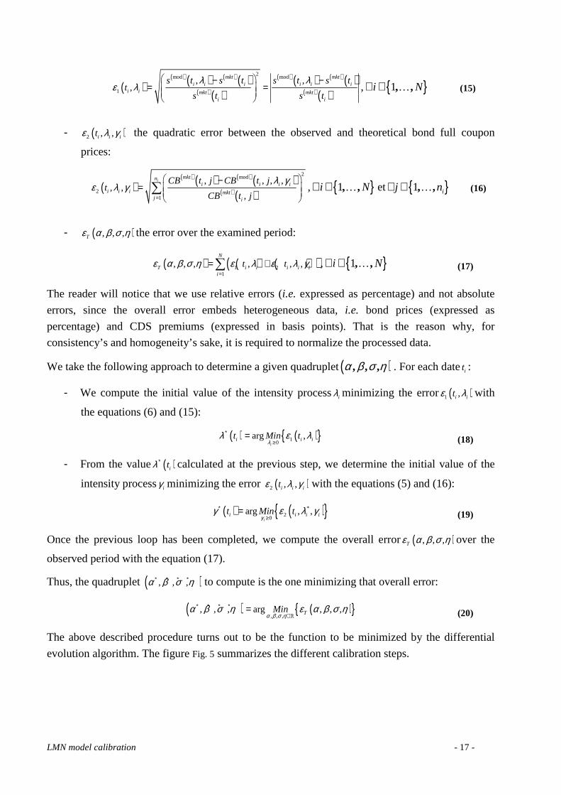
We take the following approach to determine a given quadruplet( ), , ,α β σ η . For each dateit :
- We compute the initial value of the intensity process iλ minimizing the error ( )1 ,i itε λ with
the equations (6) and (15):
( ) ( ){ }10
arg ,i
i i it Min tλ
λ ε λ∗
≥= (18)
- From the value ( )itλ∗ calculated at the previous step, we determine the initial value of the
intensity processiγ minimizing the error ( )2 , ,i i itε λ γ with the equations (5) and (16):
( ) ( ){ }*2
0arg , ,
ii i i it Min t
γγ ε λ γ∗
≥= (19)
Once the previous loop has been completed, we compute the overall error ( ), , ,Tε α β σ η over the
observed period with the equation (17).
Thus, the quadruplet ( ), , ,α β σ η∗ ∗ ∗ ∗ to compute is the one minimizing that overall error:
( ) ( ){ }, , ,
, , , arg , , ,TMinα β σ η
α β σ η ε α β σ η∗ ∗ ∗ ∗
∈=
ℝ (20)
The above described procedure turns out to be the function to be minimized by the differential
evolution algorithm. The figure Fig. 5 summarizes the different calibration steps.
LMN model calibration - 18 -
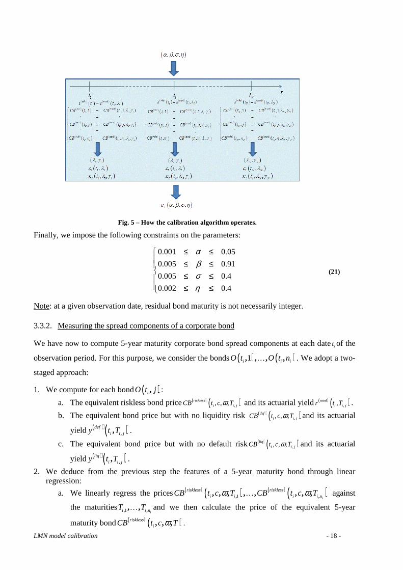
Fig. 5 – How the calibration algorithm operates.
Finally, we impose the following constraints on the parameters:
0.001 0.05
0.005 0.91
0.005 0.4
0.002 0.4
αβση
≤ ≤ ≤ ≤ ≤ ≤ ≤ ≤
(21)
Note: at a given observation date, residual bond maturity is not necessarily integer.
3.3.2. Measuring the spread components of a corporate bond
We have now to compute 5-year maturity corporate bond spread components at each dateit of the
observation period. For this purpose, we consider the bonds ( ) ( )1, , , ,i i iO t O t n… . We adopt a two-
staged approach:
1. We compute for each bond( ),iO t j :
a. The equivalent riskless bond price( ) ( ),, , ,risklessi i jCB t c Tω and its actuarial yield( ) ( )mod
,,i i jr t T .
b. The equivalent bond price but with no liquidity risk ( ) ( ),, , ,defi i jCB t c Tω and its actuarial
yield ( ) ( ),,defi i jy t T .
c. The equivalent bond price but with no default risk( ) ( ),, , ,liqi i jCB t c Tω and its actuarial
yield ( ) ( ),,liqi i jy t T .
2. We deduce from the previous step the features of a 5-year maturity bond through linear regression:
a. We linearly regress the prices ( ) ( ) ( ) ( )1, ,, , , , , , , ,i
riskless risklessi i i i nCB t c T CB t c Tω ω… against
the maturities 1, ,, ,ii i nT T… and we then calculate the price of the equivalent 5-year
maturity bond ( ) ( ), , ,risklessiCB t c Tω .

LMN model calibration - 19 -
b. Likewise, we linearly regress the yields( ) ( ) ( ) ( )1mod mod
, ,, , , ,ii i i i nr t T r t T… against the
maturities 1, ,, ,ii i nT T… and we then calculate the actuarial yield of the equivalent 5-year
maturity bond ( ) ( )mod ,ir t T .
c. We similarly operate with the prices ( ) ( ) ( ) ( )1, ,, , , , , , , ,i
def defi i i i nCB t c T CB t c Tω ω… which
we linearly regress against the maturities1, ,, ,ii i nT T… and we then calculate the price of
the equivalent 5-year maturity bond ( ) ( ), , ,defiCB t c Tω .
d. We linearly regress the yields( ) ( ) ( ) ( )1, ,, , , ,i
def defi i i i ny t T y t T… against the maturities
1, ,, ,ii i nT T… and we then calculate the actuarial yield of the equivalent 5-year maturity
bond ( ) ( ),liqiy t T .
e. We do the same with the prices ( ) ( ) ( ) ( )1, ,, , , , , , , ,i
liq liqi i i i nCB t c T CB t c Tω ω… which we
linearly regress against the maturities 1, ,, ,ii i nT T… and we then calculate the price of the
equivalent 5-year maturity bond ( ) ( ), , ,liqiCB t c Tω .
f. We linearly regress the yields( ) ( ) ( ) ( )1, ,, , , ,i
liq liqi i i i ny t T y t T… against the maturities
1, ,, ,ii i nT T… and we then calculate the actuarial yield of the equivalent 5-year maturity
bond ( ) ( ),liqiy t T .
The figures Fig. 6 and Fig. 7 describe how the bond price ( )P τ is computed between two coupon
payments.
Fig. 6 – Diagram of the flows of a bond with 0Nd d τ− − -year residual maturity.
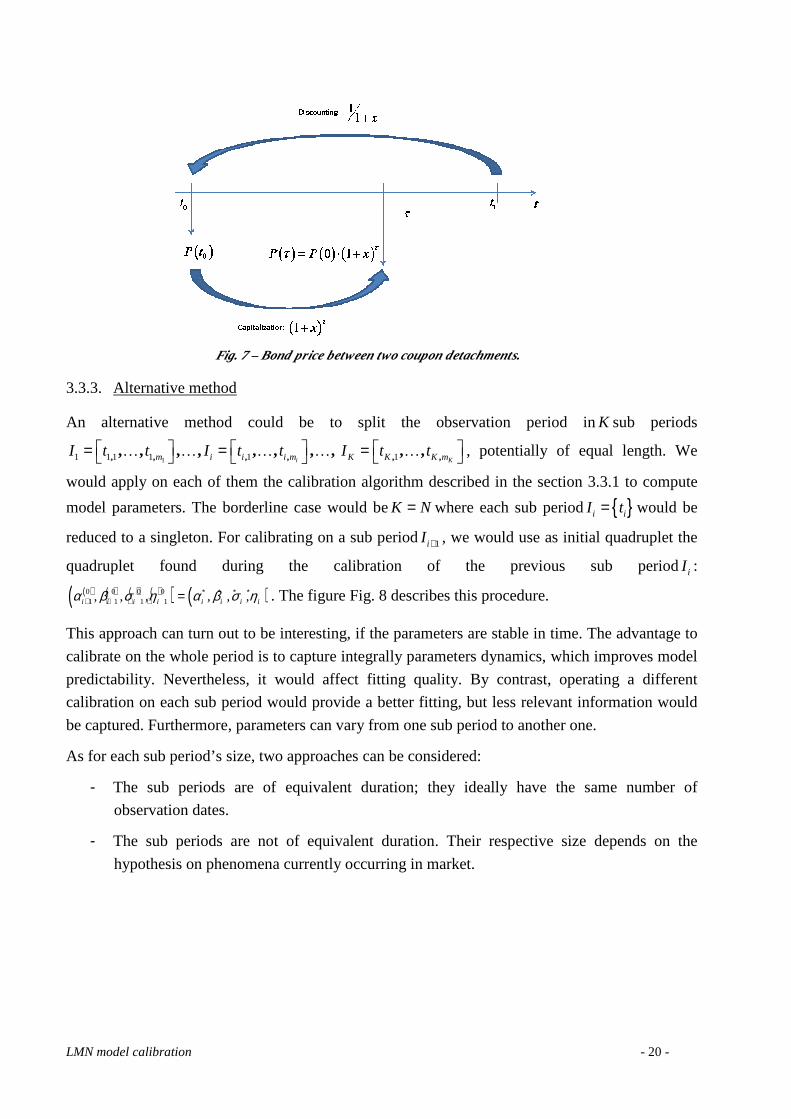
LMN model calibration - 20 -
Fig. 7 – Bond price between two coupon detachments.
3.3.3. Alternative method
An alternative method could be to split the observation period inK sub periods
11 1 1 1 1 1 , , , , , ,, , , , , , , , , ,i Km i i i m K K K mI t t I t t I t t = = = … … … … … , potentially of equal length. We
would apply on each of them the calibration algorithm described in the section 3.3.1 to compute
model parameters. The borderline case would beK N= where each sub period { }i iI t= would be
reduced to a singleton. For calibrating on a sub period 1iI + , we would use as initial quadruplet the
quadruplet found during the calibration of the previous sub periodiI :
( ) ( ) ( ) ( )( ) ( )0 0 0 01 1 1 1, , , , , ,i i i i i i i iα β σ η α β σ η∗ ∗ ∗ ∗
+ + + + = . The figure Fig. 8 describes this procedure.
This approach can turn out to be interesting, if the parameters are stable in time. The advantage to
calibrate on the whole period is to capture integrally parameters dynamics, which improves model
predictability. Nevertheless, it would affect fitting quality. By contrast, operating a different
calibration on each sub period would provide a better fitting, but less relevant information would
be captured. Furthermore, parameters can vary from one sub period to another one.
As for each sub period’s size, two approaches can be considered:
- The sub periods are of equivalent duration; they ideally have the same number of
observation dates.
- The sub periods are not of equivalent duration. Their respective size depends on the
hypothesis on phenomena currently occurring in market.

LMN model calibration - 21 -
Fig. 8 – Splitting of the observed period into several sub periods potentially of equivalent duration.
To conclude, we will not choose this method, because it is more suitable to focus on model
predictability for implementing an ESG.
4. ANALYSING THE RESULTS
In this section, we will comment the fitting quality obtained for the securities used in the
calibration process, we will analyse the different components of the spread of a corporate bond
and finally we will examined the results obtained from the out of sample test.
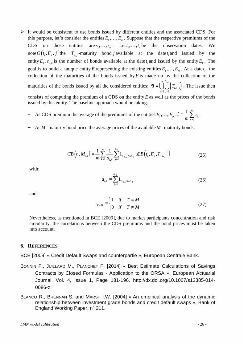
4.1. FITTING QUALITY
Fitting is nearly perfect for the CDS. As for the bonds, fitting is satisfactory, the error being less
than 6.20%, as the figure Fig. 12 in the appendix shows. The tableTab. 4 displays the parameter
values determined in this way.
α β σ η
0.006585229 0.005000000 0.007124079 0.040527902 Tab. 4 – Parameters optimal values.
As shown in the figure Fig. 9, the intensity process tends to be higher (with a 100% ratio at several
quotation dates) and “jerkier” than the liquidity process. Those observations will be corroborated
at the section 4.2. Other tables and graphs are available at the section 7.1 in the appendix.
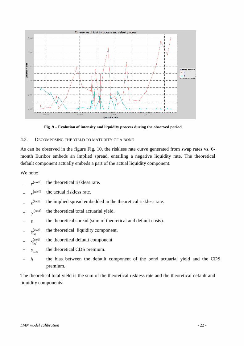
LMN model calibration - 22 -
Fig. 9 – Evolution of intensity and liquidity process during the observed period.
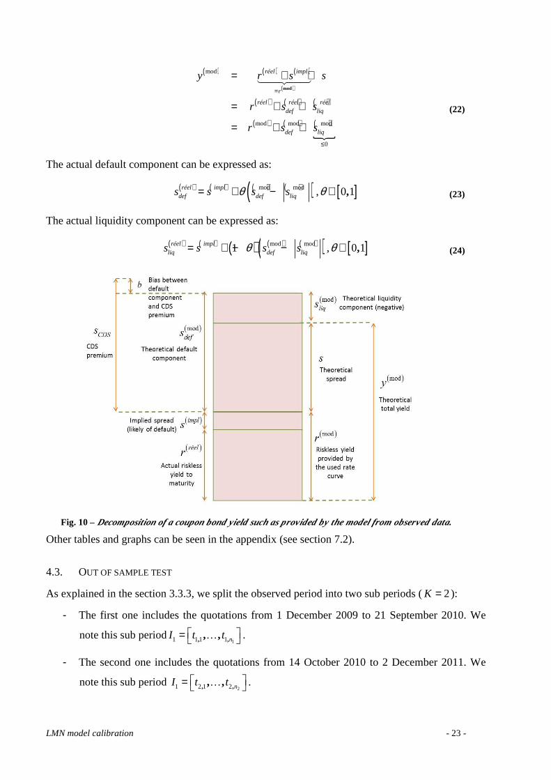
4.2. DECOMPOSING THE YIELD TO MATURITY OF A BOND
As can be observed in the figure Fig. 10, the riskless rate curve generated from swap rates vs. 6-
month Euribor embeds an implied spread, entailing a negative liquidity rate. The theoretical
default component actually embeds a part of the actual liquidity component.
We note:
− ( )modr the theoretical riskless rate.
− ( )réelr the actual riskless rate.
− ( )impls the implied spread embedded in the theoretical riskless rate.
− ( )mody the theoretical total actuarial yield.
− s the theoretical spread (sum of theoretical and default costs).
− ( )modliqs the theoretical liquidity component.
− ( )moddefs the theoretical default component.
− CDSs the theoretical CDS premium.
− b the bias between the default component of the bond actuarial yield and the CDS
premium.
The theoretical total yield is the sum of the theoretical riskless rate and the theoretical default and
liquidity components:
LMN model calibration - 23 -
( ) ( ) ( )
( )
( ) ( ) ( )
( ) ( ) ( )�
mod
mod mod mod
0
mod
réel impl
r
réel réel réeldef liq
def liq
y r s s
r s s
r s s
=
≤
= + +
= + +
= + +
�����
(22)
The actual default component can be expressed as:
( ) ( ) ( ) ( )( )mod modréel impldef def liqs s s sθ= + − , [ ]0 1,θ ∈ (23)
The actual liquidity component can be expressed as:
( ) ( ) ( ) ( ) ( )( )mod mod1réel implliq def liqs s s sθ= + − − , [ ]0 1,θ ∈ (24)
Fig. 10 – Decomposition of a coupon bond yield such as provided by the model from observed data.
Other tables and graphs can be seen in the appendix (see section 7.2).
4.3. OUT OF SAMPLE TEST
As explained in the section 3.3.3, we split the observed period into two sub periods ( 2K = ):
- The first one includes the quotations from 1 December 2009 to 21 September 2010. We
note this sub period11 1 1 1, ,, , nI t t = … .
- The second one includes the quotations from 14 October 2010 to 2 December 2011. We
note this sub period21 2 1 2 , ,, , nI t t = … .

LMN model calibration - 24 -
We calibrate the model from data included in the sub period11 1 1 1, ,, , nI t t = … and we price the
different instruments at the dates22 2 1 2 nI t t = , ,, ,… with the previously computed parameters
values( )1 1 1 1, , ,α β σ η∗ ∗ ∗ ∗ . We then get the following values:
− ( ) ( )2 2mod
, ,,i is t λ∗ for the CDS premiums at the different dates2,it ( 21,i m∈ ).
− ( ) ( )2 2 2mod
, , ,, , ,i i iCB t j λ γ∗ ∗ for the bond prices at the dates 2,it ( 21,i m∈ and 21 ,, ij n∈� � �� � ).
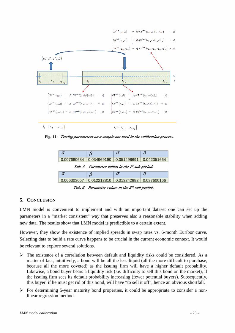
We then linearly regress the observed values( ) ( )2,mkt
is t and ( ) ( )2, ,mktiCB t j against the theoretical
values ( ) ( )2 2mod
, ,,i is t λ∗ and ( ) ( )2 2 2mod
, , ,, , ,i i iCB t j λ γ∗ ∗ for 21,i m∈ and 21 ,, ij n∈� � �� � . The figure Fig. 11
describes this procedure.
We finally operate several statistical tests:
− Newey-West test, − Test on Newey-West coefficients, − Jarque-Bera test, − Annova test.
We find that the test on Newey-West coefficients is conclusive for the CDS. Moreover,
predictability is satisfactory for the bonds DE000DB5S501 and DE000DB5S5U8. By contrast,
this is hardly the case for the bond DE000DB7URS2. Those results are anyway relevant given that
LMN algorithm is not predictable. The tables Tab. 5 and Tab. 6 present the parameter values
respectively in the 1st sub period and in the 2nd sub period. Parameters cannot be regarded as
stable. Fitting quality is obviously better than in the case of a calibration on the whole period. In
addition, for a given instrument, if the curves generated on the sub
periods11 1 1 1, ,, , nI t t = … and
22 2 1 2 nI t t = , ,, ,… are concatenated, the shape of such a curve looks
like the shape of the curve generated by calibrating on the whole period.
LMN model calibration - 25 -
Fig. 11 – Testing parameters on a sample not used in the calibration process.
α β σ η
0.007680684 0.034969190 0.051498691 0.042351664
Tab. 5 – Parameter values in the 1st sub period.
α β σ η
0.006303657 0.012212810 0.013242982 0.037600166
Tab. 6 – Parameter values in the 2nd sub period.
5. CONCLUSION
LMN model is convenient to implement and with an important dataset one can set up the
parameters in a “market consistent” way that preserves also a reasonable stability when adding
new data. The results show that LMN model is predictible to a certain extent.
However, they show the existence of implied spreads in swap rates vs. 6-month Euribor curve.
Selecting data to build a rate curve happens to be crucial in the current economic context. It would
be relevant to explore several solutions.
� The existence of a correlation between default and liquidity risks could be considered. As a matter of fact, intuitively, a bond will be all the less liquid (all the more difficult to purchase, because all the more coveted) as the issuing firm will have a higher default probability. Likewise, a bond buyer bears a liquidity risk (i.e. difficulty to sell this bond on the market), if the issuing firm sees its default probability increasing (fewer potential buyers). Subsequently, this buyer, if he must get rid of this bond, will have “to sell it off”, hence an obvious shortfall.
� For determining 5-year maturity bond properties, it could be appropriate to consider a non-linear regression method.
LMN model calibration - 26 -
� It would be consistent to use bonds issued by different entities and the associated CDS. For this purpose, let’s consider the entities1, , mE E… . Suppose that the respective premiums of the
CDS on those entities are1, , ms s… . Let 1, , nt t… be the observation dates. We
note ( ), ,i kO t E j the ,k jT -maturity bondj available at the dateit and issued by the
entity kE . ,i kn is the number of bonds available at the dateit and issued by the entitykE . The
goal is to build a unique entityE representing the existing entities1, , mE E… . At a dateit , the
collection of the maturities of the bonds issued byE is made up by the collection of the
maturities of the bonds issued by all the considered entities: { }1 1
,
, ,
i knm
i k jk j
T= =
=∪∪A . The issue then
consists of computing the premium of a CDS on the entity E as well as the prices of the bonds issued by this entity. The baseline approach would be taking:
− As CDS premium the average of the premiums of the entities 1, , mE E… :1
1ˆm
kk
s sm =
= ∑ .
− AsM -maturity bond price the average prices of the availableM -maturity bonds:
( ) ( )1 1
1 11
,
, , ,, , ,,
, , ,i k
i k j i l
nm
i i l T M i k i k jk ji k
CB t M CB t E Tm a =
= == ⋅∑ ∑ (25)
with:
1
1,
, , ,,
i k
i k j i l
n
i k T Mj
a ==
=∑ (26)
and:
1
10T M
if T M
if T M=
== ≠
(27)
Nevertheless, as mentioned in BCE [2009], due to market participants concentration and risk circularity, the correlations between the CDS premiums and the bond prices must be taken into account.
6. REFERENCES
BCE [2009] « Credit Default Swaps and counterpartie », European Centrale Bank.
BONNIN F., JUILLARD M., PLANCHET F. [2014] « Best Estimate Calculations of Savings Contracts by Closed Formulas - Application to the ORSA », European Actuarial Journal, Vol. 4, Issue 1, Page 181-196. http://dx.doi.org/10.1007/s13385-014-
0086-z.
BLANCO R., BRENNAN S. and MARSH I.W. [2004] « An empirical analysis of the dynamic relationship between investment grade bonds and credit default swaps », Bank of England Working Paper, no 211.

LMN model calibration - 27 -
DUFFIE D. [1998] « Defaultable term structure models with fractional recovery of par », Stanford University, Working paper.
DUFFIE D., JUN P. and KENNETH J. S. [1999] « Credit Swap Valuation », Financial Analysts Journal, no 55, 73‑ 87.
EIOPA [2014] Technical Specification for the Preparatory Phase (Part I), EIOPA-14/209
GILLI M., GROßE S. and SCHUMANN E. [2010] « Calibrating the Nelson–Siegel–Svensson model », COMISEF WORKING PAPERS SERIES, no 31.
LANDO D. [1998] « On Cox processes and credit risky securities », Review of Derivatives Research, vol. 2, no 2-3, 99‑ 120.
LONGSTAFF F.A., MITHAL S. and NEIS E. [2005] « Corporate Yield Spreads: Default Risk or Liquidity? New Evidence from the Credit Default Swap Market »,The Journal of Finance, vol. LX, no 5, 2213‑ 2253.
MOUDIKI T. [2014] « Sensibilité d’une rente viagère à l’extrapolation de la courbe de taux dans un contexte LTGA », Bulletin Français d'Actuariat, vol. 14, n°27.
NELSON C.R. and SIEGEL A.F. [1987] « Parsimonious Modeling of Yield Curves », Journal of Business, vol. 60, no 4, 473‑ 489.
OUAJJOU M.A. [2010] « Risque de crédit », Actuarial Thesis, ISUP.
PLANCHET F., THÉROND P.E., JUILLARD M. [2011] Modèles financiers en assurance. Analyses de risques dynamiques - seconde édition revue et augmentée, Paris : Economica (première édition : 2005).
STORN R. and PRICE K. [1997] « Differential Evolution – A Simple and Efficient Heuristic for Global Optimization over Continuous Spaces », Journal of Global Optimization, vol. 11, 341‑ 359.
SVENSSON L.E.O. [1994] « Estimating and Interpreting Forward Interest Rates: Sweden 1992–1994 », IMF Working Paper, 94‑ 114.
7. APPENDIX
In this appendix, the reader will find all the other graphics and tables relative to results obtained in
this paper.
LMN model calibration - 28 -
7.1. FITTING QUALITY
DE000DB5S5U8 DE000DB5S501 DE000DB7URS2 5-year maturity bond
CDS
Average -2,31% 2,92% 3,10% 1,05% 0,00% Standard
deviation 1,53%
1,34% 1,42% 1,13%
0,00%
Minimum 0,14% 0,26% 0,15% 0,02% 0,00% Maximum 6,20% 5,61% 5,01% 2,58% 0,00%
Tab. 7 – Fitting quality (error in % ) for the used instruments.
Fig. 12 – Fitting quality of coupon bonds.
LMN model calibration - 29 -
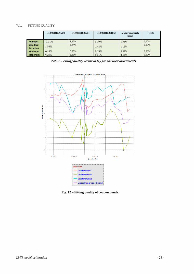
7.2. DECOMPOSING THE YIELD TO MATURITY OF A BOND
Fig. 13 – Time series of the different components of the 5-year maturity bond yield.
Fig. 14 – Bias is always negative during the observed period.
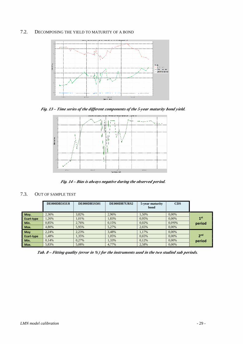
7.3. OUT OF SAMPLE TEST
DE000DB5S5U8 DE000DB5S501 DE000DB7URS2 5-year maturity bond
CDS
Moy. 2,36% 3,82% 2,96% 1,50% 0,00% 1st
period
Ecart-type 1,26% 1,01% 1,83% 0,95% 0,00% Min. 0,85% 2,76% 0,15% 0,02% 0,0²0% Max. 4,80% 5,95% 5,27% 2,65% 0,00%
Moy 2,24% 2,23% 3,48% 1,17% 0,00% 2nd
period
Ecart-type 1,48% 1,35% 1,05% 0,65% 0,00% Min. 0,14% 0,27% 1,33% 0,12% 0,00% Max. 5,83% 5,08% 4,77% 2,58% 0,00%
Tab. 8 – Fitting quality (error in % ) for the instruments used in the two studied sub periods.
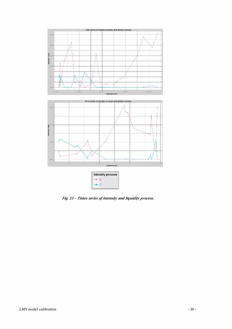
LMN model calibration - 30 -
Fig. 15 – Times series of intensity and liquidity process.