Derivative Free Trust Region Algorithms for Stochastic Optimizationanton/truststoch3.pdf ·...

Derivative Free Trust Region Algorithms for Stochastic

Optimization

Vijay Bharadwaj

Anton J. Kleywegt

School of Industrial and Systems Engineering

Georgia Institute of Technology

Atlanta, GA 30332-0205

September 7, 2008

1 Introduction and Review of Related Literature

In this article we study the following stochastic optimization problem. Let (Ω,F ,P) be a probability space.

Let ζ(ω) (where ω denotes a generic element of Ω) be a random variable on (Ω,F ,P), taking values in

the probability space (Ξ,G,Q), where Q denotes the probability measure of ζ. Suppose for some open set

E ⊂ Rl, F : E × Ξ �→ R is a real-valued function such that for each x ∈ E , F (x, ·) : Ξ �→ R is G-measurable

and integrable. Then, given a closed and convex set X ⊂ E , we consider the problem

minx∈X

{f(x) := EQ [F (x, ζ)]} (P)

If f is sufficiently smooth on X and its higher order derivatives can be computed exactly without much

effort at any x ∈ X , then there are many deterministic optimization techniques that can be used to solve

problem (P). However, in many practical problems, one is faced with the following conditions.

• For a given x ∈ X and ζ ∈ Ξ, F (x, ζ) can easily be computed exactly.

• It is prohibitively expensive to compute f(x) or its higher order derivatives exactly at any x ∈ X ,

typically because it is difficult to compute the (often multidimensional) integral that defines f(x).

• For a fixed x ∈ X and ζ ∈ Ξ, ∇xF (x, ζ) can not easily be computed exactly, or may not even exist at

all (x, ζ), even though f is differentiable at all x.

For example, one may have a simulator that takes x as input, generates ζ according to a specified

distribution, and computes F (x, ζ) with a single simulation run. Often such a simulator does not compute

1

∇xF (x, ζ). This may be because the simulator code required to compute ∇xF (x, ζ) is so complicated that

the analyst does not want to take the time and effort to do the coding or run the risk of introducing errors

in the code. It may also be that simulator is a black box to the user who wants to do the optimization

and the simulator only returns F (x, ζ) for a given x, and the user cannot or does not want to change the

simulator to also compute ∇xF (x, ζ). Also, as mentioned above, it may be that ∇xF (x, ζ) does not exist at

all (x, ζ) even though f is differentiable at all x. A combination of these reasons held in an application that

the authors worked on, and motivated the work in this paper.

Under the above assumptions it is natural to approximate f using a sample average function that can be

obtained at a relatively low cost as follows. In order to show how this is done, consider for some N ∈ N, a

sequence{ζj(ω)

}j∈N

of i.i.d. random functions on (Ω,F ,P) taking values in Ξ such that ζj is F-measurable

for each j ∈ N and P is such that Q is the measure induced on (Ξ,G) by ζ1. Then, we define the sample

average function fN : Rl × Ω −→ R as

fN (x, ω) :=1N

N∑j=1

F (x, ζj(ω)) (1)

Then for each x ∈ Rl, fN (x, ω) is an unbiased and consistent estimator of f(x). That is, EP[fN (x, ω)] = f(x)

and

limN→∞

fN (x, ω) = f(x) for P-almost all ω

The above result follows from the strong law of large numbers. Similarly, under some stronger conditions

on the probability spaces and the differentiability of the function F (·, ζ) with respect to x, it is possible to

show that the random function ∇fN : Rl × Ω −→ R

l defined as

∇fN (x, ω) :=1N

N∑j=1

∇xF (x, ζj(ω))

is an unbiased and consistent estimator of ∇f(x) for each x ∈ Rl. Given any x ∈ X and N ∈ N, in order

to evaluate the sample average function for some fixed ω ∈ Ω, we must be able to generate the independent

replications {ζj = ζj(ω) : j = 1, . . . , N}. In practice, ζ is usually a real-valued random vector and hence the

set {ζj : j = 1, . . . , N} can be obtained by first generating a set {ξ1, . . . , ξN} of pseudo-random numbers that

are independent and uniformly distributed on [0, 1] and subsequently applying an appropriate transformation

to this set.

There are two essentially different ways in which such sampling techniques can be incorporated in al-

gorithms that solve the problem (P). First, let us consider the class of algorithms popularly known as the

stochastic approximation approach. A description of the simplest algorithm in this class (first proposed in

?) is sufficient to illustrate the basic sampling strategy. The algorithm essentially generates a sequence of

{xn}n∈N⊂ X , starting at some x0 ∈ X , by applying the following recursion.

xn+1 = ΠX

(xn − αn∇f(xn)

)(2)

2

In (2), ΠX denotes the projection operation onto the set X and ∇f(xn) is an estimate of ∇f(xn) which

is obtained for each iteration n as follows. For some sample size N ∈ N, we first generate N independent

replications {ζjn : j = 1, . . . , N} of the random vector ζ, that are also independent of all replications generated

in earlier iterations. Then, we set

∇f(xn) :=1N

N∑j=1

∇xF (xn, ζjn)

Further, the sequence {αn}n∈Nof positive step-sizes is chosen to satisfy

∞∑n=1

αn = ∞ and∞∑

n=1

α2n < ∞

Under certain regularity conditions, it can be shown that the sequence {xn}n∈N(which is a sequence of

random vectors) converges with probability one, to a local minimum of f in X . Such an approach is

attractive because of its relative ease of implementation. However, in practice this approach has been found

to be extremely sensitive to the choice of the sequence {αn}n∈Nof step-sizes; a bad choice of which can lead

to an extremely slow rate of convergence. Therefore, subsequent work in this area has aimed to improve the

rate of convergence of this algorithm by averaging the gradient estimates obtained in consecutive iterations

along with the use of adaptive step-size sequences. Further, the algorithm has also been applied to non-

smooth problems where an estimate of a sub-gradient of the objective function is obtained through sampling

at each iteration. We refer the reader to ?, (?) and (?) for details. Also, ? and ? contain detailed treatments

of stochastic approximation algorithms for various cases.

The second approach, known variously as stochastic counterpart method, sample path optimization and

sample average approximation, works as follows. We first fix some ω ∈ Ω and some N ∈ N, and generate N

independent replications of the random vector ζ denoted by {ζj = ζj(ω) : j = 1, . . . , N}. Then, using this

fixed sample, we solve the optimization problem

minx∈X

fN (x, ω) :=1N

N∑j=1

F (x, ζj) (P)

Now, it is easily seen that fN (·, ω) is a deterministic function of x, we can compute fN (x, ω) and its higher

order derivatives (if they exist) exactly for any x ∈ X . Therefore, the problem (P) can be solved using any

appropriate deterministic optimization algorithm. This is certainly an appealing feature since there exist

a vast store of algorithms developed for deterministic optimization from which this choice can be made.

Suppose that

v∗N (ω) := min

x∈XfN (x, ω) and x∗

N (ω) ∈ arg minx∈X

fN (x, ω),

Then, it can be shown under mild conditions that as N →∞, v∗N and x∗

N converge respectively to the optimal

objective value and optimal solution of the “true” problem (P), for P-almost all ω. Further, there is a well-

developed theory of statistical inference for the optimal value v∗N and optimal solution x∗

N of the problem (P)

3

that helps in setting the sample size N and in the design of stopping tests. In particular, given any candidate

optimal solution x∗ ∈ X for the true problem, ? shows how the optimality gap f(x∗) − minx∈X f(x) can

be estimated by solving M sample average problems as in (P) for M independent realizations {ω1, . . . , ωM}.The same article also provides methods to statistically test the validity of the first order Karush-Kuhn-Tucker

optimality conditions for the point x∗ using an independently generated estimate of the gradient ∇f(x∗).

We refer the reader to ? and ? for details regarding the stochastic counterpart method and to ? and ? for

a general description of Monte Carlo sampling methods in the solution of stochastic programs.

In this paper, we deal with a specific class of stochastic programs that satisfy, apart from the previously

stated assumptions regarding the intractability of computing f or its higher order derivatives, the following

assumptions.

A 1. (a) The cost of computing F (x, ζ) for a given x ∈ Rl and ζ ∈ Ξ, while being small relative to the

cost of computing f(x), is still large enough to warrant attempts to lower the number of evaluations of

F (x, ζ) as much as possible.

(b) No sensitivity measures related to F can be computed directly. That is, if F (·, ζ) is continuously differ-

entiable with respect to x for some ζ ∈ Ξ, then we assume that ∇xF (x, ζ) cannot be evaluated for any

x ∈ X . Otherwise, if F (·, ζ) is convex for some ζ ∈ Ξ, then we assume that a subgradient cannot be

computed for any x ∈ X .

(c) The function f is continuously differentiable on E.

Indeed, the first two statements of Assumption A 1 hold quite often in the case of simulation optimization.

In many practical settings, F (x, ζ) is computed by a large and complex computer simulation model whose

source code is proprietary and hence unavailable. Obviously apart from making the computation of F (x, ζ)

very expensive , such a situation also precludes the use of automatic differentiation techniques to calculate

the gradient ∇xF (x, ζ) (if we know it exists).

If F (·, ζ) is continuously differentiable on E for Q-almost all ζ, then it is easy to see that f is also

continuously differentiable on E . However, many examples of stochastic optimization problems exist where

the f is continuously differentiable on E even when F (·, ζ) is only Lipschitz continuous on E for any ζ ∈ Ξ.

The following is a simple example of such a situation.

Example 1.1. Consider the well known news-vendor problem. A company has to decide the quantity x of

a seasonal product, to order. The product can be purchased at a unit cost of c and sold at a unit price of

r > c while in season. After that however, the remaining unsold stock can only be sold at a unit salvage

price of s, where s < c. Suppose further, that the demand ζ ∈ R+ for that product is uncertain and has

a distribution function G : R −→ [0, 1] associated with it that is continuous on R. In order to make the

4

decision regarding the quantity x, the company wishes to solve the optimization problem

maxx∈[0,∞)

f(x) := E[F (x, ζ)]

where the profit F : R+ × R+ −→ R can be written for any fixed x and ζ as

F (x, ζ) :=

⎧⎨⎩(s− c)x + (r − s)ζ if x ≥ ζ

(r − c)x if x < ζ

Indeed, for any given ζ ≥ 0, F (·, ζ) is not differentiable at x = ζ.

However, the expected value of the profit, f : R+ −→ R can be shown to be given for any x ∈ R+, by

f(x) = E [F (x, ζ)]

=∫

(−∞,∞)

F (x, ζ)dG(ζ)

= (r − c)x − (r − s)∫

[0,x]

G(ζ)dζ

Since G is known to be continuous on R, it follows that f is continuously differentiable on R+.

It can be shown that the same situation occurs in many two stage stochastic linear programming problems,

where the random data have densities associated with their distributions.

Assumption A 1 immediately suggests that any sampling-based solution methodology used on (P) should

attempt to incorporate the following features.

• The sample sizes used in the algorithm have to remain manageable small. Of course, more precise

statements regarding the sample size can be made only if the computational effort required to evaluate

F (x, ζ) and the total available computational budget are known.

• Once F (x, ζ) is evaluated for a given x and ζ, this value must be reused as much as possible.

Now, let us again consider the two approaches to solving the problem (P) that we discussed earlier, in light of

Assumption A 1 and the above requirements. In the case of stochastic approximation, the same algorithmic

recursion as in (2) can be used along with a biased gradient estimator which is generated as follows. Given

xn ∈ X , cn > 0 and some N ∈ N, we generate independent realizations ζijn ∈ Ξ for i = 0, . . . , l (where l is

the dimension of the search space) and j = 1, . . . , N , that are also independent of all realizations generated

earlier in the procedure. Then, we define the gradient estimator as

∇f(xn) :=

⎛⎜⎜⎜⎝

PNj=1 F (xn+cne1,ζ1j

n )−PNj=1 F (xn,ζ0j

n )

Ncn

...PN

j=1 F (xn+cnel,ζljn )−PN

j=1 F (xn,ζ0jn )

Ncn

⎞⎟⎟⎟⎠

5

where ei denotes the unit vector in the i-th coordinate direction in Rl. Essentially, this is a finite difference

gradient approximation where the function values f(xn + cnei) for i = 1, . . . , l are approximated by sample

averages found using independently generated samples. This idea, first suggested in ?, has the advantage that

convergence can be shown even for a sample size N = 1. However, it is explicitly required in the algorithm

that each new gradient estimate be generated using independent samples. Therefore, each iteration of the

algorithm requires (l + 1)×N new evaluations of the function F . Thus, given also the slow progress of this

algorithm due to small step-sizes, the stated algorithm may not be suitable for solving (P) under Assumption

A 1. However, subsequent research in this field has resulted in the development of gradient approximations

that can be generated using at most 2N evaluations of F . Algorithms that use such gradient approximations

are collectively known in literature as Simultaneous Perturbation Stochastic Approximation(SPSA). A com-

bination of these gradient approximations, used along with adaptive step sizes, may prove useful in solving

(P). We refer the reader to ? for the basic SPSA algorithm and its convergence analysis.

In this paper however, in order to be able to reuse evaluations of F , we will not consider algorithms that

require independent samples to be generated at each iteration. Accordingly, let us look at the sample average

approximation approach in light of Assumption A 1. As we noted earlier, having fixed the sample size N

and some ω ∈ Ω, (P) becomes a deterministic optimization problem. With Assumption A 1 however, it is

clear that sensitivity measures of the sample average function fN (·, ω) like derivatives or subgradients, are

also unavailable. Fortunately, there exist several different types of iterative algorithms for the optimization

of deterministic functions, without the use of derivative information. The literature in this area of research

is quite extensive but not all the different approaches are suited for solving the problem (P) under the

assumption that function evaluations are expensive. Hence, we will mention only a couple of ideas that are

related to the approach that we propose in this paper, and refer the reader to ? for an excellent review of

the state of the art in derivative free algorithms.

The simplest approach may be to use a direct search algorithm, i.e., an algorithm that proceeds using only

direct comparisons of objective function values at different points. Common examples of such algorithms

include the simplex reflection algorithm of ? and the Parallel Direct Search and Multi-directional Search

algorithms proposed respectively in ? and ?. Indeed, if fN (·, ω) is not continuously differentiable on X ,

then there is often no other alternative but to use such direct search algorithms to solve (P). On the other

hand, if fN (·, ω) is smooth, then such algorithms tend to progress slower than algorithms that exploit the

smoothness of fN .

When fN (·, ω) is smooth, then one strategy is to use traditional algorithms for deterministic smooth

optimization but with finite difference approximations of the gradient (and if possible, the Hessian). But

again, in general, it is unlikely that function evaluations can be reused in such an algorithm. Indeed, it is

extremely improbable that at some iteration n, given the current solution xn, the function fN has already

6

been evaluated at xn + cnei where ei is a unit vector in some coordinate direction. Thus, it is highly likely

that such a method will require (l+1)×N new function evaluations at each iteration, in order to approximate

just the gradient.

Recently however, there has been considerable interest in trust region algorithms for derivative free

unconstrained deterministic optimization of smooth functions under the assumption that function evaluations

are expensive. The idea is that instead of trying to approximate the unavailable higher order derivatives

of the objective function, we could construct a polynomial model that approximates the objective function

itself in a neighborhood of interest, using interpolation. Let us explore this approach in greater detail since

its core ideas are also applicable to the class of algorithms that we propose in this paper. Assume for the

moment that the feasible set X = Rl and that fN (·, ω) : R

l −→ R is sufficiently smooth. At iteration n,

given the current iterate xn, we construct an interpolation set Yn with the appropriate number of points.

That is, if we are interested in approximating fN with a linear model then there are l + 1 parameters to be

determined and hence the set Yn must contain l+1 points including xn. Similarly, if the model is quadratic,

then Yn must contain 1 + l + l(l + 1)/2 points including xn. Obviously, we try to include as many points

in the interpolation set as possible, at which the function fN has been evaluated already. Then, we find the

parameters in the model mn : Rl −→ R using the interpolation equations

mn(xi) = fN (xi) for i = 1, . . . , |Yn| (3)

Finally, the model mn is optimized in a trust-region Tn := {x ∈ Rl : ‖x− xn‖ ≤ Δn} which (hopefully)

yields a point with a lower objective function value. The points in the interpolation set Yn and the trust

region radius Δn are updated as the algorithm progresses.

This idea has its origins in an algorithm proposed in ?, where the author proposed the use of a quadratic

interpolation model. Much later, ? suggested an algorithm for constrained optimization where both the

objective function and the constraints were modeled using linear interpolation. However, there is some

crucial insight regarding such methods in ? that relates the interpolation set Yn to the quality of the model

mn as an approximation to the objective function within the trust region. Consider a model function that

is traditionally used in trust region algorithms.

mn(x) := fN (xn, ω) + ∇fN (xn, ω)T (x− xn) +12(x− xn)T Hn(x− xn) (4)

In (4), either Hn ∈ Sl×l (where S

l×l is the space of real symmetric l×l matrices) is either set to be∇2fN (xn, ω)

or obtained using a quasi-Newton update. In any case, if fN (·, ω) ∈ C2(Tn) and∥∥∇2fN (x, ω)

∥∥2≤ Kn for

all x ∈ Tn , we can derive the following bound on |fN (x, ω)−mn(x)| for x ∈ Tn using the Taylor series

7

expansion of fN (·, ω) at xn.

|fN (x, ω)−mn(x)| =∣∣∣∣fN (x, ω) − fN (xn, ω) − ∇fN (xn, ω)T (x− xn) − 1

2(x− xn)T Hn(x− xn)

∣∣∣∣=

∣∣∣∣12(x− xn)T∇2fN (xn + tn(x− xn)) (x− xn) − 12(x− xn)T Hn(x− xn)

∣∣∣∣ where tn ∈ [0, 1]

≤∣∣∣∣‖Hn‖2 + Kn

2

∣∣∣∣×Δ2n (5)

Such a bound relating the accuracy of the model function to the trust region radius is critical to the proper

performance of any trust region algorithm.

Now, instead of (4), suppose a quadratic model given by

mn(x) := fN (xn, ω) + βTn (x− xn) +

12(x− xn)T Λn(x− xn), (6)

that is obtained by solving the interpolation equations in (3) for the components of β ∈ Rl and Λn ∈ S

l×l,

is used in a trust region algorithm. In order for such an algorithm to be successful, the interpolation points

in Yn must be chosen such that the resulting model satisfies a bound similar to that in (5). It is well

known that for a finite difference gradient approximation, the error in the approximation decreases to zero

as the step-size used to calculate the gradient approximation reduces to zero. Analogously, the interpolation

points in Yn must be chosen to lie in a sufficiently small neighborhood of xn in order for βn and Hn to be

accurate estimates of ∇fN (xn, ω) and ∇2fN (xn, ω) respectively. Further,it can be shown that under certain

conditions, as the points in Yn get progressively closer to xn, βn converges to ∇fN (xn, ω) and Hn converges

to ∇2fN (xn, ω). However, in order to obtain a bound similar to that in (5), it turns out the points in Yn

also have to satisfy certain geometric conditions imposed on their positions relative to xn. In particular, the

interpolating points cannot lie on any quadratic surface in Rl. If they do, then it can be shown that the

equations in (3) have multiple solutions and that there exist solutions that give rise to models mn that are

bad approximations of the objective function within the trust region. In order to avoid such a situation, in

practice we usually require that the interpolation points should be sufficiently far away from any quadratic

surface in Rl. An interpolation set that satisfies such a condition is referred to as being well poised.

? defined the set Yn for each n ∈ N to consist of l + l(l + 1)/2 points chosen entirely from points

at which the objective function had been previously evaluated and assumed that at each n ∈ N, Yn would

automatically satisfy the geometric requirement mentioned above. ? however, ensured that the interpolation

set is updated in such a way that it continues to be well poised throughout. All subsequent algorithms that fit

in this framework have included in some form or the other, methods to keep the interpolation set well-poised.

? suggested a variant that used quadratic models and showed how Lagrange interpolation polynomials could

be used to add new points to the interpolation set to ensure its well-poisedness. The same paper also reported

some promising numerical results. Further, ? gave the first convergence proof for such algorithms and also

showed how Newton Fundamental Polynomials can be used to build quadratic models even when there are

8

not sufficiently many points in the interpolation set to exactly specify a fully quadratic model. ? provides a

good introduction to the use of Lagrange and Newton polynomials in order to maintain the well-poisedness

of the interpolation set. ? proposed an interesting variant of this idea, where instead of evaluating the

objective function at new points purely in order to keep the interpolation set well-poised, the model function

is minimized over a modified (albeit non-convex) trust region, which ensures that the minimizer, when added

to the interpolation set, will keep it well-poised. The authors show significant gains over the use of finite

difference gradients along with quasi-Newton updates for the Hessian. In a series of recent papers, ?,(?)

and (?) has revisited the idea of using Lagrange interpolation polynomials and has also investigated quasi-

Newton-like updating formulas for the Hessian matrix of the model found using interpolation, in an attempt

to reduce the routine linear algebra work in each iteration.

Indeed, the computational experience reported in the references given above seems to indicate that

if the sample average function is smooth enough, then solving the sample average problem (P) using such

interpolation models can result in substantial reductions in the number of required evaluations of the function

F . However, rather than working with a fixed sample size N , we believe that further reduction in the number

of evaluations of F can be achieved by gradually increasing the sample size in an adaptive manner as the

algorithm progresses. The following considerations motivate this belief.

Recall that we are looking to solve the problem (P) and we wish to do this by generating a sequence

{xn}n∈N⊂ X of points with successively lower objective function values. However, instead of f , we have

access only to a sequence of sample average functions{

fN

}N∈N

that converge to f as the sample size

N increases to infinity. Thus, by solving the sample average problem (P), we generate a sequence with

successively lower values of the sample average function fN and hope that this sequence also achieves

reduction in the objective function. Under this setting, the following rationale naturally emerges.

• In the initial stages of the algorithm, when large reductions are possible in the value of f , a crude

approximation of the objective function may be sufficient to generate points with lower values of f .

Accordingly, a sample average approximating function fN obtained using a small sample size N may

be sufficient to achieve improvement. Therefore, it makes sense to start the optimization process with

a small sample size.

• Further, we should not use a large number of function evaluations in generating minute reductions in

the value of the sample average function unless we are confident that this will also lead to improvements

in the value of f . Therefore, we use a sample size N only as long as the reductions obtained in value

of fN are significant compared to some measure of the error between fN and f .

With this survey of some of the issues involved in the solution of (P) and various algorithmic approaches,

next we turn to a class of algorithms that incorporates the aforementioned refinements.

9

2 A Class of Derivative Free Trust Region Algorithms

In this paper, we propose and analyze a class of iterative algorithms for solving the problem (P) under

Assumption A 1, when f is continuously differentiable on X . Our class of algorithms incorporates Monte

Carlo sampling techniques along with the use of polynomial model functions in a trust region framework.

When the objective function f : X −→ R and its gradient ∇f(x) can be evaluated easily, a typical trust

region algorithm used to find the stationary points of f in X , works as follows.

Algorithm 1. Let us set the constants used in the algorithm as

0 < η1 ≤ η2 < 1 0 < σ1 ≤ σ2 < 1 Δmax > 0

Also let the initial feasible point be x0 ∈ X and the initial trust region radius be 0 < Δ0 < Δmax. Then, for

any iteration n and current solution xn ∈ X , we generate the next point xn+1 in the following manner.

Step 1: Define a model function mn : X −→ R that approximates f within a trust region Tn := {xn + d : ‖d‖ ≤ Δn}

Step 2: Find xn + dn ∈ arg min {mn(x) : x ∈ X ∩ Tn}.

Step 3: Evaluate

ρn =f(xn)− f(xn + dn)

mn(xn)−mn(xn + dn)

If ρn ≥ η1, then set xn+1 = xn + dn; else set xn+1 = xn.

Step 4: Update the trust region radius as,

Δn+1 ∈

⎧⎪⎪⎪⎨⎪⎪⎪⎩

[Δn,Δmax] if ρn ≥ η2

[σ2Δn,Δn] if ρn ∈ [η1, η2)

[σ1Δn, σ2Δn] if ρn < η1

Thus, at any iteration n, given the current iterate xn ∈ X , we first define trust region Tn, which is a

ball of radius Δn, centered at xn and defined in the norm ‖·‖ on Rl. We will refer to Δn as the trust region

radius and ‖·‖ as the trust region norm. Next, we define a model function mn : X → R that approximates

the function f in X ∩ Tn. Since f(xn) and ∇f(xn) can be evaluated easily, mn is defined to be a quadratic

function of the form,

mn(x) = f(xn) +∇f(xn)T (x− xn) +12(x− xn)T Hn(x− xn) (7)

where Hn ∈ Sl×l. Further, if ∇2f(xn) is also available, then we set Hn = ∇2f(xn). Otherwise Hn may

be obtained for example, via a quasi-Newton update. After defining the model function and trust region,

we find an approximate minimizer xn + dn for mn within the trust region Tn, that satisfies a minimum

improvement condition (which we will later elaborate on). We evaluate the relative improvement ρn, which

10

is the actual decrease in the value of f at xn + dn as compared to xn, divided by the decrease predicted by

mn. If there is sufficient decrease in the function f then we update the solution for the next iteration as

xn+1 = xn + dn and otherwise we set xn+1 = xn. Finally, depending on the relative improvement, we either

reduce, leave unchanged, or increase the trust region radius Δn for the next iteration.

In order to solve the optimization problem (P) under Assumption A 1, using a trust region algorithm,

several modifications have to be made to Algorithm 1. First, since f(x) cannot be evaluated exactly for

any x ∈ Rl, we will instead have to use sample averages where ever required. The use of sampling in our

algorithms is akin to the sample average approximation approach. That is, we fix ω ∈ Ω and generate the

sequence{ζi := ζi(ω)

}i∈N⊂ Ξ before we begin the optimization process. All the sample averages required

by the algorithm, are taken with respect to this sample. Therefore, as far as our algorithms are concerned,

our sample average functions are deterministic functions whose parameters are x ∈ Rl and the sample size

N . Accordingly, it will be convenient for us to discard the dependence on ω ∈ Ω from the notation for the

sample average functions and denote the sample average function for any x ∈ Rl and a sample size N ∈ N

as f(x,N), where f : Rl × N −→ R is given by

f(x,N) :=1N

N∑j=1

F (x, ζj) (8)

Obviously, the model function defined in (7) cannot be used since neither f(xn) nor ∇f(xn) can be

evaluated exactly. Therefore, we propose the following alternative model function.

mn(x) := f(xn, N0n) + ∇nf(xn)T (x− xn) +

12(x− xn)T ∇2

nf(xn)(x− xn) (9)

In (9), since f cannot be evaluated exactly, we fix a sample size N0n and use the sample average f(xn, N0

n) to

approximate f(xn). Similarly, ∇nf(xn) ∈ Rl and ∇2

nf(xn) ∈ Sl×l are approximations to the gradient∇f(xn)

and Hessian∇2f(xn) respectively, obtained as follows. We evaluate the sample averages f(xn+yin, N i

n) at Mn

points {xn+y1n, . . . , xn+yMn

n } in a neighborhood of xn using sample sizes N in ∈ N. We will refer to the points

{xn + yin : i = 1, . . . ,Mn} as design points and refer to the corresponding vectors as {yi

n : i = 1, . . . ,Mn}as perturbations. Then, we assign non-negative weights {w1

n, . . . , wMnn } to each of the design points and find

∇nf(xn) and ∇2nf(xn) such that,

(∇nf(xn), ∇2nf(xn)) ∈ arg min

(β,Λ)∈Rl×Sl×l

Mn∑i=1

[wi

n

{f(xn + yi

n, N in)− f(xn, N i

n)− βT yin −

12yi

n

TΛyi

n

}2]

(10)

Thus, our model function mn for each n ∈ N,is a quadratic polynomial which best fits (in the least squares

sense) the sample average function values at the design points. We will refer to mn as defined in (9) as the

regression model function, since we essentially perform linear regression to obtain the model.

It is well known that the success of any trust region algorithm depends crucially on its ability to monitor

and adaptively improve the accuracy of the model function in approximating the objective function within

11

the trust region. When a Taylor series based model function as in (7) is used in Algorithm 1, Steps 3 and 4

serve this purpose. At iteration n, the relative improvement ρn evaluated in Step 3, serves as an indicator

for the quality of the model. Whenever ρn is small (ρn < η1), a reduction in the trust region radius in Step

4, improves the accuracy of the model within the trust region.

However, when a regression model function as in (9) is used, its accuracy in approximating f within the

trust region depends not only on the trust region radius, but also on the quality of f(xn, N0n), ∇nf(xn)

and ∇2nf(xn) as approximations f(xn), ∇f(xn) and ∇2f(xn) respectively. Therefore, apart from controlling

the trust region radius, we must appropriately choose N0n, the number of design points Mn, the location

of the design points {xn + yin : i = 1, . . . , Mn}, the corresponding sample sizes {N i

n : i = 1, . . . ,Mn} and

weights {win : i = 1, . . . , Mn} for each n ∈ N so that the resulting model function may be sufficiently

accurate. Perhaps more importantly, in light of Assumption A 1, we must also seek to minimize the number

of evaluations of the function F used in the optimization process.

Accordingly, in Section 3, we consider the accuracy of the regression model function mn defined in (9) as

an approximation of f and describe procedures to pick the design points, sample sizes and weights required

to construct mn with a specified accuracy. Subsequently, we describe the working of a typical trust region

algorithm that uses such regression model functions and show its convergence in Section ??.

3 The Regression Model Function

In this section, we analyze the properties of the regression model function as defined in (9) and develop prac-

tical schemes to appropriately pick the design points, sample sizes and weights required for its construction.

Consider a sequence {xn}n∈N⊂ X where X ⊂ R

l is assumed to be closed. For each n ∈ N, we

suppose that f(xn, N0n) is calculated for some sample size N0

n. Also, we assume that the sample averages

{f(xn + yin, N i

n) : i = 1, . . . ,Mn} are evaluated at a set of design points {xn + yin : i = 1, . . . , Mn} ⊂ R

l

using the sample sizes {N in : i = 1, . . . ,Mn}. Finally, we assume that using a set of non-negative weights

{win : i = 1, . . . , Mn}, ∇nf(xn) ∈ R

l and ∇2nf(xn) ∈ S

l×l are determined to satisfy

(∇nf(xn), ∇2nf(xn)) ∈ arg min

(β,Λ)∈Rl×Sl×l

Mn∑i=1

[wi

n

{f(xn + yi


n)− βT yin −

12yi

n

TΛyi

n

}2]

(11)

Note: Actually, without loss of generality we can assume that win > 0 for i = 1, . . . ,Mn. This is because

setting win = 0 for some i ∈ {1, . . . , Mn} is equivalent to not including the design point xn + yi

n in the

set used to determine ∇nf(xn) and ∇2nf(xn). Therefore, we assume that only the points that had positive

weights associated with them, were included in the set of design points to begin with. For the same reason,

we also assume without loss of generality that∥∥yi

n

∥∥2

> 0 for each i = 1, . . . ,Mn and n ∈ N.

12

Our aim is to first establish when the accuracy of the regression model function approaches that of the

“exact” model function defined in (7) as n → ∞. In particular, we investigate the conditions that can be

placed on the choice of the various quantities required to find f(xn, N0n), ∇nf(xn) and ∇2

nf(xn), that are

sufficient to ensure∣∣∣f(xn, N0

n)− f(xn)∣∣∣ → 0,

∥∥∥∇nf(xn)−∇f(xn)∥∥∥

2→ 0 and

∥∥∥∇2nf(xn)−∇2f(xn)

∥∥∥2→ 0

as n→∞. Let us start with a result regarding∣∣∣f(xn, N0

n)− f(xn)∣∣∣.

Lemma 3.1. Suppose the following assumptions hold.

A 2. For any compact set D ⊂ E, f is continuous on D and the sequence{

f(·, N)}

N∈N

converges uniformly

to f on D.

limN→∞

supx∈D

∣∣∣f(x,N)− f(x)∣∣∣ = 0 (12)

A 3. The sequence{N0

n

}n∈N

of sample sizes satisfies N0n →∞ as n→∞.

Then, for any sequence {xn}n∈N⊂ C ⊂ X such that C is compact, we get

limn→∞

∣∣∣f(xn, N0n)− f(xn)

∣∣∣ = 0

In particular, if xn → x, then

limn→∞ f(xn, N0

n) = f(x)

Proof. We have for each n ∈ N.∣∣∣f(xn, N0n)− f(xn)

∣∣∣ ≤ supx∈C

∣∣∣f(x,N0n)− f(x)

∣∣∣Therefore, taking limits as n→∞ and noting that N0

n →∞, we get

limn→∞


∣∣∣ ≤ limn→∞ sup

x∈X

∣∣∣f(x,N0n)− f(x)

∣∣∣ = 0

Next, from the continuity of f on X , we get

limn→∞

∣∣∣f(xn, N0n)− f(x)

∣∣∣ ≤ limn→∞


∣∣∣+ limn→∞ |f(xn)− f(x)| = 0

Thus, we see that if we have uniform convergence of the sequence{

f(·, N)}

N∈N

of sample average

functions to the function f on some compact set C ⊃ {xn}n∈N, then the accuracy of f(xn, N0

n) as an

approximation to f(xn), can be improved by increasing the sample size N0n.

Next,we consider the accuracy of ∇nf(xn) and ∇2nf(xn) as approximations of ∇f(xn) and ∇2

nf(xn). In

particular, we will first consider conditions sufficient to ensure that

limn→∞

∥∥∥∇nf(xn)−∇f(xn)∥∥∥

2= 0

13

Accordingly, let us define the notation required to represent and characterize the set of optimal solutions on

the right side of (11). First, let the perturbation matrix Yn ∈ RMn×l be defined as

Yn :=

⎛⎜⎜⎜⎜⎜⎜⎝

(y1n)T

(y2n)T

...

(yMnn )T

⎞⎟⎟⎟⎟⎟⎟⎠ (13)

Let Nn := {N1n, . . . , NMn

n } denote the set of sample sizes used to evaluate the sample averages at the design

points. Define f(x, Yn,Nn) ∈ RMn for any x ∈ R

l as

f(xn, Yn,Nn) :=

⎛⎜⎜⎜⎜⎜⎜⎝

f(x + y2n, N2

n)− f(x,N2n)

f(x + y1n, N1

n)− f(x,N1n)

...

f(x + yMnn , NMn

n )− f(x,NMnn )

⎞⎟⎟⎟⎟⎟⎟⎠ (14)

Also, we define f(xn, Yn) ∈ RMn for any x ∈ R

l as

f(xn, Yn) :=

⎛⎜⎜⎜⎜⎜⎜⎝

f(x + y1n)− f(x)

f(x + y2n)− f(x)...

f(x + yMnn )− f(x)

⎞⎟⎟⎟⎟⎟⎟⎠ (15)

Next, we develop notation to represent the quadratic form yin

T Λyin in (11). Let y ∈ R

l be any vector and

H ∈ Sl×l be any symmetric matrix given by

y =

⎛⎜⎜⎜⎜⎜⎜⎝

y1

y2

...

yl

⎞⎟⎟⎟⎟⎟⎟⎠ and H =

⎛⎜⎜⎜⎜⎜⎜⎝

h11 h12 · · · h1l

h21 h22 · · · h2l

......

. . ....

hl1 hl2 · · · hll

⎞⎟⎟⎟⎟⎟⎟⎠

Then, the quadratic form yT Hy expands as follows.

yT Hy =l∑

j=1

l∑k=1

hjkyjyk

Since H is assumed to be symmetric we know that hjk = hkj for all j, k ∈ {1, . . . , l}. Thus,

yT Hy = 2l∑

j=1

l∑k=j+1

hjkyjyk +l∑

j=1

hjjy2j

Therefore,12yT Hy =

l∑j=1

l∑k=j+1

hjkyjyk +12

l∑j=1

hjjy2j

14

We wish to write the right side of the above equation as the scalar product of two appropriately defined

vectors. Accordingly, we define the vector yQ ∈ Rl(l+1)/2 corresponding to y ∈ R

l as

yQ :=(

y1y2, y1y3, y2y3, . . . , y1yl, y2yl, . . . , yl−1yl,1√2y21 , . . . ,

1√2y2

l

)T

(16)

=

({yjyk}j,k=1,...,l

j<k

, { 1√2y2

j }j=1,...,l

)T

Note the following useful relationship between the Euclidean norms of y and yQ:

∥∥yQ∥∥2

2=

12

⎡⎣ l∑

j=1

l∑k=j+1

2y2j y2

k +l∑

j=1

y4j

⎤⎦

=12

⎛⎝ l∑

j=1

y2j

⎞⎠2

=12‖y‖42 (17)

Similarly, we write the components of H as a vector Hv ∈ Rl(l+1)/2 as follows.

Hv :=(

h12, h13, h23, . . . , h1l, h2l, . . . , h(l−1)l,1√2h11,

1√2h22, . . . ,

1√2hll

)T

(18)

=

({hjk}j,k=1,...,l,

j<k

, { 1√2hjj}j=1,...,l

)T

Then it is not hard to see that,12yT Hy = HT

v yQ (19)

Using the notation in (16), let for each i ∈ {1, . . . , Mn},

yin

Q:=

((yi

n)1(yin)2, (yi

n)1(yin)3, (yi

n)2(yin)3, . . . , (yi

n)1(yin)l, (yi

n)2(yin)l, . . . , (yi

n)l−1(yin)l,

1√2(yi

n)21, . . . ,1√2(yi

n)2l

)T

where (yin)j denotes the jth component of yi

n. Also, define the matrix Y Qn ∈ R

Mn×l(l+1)/2 as

Y Qn :=

⎛⎜⎜⎜⎜⎜⎜⎜⎝

(y1

nQ)T

(y2

nQ)T

...(yMn

nQ)T

⎞⎟⎟⎟⎟⎟⎟⎟⎠

(20)

Let for each i = 1, . . . ,Mn, let zin

T :=(yi

nT (yi

nQ)T

). Define the regression matrix Zn ∈ R

Mn×(l+l(l+1)/2)

as

Zn :=

⎛⎜⎜⎜⎝

z1n

T

...

zMnn

T

⎞⎟⎟⎟⎠ (21)

15

Obviously, we have Zn =(Yn Y Q

n

). Finally, we let Wn = diag(w1

n, . . . , wMnn ). Now, we can write the set

of optimal solutions on the right side of (11) as follows.

arg min(β Λ)∈Rl×Sl×l

Mn∑i=1

[wi

n

{f(xn + yi


n)− βT yin −

12yi

n

TΛyi

n

}2]≡

arg min(β Λv)T ∈Rl+l(l+1)/2

∥∥∥∥∥∥√

Wn

⎧⎨⎩f(xn, Yn,Nn)− Zn

⎛⎝ β

Λv

⎞⎠⎫⎬⎭∥∥∥∥∥∥

2

2

(22)

Consider the optimization problem occurring on the right side of (22).

min(β Λv)T ∈Rl+l(l+1)/2

∥∥∥∥∥∥√

Wn


⎛⎝ β

Λv

⎞⎠⎫⎬⎭∥∥∥∥∥∥

2

2

(23)

It is easy to see that this optimization problem is equivalent to computing the weighted projection of the

vector f(xn, Yn,Nn) ∈ RMn on to the subspace of R

Mn spanned by the columns of Zn. We know that

such a projection always exists since a subspace is a closed convex set. Hence the set of optimal solutions

of the optimization problem in (23) has to be non-empty. Thus, (22) shows that our method of finding

∇nf(xn) ∈ Rl and ∇2

nf(xn) ∈ Sl×l such that (11) holds, is well defined. Also, it is easily seen that for the

existence of a unique optimal solution, the columns of Zn have to be linearly independent. Since there are

l components of ∇nf(xn) and l(l + 1)/2 components of ∇2nf(xn), Zn contains p := l + l(l + 1)/2 columns.

Thus, a unique optimal solution exists for (23) only if Zn contains at least p linearly independent rows.

It is well known that the projection problem in (23) can be solved by solving the so-called normal

equations associated with this problem. That is, we have

arg min(β Λv)T ∈Rp

∥∥∥∥∥∥√

Wn


⎛⎝ β

Λv

⎞⎠⎫⎬⎭∥∥∥∥∥∥

2

2

=

⎧⎨⎩⎛⎝ β

Λv

⎞⎠ ∈ R

p : (ZTn WnZn)

⎛⎝ β

Λv

⎞⎠ = ZT

n Wnf(xn, Yn,Nn)

⎫⎬⎭

Using the notation in (18), we define[∇2fn(x)

]v∈ R

l(l+1)/2 corresponding to ∇2fn(x) by

[∇2fn(x)

]v

=

({(∇2fn(x))jk

}j,k=1,...,l, j<k

,

{1√2(∇2fn(x))jj

}j=1,...,l

)T

(24)

where (∇2fn(x))jk denotes the element in the jth row and kth column of ∇2fn(x). Now, we finally get that

choosing ∇nf(xn) ∈ Rl and ∇2

nf(xn) ∈ Sl×l from (11) is equivalent to choosing the components of ∇nf(xn)

and[∇2

nf(xn)]

vfrom a solution of the set of linear equations given by,

(ZTn WnZn)

⎛⎝ ∇nf(xn)[∇2

nf(xn)]

v

⎞⎠ = ZT

n Wnf(xn, Yn,Nn) (25)

16

With this notation, we are ready to state conditions on the design points, sample sizes and weights

sufficient to ensure that∥∥∥∇nf(xn)−∇f(xn)

∥∥∥2→ 0 and

∥∥∥∇2nf(xn)−∇2f(xn)

∥∥∥2→ 0 as n → ∞, Let us

begin by considering some intuitive ideas that motivate our conditions.

Consider for a moment, the finite difference approximation ∇hg(x∗) ∈ Rl of the gradient ∇g(x∗) of some

function g ∈ C1(Rl) at some x∗ ∈ Rl, defined as

∇hg(x∗) :=

⎛⎜⎜⎜⎝

g(x∗+he1)−g(x∗)h

...g(x∗+hel)−g(x∗)

h

⎞⎟⎟⎟⎠

where {e1, . . . , el} represent unit vectors along the coordinate directions and h > 0 is the step size. It is easy

to see that such a gradient approximation is nothing but the gradient of the linear function

m(x) = g(x∗) + ∇hg(x∗)T (x− x∗)

that satisfies

∇hg(x∗) ∈ arg minβ∈Rl

{l∑

i=1

[g(x∗ + hei)− g(x∗)− hβT ei

]2}

Thus, a linear function m(x) with the finite difference gradient approximation ∇hg(xn), is the linear function

that best fits the function values {g(x + hei) : i = 1, . . . , l} at the corresponding design points {x + hei : i =

1, . . . , l}. Further, it is well known that

limh→0

∥∥∥∇hg(x∗)−∇g(x∗)∥∥∥

2= 0

That is , the finite difference approximation get progressively more accurate as the step size h, i.e., the

Euclidean distance between x∗ and the design points decreases to zero.

It is intuitive to expect that in the same fashion, the accuracies of ∇nf(xn) and ∇2nf(xn) determined

as in (11) depend on the Euclidean distances {∥∥yi

n

∥∥2

: i = 1, . . . , Mn} of the design points {xn + yin : i =

1, . . . ,Mn} from xn. Indeed, we should expect that in order to ensure∥∥∥∇nf(xn)−∇f(xn)

∥∥∥2→ 0 and∥∥∥∇2

nf(xn)−∇2f(xn)∥∥∥

2→ 0 as n → ∞, the Euclidean distances between the design points and the point

xn must decrease to zero as n → ∞. Thus, in order to monitor and control the Euclidean distances of the

design points from xn, we define a neighborhood of xn called the design region for each n, as follows.

Dn :={x ∈ R

l : ‖x− xn‖2 ≤ δn

}(26)

We will refer to δn > 0 as the design region radius for iteration n. Without loss of generality, we will assume

that∥∥yi

n

∥∥2≤ δn for i = 1, . . . ,M I

n for some M In ≤Mn and

∥∥yin

∥∥2

> δn for i = M In + 1, . . . , Mn. We use the

terms inner and outer to denote the design points lying respectively within and outside the design region.

In order to obtain the convergence of ∇nf(xn) to ∇f(xn) and ∇2nf(xn) to ∇2f(xn), we will ensure that

17

δn → 0 as n → ∞ while at the same time requiring a certain number of inner design points exist for each

n ∈ N.

For the notation that we defined earlier with regard the the design points, we will use the superscripts

“I” and “O” to denote the corresponding notation for the inner and outer design points respectively. Thus,

we let

Y In :=

⎛⎜⎜⎜⎝

y1n

T

...

yMI

nn

T

⎞⎟⎟⎟⎠ and Y O

n :=

⎛⎜⎜⎜⎝

yMI

n+1n

T

...

yMnn

T

⎞⎟⎟⎟⎠ and hence Yn =

⎛⎝Y I

n

Y ON

⎞⎠ (27)

and define the matrices Y In

Q, Y On

Q, ZIn and ZO

n in the same manner. Analogous to Nn, we let N In :=

{N1n, . . . , N

MIn

n } and NOn := {NMI

n+1n , . . . , NMn

n } denote the set of sample sizes used to evaluate the sample

average functions at the inner and outer design points respectively. Then, the vectors f(x, Y In ,N I

n) ⊂ RMI

n

and f(x, Y On ,NO

n ) ⊂ RMn−MI

n are defined analogous to f(x, Yn,Nn). Also, we let W In = diag

(w1

n, . . . , wMI

nn

)and WO

n = diag(w

MIn+1

n , . . . , wMnn

).

We noted earlier that as n→∞ we will ensure that δn → 0 as n→∞. This implies that

limn→∞ max

i=1,...,MIn

∥∥yin

∥∥2

= 0

That is, the inner perturbation vectors corresponding to larger n will be much smaller in norm that those

used earlier in the sequence. Therefore, in order to compare various sets of the design points for different

n ∈ N, we will scale the corresponding perturbations such that the corresponding design region radii are all

equal to 1. Accordingly, we define for each i = 1, . . . ,Mn and n ∈ N, the scaled perturbation vector yin ∈ R

l

and the scaled regression vector zin ∈ R

p

yin :=

yin

δnand zi

n :=

⎛⎝ yi

n

δn

(yin)Q

δ2n

⎞⎠ (28)

The corresponding scaled perturbation and regression matrices are defined as follows.

Yn :=

⎛⎜⎜⎜⎝

(y1n)T

...

(yMnn )T

⎞⎟⎟⎟⎠ =

Yn

δn(29)

Y Qn :=

⎛⎜⎜⎜⎜⎝{(y1

n)Q}T

δ2n

...{(yMn

n )}Q

δ2n

⎞⎟⎟⎟⎟⎠ =

Y Qn

δ2n

(30)

Zn :=(Yn Y Q

n

)= ZnDn (31)

18

where

Dn = diag

⎛⎜⎜⎜⎜⎝

1δn

, . . . ,1δn︸︷︷︸

l terms

,1δ2n

, . . . ,1δ2n︸︷︷︸

l(l+1)/2 terms

⎞⎟⎟⎟⎟⎠ (32)

The corresponding scaled matrices Y In , Y O

n , (Y In )Q, (Y O

n )Q, ZIn and ZO

n are defined analogously.

Also, note that we use sample averages of the form f(xn + yin, N i

n) for i = 1, . . . , Mn in the calcu-

lation of ∇nf(xn) and ∇2nf(xn) for each n ∈ N. In order to obtain

∥∥∥∇nf(xn)−∇f(xn)∥∥∥

2→ 0 and∥∥∥∇2

nf(xn)−∇2f(xn)∥∥∥

2→ 0 as n → ∞, since ∇f(xn) and ∇2f(xn) are quantities related to the function

f , it is intuitive to expect that the sequence{

f(·, N)}

N∈N

must converge to the the function f on X , in

a certain sense as the sample size N grows to ∞. For example, we already know from the strong law of

large numbers that the sequence∣∣∣f(x,N)− f(x)

∣∣∣→ 0 point wise for each x ∈ Rl such that f(x) is finite for

P-almost all ω. However, we require stronger forms of convergence of the sample average function f(·, N)

to f . With regard to such a requirement, let us define notation for the required function spaces and their

norms. First, for any D ⊂ Rl, let W0(D) denote the space of all Lipschitz continuous functions φ : D −→ R.

The standard norm (referred to as the Lipschitz norm) defined on W0(D) is as follows. For any φ ∈W0(D),

‖φ‖W0(D) := sup

x∈D|φ(x)| + sup

x,x+y∈Dy �=0

|φ(x)− φ(y)|‖y‖2

< ∞

As usual, we let C1(D) denote the space of continuously differentiable functions on D with

‖φ‖C1(D) = sup

x∈D|φ(x)| + sup

x∈D‖∇φ(x)‖2

Further, let W1(D) denote the space of Lipschitz continuously differentiable functions on D. That is φ ∈W1(D) if

‖φ‖W1(D) := sup

x∈D|φ(x)| + sup

x∈D‖∇φ(x)‖2 + sup

x,x+y∈Dy �=0

‖∇φ(x + y)−∇φ(x)‖2‖y‖2

< ∞

Finally, we let C2(D) denote the set of twice continuously differentiable functions on D. From the aforemen-

tioned definitions, it is clear that

W0(D) ⊃ C1(D) ⊃ W1(D) ⊃ C2(D)

Finally, using the notation we have developed so far, we note that,

ZTn WnZn =

⎛⎝ Y T

n WnYn Y Tn WnY Q

n

Y Qn

TWnYn Y Q

nTWnYn

⎞⎠ and ZT

n Wnf(xn, Yn,Nn) =

⎛⎝ Y T

n Wnf(xn, Yn,Nn)

Y Qn

TWnf(xn, Yn,Nn)

⎞⎠

Therefore, the system of equations in (25) can be divided into two sets of equations given below.

(Y Tn WnYn)∇fn(xn) + (Y T

n WnY Qn )

[∇2fn(xn)

]v

= Y Tn Wnf(xn, Yn,Nn) (33)(

Y Qn

TWnYn

)∇fn(xn) +

(Y Q

n

TWnY Q

n

) [∇2fn(xn)

]v

= Y Qn

TWnf(xn, Yn,Nn) (34)

19

While considering sufficient conditions to ensure that∥∥∥∇nf(xn)−∇f(xn)

∥∥∥2→ 0 as n → ∞, we will

assume that ∇nf(xn) and ∇2nf(xn) are picked satisfy only the first of the two sets of equations, i.e., the set

given in (33). Obviously, this is a weaker requirement that picking ∇nf(xn) and ∇2nf(xn) such that both

(33) and (34) are satisfied. Therefore the following result holds when ∇nf(xn) and ∇2nf(xn) are picked such

that (25) holds.

Theorem 3.2. Consider a sequence {xn}n∈N⊂ X and let for each n ∈ N, ∇nf(xn) ∈ R


l×l

be picked so as to satisfy (33). Suppose that the following assumptions hold.

A 4. For any compact set D ⊂ E, we have that f ∈ C1(D),{

f(·, N)}

N∈N

⊂W0(D) and

limN→∞

∥∥∥f(·, N)− f∥∥∥

W0(D)= 0

A 5. The sample sizes N in corresponding to the inner design points all increase to infinity as n→∞. That

is,

limn→∞ min

i=1,...,MIn

N in = ∞

A 6. The sequence {δn}n∈Nof design region radii is such that δn > 0 for each n ∈ N and δn → 0 as n→∞.

A 7. The set of design points{xn + yi

n : i = 1, . . . ,Mn and n ∈ N}

and the sequence {Wn}n∈Nof weight

matrices, satisfy the following.

1. There exists a compact set C ⊂ E such that the point xn and the set of design points {xn + yin : i =

1, . . . , Mn} satisfy

xn ∈ C and {xn + yin : i = 1, . . . ,Mn} ⊂ C (35)

for each n ∈ N.

2. There exists KIλ <∞ such that for each n ∈ N,∥∥∥(Y I

n )T W In Y I

n

∥∥∥2

∥∥∥((Y In )T W I

n Y In )−1

∥∥∥2

< KIλ (36)

3.

limn→∞

∥∥∥(Y On )T WO

n Y On

∥∥∥2∥∥∥(Y I

n )T W In Y I

n

∥∥∥2

= 0 (37)

A 8. The sequence of Hessian approximation matrices{∇2fn(xn)

}n∈N

is norm-bounded. That is, there

exists KH <∞ such that∥∥∥∇2fn(xn)

∥∥∥2

< KH for all n ∈ N.

Then, it holds that

limn→∞

∥∥∥∇nf(xn)−∇f(xn)∥∥∥

2= 0

In particular, if {xn}n∈N⊂ X is such that xn → x ∈ X as n→∞, then

limn→∞ ∇nf(xn) = ∇f(x)

20

We will first show a couple of useful Lemmas and then proceed with the proof of Theorem 3.2. For

the next lemma, and for the rest of this article, we will let λmax(A) and λmin(A) denote respectively the

maximum and minimum eigenvalues of any square matrix A.

Lemma 3.3. Let Assumption A 7 hold. Then, Y Tn WnYn is positive definite for each n ∈ N and the following

assertions hold.

1. ∥∥(Y Tn WnYn)−1

∥∥2

∥∥∥Y In

TW I

nY In

∥∥∥2

< KIλ for all n ∈ N (38)

2.

limn→∞

∥∥(Y Tn WnYn)−1

∥∥2

∥∥∥Y On

TWO

n Y On

∥∥∥2

= 0 (39)

Proof. First, from the definition of Yn, we can see that∥∥∥(Y In )T W I

n Y In

∥∥∥2

∥∥∥((Y In )T W I

n Y In )−1

∥∥∥2

=∥∥∥Y I

n

TW I

nY In

∥∥∥2

∥∥∥(Y In

TW I

nY In )−1

∥∥∥2

and∥∥∥(Y On )T WO

n Y On

∥∥∥2∥∥∥(Y I

n )T W In Y I

n

∥∥∥2

=

∥∥∥Y On

TWO

n Y On

∥∥∥2∥∥∥Y I

nTW I

nY In

∥∥∥2

Therefore, (36) and (37) imply that

∥∥(Y In )T W I

nY In

∥∥2

∥∥((Y In )T W I

nY In )−1

∥∥2


and

limn→∞

∥∥(Y On )T WO

n Y On

∥∥2

‖(Y In )T W I

nY In ‖2

= 0 (41)

Now since Y In

TW I

nY In is symmetric and positive semidefinite, we get from (40) that

λmin(Y In

TW I

nY In ) =

1‖((Y I

n )T W InY I

n )−1‖2> 0

Further, we also have,

Y Tn WnYn = Y I

n

TW I

nY In + Y O

n

TWO

n Y On

Now, since Y On

TWO

n Y On is positive semidefinite, from the interlocking eigenvalues theorem, we know that

λmin(Y Tn WnYn) ≥ λmin(Y I

n

TW I

nY In ) > 0

Therefore, Y Tn WnYn is positive definite and


∥∥2

=1

λmin(Y Tn WnYn)

≤ 1

λmin(Y In

TW I

nY In )

=∥∥∥(Y I

n

TW I

nY In )−1

∥∥∥2

(42)

Therefore, we see that for any n ∈ N, using (40) and (42),


∥∥2

∥∥∥Y In

TW I

nY In

∥∥∥2≤

∥∥∥(Y In

TW I

nY In )−1

∥∥∥2

∥∥∥Y In

TW I

nY In

∥∥∥2≤ KI

λ

21

Thus, we have shown that (38) holds. Similarly,


∥∥2

∥∥∥Y On

TWO

n Y On

∥∥∥2≤


∥∥2

∥∥∥Y In

TW I

nY In

∥∥∥2

⎛⎝∥∥∥Y O

nTWO

n Y On

∥∥∥2∥∥∥Y I

nTW I

nY In

∥∥∥2

⎞⎠

Using (38) on the right hand side of the above equation, we get


∥∥2

∥∥∥Y On

TWO

n Y On

∥∥∥2≤ KI

λ

⎛⎝∥∥∥Y O

nTWO

n Y On

∥∥∥2∥∥∥Y I

nTW I

nY In

∥∥∥2

⎞⎠

Finally, we use (41) to get that

limn→∞


∥∥2

∥∥∥Y On

TWO

n Y On

∥∥∥2≤ KI

λ limn→∞

∥∥∥Y On

TWO

n Y On

∥∥∥2∥∥∥Y I

nTW I

nY In

∥∥∥2

= 0

Lemma 3.4. Consider any matrix Y ∈ Rm×l and a positive diagonal matrix W ∈ R

m×m. Let yi ∈ Rl

denote row i of Y , and let wi ∈ R denote diagonal element Wii, i = 1, . . . ,m. For some m1 ≤ m, let

Y I =

⎛⎜⎜⎜⎝

y1

...

ym1

⎞⎟⎟⎟⎠ and Y O =

⎛⎜⎜⎜⎝

ym1+1

...

ym

⎞⎟⎟⎟⎠

Similarly, let W I = diag(w1, . . . , wm1) and WO = diag(wm1+1, . . . , wm).

Let {α1, α2, . . . , αm} be a set of real numbers and {v1, v2, . . . , vm} be a set of vectors in Rl. Also, let

a, b, c ∈ Rm be given by

a :=

⎛⎜⎜⎜⎜⎜⎜⎝

‖y1‖2 α1

‖y2‖2 α2

...

‖ym‖2 αm

⎞⎟⎟⎟⎟⎟⎟⎠ b :=

⎛⎜⎜⎜⎜⎜⎜⎝

y1T v1

y2T v2

...

ymT vm

⎞⎟⎟⎟⎟⎟⎟⎠ and c :=

⎛⎜⎜⎜⎜⎜⎜⎜⎜⎜⎜⎜⎜⎝

y1T v1

...

ym1T vm1

‖ym1+1‖2 αm1+1

...

‖ym‖2 αm

⎞⎟⎟⎟⎟⎟⎟⎟⎟⎟⎟⎟⎟⎠

Then,

∥∥Y T Wa∥∥

2≤ l

[∥∥∥Y ITW IY I

∥∥∥2

maxi∈{1,...,m1}

|αi| +∥∥∥Y OT

WOY O∥∥∥

2max

i∈{m1+1,...,m}|αi|

](43)

∥∥Y T Wb∥∥

2≤ l


∥∥∥2

maxi∈{1,...,m1}

∥∥vi∥∥

2+

∥∥∥Y OTWOY O

∥∥∥2

maxi∈{m1+1,...,m}

∥∥vi∥∥

2

](44)

∥∥Y T Wc∥∥

2≤ l


∥∥∥2

maxi∈{1,...,m1}

∥∥vi∥∥

2+

∥∥∥Y OTWOY O

∥∥∥2

maxi∈{m1+1,...,m}

|αi|]

(45)

22

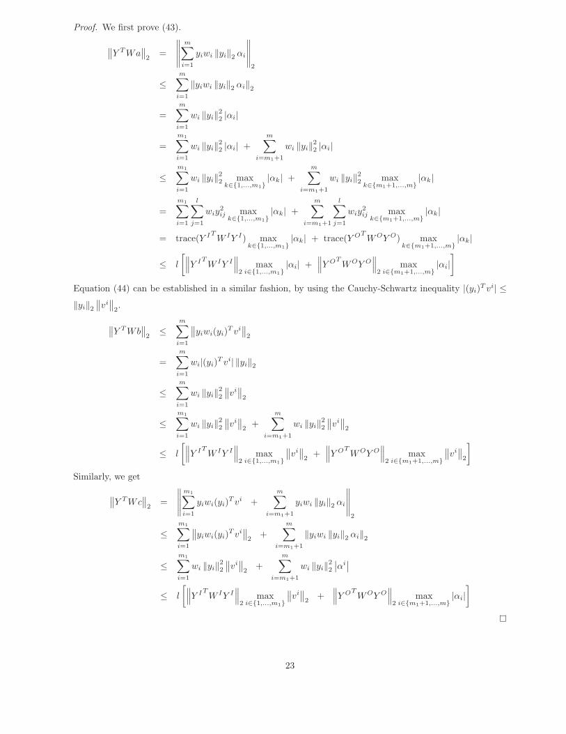
Proof. We first prove (43).

∥∥Y T Wa∥∥

2=

∥∥∥∥∥m∑

i=1

yiwi ‖yi‖2 αi

∥∥∥∥∥2

≤m∑

i=1

‖yiwi ‖yi‖2 αi‖2

=m∑

i=1

wi ‖yi‖22 |αi|

=m1∑i=1

wi ‖yi‖22 |αi| +m∑

i=m1+1

wi ‖yi‖22 |αi|

≤m1∑i=1

wi ‖yi‖22 maxk∈{1,...,m1}

|αk| +m∑

i=m1+1

wi ‖yi‖22 maxk∈{m1+1,...,m}

|αk|

=m1∑i=1

l∑j=1

wiy2ij max

k∈{1,...,m1}|αk| +

m∑i=m1+1

l∑j=1

wiy2ij max

k∈{m1+1,...,m}|αk|

= trace(Y ITW IY I) max

k∈{1,...,m1}|αk| + trace(Y OT

WOY O) maxk∈{m1+1,...,m}

|αk|

≤ l


∥∥∥2

maxi∈{1,...,m1}

|αi| +∥∥∥Y OT

WOY O∥∥∥

2max

i∈{m1+1,...,m}|αi|

]Equation (44) can be established in a similar fashion, by using the Cauchy-Schwartz inequality |(yi)T vi| ≤‖yi‖2

∥∥vi∥∥

2.

∥∥Y T Wb∥∥

2≤

m∑i=1

∥∥yiwi(yi)T vi∥∥

2

=m∑

i=1

wi|(yi)T vi| ‖yi‖2

≤m∑

i=1

wi ‖yi‖22∥∥vi

∥∥2

≤m1∑i=1


∥∥2

+m∑

i=m1+1


∥∥2

≤ l


∥∥∥2

maxi∈{1,...,m1}

∥∥vi∥∥

2+

∥∥∥Y OTWOY O

∥∥∥2

maxi∈{m1+1,...,m}

∥∥vi∥∥

2

]Similarly, we get

∥∥Y T Wc∥∥

2=

∥∥∥∥∥m1∑i=1

yiwi(yi)T vi +m∑

i=m1+1

yiwi ‖yi‖2 αi

∥∥∥∥∥2

≤m1∑i=1

∥∥yiwi(yi)T vi∥∥

2+

m∑i=m1+1

‖yiwi ‖yi‖2 αi‖2

≤m1∑i=1


∥∥2

+m∑

i=m1+1

wi ‖yi‖22∣∣αi∣∣

≤ l


∥∥∥2

maxi∈{1,...,m1}

∥∥vi∥∥

2+

∥∥∥Y OTWOY O

∥∥∥2

maxi∈{m1+1,...,m}

|αi|]

23

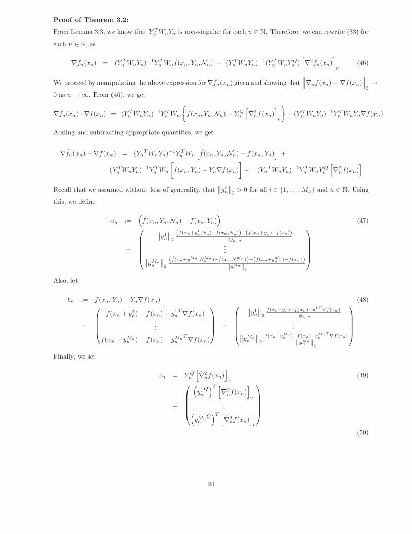
Proof of Theorem 3.2:

From Lemma 3.3, we know that Y Tn WnYn is non-singular for each n ∈ N. Therefore, we can rewrite (33) for

each n ∈ N, as

∇fn(xn) = (Y Tn WnYn)−1Y T

n Wnf(xn, Yn,Nn) − (Y Tn WnYn)−1(Y T

n WnY Qn )

[∇2fn(xn)

]v

(46)

We proceed by manipulating the above expression for∇fn(xn) given and showing that∥∥∥∇nf(xn)−∇f(xn)

∥∥∥2→

0 as n→∞. From (46), we get

∇fn(xn)−∇f(xn) = (Y Tn WnYn)−1Y T

n Wn

{f(xn, Yn,Nn)− Y Q

n

[∇2

nf(xn)]

v

}− (Y T

n WnYn)−1Y Tn WnYn∇f(xn)

Adding and subtracting appropriate quantities, we get

∇fn(xn)−∇f(xn) = (YnT WnYn)−1Y T

n Wn

[f(xn, Yn,Nn)− f(xn, Yn)

]+

(Y Tn WnYn)−1Y T

n Wn

[f(xn, Yn)− Yn∇f(xn)

]− (Yn

T WnYn)−1Y Tn WnY Q

n

[∇2

nf(xn)]

Recall that we assumed without loss of generality, that∥∥yi

n

∥∥2

> 0 for all i ∈ {1, . . . , Mn} and n ∈ N. Using

this, we define

an :=(f(xn, Yn,Nn)− f(xn, Yn)

)(47)

=

⎛⎜⎜⎜⎜⎝

∥∥y1n

∥∥2

(f(xn+y1n,N1

n)−f(xn,N1n))−(f(xn+y1

n)−f(xn))‖y1

n‖2...∥∥yMn

n

∥∥2

(f(xn+yMnn ,NMn

n )−f(xn,NMnn ))−(f(xn+yMn

n )−f(xn))‖yMn

n ‖2

⎞⎟⎟⎟⎟⎠

Also, let

bn := f(xn, Yn)− Yn∇f(xn) (48)

=

⎛⎜⎜⎜⎝

f(xn + y1n)− f(xn)− y1

nT∇f(xn)

...

f(xn + yMnn )− f(xn)− yMn

nT∇f(xn)

⎞⎟⎟⎟⎠ =

⎛⎜⎜⎜⎜⎝

∥∥y1n

∥∥2

f(xn+y1n)−f(xn)−y1

nT ∇f(xn)

‖yin‖2

...∥∥yMnn

∥∥2

f(xn+yMnn )−f(xn)−yMn

nT ∇f(xn)

‖yMnn ‖2

⎞⎟⎟⎟⎟⎠

Finally, we set

cn = Y Qn

[∇2

nf(xn)]

v(49)

=

⎛⎜⎜⎜⎜⎝(y1

nQ)T [∇2

nf(xn)]

v...(

yMnn

Q)T [∇2

nf(xn)]

v

⎞⎟⎟⎟⎟⎠

(50)

24

Using the notation in (19) and the fact that∥∥yi

n

∥∥2

> 0 for all i = 1, . . . , Mn and n ∈ N, we get

cn =

⎛⎜⎜⎜⎝

12y1

nt∇2

nf(xn)y1n

...12yMn

nt∇2

nf(xn)yMnn

⎞⎟⎟⎟⎠ =

⎛⎜⎜⎜⎜⎝

12

∥∥y1n

∥∥2

y1n

t∇2nf(xn)y1

n

‖y1n‖2

...12

∥∥yMnn

∥∥2

yMnn

t∇2nf(xn)yMn

n

‖yMnn ‖2

⎞⎟⎟⎟⎟⎠

Then, using the notation defined above, we get

∇nf(xn)−∇f(x) = (YnT WnYn)−1Y T

n Wnan + (YnT WnYn)−1Y T

n Wnbn − (Y Tn WnYn)−1Y T

n Wncn

Using the triangle inequality,

∥∥∥∇nf(xn)−∇f(x)∥∥∥

2≤

∥∥(YnT WnYn)−1Y T

n Wnan

∥∥2+∥∥(Yn

T WnYn)−1Y Tn Wnbn

∥∥2+∥∥(Y T

n WnYn)−1Y Tn Wncn

∥∥2

(51)

Let us consider the three terms on the right hand side of (51) in order.

Using (43) in Lemma 3.2, we get

∥∥(Y Tn WnYn)−1Y T

n Wnan

∥∥2≤


∥∥2

∥∥Y Tn Wnan

∥∥2

≤ l∥∥(Y T

n WnYn)−1∥∥

2

⎡⎣⎧⎨⎩∥∥∥Y I

n

TW I

nY In

∥∥∥2

maxi∈{1,...,MI

n}

∣∣∣(f(xn + yin, N i

n)− f(xn, N in))−(f(xn + yi

n)− f(xn))∣∣∣

‖yin‖2

⎫⎬⎭

+

⎧⎨⎩∥∥∥Y O

n

TWO

n Y On

∥∥∥2

maxi∈{MI

n+1,...,Mn}



n)− f(xn))∣∣∣

‖yin‖2

⎫⎬⎭⎤⎦ (52)

Now, we consider the two terms of (52) in order. First, from Lemma 3.3, we know that for all n ∈ N,∥∥(Y Tn WnYn)−1

∥∥2

∥∥∥Y In

TW I

nY In

∥∥∥2≤ KI

λ. From Assumption A 5, we know that

limn→∞ min

i=1,...,MIn

N in = ∞

Also, we know that {xn}n∈N⊂ C and xn + yi

n ∈ C for each i = 1, . . . ,Mn and n ∈ N. Now, from Assumption

A 4 and the definition of the norm on W0(C), we get for any ε > 0 there exists Nε ∈ N such that for all

N > Nε,

supx+y,x∈C

y �=0

∣∣∣(f(x + y,N)− f(x,N))− (f(x + y)− f(x))

∣∣∣‖y‖2

≤ ε

Also, from Assumption A 5, we know that there exists nε ∈ N such that for all n > nε, min{N in : i =

1, . . . ,M In} > Nε. Thus, we get combining these two facts, that for any ε > 0 , there exists nε ∈ N, such

that for all n > nε,

maxi∈{1,...,MI

n}



n)− f(xn))∣∣∣

‖yin‖2

≤ ε

25

Therefore,

limn→∞ max

i∈{1,...,MIn}



n)− f(xn))∣∣∣

‖yin‖2

= 0

Consequently, we get that,

limn→∞


∥∥2

∥∥∥Y In

TW I

nY In

∥∥∥2

maxi∈{1,...,MI

n}



n)− f(xn))∣∣∣

‖yin‖2

= 0

Next consider the second term on the right side of (52). First, from Lemma 3.3, we get

limn→∞


∥∥2

∥∥∥Y On

TWO

n Y On

∥∥∥2

= 0

Now, we note that for each n ∈ N,

maxi∈{MI

n+1,...,Mn}



n)− f(xn))∣∣∣

‖yin‖2

≤ maxi∈{MI

n+1,...,Mn}

{|f(xn + yi


n)|‖yi

n‖2+|f(xn + yi

n)− f(xn)|‖yi

n‖2

}

≤ maxi∈{MI

n+1,...,Mn}

⎧⎪⎨⎪⎩ sup

x,x+y∈Cy �=0

|f(x + y,N in)− f(x,N i

n)|‖y‖2

+ supx,x+y∈C

y �=0

|f(x + y)− f(x)|‖y‖2

⎫⎪⎬⎪⎭

≤ ‖f‖W0(C) + max

i∈{MIn+1,...,Mn}

∥∥∥f(·, N in)∥∥∥

W0(C)

From Assumption A 4, we know that

limN→∞

∥∥∥f(·, N)− f∥∥∥

W0(C)= 0

Hence, the sequence{∥∥∥f(·, N)W0(C)

∥∥∥}N∈N

is bounded and there exists Kf < ∞, such that ‖f‖W0(C) < Kf

and supN∈N

∥∥∥f(·, N)W0(C)

∥∥∥ < Kf where C ⊂ E is the compact set mentioned in Assumption A 7. Since we

also know from Assumption A 7 that xn ∈ C for each n ∈ N and xn + yin ∈ C for each n ∈ N, we get

maxi∈{MI

n+1,...,Mn}

∥∥∥f(·, N in)∥∥∥

W0(C)< Kf

Consequently , we get that

‖f‖W0(C) + max

i∈{MIn+1,...,Mn}

∥∥∥f(·, N in)∥∥∥

W0(C)≤ 2Kf

Hence, using the fact that limn→∞∥∥(Y T

n WnYn)−1∥∥

2

∥∥∥Y On

TWO

n Y On

∥∥∥2

= 0, we finally get

limn→∞


∥∥2

∥∥∥Y On

TWO

n Y On

∥∥∥2

maxi∈{MI

n+1,...,Mn}



n)− f(xn))∣∣∣

‖yin‖2

= 0

Thus, we have shown that

limn→∞

∥∥(Y Tn Yn)−1Y T

n an

∥∥2

= 0

26

Next, we consider the second term on the right side of (51). Using (43) in Lemma 3.4, we get


n Wnbn

∥∥2≤ l


∥∥2×[{∥∥∥Y I

n

TW I

nY In

∥∥∥2

maxi∈{1,...,MI

n}

∣∣∣∣∣f(xn + yin)− f(xn)− yi

nT∇f(xn)

‖yin‖2

∣∣∣∣∣}

+

{∥∥∥Y On

TWO

n Y On

∥∥∥2

maxi∈{MI

n+1,...,Mn}


nT∇f(xn)

‖yin‖2

∣∣∣∣∣}]

(53)

We will first show that

limn→∞ l


∥∥2

∥∥∥Y In

TW I

nY In

∥∥∥2

maxi∈{1,...,MI

n}


nT∇f(xn)

‖yin‖2

∣∣∣∣∣ = 0

From Assumption A 4, we know that ∇f : C −→ Rl is continuous on C. Since the set C ⊂ E (defined in

Assumption A 7) is compact, we get that ∇f is uniformly continuous on C. That is, for any ε > 0, there

exists δ > 0 such that

supx,x+y∈C0<‖y‖2≤δ

∣∣∣∣f(x + y)− f(x)−∇f(x)T y

‖y‖2

∣∣∣∣ < ε (54)

From Assumption A 7, we know that {xn}n∈N⊂ C and {xn + yi

n : i = 1, . . . ,Mn} ⊂ C for each n ∈ N.

Further, we know from Assumption A 6 that δn → 0 as n→∞. Since∥∥yi

n

∥∥2≤ δn and 0 ≤ tin ≤ 1 for each

i = 1, . . . , M In and each n ∈ N, we get that

limn→∞ max

i∈{1,...,MIn}

∥∥xn + yin − xn

∥∥2

= limn→∞ max

i∈{1,...,MIn}

∥∥yin

∥∥2

= 0 (55)

It follows from (55) that given any δ > 0, there exists an n1 ∈ N such that∥∥xn + yi

n − xn

∥∥2

< δ for all

i ∈ {1, . . . , M In} and n > n1. Therefore, using (54), we get that for any ε > 0, there exists n1 ∈ N, such that∣∣∣∣∣f(xn + yi

n)− f(xn)− yin

T∇f(xn)‖yi

n‖2

∣∣∣∣∣ < ε for all i = 1, . . . ,M In and n > n1

Thus

limn→∞ max

i∈{1,...,MIn}


nT∇f(xn)

‖yin‖2

∣∣∣∣∣ = 0

Now, using (38) in Lemma 3.3, we get

limn→∞ l


∥∥2

∥∥∥Y In

TW I

nY In

∥∥∥2

maxi∈{1,...,MI

n}


nT∇f(xn)

‖yin‖2

∣∣∣∣∣ ≤l KI

λ limn→∞ max

i∈{1,...,MIn}


nT∇f(xn)

‖yin‖2

∣∣∣∣∣ = 0

Hence, the first term on the right side of (53) converges to zero. Next we show that

limn→∞ l


∥∥2

∥∥∥Y On

TWO

n Y On

∥∥∥2

maxi∈{MI

n+1,...,Mn}


nT∇f(xn)

‖yin‖2

∣∣∣∣∣ = 0

27

Again, since f is continuously differentiable on C and C ⊂ E is compact, we get from Lemma 2.2 in ?, that

there exists K1f <∞ such that

supx+y,x∈C

y �=0

∣∣∣∣f(x + y)− f(x)− yT∇f(x)‖y‖2

∣∣∣∣ < K1f

Since we know from Assumption A 7 that xn ∈ C for each n ∈ N and xn + yin ∈ C for each n ∈ N and

i ∈ {1, . . . , Mn}, we get that for each n ∈ N

maxi∈{MI

n+1,...,Mn}


nT∇f(xn)

‖yin‖2

∣∣∣∣∣ ≤ K1f

Now, using (39) in Lemma 3.3, we get

limn→∞ l


∥∥2

∥∥∥Y On

TWO

n Y On

∥∥∥2

maxi∈{MI

n+1,...,Mn}


nT∇f(xn)

‖yin‖2

∣∣∣∣∣ ≤2l K1f lim

n→∞∥∥(Y T

n WnYn)−1∥∥

2

∥∥∥Y On

TWO

n Y On

∥∥∥2

= 0

Thus, the second term on the right side of (53) converges to zero. Hence∥∥(Y T

n WnYn)−1Y Tn Wnbn

∥∥2→ 0 as

n→∞.

Finally, consider the third term on the right in (51). Again using (43),


n Wncn

∥∥2≤ l

2


∥∥2

⎡⎣⎧⎨⎩∥∥∥Y I

n

TW I

nY In

∥∥∥2

maxi∈{1,...,MI

n}

∣∣∣yin

T∇2fn(xn)yin

∣∣∣‖yi

n‖2

⎫⎬⎭

+

⎧⎨⎩∥∥∥Y O

n

TWO

n Y On

∥∥∥2

maxi∈{MI

n+1,...,Mn}

∣∣∣yin

T∇2fn(xn)yin

∣∣∣‖yi

n‖2

⎫⎬⎭⎤⎦

Since ∇2fn(xn) ∈ Sl×l is a symmetric matrix, it is well known that

∣∣∣yin

T∇2fn(xn)yin

∣∣∣ ≤ ∥∥∥∇2fn(xn)∥∥∥

2

∥∥yin

∥∥2

2

for each n ∈ N and i ∈ {1, . . . ,Mn}. Using∥∥yi

n

∥∥2

> 0 for each i = 1, . . . ,Mn and n ∈ N, we get∣∣∣yin

T∇2fn(xn)yin

∣∣∣‖yi

n‖2≤

∥∥∥∇2fn(xn)∥∥∥

2

∥∥yin

∥∥2

2

‖yin‖2

=∥∥∥∇2fn(xn)

∥∥∥2

∥∥yin

∥∥2

Now, from Assumption A 8 we know∥∥∥∇2fn(xn)

∥∥∥2≤ KH for all n ∈ N. Hence,


n Wncn

∥∥2≤ lKH

2


∥∥2

[{∥∥∥Y In

TW I

nY In

∥∥∥2

maxi∈{1,...,MI

n}

∥∥yin

∥∥2

}

+{∥∥∥Y O

n

TWO

n Y On

∥∥∥2

maxi∈{MI

n+1,...,Mn}

∥∥yin

∥∥2

}](56)

28

But we know from Assumption A 6, that maxi∈{1,...,MIn}∥∥yi

n

∥∥2→ 0 as n → ∞. Therefore, using (38) in

Lemma 3.3, we get

limn→∞

(lKH

2

)∥∥(Y Tn WnYn)−1

∥∥2

∥∥∥Y In

TW I

nY In

∥∥∥2

maxi∈{1,...,MI

n}

∥∥yin

∥∥2≤(

lKHKIλ

2

)lim

n→∞ maxi∈{1,...,MI

n}

∥∥yin

∥∥2

= 0

Now, we know from Assumption A 7, that {xn}n∈N⊂ C and xn + yi

n ⊂ C for all i ∈ {M In + 1, . . . , Mn} and

n ∈ N, where C ⊂ E is compact. Therefore, there must exist Ky <∞ such that maxi∈{MIn+1,...,Mn}

∥∥yin

∥∥2

<

Ky for all n ∈ N. Thus, using (39) in Lemma 3.3 we get

limn→∞

(lKH

2

)∥∥(Y Tn WnYn)−1

∥∥2

∥∥∥Y On

TWO

n Y On

∥∥∥2

maxi∈{1,...,MI

n}

∥∥yin

∥∥2≤(

lKHKy

2

)lim

n→∞∥∥(Y T

n WnYn)−1∥∥

2

∥∥∥Y On

TWO

n Y On

∥∥∥2

= 0

Therefore∥∥(Y T

n WnYn)−1Y Tn Wncn

∥∥2→∞ as n→∞. Hence we have shown that,

limn→∞

∥∥∥∇nf(xn)−∇f(xn)∥∥∥

2= 0

In particular, if xn → x ∈ X as n→∞, then we get from the continuous differentiability of f that

limn→∞

∥∥∥∇nf(xn)−∇f(x)∥∥∥

2≤ lim

n→∞

∥∥∥∇nf(xn)−∇f(xn)∥∥∥

2+ lim

n→∞ ‖∇f(xn)−∇f(x)‖2 = 0

�

Corollary 3.5. Consider any sequence {xn}n∈N⊂ X and let all the assumptions of Theorem 3.2 hold.

Suppose for each n ∈ N, ∇nf(xn) ∈ Rl and ∇2

nf(xn) ∈ Sl×l are picked to satisfy (25). Then,

limn→∞

∥∥∥∇nf(xn)−∇f(xn)∥∥∥

2= 0

Proof. The result follows from the fact that if ∇nf(xn) and ∇2nf(xn) satisfy (25) for each n ∈ N, then they

also automatically satisfy (33).

Corollary 3.6. Consider any sequence {xn}n∈N⊂ X and let all the assumptions of Theorem 3.2 hold.

Suppose for each n ∈ N, ∇nf(xn) ∈ Rl is picked such that

(Y Tn Wn)Yn ∇nf(xn) = Y T

n Wnf(xn, Yn,Nn)

Then we have,

limn→∞

∥∥∥∇nf(xn)−∇f(xn)∥∥∥

2= 0

Proof. The required result follows from Theorem 3.2 when we set ∇2nf(xn) = 0 in (33), for each n ∈ N.

29

Next, we present some stronger conditions that ensure the convergence of both the gradient and Hessian

approximations.

Theorem 3.7. Consider a sequence {xn}n∈N⊂ X and let for each n ∈ N, ∇nf(xn) ∈ R


l×l

be picked so as to satisfy (25). Suppose that the following assumptions hold.

A 9. For any compact set D ⊂ E, we get f ∈ C2(D),{

f(·, N)}

N∈N

⊂W1(D) and

limn→∞

∥∥∥f(·, N)− f∥∥∥

W1(D)= 0

A 10. There exists a sequence{N#

n

}n∈N

of sample sizes such that

1. N in = N#

n for all i = 1, . . . ,Mn and

2. N#n →∞ as n→∞.

A 11. The set of design points{xn + yi

n : i = 1, . . . ,Mn and n ∈ N}

and the sequence {Wn}n∈Nof weight

matrices, satisfy the following.

1. There exists a compact set C ⊂ E such that the point xn and the set of design points {xn + yin : i =

1, . . . , Mn} satisfy

xn ∈ C and {xn + yin : i = 1, . . . ,Mn} ⊂ C (57)

for each n ∈ N.

2. There exists KIλ <∞ such that for each n ∈ N∥∥∥(ZI

n)T W In ZI

n

∥∥∥2

∥∥∥((ZIn)T W I

n ZIn)−1

∥∥∥2

< KIλ (58)

3.

limn→∞

∥∥∥(ZOn )T WO

n ZOn

∥∥∥2∥∥∥(ZI

n)T W In ZI

n

∥∥∥2

= 0 (59)

Further, let Assumption A 6 also hold. Then, we have,

limn→∞

∥∥∥∇nf(xn)−∇f(xn)∥∥∥

2= 0 and lim

n→∞

∥∥∥∇2nf(xn)−∇2f(xn)

∥∥∥2

= 0

In particular, if {xn}n∈N⊂ X is such that xn → x ∈ X as n→∞, then

limn→∞ ∇nf(xn) = ∇f(x) and lim

n→∞ ∇2nf(xn) = ∇2f(x)

Before proving Theorem 3.7, we state and prove a useful lemma.

Lemma 3.8. Let Assumption A 11 hold. Then, ZTn WnZn and ZT

n WnZn are positive definite for each n ∈ N

and the following hold true.

30

1. ∥∥∥(ZTn WnZn)−1

∥∥∥2

∥∥∥(ZIn)T W I

n ZIn

∥∥∥2


2.

limn→∞

∥∥∥(ZTn WnZn)−1

∥∥∥2

∥∥∥(ZOn )T WO

n ZOn

∥∥∥2

= 0 (61)

Proof. Since (ZIn)T W I

n ZIn is a symmetric and positive semidefinite matrix, we get from (58) that

λmin((ZIn)T W I

n ZIn) =

1∥∥∥((ZIn)T W I

n ZIn)−1

∥∥∥2

> 0

Further, it is easily seen that

ZTn WnZn = (ZI

n)T W In ZI

n + (ZOn )T WO

n ZOn

Now, since (ZOn )T WO

n ZOn is positive semidefinite, from the interlocking eigenvalues theorem, we know that

λmin(ZTn WnZn) ≥ λmin((ZI

n)T W In ZI

n) > 0

Therefore , ZTn WnZn is positive definite. Further, from the definition of Dn in (32), we know that Dn is

positive definite for each n ∈ N. Since the product of positive definite matrices remains positive definite, we

get that ZTn WnZn = D−1

n (ZTn WnZn)D−1

n is positive definite for each n ∈ N. Now,∥∥∥(ZTn WnZn)−1

∥∥∥2

=1

λmin(ZTn WnZn)

≤ 1λmin((ZI

n)T W In ZI

n)=


n ZIn)−1

∥∥∥2

(62)

Therefore, we see that for any n ∈ N, using (62),∥∥∥(ZTn WnZn)−1

∥∥∥2

∥∥∥(ZIn)T W I

n ZIn

∥∥∥2≤


n ZIn)−1

∥∥∥2

∥∥∥(ZIn)T W I

n ZIn

∥∥∥2≤ KI

λ

Thus, we have shown that (60) holds. Similarly,


∥∥∥2

∥∥∥(ZOn )T WO

n ZOn

∥∥∥2≤


∥∥∥2

∥∥∥(ZIn)T W I

n ZIn

∥∥∥2

⎛⎝∥∥∥(ZO

n )T WOn ZO

n

∥∥∥2∥∥∥(ZI

n)T W In ZI

n

∥∥∥2

⎞⎠

Using (60) on the right hand side of the above equation, we get


∥∥∥2

∥∥∥(ZOn )T WO

n ZOn

∥∥∥2≤ KI

λ

⎛⎝∥∥∥(ZO

n )T WOn ZO

n

∥∥∥2∥∥∥(ZI

n)T W In ZI

n

∥∥∥2

⎞⎠

Finally, we use (37) in Assumption A 11 to get that

limn→∞


∥∥∥2

∥∥∥(ZOn )T WO

n ZOn

∥∥∥2≤ KI

λ limn→∞

∥∥∥(ZOn )T WO

n ZOn

∥∥∥2∥∥∥(ZI

n)T W In ZI

n

∥∥∥2

= 0

31

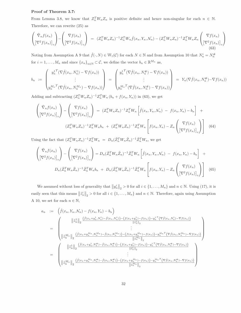
Proof of Theorem 3.7:

From Lemma 3.8, we know that ZTn WnZn is positive definite and hence non-singular for each n ∈ N.

Therefore, we can rewrite (25) as⎛⎝ ∇nf(xn)[∇2f(xn)

]v

⎞⎠−

⎛⎝ ∇f(xn)[∇2f(xn)

]v

⎞⎠ = (ZT

n WnZn)−1ZTn Wnf(xn, Yn,Nn)− (ZT

n WnZn)−1ZTn WnZn

⎛⎝ ∇f(xn)[∇2f(xn)

]v

⎞⎠

(63)

Noting from Assumption A 9 that f(·, N) ∈W1(C) for each N ∈ N and from Assumption 10 that N in = N#

n

for i = 1, . . . ,Mn and since {xn}n∈N⊂ C, we define the vector bn ∈ R

Mn as,

bn :=

⎛⎜⎜⎜⎝

y1n

T (∇f(xn, N1n)−∇f(xn))...

yMnn

T (∇f(xn, NMnn )−∇f(xn))

⎞⎟⎟⎟⎠ =

⎛⎜⎜⎜⎝

y1n

T (∇f(xn, N#n )−∇f(xn))...

yMnn

T (∇f(xn, N#n )−∇f(xn))

⎞⎟⎟⎟⎠ = Yn(∇f(xn, N#

n )−∇f(xn))

Adding and subtracting (ZTn WnZn)−1ZT

n Wn (bn + f(xn, Yn)) in (63), we get⎛⎝ ∇nf(xn)[∇2f(xn)

]v

⎞⎠−

⎛⎝ ∇f(xn)[∇2f(xn)

]v

⎞⎠ = (ZT

n WnZn)−1ZTn Wn

[f(xn, Yn,Nn) − f(xn, Yn)− bn

]+

(ZTn WnZn)−1ZT

n Wnbn + (ZTn WnZn)−1ZT

n Wn

⎡⎣f(xn, Yn)− Zn

⎛⎝ ∇f(xn)[∇2f(xn)

]v

⎞⎠⎤⎦ (64)

Using the fact that (ZTn WnZn)−1ZT

n Wn = Dn(ZTn WnZn)−1ZT

n Wn, we get⎛⎝ ∇nf(xn)[∇2f(xn)

]v

⎞⎠−

⎛⎝ ∇f(xn)[∇2f(xn)

]v

⎞⎠ = Dn(ZT

n WnZn)−1ZTn Wn

[f(xn, Yn,Nn) − f(xn, Yn)− bn

]+

Dn(ZTn WnZn)−1ZT

n Wnbn + Dn(ZTn WnZn)−1ZT

n Wn

⎡⎣f(xn, Yn)− Zn

⎛⎝ ∇f(xn)[∇2f(xn)

]v

⎞⎠⎤⎦ (65)

We assumed without loss of generality that∥∥yi

n

∥∥2

> 0 for all i ∈ {1, . . . , Mn} and n ∈ N. Using (17), it is

easily seen that this means∥∥zi

n

∥∥2

> 0 for all i ∈ {1, . . . ,Mn} and n ∈ N. Therefore, again using Assumption

A 10, we set for each n ∈ N,

an :=(f(xn, Yn,Nn)− f(xn, Yn)− bn

)

=

⎛⎜⎜⎜⎜⎝

∥∥z1n

∥∥2

(f(xn+y1n,N1

n)−f(xn,N1n))−(f(xn+y1

n)−f(xn))−y1n

T (∇f(xn,N1n)−∇f(xn))

‖z1n‖2

...∥∥zMnn

∥∥2

(f(xn+yMnn ,NMn

n )−f(xn,NMnn ))−(f(xn+yMn

n )−f(xn))−yMnn

T (∇f(xn,NMnn )−∇f(xn))

‖zMnn ‖2

⎞⎟⎟⎟⎟⎠

=

⎛⎜⎜⎜⎜⎝

∥∥z1n

∥∥2

(f(xn+y1n,N#

n )−f(xn,N#n ))−(f(xn+y1

n)−f(xn))−y1n

T (∇f(xn,N#n )−∇f(xn))

‖z1n‖2

...∥∥zMnn

∥∥2

(f(xn+yMnn ,N#

n )−f(xn,N#n ))−(f(xn+yMn

n )−f(xn))−yMnn

T (∇f(xn,N#n )−∇f(xn))

‖zMnn ‖2

⎞⎟⎟⎟⎟⎠

32

Let us simplify the third term on the right side of (65).

f(xn, Yn)− Zn

⎛⎝ ∇f(xn)[∇2f(xn)

]v

⎞⎠ = f(xn, Yn)− Yn∇f(xn) − Y Q

n ∇2nf(xn)

=

⎛⎜⎜⎜⎝


nT∇f(xn)− (y1

nQ)T

[∇2f(xn)

]v

...


nT∇f(xn)− (yMn

nQ)T

[∇2f(xn)

]v

⎞⎟⎟⎟⎠

=

⎛⎜⎜⎜⎝


nT∇f(xn)− 1

2

(y1

nT∇2f(xn)y1

n

)...


nT∇f(xn)− 1

2

(yMn

nT∇2f(xn)yMn

n

)⎞⎟⎟⎟⎠

Again noting that δn > 0 for each n ∈ N and∥∥zi

n

∥∥2

> 0 for each i ∈ {1, . . . , Mn} and n ∈ N, we set

cn := f(x, Yn)− Zn

⎛⎝ ∇f(xn)[∇2f(xn)

]v

⎞⎠

=

⎛⎜⎜⎜⎜⎝

∥∥z1n

∥∥2

f(xn+y1n)−f(xn)−y1

nT ∇f(xn)− 1

2 (y1n

T ∇2f(xn)y1n)

‖z1n‖2

...∥∥zMnn

∥∥2

f(xn+yMnn )−f(xn)−yMn

nT ∇f(xn)− 1

2

“yMn

nT ∇2f(xn)yMn

n

”

‖zMnn ‖2

⎞⎟⎟⎟⎟⎠

Therefore, we finally have for each n ∈ N,⎛⎝ ∇nf(xn)[∇2f(xn)

]v

⎞⎠−

⎛⎝ ∇f(xn)[∇2f(xn)

]v

⎞⎠ = Dn(ZT

n WnZn)−1ZTn Wnan + Dn(ZT

n WnZn)−1ZTn Wnbn +

Dn(ZTn WnZn)−1ZT

n Wncn

⇒

∥∥∥∥∥∥⎛⎝ ∇nf(xn)[∇2f(xn)

]v

⎞⎠−

⎛⎝ ∇f(xn)[∇2f(xn)

]v

⎞⎠∥∥∥∥∥∥

2

≤∥∥∥Dn(ZT

n WnZn)−1ZTn Wnan

∥∥∥2

+∥∥∥Dn(ZT

n WnZn)−1ZTn Wnbn

∥∥∥2

+∥∥∥Dn(ZT

n WnZn)−1ZTn Wncn

∥∥∥2

(66)

Next, we show that all three terms on the right side of (66) converge to zero as n → ∞. But first,

we note that from Assumption A 6, δn → 0 as n → ∞. Therefore, there exists n∗ ∈ N, such that for all

n > n∗, δn < 1. This means that for all n > n∗, (1/δn)2 > (1/δn). Therefore, we get that for all n > n∗,

‖Dn‖2 = (1/δn)2.

Let us consider the first term right side of (66) for n > n∗. First, we note that

∥∥∥Dn(ZTn WnZn)−1ZT

n Wnan

∥∥∥2≤ ‖Dn‖2


∥∥∥2

∥∥∥ZTn Wnan

∥∥∥2

=(

1δ2n

) ∥∥∥(ZTn WnZn)−1

∥∥∥2

∥∥∥ZTn Wnan

∥∥∥2

33

Recall that the matrix Zn has p = l + l(l + 1)/2 columns. Using this fact in (43) of Lemma 3.4, we get


n Wnan

∥∥∥2≤ p


∥∥∥2×

⎡⎣⎧⎨⎩∥∥∥(ZI

n)T W In ZI

n

∥∥∥2×

maxi∈{1,...,MI

n}

∣∣∣∣∣∣(f(xn + yi

n, N#n )− f(xn, N#

n ))−(f(xn + yi

n)− f(xn))− yi

nT(∇f(xn, N#

n )−∇f(xn))

δ2n ‖zi

n‖2

∣∣∣∣∣∣⎫⎬⎭

+

⎧⎨⎩∥∥∥(ZO

n )T WOn ZO

n

∥∥∥2×

maxi∈{MI

n+1,...,Mn}

∣∣∣∣∣∣(f(xn + yi

n, N#n )− f(xn, N#

n ))−(f(xn + yi

n)− f(xn))− yi

nT(∇f(xn, N#

n )−∇f(xn))

δ2n ‖zi

n‖2

∣∣∣∣∣∣⎫⎬⎭⎤⎦

From the above, we get∥∥∥Dn(ZTn WnZn)−1ZT

n Wnan

∥∥∥2≤ p


∥∥∥2

(∥∥∥(ZIn)T W I

n ZIn

∥∥∥2

+∥∥∥(ZO

n )T WOn ZO

n

∥∥∥2

)×

maxi∈{1,...,Mn}

∣∣∣∣∣∣(f(xn + yi

n, N#n )− f(xn, N#

n ))−(f(xn + yi

n)− f(xn))− yi

nT(∇f(xn, N#

n )−∇f(xn))

δ2n ‖zi

n‖2

∣∣∣∣∣∣First, from Assumption A 11 and Lemma 3.8 we get that∥∥∥(ZT

n WnZn)−1∥∥∥

2

∥∥∥(ZIn)T W I

n ZIn

∥∥∥2≤ KI

λ for all n ∈ N

and

limn→∞


∥∥∥2

∥∥∥(ZOn )T WO

n ZOn

∥∥∥2

= 0

Therefore, clearly there exists a constant Kλ <∞ such that for all n ∈ N,∥∥∥(ZTn WnZn)−1

∥∥∥2

(∥∥∥(ZIn)T W I

n ZIn

∥∥∥2

+∥∥∥(ZO

n )T WOn ZO

n

∥∥∥2

)< Kλ (67)

Next, we note that from (17), for any n ∈ N and i ∈ {1, . . . , Mn},

δ2n

∥∥zin

∥∥2

=

√δ2n ‖yi

n‖22 +

(12

)‖yi

n‖42 ≥

(√12

)∥∥yin

∥∥2

2(68)

Therefore, for each i = 1, . . . ,Mn,∣∣∣∣∣∣(f(xn + yi

n, N#n )− f(xn, N#

n ))−(f(xn + yi

n)− f(xn))− yi

nT(∇f(xn, N#

n )−∇f(xn))

δ2n ‖zi

n‖2

∣∣∣∣∣∣ ≤√

2

∣∣∣∣∣∣(f(xn + yi

n, N#n )− f(xn, N#

n ))−(f(xn + yi

n)− f(xn))− yi

nT(∇f(xn, N#

n )−∇f(xn))

‖yin‖

22

∣∣∣∣∣∣Now from Assumption A 10, we know that, N#

n → ∞ as n → ∞. From Assumption A 9 we then get

that

limn→∞

∥∥∥f(·, N#n )− f

∥∥∥W1(C)

= 0

34

where C ⊂ E is the compact set defined in Assumption A 11. Therefore, we get from Lemma 2.4 in ? that

limn→∞ sup

x,x+y⊂Cy �=0

∣∣∣∣∣ (f(x + y,N#n )− f(x + y))− (f(x,N#

n )− f(x))− yT (∇f(x,N#n )−∇f(x))

‖y‖22

∣∣∣∣∣ = 0

Further, from Assumption A 11, we know that xn+yin ∈ C for each i = 1, . . . , Mn and n ∈ N and {xn}n∈N

⊂ C.Therefore, for each n ∈ N,

maxi∈{1,...,Mn}

∣∣∣∣∣∣(f(xn + yi

n, N#n )− f(xn, N#

n ))−(f(xn + yi

n)− f(xn))− yi

nT(∇f(xn, N#

n )−∇f(xn))

‖yin‖

22

∣∣∣∣∣∣ ≤sup

x,x+y⊂Cy �=0

∣∣∣∣∣ (f(x + y,N#n )− f(x + y))− (f(x,N#

n )− f(x))− yT (∇f(x,N#n )−∇f(x))

‖y‖22

∣∣∣∣∣Therefore, we get that

limn→∞ max

i∈{1,...,Mn}

∣∣∣∣∣∣(f(xn + yi

n, N#n )− f(xn, N#

n ))−(f(xn + yi

n)− f(xn))− yi

nT(∇f(xn, N#

n )−∇f(xn))

‖yin‖

22

∣∣∣∣∣∣ = 0

And hence we finally get

limn→∞


n Wnan

∥∥∥2≤√

2 p Kλ ×

limn→∞ max

i∈{1,...,Mn}

∣∣∣∣∣∣(f(xn + yi

n, N#n )− f(xn, N#

n ))−(f(xn + yi

n)− f(xn))− yi

nT(∇f(xn, N#

n )−∇f(xn))

‖yin‖

22

∣∣∣∣∣∣ = 0

Next, let us consider the second term on the right side of (66). Letting 0l(l+1)/2 denote a column vector

with l(l + 1)/2 elements each of which is equal to zero, it is easily seen that

bn = Yn(∇f(xn, N#n )−∇f(xn)) = Zn

⎛⎝∇f(xn, N#

n )−∇f(xn)

0l(l+1)/2

⎞⎠ = ZnD−1

n

⎛⎝∇f(xn, N#

n )−∇f(xn)

0l(l+1)/2

⎞⎠

Using the definition of bn, we get for each n ∈ N


n Wnbn

∥∥∥2

=

∥∥∥∥∥∥Dn(ZTn WnZn)−1ZT

n WnZnD−1n

⎛⎝∇f(xn, N#

n )−∇f(xn)

0l(l+1)/2

⎞⎠∥∥∥∥∥∥

2

=∥∥∥∇f(xn, N#

n )−∇f(xn)∥∥∥

2

From Assumption A 9 and the fact that C ⊂ E is compact, we know that∥∥∥f(·, N)− f

∥∥∥W1(C)

→ 0 as N →∞.

Since N#n → ∞ as n → ∞, we get that

∥∥∥f(·, N#n )− f

∥∥∥W1(C)

→ 0 as n → ∞. Further, using the fact that

{xn}n∈N⊂ C and the definition of the norm on W1(C), we get that

limn→∞

∥∥∥∇f(xn, N#n )−∇f(xn)

∥∥∥2

= 0

35

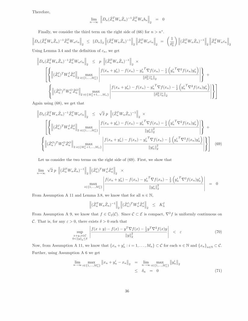
Therefore,

limn→∞


n Wnbn

∥∥∥2

= 0

Finally, we consider the third term on the right side of (66) for n > n∗.∥∥∥Dn(ZTn WnZn)−1ZT

n Wncn

∥∥∥2≤ ‖Dn‖2


∥∥∥2

∥∥∥ZTn Wncn

∥∥∥2

=(

1δ2n

)∥∥∥(ZTn WnZn)−1

∥∥∥2

∥∥∥ZTn Wncn

∥∥∥2

Using Lemma 3.4 and the definition of cn, we get∥∥∥Dn(ZTn WnZn)−1ZT

n Wncn

∥∥∥2≤ p


∥∥∥2×⎡

⎣⎧⎨⎩∥∥∥(ZI

n)T W In ZI

n

∥∥∥2

maxi∈{1,...,MI

n}

∣∣∣∣∣∣f(xn + yi

n)− f(xn)− yin

T∇f(xn)− 12

(yi

nT∇2f(xn)yi

n

)‖δ2

nzin‖2

∣∣∣∣∣∣⎫⎬⎭ +

⎧⎨⎩∥∥∥(ZO

n )T WOn ZO

n

∥∥∥2

maxi∈{MI

n+1,...,Mn}

∣∣∣∣∣∣f(xn + yi

n)− f(xn)− yin

T∇f(xn)− 12

(yi

nT∇2f(xn)yi

n

)‖δ2

nzin‖2

∣∣∣∣∣∣⎫⎬⎭⎤⎦

Again using (68), we get that∥∥∥Dn(ZTn WnZn)−1ZT

n Wncn

∥∥∥2≤√

2 p∥∥∥(ZT

n WnZn)−1∥∥∥

2×⎡

⎣⎧⎨⎩∥∥∥(ZI

n)T W In ZI

n

∥∥∥2

maxi∈{1,...,MI

n}

∣∣∣∣∣∣f(xn + yi

n)− f(xn)− yin

T∇f(xn)− 12

(yi

nT∇2f(xn)yi

n

)‖yi

n‖22

∣∣∣∣∣∣⎫⎬⎭ +

⎧⎨⎩∥∥∥(ZO

n )T WOn ZO

n

∥∥∥2

maxi∈{MI

n+1,...,Mn}

∣∣∣∣∣∣f(xn + yi

n)− f(xn)− yin

T∇f(xn)− 12

(yi

nT∇2f(xn)yi

n

)‖yi

n‖22

∣∣∣∣∣∣⎫⎬⎭⎤⎦ (69)

Let us consider the two terms on the right side of (69). First, we show that

limn→∞

√2 p


∥∥∥2

∥∥∥(ZIn)T W I

n ZIn

∥∥∥2×

maxi∈{1,...,MI

n}

∣∣∣∣∣∣f(xn + yi

n)− f(xn)− yin

T∇f(xn)− 12

(yi

nT∇2f(xn)yi

n

)‖yi

n‖22

∣∣∣∣∣∣ = 0

From Assumption A 11 and Lemma 3.8, we know that for all n ∈ N,∥∥∥(ZTn WnZn)−1

∥∥∥2

∥∥∥(ZIn)T W I

n ZIn

∥∥∥2≤ KI

λ

From Assumption A 9, we know that f ∈ C2(C). Since C ⊂ E is compact, ∇2f is uniformly continuous on

C. That is, for any ε > 0, there exists δ > 0 such that

supx+y,x∈C0<‖y‖2≤δ

∣∣∣∣∣f(x + y)− f(x)− yT∇f(x)− 12yT∇2f(x)y

‖y‖22

∣∣∣∣∣ < ε (70)

Now, from Assumption A 11, we know that {xn + yin : i = 1, . . . , Mn} ⊂ C for each n ∈ N and {xn}n∈N

⊂ C.Further, using Assumption A 6 we get

limn→∞ max

i∈{1,...,MIn}

∥∥xn + yin − xn

∥∥2

= limn→∞ max

i∈{1,...,MIn}

∥∥yin

∥∥2

≤ δn = 0 (71)

36

It follows that for any δ > 0, there exists an n > n∗ with such that for all n > n, δn < δ. Thus, 0 <∥∥yi

n

∥∥2≤ δ

for all i = 1, . . . ,M In and n > n. Thus, we get from (70) that for any ε > 0, there exists n ∈ N such that∣∣∣∣∣∣

f(xn + yin)− f(xn)− yi

nT∇f(xn)− 1

2

(yi

nT∇2f(xn)yi

n

)‖yi

n‖22

∣∣∣∣∣∣ < ε

for i ∈ {1, . . . ,M In} and n > n. Consequently,

limn→∞ max

i∈{1,...,MIn}

∣∣∣∣∣∣f(xn + yi

n)− f(xn)− yin

T∇f(xn)− 12

(yi

nT∇2f(xn)yi

n

)‖yi

n‖22

∣∣∣∣∣∣ = 0

Therefore, we see that

limn→∞

√2 p


∥∥∥2

∥∥∥(ZIn)T W I

n ZIn

∥∥∥2

maxi∈{1,...,MI

n}

∣∣∣∣∣∣f(xn + yi

n)− f(xn)− yin

T∇f(xn)− 12

(yi

nT∇2f(xn)yi

n

)‖yi

n‖22

∣∣∣∣∣∣≤√

2 p KIλ lim

n→∞ maxi∈{1,...,MI

n}

∣∣∣∣∣∣f(xn + yi

n)− f(xn)− yin

T∇f(xn)− 12

(yi

nT∇2f(xn)yi

n

)‖yi

n‖22

∣∣∣∣∣∣ = 0

Finally, we show that

limn→∞

√2 p


∥∥∥2

∥∥∥(ZOn )T WO

n ZOn

∥∥∥2×

maxi∈{MI

n+1,...,Mn}

∣∣∣∣∣∣f(xn + yi

n)− f(xn)− yin

T∇f(xn)− 12

(yi

nT∇2f(xn)yi

n

)‖yi

n‖22

∣∣∣∣∣∣ = 0

As we noted earlier, we get from Assumption A 9, f is twice continuously differentiable on C. Further, since

C is compact, we get from Lemma 2.3 in ? that there exists K2f <∞ such that

supx,x+y∈C

y �=0

∣∣f(x + y)− f(x)− yT∇f(x)−(

12

)yT∇2f(x)y

∣∣‖y‖22

< K2f

Since {xn + yin : i = 1, . . . , Mn} ⊂ C for each n ∈ N and {xn}n∈N

⊂ C, it follows that

maxi∈{MI

n+1,...,Mn}

∣∣∣∣∣∣f(xn + yi

n)− f(xn)− yin

T∇f(xn)− 12

(yi

nT∇2f(xn)yi

n

)‖yi

n‖22

∣∣∣∣∣∣ ≤ K2f

Also, from Assumption A 11 and Lemma 3.8, we get that

limn→∞


∥∥∥2

∥∥∥(ZOn )T WO

n ZOn

∥∥∥2

= 0

Therefore, we finally get

limn→∞

√2 p


∥∥∥2

∥∥∥(ZOn )T WO

n ZOn

∥∥∥2×

maxi∈{MI

n+1,...,Mn}

∣∣∣∣∣∣f(xn + yi

n)− f(xn)− yin

T∇f(xn)− 12

(yi

nT∇2f(xn)yi

n

)‖yi

n‖22

∣∣∣∣∣∣ ≤√

2 p K2f limn→∞


∥∥∥2

∥∥∥(ZOn )T WO

n ZOn

∥∥∥2

= 0

37

Thus, we have shown that∥∥∥Dn(ZT

n WnZn)−1ZTn Wncn

∥∥∥2→ 0 as n→∞. Hence it holds that

limn→∞

∥∥∥∥∥∥⎛⎝ ∇nf(xn)[∇2

nf(xn)]

v

⎞⎠−

⎛⎝ ∇f(xn)[∇2f(xn)

]v

⎞⎠∥∥∥∥∥∥

2

= 0

This in turn gives us

limn→∞

∥∥∥∇nf(xn)−∇f(xn)∥∥∥

2= 0 and lim

n→∞

∥∥∥∇2nf(xn)−∇2f(xn)

∥∥∥2

= 0.

In particular, if xn → x ∈ X as n→∞, then since f ∈ C2(C),

limn→∞

∥∥∥∇nf(xn)−∇f(x)∥∥∥

2≤ lim

n→∞

∥∥∥∇nf(xn)−∇f(xn)∥∥∥

2+ lim

n→∞ ‖∇f(xn)−∇f(x)‖2 = 0

limn→∞

∥∥∥∇2nf(xn)−∇2f(x)

∥∥∥2≤ lim

n→∞

∥∥∥∇2nf(xn)−∇2f(xn)

∥∥∥2

+ limn→∞

∥∥∇2f(xn)−∇2f(x)∥∥

2= 0

�

Thus, we have three results that relate the accuracy of f(xn, N0n), ∇nf(xn) and ∇2

nf(xn) as respective

approximations of f(xn), ∇f(xn) and ∇2f(xn), to the design points {xn + yin : i = 1, . . . , Mn} and the

corresponding sample sizes N0n and {N i

n : i = 1, . . . ,Mn} and weights {win : i = 1, . . . ,Mn} used in the

determination of f(xn, N0n), ∇nf(xn) and ∇2

nf(xn) (ultimately used to define the model function mn). In

the following sections, we discuss various practical schemes that can be used to satisfy the various assumptions

made in Lemma 3.1 and Theorems 3.2 and 3.7, which can then be used in our trust region algorithms in

Section ?? to construct a sufficiently accurate regression model function for each iteration n.

3.1 Smoothness of f and Convergence of{

f(·, N)}

N∈N

Let us first consider Assumptions A 2, A 4 and A 9 made in Lemma 3.1 and Theorems 3.2 and 3.7 respectively.

These assumptions place (successively stronger) restrictions the smoothness of the objective function f and

the strength of convergence of the sequence{

f(·, N)}

N∈N

of sample average functions to the objective

function f as N → ∞, on a set C ⊂ E which contains all the candidate solutions and design points. Next,

we obtain sufficient conditions on the smoothness of F on E such that Assumptions A 2 and A 4 may be

satisfied. Accordingly, we begin by noting a few facts regarding the Clarke generalized gradient defined for

Lipschitz continuous functions on E .

Consider a function g : E −→ R such that

Kg := supx,y∈Ex�=y

∣∣∣∣g(x)− g(y)‖x− y‖2

∣∣∣∣ <∞

The following properties of g are well known.

38

P 3.1. From Rademacher’s Theorem, there exists a set U ⊂ E with L(U) = 0 (where L denotes the Lebesgue

measure on Rl) such that g is Frechet differentiable at all x ∈ E \ U . That is, for any x ∈ E \ U , the vector

∇g(x) =(

∂g∂x1

(x), . . . , ∂g∂xl

(x))T

exists, where ∂g∂xi

(x) denotes the partial derivative of g with respect to the

ith vector ei from the standard basis for Rl, and satisfies

limy→0

∣∣g(x + y)− g(x)− yT∇g(x)∣∣

‖y‖2= 0

P 3.2. Further, it is known that

supx∈E\U

‖∇g(x)‖2 = supx,y∈Ex�=y

∣∣∣∣g(x)− g(y)‖x− y‖2

∣∣∣∣ = Kg for all x ∈ E \ U (72)

Consequently, if g ∈W0(E), then

‖g‖W0(E) := sup

x∈E|g(x)| + sup

x,y∈Ex�=y

∣∣∣∣g(x)− g(y)‖x− y‖2

∣∣∣∣ = supx∈E|g(x)| + sup

x∈E\U‖∇g(x)‖2

P 3.3. For any sequence {xn}n∈N⊂ E \ U such that xn → x ∈ E \ U , we have ∇g(xn)→ ∇g(x) as n→∞.

Now, for any x ∈ E , the Clarke generalized gradient ∂g(x) is a set defined as follows

∂g(x) := conv{

v ∈ Rl : v = lim

k→∞∇g(xk) where {xk}k∈N

⊂ E \ U}

(73)

P 3.4. For any x ∈ E , ∂g(x) = {d(x)} for some d(x) ∈ Rl, if and only if g is Frechet differentiable at x, with

∇g(x) = d(x).

P 3.5. Suppose that g1, . . . , gN ∈W0(E) and α1, . . . , αN ∈ R. Then we have for each x ∈ E ,

∂

⎧⎨⎩

N∑j=1

αjgj

⎫⎬⎭ (x) ⊆

N∑j=1

αj∂gj(x)

We will make the following assumptions regarding the function F : E × Ξ −→ R.

A 12. F (x, ·) : Ξ −→ R is G-measurable and Q-integrable for each x ∈ E.

A 13. There exists a G-measurable and Q-integrable function K : Ξ −→ R+, such that for Q-almost all ζ,

give any x, y ∈ E we have

|F (x, ζ)− F (y, ζ)| ≤ K(ζ) ‖x− y‖2 (74)

In particular, there exists a Q-null set N 1Ξ ⊂ Ξ such that for ζ /∈ N 1

Ξ, (74) holds for K(ζ) <∞.

A 14. For any fixed x ∈ E, there exists a Q-null set N 2Ξ(x) ⊂ Ξ such that for ζ /∈ N 2

Ξ(x), F (·, ζ) is

differentiable at x, i.e., ∇F (x, ζ) exists. Consequently, from Property P 3.4, ∂F (x, ζ) = {∇F (x, ζ)}.

Under these assumptions, we show next using results in ? and ?, that the sequence{

f(·, N)}

N∈N

(for

P-almost all ω ∈ Ω) and f satisfy the requirements of Assumptions A 2 and A 4.

39

Lemma 3.9. Suppose F : E × Ξ −→ R satisfies Assumptions A 12 through A 14. Then, given any compact

set D ⊂ E, the following assertions hold.

1. f (as defined in (P)) is continuously differentiable on E, i.e., ∇f(x) exists and is continuous for each

x ∈ E. Further, for each compact set D ⊂ E, f ∈ C1(D).

2. For P-almost all ω ∈ Ω, the sequence{

f(·, N)}

N∈N

(where f is as defined in (8)), lies in W0(D).

3. For P-almost all ω ∈ Ω, we have

limN→∞

supx∈D

∣∣∣f(x,N)− f(x)∣∣∣ = 0 (75)

4. For P-almost all ω ∈ Ω, we have

limN→∞

supx∈D

supd∈∂f(x,N)

‖d−∇f(x)‖2 = 0 (76)

Proof. We show each of the above assertions in order.

1. Under Assumption A 12 through A 14, Lemma A2 (on page 21) in ? shows that ∇f(x) exists and

is continuous for each x ∈ E . Therefore, f is also continuous on E . Now, since D ⊂ E is compact, it

is easily seen that f and ∇f are bounded on D. Consequently, ‖f‖C1(D) < ∞ and hence we get that

f ∈ C1(D).

2. For any N ∈ N and x, y ∈ D, we get from (8)

∣∣∣f(x,N)− f(y,N)∣∣∣ =

∣∣∣∣∣∣N∑

j=1

(F (x, ζj)− F (y, ζj)

)∣∣∣∣∣∣≤

N∑j=1

∣∣F (x, ζj)− F (y, ζj)∣∣ (77)

where ζj = ζj(ω) for each j ∈ N, and ω ∈ Ω. Consider the set

N 1Ω :=

⋃j∈N

(ζj)−1

(N 1Ξ) (78)

where N 1Ξ is defined in Assumption A 13. It is clear that N 1

Ω is P-null and we get{ζj}

j∈N⊂ Ξ \ N 1

Ξ

for all ω ∈ Ω \ N 1Ω, . Therefore, for ω ∈ Ω \ N 1

Ω, using (74) in (77) we get that

∣∣∣f(x,N)− f(y,N)∣∣∣ ≤

(∑Nj=1 K(ζj)

N

)‖x− y‖2 for any x, y ∈ D (79)

where (∑Nj=1 K(ζj)

N

)<∞

40

Consequently, f(·, N) is continuous onD for ω ∈ Ω\NΩ. SinceD is compact, we get that supx∈D |f(x,N)| <KN for some KN <∞. Therefore, we finally get that for ω ∈ Ω \ N 1

Ω

∥∥∥f(·, N)∥∥∥

W0(E)= sup

x∈D|f(x,N)| + sup

x,x+y∈Dy �=0

∣∣∣∣∣ f(x + y,N)− f(x,N)‖y‖2

∣∣∣∣∣≤ KN +

(∑Nj=1 K(ζj)

N

)< ∞

Hence{

f(·, N)}

N∈N

⊂WO(D) for P-almost all ω ∈ Ω.

3. It is clear from (74) in Assumption A 13 that for Q-almost all ζ, the function F (·, ζ) is continuous

on D. Now, consider some x∗ ∈ D such that EQ [F (x∗, ζ)] < ∞. Such an x∗ exists from Assumption

A 12 . Since D is compact, there exists KD < ∞ such that supx∈D ‖x− x∗‖2 < KD. Therefore, we

get using (74) that for Q-almost all ζ,

|F (x, ζ)| ≤ |F (x∗, ζ)| + K(ζ) ‖x− x∗‖2≤ |F (x∗, ζ)| + K(ζ)KD

From Assumption A 12 we get that |F (x∗, ζ)| is Q-integrable and from Assumption A 13, we know

that K(ζ) is Q-integrable. Therefore the family {|F (x, ζ)| : x ∈ D} is dominated by a Q-integrable

function. Thus using, Lemma A1 (on page 67) in ?, we get that (75) holds.

4. Finally, we show that (76) holds. Note that the statement of (76) is well-defined since we have already

shown that f ∈ C1(D) ⊂ C1(E) and that there exists a P-null set N 1Ω ⊂ Ω defined as in (78), such that

for all ω /∈ N 1Ω,{

f(·, N)}

N∈N

⊂W0(D).

In order to show (76), we define for any x ∈ D and δ > 0,

B(x, δ) :={

x ∈ D : ‖x− x‖2 < δ}

(80)

Now, let us fix a sequence{

δk

}k∈N

of positive real numbers with δk → 0 as k →∞ and define for each

k ∈ N a function Gxk : Ξ −→ R as

Gxk(ζ) := sup

x∈B(x,δk)

supd∈∂F (x,ζ)

‖d−∇F (x, ζ)‖2 (81)

For each k ∈ N, we know that B(x, δk) ⊂ D ⊂ E . Also, we know from Assumption A 13 that for ζ /∈ N 1Ξ

(where Q(N 1Ξ) = 0), (74) holds for x, y ∈ E and consequently we have

supx,y∈Dx�=y

∣∣∣∣F (x, ζ)− F (y, ζ)‖x− y‖2

∣∣∣∣ ≤ K(ζ) ≤ ∞

Therefore, for each x ∈ D, we can define a a Clarke generalized gradient ∂F (x, ζ) as in (73). Further,

from Assumption A 14, we get that there exists a Q-null set N 2Ξ(x) such that for ζ /∈ N 2

Ξ(x), F (·, ζ) is

41

Frechet differentiable at x, i.e, ∇F (x, ζ) exists. Thus, it is easily seen that{Gx

k

}k∈N

is a sequence of

random variables defined on Ξ \(N 1

Ξ

⋃N 2

Ξ(x)).

From Assumption A 13 and Property P 3.1, we know that if ζ /∈ N 1Ξ, ∂F (x, ζ) = {∇F (x, ζ)} for

x ∈ D \ UD(ζ) where L(UD(ζ)) = 0. Using this we show next that for each ζ ∈ Ξ \(N 1

Ξ

⋃N 2

Ξ(x))

and

k ∈ N,

Gxk(ζ) = sup

x∈B(x,δk)\UD(ζ)

‖∇F (x, ζ)−∇F (x, ζ)‖2 (82)

From (81) and Property P 3.4, it is easily seen that

Gxk(ζ) ≥ sup

x∈B(x,δk)\UD(ζ)

supd∈∂F (x,ζ)

‖d−∇F (x, ζ)‖2 = supx∈B(x,δk)\UD(ζ)

‖∇F (x, ζ)−∇F (x, ζ)‖2

Therefore, we only have to show the converse inequality to prove (82) To do this, first we note that for

any set C ⊂ Rl and d∗ ∈ R

l, we have

supd∈C‖d− d∗‖2 = sup

x∈conv(C)

‖d− d∗‖2 (83)

Let us fix ζ ∈ Ξ \(N 1

Ξ

⋃N 2

Ξ(x))

and k ∈ N. Then, for each x ∈ B(x, δk), using (83) and the definition

of the Clarke generalized gradient in (73), we get

supd∈∂F (x,ζ)

‖d−∇F (x, ζ)‖2 = sup{‖d−∇F (x, ζ)‖2 : d = lim

xj→x∇F (xj , ζ), {xj}j∈N

⊂ B(x, δk) \ UD(ζ)}

(84)

Now, consider some d ∈ Rl such that d = limxj→x∇F (xj , ζ) for some sequence {xj}j∈N

⊂ B(x, δk) \UD(ζ). We get for each j ∈ N,

‖d−∇F (x, ζ)‖2 ≤ ‖d−∇F (xj , ζ)‖2 + ‖∇F (xj , ζ)−∇F (x, ζ)‖2≤ ‖d−∇F (xj , ζ)‖2 + sup

x∈B(x,δk)\UD(ζ)

‖∇F (x, ζ)−∇F (x, ζ)‖2

Taking limits as j →∞ on both sides of the last inequality above and noting that ∇F (xj , ζ)→ d, we

get that

‖d−∇F (x, ζ)‖2 ≤ supx∈B(x,δk)\UD(ζ)

‖∇F (x, ζ)−∇F (x, ζ)‖2

Consequently, using (84),

supd∈∂F (x,ζ)


‖∇F (x, ζ)−∇F (x, ζ)‖2

Since the above inequality is true for each x ∈ B(x, δk), we finally get

Gxk(ζ) := sup

x∈B(x,δk)

supd∈∂F (x,ζ)


‖∇F (x, ζ)−∇F (x, ζ)‖2

Thus, we have shown the converse inequality and hence (82) holds for each k ∈ N and ζ ∈ Ξ \(N 1

Ξ

⋃N 2

Ξ(x)).

As a consequence, we get the following two properties of the sequence{Gx

k

}k∈N

.

42

• For each k ∈ N and ζ ∈ Ξ \(N 1

Ξ

⋃N 2

Ξ(x)), we get from from Property P 3.2 that

Gxk(ζ) ≤ 2 sup

x∈B(x,δk)\UD(ζ)

‖∇F (x, ζ)‖2 ≤ 2 supx∈D\UD(ζ)

‖∇F (x, ζ)‖2 ≤ 2K(ζ)

Thus, for each k ∈ N, Gxk is bounded above by the integrable function 2K(ζ) for Q-almost all ζ.

• For ζ ∈ Ξ \(N 1

Ξ

⋃N 2

Ξ(x)), we get Property P 3.3 and the fact that δk → 0 as k →∞

limk→∞

Gxk(ζ) = lim

k→∞sup

x∈B(x,δk)\UD(ζ)

‖∇F (x, ζ)−∇F (x, ζ)‖2 = 0

Thus, the sequence{Gx

k

}k∈N

converges point wise (in ζ) to 0 for Q-almost all ζ.

Therefore, using the Lebesgue Dominated Convergence Theorem, we get that

limk→∞

EQ

[Gx

k(ζ)]

= 0

That is, for each ε > 0, there exists k(x, ε) ∈ N, such that for all k ≥ k(x, ε), EQ

[Gx

k(ζ)]

< ε.

Now, we define the P-null set N 2Ω(x) ⊂ Ω as

N 2Ω(x) :=

⋃j∈N

(ζj)−1 (N 2

Ξ(x))

(85)

If ω /∈ N 2Ω(x), then by definition ζj := ζj(ω) /∈ N 2

Ξ(x) for each j ∈ N. Recall that we also analogously

defined the P-null set N 1Ω ⊂ Ω in (78). Next, we consider the sample average functions

{f(·, N)

}N∈N

for ω ∈ Ω \(N 1

Ω

⋃N 2

Ω(x)). First of all it is easily seen that for ω ∈ Ω \

(N 1

Ω

⋃N 2

Ω(x)), f(·, N) is

differentiable at x for each N ∈ N and

∇f(x, N) =1N

N∑j=1

∇F (x, ζj)

Further, for any x ∈ D, N ∈ N and ω ∈ Ω \(N 1

Ω

⋃N 2

Ω(x)), it is easily seen from Property P 3.5.

∂f(x,N) = ∂

⎧⎨⎩ 1

N

N∑j=1

F (·, ζj)

⎫⎬⎭ (x) ⊆ 1

N

N∑j=1

∂F (x, ζj)

Using these two observations, we get for ω ∈ Ω \(N 1

Ω

⋃N 2

Ω(x)), k ∈ N and x ∈ B(x, δk),

supd∈∂f(x,N)

∥∥∥d−∇f(x, N)∥∥∥

2= sup

⎧⎨⎩∥∥∥d−∇f(x, N)

∥∥∥2

: d ∈ ∂

⎧⎨⎩ 1

N

N∑j=1

F (·, ζj)

⎫⎬⎭ (x)

⎫⎬⎭

≤ sup

⎧⎨⎩∥∥∥d−∇f(x, N)

∥∥∥2

: d ∈ 1N

N∑j=1

∂F (x, ζj)

⎫⎬⎭

= sup

⎧⎨⎩ 1

N

∥∥∥∥∥∥N∑

j=1

(dj −∇F (x, ζj))

∥∥∥∥∥∥2

: dj ∈ ∂F (x, ζj) for j = 1, . . . , N

⎫⎬⎭

≤ sup

⎧⎨⎩ 1

N

N∑j=1

∥∥dj −∇F (x, ζj)∥∥

2: dj ∈ ∂F (x, ζj) for j = 1, . . . , N

⎫⎬⎭

=1N

N∑j=1

supdj∈∂F (x,ζj)

∥∥dj −∇F (x, ζj)∥∥

2

43

Therefore, we get that for ω ∈ Ω \(N 1

Ω

⋃N 2

Ω(x))

and k ∈ N

supx∈B(x,δk)

supd∈∂f(x,N)

∥∥∥d−∇f(x, N)∥∥∥

2= sup

x∈B(x,δk)

⎧⎨⎩ 1

N

N∑j=1


∥∥dj −∇F (x, ζj)∥∥

2

⎫⎬⎭

≤ 1N

N∑j=1

{sup

x∈B(x,δk)


∥∥dj −∇F (x, ζj)∥∥

2

}=

1N

N∑j=1

Gxk(ζj)

Now, consider the right side of the last inequality given above. Since{ζj}

j∈Nis an i.i.d. se-

quence, we get from the strong law large numbers that 1N

∑Nj=1 Gx

k(ζj) converges to EQ

[Gx

k(ζ)]

=

EP

[Gx

k(ζ1(ω))]

for P-almost all ω. That is, there exists a P-null set N 3Ω(x, k) ⊂ Ω such that for

ω ∈ Ω \(N 1

Ω

⋃N 2

Ω(x)⋃N 3

Ω(x, k))

, the following statement holds. For each ε > 0, there exists

N(x, k, ω, ε) such that∣∣∣∣∣∑N

j=1 Gxk(ζj)

N− EQ

[Gx

k(ζ)]∣∣∣∣∣ < ε for all N ≥ N(x, k, ω, ε)

Therefore, we finally get that given any ε > 0 and x ∈ D, for each k > k(x, ε), there exists a P-null

set N 3Ω(x, k) such that if ω ∈ Ω \

(N 1

Ω

⋃N 2

Ω(x)⋃N 3

Ω(x, k)), then

supx∈B(x,δk)

supd∈∂f(x,N)

∥∥∥d−∇f(x, N)∥∥∥

2< 2ε for all N > N(x, k, ω, ε) (86)

Also, we have already shown that f ∈ C1(D). Since D is compact, this means that ∇f is uniformly

continuous on D. That is, for each ε > 0, there exists δ(ε) > 0 such that

sup{‖∇f(x)−∇f(y)‖2 : x, y ∈ D , ‖y − x‖2 ≤ δ(ε)} < ε (87)

Now, consider the sequence {(1/i)}i∈Nand some i ∈ N. For each x ∈ D, we first pick ki

x ∈ N such that

kix > k(x, (1/i)) and δki

x< δ(1/i). Then clearly, the collection

{B(x, δki

x)}

x∈Dis an open cover for D

(in the subspace topology on D). Since D is compact, there exists a finite sub-cover for D; i.e.; there

exist xi1, . . . , x

imi ∈ D such that

D ⊆mi⋃j=1

B(xi

j , kixi

j

)(88)

For each j = 1, . . . ,mi, the following statements clearly hold.

• From Assumption A 13, if ω ∈ Ω \ N 2Ω(xi

j), then ∇f(xij , N) exists for each N ∈ N.

• From the Strong Law of Large Numbers, there exists a P-null set N 4Ω(xi

j) such that if ω ∈Ω \

(N 2

Ω(x)⋃N 4

Ω(xij)), then for any ε > 0, there exists N(xi

j , ω, ε) such that

∥∥∥∇f(xij , N)−∇f(xi

j)∥∥∥

2< ε for all N > N(xi

j , ω, ε) (89)

44

Let us define

NΩ(i) :=mi⋃j=1

{N 1

Ω

⋃N 2

Ω(xij)⋃N 3

Ω(xij , k

ixi

j)⋃N 4

Ω(xij)}

N(i, ω) := maxj=1,...,mi

max{

N(xij , k

ixi

j, ω, (1/i)) , N(xi

j , ω, (1/i))}

It is easily seen that P(NΩ(i)) = 0.

Now, for any ω ∈ Ω \ NΩ(i) and x ∈ D, we know from (88) that there exists j ∈ {1, . . . , mi} such that

x ∈ B(xij , δxi

j). Therefore, for each N > N(i, ω)

(≥ N(xi

j , kixi

j, ω, (1/i))

), we get from (86) that

supd∈∂f(x,N)

∥∥∥d−∇f(xij , N)

∥∥∥2

<2i

Similarly, for each N > N(i, ω)(≥ N(xi

j , ω, (1/i))), we have from (89) that

∥∥∥∇f(xij , N)−∇f(xi

j)∥∥∥

2<

(1/i). Finally, since we chose kixi

jsuch that δki

xij

< δ(1/i), we get from (87) that∥∥∇f(x)−∇f(xi

j)∥∥

2<

(1/i). Thus, combining these three observations, we get

supd∈∂f(x,N)

‖d−∇f(x)‖2 ≤ supd∈∂f(x,N)

{∥∥∥d−∇f(xij , N)

∥∥∥2

+∥∥∥∇f(xi

j)−∇f(xij)∥∥∥

2+

∥∥∇f(xij)−∇f(x)

∥∥2

}

<4i

Since the above inequality is true for each x ∈ D, we get that for ω ∈ Ω \ NΩ(i) and all N > N(i, ω)

supx∈D

supd∈∂f(x,N)

‖d−∇f(x)‖2 ≤ 4i

(90)

Finally, if we set NΩ :=⋃{NΩ(i) : i ∈ N}, it is clear that P(NΩ) = 0. Then, for ω ∈ Ω \ NΩ we get

that for each i ∈ N, there exists N(i, ω) such that for N > N(i, ω), (90) holds. Therefore we get that

for P-almost all ω,

limN→∞

supx∈D

supd∈∂f(x,N)

‖d−∇f(x)‖2 = 0

From Lemma 3.9, we get the following corollary.

Corollary 3.10. Let Assumptions A 12 through A 14 hold. Then, we get

limN→∞

∥∥∥f(·, N)− f∥∥∥

W0(D)= 0

Consequently, there exists Kf <∞, such that ‖f‖W1(D) < Kf and

∥∥∥f(·, N)∥∥∥

W1(D)< Kf for each N ∈ N.

Proof. Since all the assumptions of Lemma 3.9 hold, we see{f(·, N)

}N∈N

∈ W0(D) for P-almost all ω.

Also, f ∈ C1(D) ⊂W0(D) Therefore, the statement of Corollary 3.10 is well defined.

45

Now, from Lemma 3.9, there exists a set NΩ ⊂ Ω, such that for all ω ∈ Ω \ NΩ,{

f(·, N)}

n∈N

⊂W0(D)

and (75), (76) hold. Consider any such ω ∈ Ω \ NΩ. From Rademacher’s theorem, we know that for each

N ∈ N, there exists a set UN (ω) ⊂ D with L(UN (ω)) = 0, such that ∇f(·, N) exists for all x ∈ D \ UN (ω).

Using Property P 3.4, we get that

∥∥∥f(·, N)− f∥∥∥

W0(D)= sup

x∈D|f(x,N)− f(x)| + sup

x∈D\UN (ω)

∥∥∥∇f(x,N)−∇f(x)∥∥∥

2(91)

It follows from (75) that

limN→∞

supx∈D|f(x,N)− f(x)| = 0

Also, for each N ∈ N,

supx∈D

supd∈∂f(x,N)

‖d−∇f(x)‖2 ≥ supx∈D\UN (ω)

supd∈∂f(x,N))

‖d−∇f(x)‖2

But we know that for x ∈ D \ UN (ω), f(·, N) is differentiable and hence, ∂f(·, N) = {∇f(·, N)}. Thus,

supx∈D\UN (ω)

supd∈∂f(x,N)

‖d−∇f(x)‖2 = supx∈D\UN (ω)

∥∥∥∇f(x,N)−∇f(x)∥∥∥

2

Therefore, we get from (76) that

0 = limN→∞

supx∈D

supd∈∂f(x,N)

‖d−∇f(x)‖2 ≥ limN→∞

supx∈D\UN (ω)

∥∥∥∇f(x,N)−∇f(x)∥∥∥

2

Thus, we have for all ω ∈ Ω \ NΩ,

limN→∞

∥∥∥f(·, N)− f∥∥∥

W0(D)= lim

N→∞supx∈D|f(x,N)− f(x)| + lim

N→∞sup

x∈D\UN (ω)

∥∥∥∇f(x,N)−∇f(x)∥∥∥

2= 0

Therefore,∥∥∥f(·, N)− f

∥∥∥W0(D)

→ 0 as N → ∞ for P-almost all ω. Hence∥∥∥f(·, N)

∥∥∥W0(D)

→ ‖f‖W0(D)

as N → ∞ and consequently, the sequence{∥∥∥f(·, N)

∥∥∥W0(D)

}N∈N

is bounded. Therefore, there exists

Kf ∈ (‖f‖W0(D) ,∞) such that∥∥∥f(·, N)

∥∥∥W0(D)

< Kf for each N ∈ N.

From Lemma 3.9 and Corollary 3.10, it is clear that both Assumptions A 2 and A 4 are satisfied if

Assumptions A 12 through 14 hold. For the rest of this paper, we will assume that we have chosen a

particular ω ∈ Ω such that Assumptions A 2 and A 4 hold.

Note that the results of Lemma 3.9 and Corollary 3.10 do not satisfy Assumption A 9 which requires

that f ∈ C2(D) and∥∥∥f(·, N)− f

∥∥∥W1(D)

→ 0 as N →∞ for any compact set D ⊂ E . We do not consider the

conditions required to satisfy Assumption A 9, since we will not require the Hessian approximation ∇2nf(xn)

to get progressively more accurate as n → ∞, in order to show convergence of our trust region algorithms.

We will not even require that f ∈ C2(E), i.e., that ∇2f(x) exist for any x ∈ D. Indeed the only assumption

46

we will make regarding the quadratic component of our model functions, is Assumption A 8 which ensures

that{∇2

nf(xn)}

n∈N

used remains bounded.

However, we will present the rest of our analysis assuming that we use a quadratic model function as in

(9). Further, in the next section, we will discuss methods to pick the design points and the corresponding

sample sizes and weights not only to satisfy the assumptions in Theorem 3.2 but also to satisfy the remaining

assumptions (A 10 and A 11) in Theorem 3.7. Thus, in the event that f and{

f(·, N)}

N∈N

are known to

satisfy the Assumption A 9, such methods may be used to find a good approximation of the Hessian ∇2f(xn)

and in turn, a more accurate model function mn for each n ∈ N.

3.2 Picking the Design Points, Sample Sizes and Weights

In this section, we discuss methods to pick the number of design points Mn, the design points {xn + yin : i =

1, . . . ,Mn}, the sample sizes {N in : i = 1, . . . , Mn} and the weights {wi

n : i = 1, . . . , Mn} for each n ∈ N, so

as to satisfy the assumptions made in Theorems 3.2 and 3.7. Here we will assume that for each n ∈ N, we

have knowledge of xn ∈ X , the design region radius δn > 0 and the sample size N0n. Further, we will assume

that{N0

n

}n∈N

satisfies

limn→∞N0

n = ∞ and N0n+1 ≥ N0

n for each n ∈ N (92)

and that

limn→∞ δn = 0 and (93)

When we describe our trust region algorithms in Section ??, we will show how δn and N0n can be adaptively

set for each iteration n, such that (92) and (93) hold.

It is clear that for each n ∈ N, once the Mn design points {xn+yin : i = 1, . . . , Mn} and the corresponding

sample sizes {N in : i = 1, . . . , Mn} are set, in order to construct the regression model function mn as in (9),

we need to evaluate for each n ∈ N, f(xn, N0n) and also f(xn, N i

n) and f(xn + yin, N i

n) for i = 1, . . . ,Mn.

Consequently, we require max{N0n, N1

n, . . . , NMnn }+

∑Mn

i=1 N in evaluations of F for each n ∈ N. Now, keeping

in mind that such a regression model function will eventually be used in a trust region algorithm to solve

(P), recall that in Section 1, we made the assumption (A 1) that the evaluation of the function F is

computationally expensive for any x ∈ Rl and ζ ∈ Ξ. Thus, the methods we develop to pick the design points

and sample sizes for each n ∈ N, must ensure not only that assumptions of Theorem 3.2 or Theorem 3.7

are satisfied, but also that the number of evaluations of F required to subsequently evaluate ∇nf(xn) and

∇2nf(xn) is minimized.

We begin in Section 3.2.1 by developing procedures to pick the inner and outer design points for each

n ∈ N. Subsequently, we consider methods to pick the corresponding sample sizes and weights in Sections

47

3.2.2 and 3.2.3 respectively.

3.2.1 Design points

It is easily seen that the conditions imposed on the design points and weights in Theorems 3.2 and 3.7, occur

in (35) through (37) in Assumption A 7 and in (57) through (59) in Assumption A 11 respectively. In this

section, we provide methods to pick design points {xn + yin : i = 1, . . . , Mn} for each n ∈ N such that under

certain assumptions on the weights {win : i = 1, . . . , Mn}, (35) and (36) in Assumption A 7 and (57) and (58)

in Assumption A 11 are satisfied. Later, in Section 3.2.3, we deal with methods to assign an appropriate

weight to each design points so as to satisfy the assumptions made in this section and the conditions (37)

and (59).

First, we consider the conditions (36) and (58) in Assumptions A 7 and A 11 respectively. Let us start

by stating some well known and relevant properties of matrices. Consider a matrix Y ∈ Rm×l given by

Y :=

⎛⎜⎜⎜⎜⎜⎜⎝

y1T

y2T

...

ymT

⎞⎟⎟⎟⎟⎟⎟⎠ where yi ∈ R

l for each i = 1, . . . ,m (94)

1. The matrix Y T Y =∑m

i=1 yiyiT ∈ Rl×l is symmetric and positive semidefinite.

2. We get from the Courant-Fischer eigenvalue characterization that

∥∥Y T Y∥∥

2= λmax(Y T Y ) = max

x∈Rl

‖x‖2=1

xT (Y T Y )x = maxx∈R

l

‖x‖2=1

m∑i=1

(yiT x

)2

(95)

and

λmin(Y T Y ) = minx∈R

l

‖x‖2=1

xT (Y T Y )x = minx∈R

l

‖x‖2=1

m∑i=1

(yiT x

)2

(96)

If Y T Y is positive definite, then λmin(Y T Y ) > 0, (Y T Y )−1 exists and∥∥(Y T Y )−1

∥∥2

= (1/λmin(Y T Y )).

3. The quantity∥∥Y T Y

∥∥2

∥∥(Y T Y )−1∥∥

2= (λmax(Y T Y )/λmin(Y T Y )) is called the (two-norm) condition

number of the matrix Y T Y . We have

1 ≤∥∥Y T Y

∥∥2

∥∥(Y T Y )−1∥∥

2≤ ∞

with the convention that∥∥Y T Y

∥∥2

∥∥(Y T Y )−1∥∥

2:= ∞ whenever λmin(Y T Y ) = 0 (and (Y T Y )−1 does

not exist).

48

Now, consider the matrix (Y In )T W I

n Y In occurring in (36). Recall that W I

n = diag(w1

n, . . . , wMI

nn

)where

win > 0 is the weight assigned to inner design point xn + yi

n for each i = 1, . . . , M In and n ∈ N. It is easily

seen that for each n ∈ N,

(Y In )T W I

n Y In =

(√W I

n Y In

)T (√W I

n Y In

)Therefore, using (95) and (96), we get

∥∥∥(Y In )T W I

n Y In

∥∥∥2

= λmax

((√W I

n Y In

)T (√W I

n Y In

))

= maxx∈R

l

‖x‖2=1

MIn∑

i=1

win

((yi

n)T x)2

≤(

maxi=1,...,MI

n

win

) ⎧⎪⎨⎪⎩ max

x∈Rl

‖x‖2=1

MIn∑

i=1

((yi

n)T x)2⎫⎪⎬⎪⎭

=(

maxi=1,...,MI

n

win

)∥∥∥(Y In )T Y I

n

∥∥∥2

and

λmin

((√W I

n Y In

)T (√W I

n Y In

))= min

x∈Rl

‖x‖2=1

MIn∑

i=1

win

((yi

n)T x)2

≥(

mini=1,...,MI

n

win

) ⎧⎪⎨⎪⎩ min

x∈Rl

‖x‖2=1

MIn∑

i=1

((yi

n)T x)2⎫⎪⎬⎪⎭

=(

mini=1,...,MI

n

win

)λmin

((Y I

n )T Y In

)which gives us∥∥∥((Y I

n )T W In Y I

n )−1∥∥∥

2=

1

λmin

((√W I

n Y In

)T (√W I

n Y In

)) ≤(

1mini=1,...,MI

nwi

n

) ∥∥∥∥((Y In )T Y I

n

)−1∥∥∥∥

2

Therefore, it is clear that∥∥∥(Y In )T W I

n Y In

∥∥∥2

∥∥∥((Y In )T W I

n Y In )−1

∥∥∥2≤

(maxi=1,...,MI

nwi

n

mini=1,...,MIn

win

) ∥∥∥(Y In )T Y I

n

∥∥∥2

∥∥∥∥((Y In )T Y I

n

)−1∥∥∥∥

2

(97)

Similarly, it is easy to show that∥∥∥(ZIn)T W I

n ZIn

∥∥∥2


n ZIn)−1

∥∥∥2≤

(maxi=1,...,MI

nwi

n

mini=1,...,MIn

win

) ∥∥∥(ZIn)T ZI

n

∥∥∥2

∥∥∥∥((ZIn)T ZI

n

)−1∥∥∥∥

2

(98)

Now, in order to satisfy (36) and (58) we will obtain separate bounds on each of the terms occurring in

the products on the right sides of (97) and (98) respectively.

First, we will make the following assumption in this section regarding the weights {win : i = 1, . . . ,M I

n}for each n ∈ N.

49

A 15. The weights win for each i = 1, . . . , M I

n and n ∈ N are chosen such that(maxi=1,...,MI

nwi

n

mini=1,...,MIn

win

)≤ KI

w < ∞ for each n ∈ N (99)

With Assumption A 15, suppose we choose our design points such that there exist constants 0 < KI

y,KIy <

∞ where for each n ∈ N, ∥∥∥(Y In )T Y I

n

∥∥∥2

= λmax((Y I

n )T Y In

)< K

I

y < ∞ (100)

and

λmin((Y I

n )T Y In

)> KI

y > 0 i.e.,∥∥∥∥((Y I

n )T Y In

)−1∥∥∥∥

2

<1

KIy

< ∞ (101)

Then, it is clear from (97) that (36) is satisfied for KIλ = KI

w

(K

I

y/KIy

). Analogously, suppose we choose

our design points such that there exist some constants 0 < KI

z,KIz <∞ where for each n ∈ N,∥∥∥(ZI

n)T ZIn

∥∥∥2

= λmax((ZI

n)T ZIn

)< K

I

z < ∞ (102)

and

λmin((ZI

n)T ZIn

)> KI

z > 0 i.e.,∥∥∥∥((ZI

n)T ZIn

)−1∥∥∥∥

2

<1

KIz

< ∞ (103)

Then, from Assumption A 15 and (98), we get that (58) is satisfied for KIλ = KI

w

(K

I

z/KIz

). Accordingly, in

this section, we will provide methods to pick the design points such that (100), (101), (102) and (103) hold for

each n ∈ N. In Section 3.2.3, we will provide an example of a scheme to set the weights {win : i = 1, . . . ,M I

n}such that (99) holds for some KI

w <∞ and each n ∈ N.

First, let us consider (100) and (102). We know that by definition, the inner design points satisfy∥∥yin

∥∥2≤ δn, i.e.,

∥∥yin

∥∥2≤ 1 for each i ∈ {1, . . . , M I

n}. Using (17) we then get that∥∥zi

n

∥∥2≤ (

√3/2) for each

i = 1, . . . ,M In. Now, if we can ensure that for each n ∈ N, the design points we pick satisfy the following

assumption

A 16. For each n ∈ N, M In ≤M I

max for some constant M Imax <∞.

Then from (95) we get that for each n ∈ N,

∥∥∥(Y In )T Y I

n

∥∥∥2

= maxx∈R

l,‖x‖2=1

MIn∑

i=1

((yi

n)T x)2 ≤ M I

n maxi∈{1,...,Mi

n}

∥∥yin

∥∥2

2≤ M I

max (104)

∥∥∥(ZIn)T ZI

n

∥∥∥2

= maxx∈R

l,‖x‖2=1

MIn∑

i=1

((zi

n)T x)2 ≤ M I

n maxi∈{1,...,Mi

n}

∥∥zin

∥∥2

2≤(

32

)M I

max (105)

Next, we consider (101) and (103). In order to see that these are conditions on the relative positions of

the inner design points within the design region, we first state some well-known facts in basic linear algebra

and set the related notation.

50

Projection Operation : For any y ∈ Rl and any subspaceM⊂ R

l, we let

Π(y,M) := arg minx∈M

‖y − x‖2 (106)

denote the orthogonal projection of y onto M. The following properties of the projection operator are well

known.

P 3.6. For any y ∈ Rl and subspaceM⊂ R

l, we have ‖y‖2 ≥ ‖Π(y,M)‖2.

P 3.7. For any c1, c2 ∈ R, y1, y2 ∈ Rl and subspace M⊂ R

l, we have

Π(c1y1 + c2y

2,M) = c1Π(y1,M) + c2Π(y2,M)

P 3.8. Given a subspace M ⊂ Rl is a subspace with dim(M) = j ∈ {1, . . . , l} and an orthonormal basis

{v1, . . . , vj} for M, we have

Π(y,M) =j∑

i=1

(yT vi

)vi

for any y ∈ Rl. Consequently, ‖Π(y,M)‖2 =

√∑ji=1(yT vi)2.

Orthogonal Complements : Given any subspace M ⊂ Rl, we will let M⊥ denote the orthogonal

complement of M in Rl.

P 3.9. For any y ∈ Rl and subspace M ⊂ R

l, there exist unique vectors yM ∈ M and yM⊥ ∈ M⊥ such

that y = yM + yM⊥. In fact, it can be shown that yM = Π(y,M) and yM⊥

= Π(y,M⊥).

Consequently, using (106), we get the following property.

P 3.10. For any y ∈ Rl and subspaceM⊂ R

l,∥∥Π(y,M⊥)

∥∥2

= ‖y −Π(y,M)‖2 measures the distance of y

from the subspaceM. In particular, y ∈M if and only if y = Π(y,M), i.e., if and only if∥∥Π(y,M⊥)

∥∥2

= 0.

Now, let us again consider the matrix Y ∈ Rm×l defined in (94). The following lemma provides an

alternative characterization of the minimum eigenvalue of Y T Y .

Lemma 3.11. Let Y ∈ Rm×l and let {(y1)T , . . . , (ym)T } ⊂ R

l denote its rows. Then, there exists a subspace

M∗ ⊂ Rl with dim(M) = l − 1 such that

infM⊂R

l

dim(M)=l−1

m∑i=1

∥∥Π(yi,M⊥)∥∥2

2=

m∑i=1

∥∥∥Π(yi, (M∗)⊥

)∥∥∥2

2

Further, we have

λmin(Y T Y ) = minM⊂R

l

dim(M)=l−1

m∑i=1

∥∥Π(yi,M⊥)∥∥2

2=

m∑i=1

∥∥∥Π(yi, (M∗)⊥

)∥∥∥2

2(107)

Consequently, λmin(Y T Y ) = 0 if and only if the row rank of Y is less than l.

51

Proof. We know that for each subspace M ⊂ Rl with dim(M) = l − 1, dim(M⊥) = 1 and consequently,

there exists x ∈ M⊥ ⊂ Rl with ‖x‖2 = 1 such that M⊥ = span{x}. Similarly, for each x ∈ R

l with

‖x‖2 = 1, span{x} is a subspace of dimension 1 and consequently, the subspace M = (span{x})⊥ satisfies

dim(M) = l − 1.

Now, consider any subspace M ⊂ Rl with dim(M) = l − 1 and x ∈ R

l with ‖x‖2 = 1 such that

span{x} =M⊥. It is clear that since {x} is an orthonormal basis forM⊥. Therefore, from Property P 3.8,

we get that for each i = 1, . . . , m,

Π(yi,M⊥) =(yiT x

)x and

∥∥Π(yi,M⊥)∥∥

2=

(yiT x

)and consequently

m∑i=1

∥∥Π(yi,M⊥)∥∥2

2=

m∑i=1

(yiT x

)2

(108)

Therefore, we clearly get that

infM⊂R

l

dim(M)=l−1

m∑i=1

∥∥Π(yi,M⊥)∥∥2

2= inf

x∈Rl

‖x‖2=1

m∑i=1

(yiT x

)2

(109)

Now, since∑m

i=1

(yiT x

)2

is a continuous function of x and{x ∈ R

l : ‖x‖2 = 1}

is a compact set, we know

that there exists x∗ ∈ Rl with ‖x∗‖2 = 1 such that

m∑i=1

(yiT x∗

)2

= infx∈R

l

‖x‖2=1

m∑i=1

(yiT x

)2

Therefore, setting M∗ = (span{x∗})⊥, and using (108) and (109), we getm∑

i=1

∥∥∥Π(yi, (M∗)⊥

)∥∥∥2

2=

m∑i=1

(yiT x∗

)2

= infx∈R

l

‖x‖2=1

m∑i=1

(yiT x

)2

= infM⊂R

l

dim(M)=l−1

m∑i=1

∥∥Π(yi,M⊥)∥∥2

2

Finally, using (96), it is clear that (107) holds.

In order to show the final assertion in Lemma 3.11, let us first assume that λmin(Y T Y ) = 0. Then, from

(107), there exists a subspaceM∗ ⊂ Rl with dim

((M∗)⊥

)= l − 1, such that

m∑i=1

∥∥∥Π(yi, (M∗)⊥

)∥∥∥2

2= 0

This means that Π(yi, (M∗)⊥

)= 0 for each i = 1, . . . ,m. Thus using Property P 3.10, we get that yi ∈M∗

for each i = 1, . . . ,m. But now, since span{y1, . . . , ym} ⊂ M∗ and dim (M∗) = l − 1, we get that the row

rank of Y T Y can be at most l − 1.

Conversely, if the row rank of Y T Y is less than l, then dim(span{y1, . . . , ym}) < l. Therefore, for

x∗ ∈(span{y1, . . . , ym}

)⊥ such that ‖x∗‖2 = 1, we getm∑

i=1

(yiT x∗

)2

= 0

52

Therefore, using (96), we get that

0 ≤ λmin(Y T Y ) ≤m∑

i=1

(yiT x∗

)2

= 0

Using Property P 3.10 and Lemma 3.11, we can state (107) as follows. The minimum eigenvalue of the

matrix Y T Y is equal to minimum of the sum of squared distances of the rows vectors of Y to any subspace

M ⊂ Rl of dimension equal to l − 1. Thus, it is intuitively clear that λmin(Y T Y ) is close to zero whenever

there exists a subspace M ⊂ Rl of dimension l − 1 such that

∥∥Π(yi,M)∥∥

2is small for each i = 1, . . . , m,

i.e., all the rows vectors of Y lie close to M. Indeed as we showed in Lemma 3.11, we get λmin(Y T Y ) = 0

whenever the distances from each of the rows of Y to some subspace is equal to zero, i.e., the rank of Y is

less than l.

In order to formalize this intuitive notion, we present next, a series of results quantitatively relating the

geometry of the vectors {y1, . . . , ym} to the minimum eigenvalue of Y T Y . First, let us consider the vectors

corresponding to the first l rows {y1, . . . , yl} ⊂ Rl. For the sake of notational brevity and consistency we

define Qi := span{y1, . . . , yi} for each i = 1, . . . , l. For the present, we will assume that for each i = 1, . . . , l,

∥∥yi∥∥

2= 1 (110)

and that there exists μ ∈ (0, 1] such that for i = 2, . . . , l

∥∥Π (yi, (Qi−1)⊥

)∥∥2≥ μ (111)

Note that from (110),∥∥y1

∥∥2

> 0. Also, for each i = 2, . . . , l, (111) implies that the distance∥∥Π(yi,Qi−1)

∥∥2

from yi to span{y1, . . . , yi−1} has to be at least μ > 0. In particular, this means that yi /∈ span{y1, . . . , yi−1}.Naturally, under these conditions, we would expect the set {y1, . . . , yl} to be linearly independent. The

following lemma shows this result.

Lemma 3.12. Consider j ≤ l vectors x1, . . . , xj ∈ Rl that satisfy

∥∥x1∥∥

2> 0 and if j ≥ 2,

∥∥Π (xi, span{x1, . . . , xi−1}⊥

)∥∥2

> 0 for each i = 2, . . . , j (112)

Then, the vectors {x1, . . . , xj} are linearly independent.

Proof. If j = 1, then it is trivially clear that {x1} is a linearly independent set since∥∥x1

∥∥2

> 0. Therefore,

let us assume that j ≥ 2.

First, using Property P 3.6 it is easily seen that (112) implies∥∥xi

∥∥2

> 0 for each i = 1, . . . , j. Further,

it is also clear from Property P 3.10 that for each i = 2, . . . , j.

xi /∈ span{x1, . . . , xi−1} (113)

53

Now, in order to show that the vectors {x1, . . . , xj} are linearly independent, we must show that the only

solution to

α1x1 + α2x

2 + . . . + αjxj = 0 (114)

is α1 = α2 = . . . = αj = 0. We show this by contradiction.

Let us assume that there exists a solution to (114) with αj �= 0. In this case, we can write,

xj =(−1αj

)(α1x

1 + α2x2 + . . . + αj−1x

j−1)

If α1 = . . . = αj−1 = 0, then we get that xj = 0 which contradicts the fact that∥∥xj

∥∥2

> 0. Therefore, there

exist some k ∈ {1, . . . , j − 1} such that αk �= 0. Now this means that that xj ∈ span{x1, . . . , xj−1}. This

contradicts (113) for i = j. Therefore, there exists no solution for (114) with αj �= 0.

Now assume that there exists a solution to (114) with αj−1 �= 0. Then, since αj = 0, we can write

xj−1 =(

1αj−1

)(α1x

1 + α2x2 + . . . + αj−2x

j−2)

As before, since∥∥xj−1

∥∥2

> 0, there exists some j ∈ {1, . . . , j − 2}, such that αk �= 0. This means that

xj−1 ∈ span{x1, . . . , xj−2}, i.e., which contradicts (113) for i = j − 1. Thus, αj−1 = 0.

Proceeding in the same manner as above, we can show that α2 = . . . = αj = 0. But now, since∥∥x1

∥∥2

> 0,

we get that the only solution to α1x1 = 0 is α1 = 0.

Thus, we have shown that the only solution to (114) is α1 = . . . = αj = 0. Therefore, the vectors

{x1, . . . , xj} are linearly independent.

Now, let us apply Lemma 3.12 to the vectors {y1, . . . , yl} ⊂ Rl that satisfy (110) and (111) for each

i = 1, . . . , l. From Property P 3.6, it is clear that the conditions (111) for i = 1, . . . , l together satisfy (112).

Therefore we get that the vectors {y1, . . . , yl} are linearly independent. Consequently, the row rank of Y

(defined in (94)), is equal to l and from Lemma 3.11, we get λmin(Y T Y ) > 0. However, we want to show not

only that λmin(Y T Y ) > 0 but also that there exists a positive lower bound on this minimum eigenvalue that

is a function of μ. To this end, we will first show that if for each i = 1, . . . , l, (110) is satisfied and (111) is

satisfied for some μ ∈ (0, 1], then we get

minx∈R

l

‖x‖2=1

l∑i=1

((yi)T x

)2 ≥ Sl(μ) (115)

where Sl(μ) is the lth term in the sequence {Sk(μ)}k∈N⊂ R defined iteratively for any μ ∈ (0, 1], as follows.

S1(μ) := 1 and Sj(μ) =(

1 + Sj−1(μ)2

)[1−

√1−

(4Sj−1(μ)μ2

(Sj−1(μ) + 1)2

)]for j = 2, 3, . . . (116)

The following lemma shows that the sequence {Sj(μ)}j∈Nis well defined for any μ ∈ (0, 1] and that Sj(μ) > 0

for each j ∈ N.

54

Lemma 3.13. Consider the sequence {Sj(μ)}j∈N⊂ R defined in (116). For any μ ∈ (0, 1], the following

assertions hold.

1. For each j ∈ N, Sj(μ) is a well defined real number and in particular Sj(μ) > 0.

2. For each j ≥ 2, Sj(μ) ≤ μ2Sj−1(μ).

Proof. We show the first assertion by induction. First, it is trivially clear that S1(μ) is a real number and

S1(μ) > 0. Next, let us suppose that Sj−1(μ) ∈ R and Sj−1(μ) > 0 for some j ≥ 2. Let us rearrange the

expression for Sj(μ) (for j ≥ 2) in (116) as follows.

Sj(μ) =(

1 + Sj−1(μ)2

)−

(12

)√(1 + Sj−1(μ))2 − 4Sj−1(μ)μ2 (117)

Then, since μ ∈ (0, 1],

(1 + Sj−1(μ))2 − 4Sj−1(μ)μ2 ≥ (1 + Sj−1(μ))2 − 4Sj−1(μ) = (1− Sj−1(μ))2 ≥ 0 (118)

Thus,√

(1 + Sj−1(μ))2 − 4Sj−1(μ)μ2 ∈ R and Sj(μ) is a well-defined real number. Further, it is easily

seen that since Sj−1(μ) > 0 and μ > 0, we have 4Sj−1(μ)μ2 > 0. Therefore,

(1 + Sj−1(μ))2 − 4Sj−1(μ)μ2 < (1 + Sj−1(μ))2

=⇒√

(1 + Sj−1(μ))2 − 4Sj−1(μ)μ2 < (1 + Sj−1(μ))

=⇒(−1

2

)√(1 + Sj−1(μ))2 − 4Sj−1(μ)μ2 >

(−(1+Sj−1(μ))2

)=⇒

(1+Sj−1(μ)

2

)−

(12

)√(1 + Sj−1(μ))2 − 4Sj−1(μ)μ2 > 0

=⇒ Sj(μ) > 0

Therefore we get that Sj(μ) > 0. Consequently, by induction we get that Sj(μ) ∈ R and Sj(μ) > 0 for each

j ∈ N.

Next let us consider the second assertion. Since μ ∈ (0, 1] and Sj(μ) > 0 for each j ∈ N, we know that

4Sj−1(μ)μ2(μ2 − 1) ≤ 0 for each j ≥ 2. Therefore, we get for each j ≥ 2,

(1 + Sj−1(μ))2 + 4Sj−1(μ)μ2(μ2 − 1)− 4Sj−1(μ)μ2

4≤ (1 + Sj−1(μ))2 − 4Sj−1(μ)μ2

4

=⇒(

1 + Sj−1(μ)− 2Sj−1(μ)μ2

2

)2

≤((

12

)√(1 + Sj−1(μ))2 − 4Sj−1(μ)μ2

)2

From (118), we know that the square root on the right side of the final inequality given above exists (i.e., is

a real number). Now, for any a, b ∈ R, we know that if a2 ≤ b2, then a ≤ |a| ≤ |b|. Therefore, we get that

for each j ≥ 2,

1 + Sj−1(μ)− 2Sj−1(μ)μ2

2≤

(12

)√(1 + Sj−1(μ))2 − 4Sj−1(μ)μ2

=⇒(

1 + Sj−1(μ)2

)−

(12

)√(1 + Sj−1(μ))2 − 4Sj−1(μ)μ2 ≤ Sj−1(μ)μ2

=⇒ Sj(μ) ≤ Sj−1(μ)μ2

55

Now, in order to show that (115) satisfied, we will use the Gram-Schmidt orthogonalization process on

the vectors {y1, . . . , yl}. Accordingly, before we do so, let us review some well known properties of the

Gram-Schmidt Process.

Gram-Schmidt Orthogonalization : Consider any 1 ≤ j ≤ l linearly independent vectors {x1, . . . , xj} ⊂R

l. We can successfully perform the Gram-Schmidt orthogonalization process on this set. That is, we can

define the sets of vectors {u1, . . . , uj} ⊂ Rl and {q1, . . . , qj} ⊂ R

l as follows.

u1 := x1 and q1 :=u1

‖u1‖2(119)

and if j ≥ 2 then

ui := xi −i−1∑k=1

(xiT qk

)qk and qi :=

ui

‖ui‖2for each i = 2, . . . , j (120)

The following properties of {u1, . . . , uj} and {q1, . . . , ql} are well-known.

P 3.11. {u1, . . . , uj} is an orthogonal set of vectors and {q1, . . . , qj} is an orthonormal set of vectors.

P 3.12. 1. For each i = 1, . . . , j,

span{x1, . . . , xi

}= span

{u1, . . . , ui

}= span

{q1, . . . , qi

}2. Thus, from Property P 3.11, we get that for each i = 1, . . . j, {q1, . . . , qi} forms an orthonormal

basis for span{x1, . . . , xi}. In particular, if j = l, then {q1, . . . , ql} forms an orthonormal basis for

span{x1, . . . , xl} = Rl.

P 3.13. If 2 ≤ j ≤ l, then for each i = 2, . . . , j, using Property P 3.8 we get,

Π(xi, span{x1, . . . , xi−1}

)=

i−1∑k=1

(xiT qk)qk

But we know from (123) that for each i = 2, . . . , j, xi =∑i

k=1

(xiT qk

)qk. Therefore, using the fact that

xi = Π(xi, span{x1, . . . , xi−1}

)+ Π

(xi,

(span{x1, . . . , xi−1}

)⊥), we get

Π(xi,

(span{x1, . . . , xi−1}

)⊥)= xi −

i−1∑k=1

(xiT qk)qk = ui =(xiT qi

)qi

Consequently, we get that if j ≥ 2, then for each i = 2, . . . , j, span{qi} is the orthogonal complement of

the subspace Qi−1 of the vector space Qi. That is, any x ∈ Qi can be written uniquely as the sum of two

vectors Π(x,Qi−1) ∈ Qi−1 and (xT qi)qi ∈ span{qi}.

56

Now, analogous to (119) and (120), we define the Grams-Schmidt vectors corresponding to the set

{y1, . . . , yl} ⊂ Rl (satisfying (110) and (111)) as

u1 := y1 and q1 :=u1

‖u1‖2(121)

ui := yi −i−1∑k=1

(yiT qk

)qk and qi :=

ui

‖ui‖2for each i = 2, . . . , l (122)

From Property P 3.12 we know that for i = 1, . . . , l, {q1, . . . , qi} forms an orthonormal basis for Qi. Thus,

for any x ∈ Qi, we can write

x =i∑

k=1

(xT qk

)qk and ‖x‖2 =

i∑k=1

(xT qk

)2(123)

where(xT q1, . . . , xT qi

)represent the unique coordinates of x in Qi, with respect to the orthonormal basis

{q1, . . . , qi}. Since we will repeatedly use such coordinates in our analysis, for the sake of notational brevity,

we let xqi = xT qi denote the coordinate of any vector x ∈ Rl, in the direction of the basis vector qi for any

i = 1, . . . , l.

Since we intend to show using induction that (115) is satisfied, we start with a result involving only the

first two vectors y1 and y2 from our set {y1, . . . , yl}.

Lemma 3.14. Consider the vectors y1, y2 ∈ Rl from the set {y1, . . . , yl} ∈ R

l that satisfies (110) and (111).

We have,

minx∈Q2

‖x‖2=1

(y1T

x)2

+(y1T

x)2

≥ S2(μ) (124)

where S2(μ) is the second term in the sequence {Sj(μ)}j∈Ndefined in (116). Consequently,(

y1Tx)2

+(y1T

x)2

≥ S2(μ) ‖x‖22

for all x ∈ Q2.

In order to prove Lemma 3.14, we will need the following lemma regarding a related one dimensional

optimization problem. In what follows and for the rest of this article we assume that for any non-negative

real number α,√

α denotes the positive square root of α. In particular, for any α ∈ R,√

α2 = |α|.

Lemma 3.15. Let s, a ∈ (0, 1]. Consider the function g : [0, 1] −→ R defined as

g(t) :=(at −

√1− a2

√1− t2

)2

+ s(1− t2

)(125)

Then,

mint∈[0,1]

g(t) =(

1 + s

2

)(1−

√1− 4sa2

(1 + s)2

)(126)

Consequently, for any μ ∈ (0, a], we get

mint∈[0,1]

g(t) ≥(

1 + s

2

)(1−

√1− 4sμ2

(1 + s)2

)(127)

57

Proof. First, we note that for any s, a ∈ R,

(1 + s)2 − 4sa2 = (1 + s− 2a2)2 + 4a2(1− a2) (128)

Consequently, for any a ∈ (0, 1], we get that (1 + s)2 − 4sa2 ≥ 0. Therefore, the minimum objective value

given on the right side of (126) is a real number and hence the statement of Lemma 3.15 is well defined.

Now, we break the assertion in (126) into two cases.

1. First, let us consider the case when a = 1. Then, it can be seen from (125) that g(t) = s + (1− s)t2.

Thus, since 1− s ≥ 0, obviously, mint∈[0,1] g(t) = s. But now, using the fact that s ∈ (0, 1], we get

(1 + s

2

)(1−

√1− 4s

(1 + s)2

)=

(1 + s

2

)(1−

∣∣∣∣1− s

1 + s

∣∣∣∣)

=(

1 + s

2

)(1− 1− s

1 + s

)= s

Therefore, (126) holds for a = 1.

2. Next, we assume that a ∈ (0, 1). In this case, note that we get from (128) that

(1 + s)2 − 4sa2 > 0 (129)

Now, the function g can be rearranged and written as

g(t) =(at −

√1− a2

√1− t2

)2

+ s(1− t2

)= a2t2 + (1− a2)(1− t2) − 2(a

√1− a2)(t

√1− t2) + s(1− t2)

= (2a2 − s− 1)t2 − 2(a√

1− a2)(t√

1− t2) + (1 + s− a2)

It is easily seen that g is differentiable on (0, 1). Accordingly, let us find the values of t in the interval

(0, 1) that satisfy dgdt (t) = 0. We have,

dg

dt(t) = 2(2a2 − s− 1)t − 2(a

√1− a2)(

√1− t2) +

2(a√

1− a2)t2√1− t2

= 2

[(2a2 − s− 1)(t

√1− t2)− (a

√1− a2)(1− 2t2)√

1− t2

]

Thus, in order to find first order critical points of g in (0, 1), we must find the solutions in (0, 1) to the

equation

(2a2 − s− 1)(t√

1− t2) = (a√

1− a2)(1− 2t2) (130)

Squaring both sides to remove the square roots and rearranging, we get the following quadratic equation

in t2. ((s + 1)2 − 4sa2

)t4 −

((s + 1)2 − 4sa2

)t2 + a2(1− a2) = 0 (131)

58

Let us set A = (s + 1)2 − 4sa2, B = −A and C = a2(1 − a2). From (129), we get that A > 0, B < 0

and C > 0. Then the quadratic equation in (131) is given by At4 + Bt2 + C = 0. Now, we get

B2 − 4AC =((s + 1)2 − 4sa2

)2 − 4((s + 1)2 − 4sa2

)a2(1− a2)

=((s + 1)2 − 4sa2

) (s + 1− 2a2

)2≥ 0

Therefore, we get two real-valued solutions that satisfy (131), given by

t2 =−B ±

√B2 − 4AC

2A=

⎧⎪⎪⎪⎨⎪⎪⎪⎩(

12

){1 +

(s+1−2a2√

(s+1)2−4sa2

)}(

12

){1 −

(s+1−2a2√

(s+1)2−4sa2

)}Now, since we have assumed that a ∈ (0, 1), we get from (128) that∣∣∣∣∣ s + 1− 2a2√

(s + 1)2 − 4sa2

∣∣∣∣∣ < 1 (132)

Thus, we get the following four potential real-valued solutions to (130)

t∗1 =

√√√√(12

){1 +

(s + 1− 2a2√

(s + 1)2 − 4sa2

)}, t∗2 =

√√√√(12

){1 −

(s + 1− 2a2√

(s + 1)2 − 4sa2

)},

t∗3 = −

√√√√(12

){1 +

(s + 1− 2a2√

(s + 1)2 − 4sa2

)}and t∗4 = −

√√√√(12

){1 −

(s + 1− 2a2√

(s + 1)2 − 4sa2

)}

Since we are interested only in solutions in the interval [0, 1), we consider only the two solutions t∗1 and

t∗2. From (132) it is easily seen that t∗1, t∗2 ∈ (0, 1).

Now, substituting t∗1 and t∗2 back into (130), it is easily seen that only t∗1 satisfies (130). Therefore,

there is exactly one point t∗1 ∈ (0, 1) such that dgdt (t∗1) = 0. Consequently, we get that

mint∈[0,1]

g(t) = min{g(0), g(1), g(t∗1)}

It is easy to verify that

g(0) = 1 + s− a2

g(1) = a2 and

g(t∗1) =(

1 + s

2

)(1−

√1− 4sa2

(1 + s)2

)

Further, using (132) and the triangle inequality, we get that

g(1)− g(t∗1) =(

12

)(√(s + 1)2 − 4sa2 + (2a2 − 1− s)

)≥

(12

)(√(s + 1)2 − 4sa2 −

∣∣2a2 − 1− s∣∣) ≥ 0

59

Similarly,

g(0)− g(t∗1) =(

12

)(√(s + 1)2 − 4sa2 + (1 + s− 2a2)

)≥

(12

)(√(s + 1)2 − 4sa2 −

∣∣1 + s− 2a2∣∣) ≥ 0

Therefore, we finally get that (126) holds for the case when a ∈ (0, 1).

Thus, from the two cases considered above, we get that (126) holds for any s, a ∈ (0, 1].

Now for any μ ∈ (0, a], it is easily seen that

(1 + s

2

)(1−

√1− 4sa2

(1 + s)2

)≥

(1 + s

2

)(1−

√1− 4sμ2

(1 + s)2

)

Therefore (127) holds for all μ ∈ (0, a].

Proof of Lemma 3.14:

Using the notation that we developed earlier, we write the vectors y1 ∈ Q1 and y2 ∈ Q2 in terms of the

orthonormal vectors q1 and q2, as follows. First, since y1 ∈ Q1 and q1 = (y1/∥∥y1

∥∥2) (from (122)) is a basis

for Q1, we write that y1 = y1q1q1 where y1

q1 =∥∥y1

∥∥2

= 1 (using (110)). Similarly, we know from Property

P 3.12 that {q1, q2} forms an orthonormal basis for Q2. Therefore, since y2 ∈ Q2, we write

y2 = y2q1q1 + y2

q2q2

Here, we get using Property P 3.13 and (111) that

y2q2 = y2T

q2 =∥∥∥y2 − (y2T

q1)q1∥∥∥

2≥ μ (133)

Now, from Property P 3.12 we know that Q2 = {a1q1 + a2q

2 : a1, a2 ∈ R}. Therefore, we get that

{x ∈ Q2 : ‖x‖2 = 1

}=

{a1q

1 + a2q2 : −1 ≤ a1, a2 ≤ 1 and (a1)2 + (a2)2 = 1

}=

{a1q

1 + a2q2 : a2 ∈ [−1, 1] and a1 = ±

√1− (a2)2

}=

{a1q

1 + a2q2 : |a2| ≤ 1 and |a1| =

√1− |a2|2

}(134)

Further, for any a1, a2 ∈ R such that x = a1q1 + a2q

2 ∈ Q2, we have

y1Tx = y1

q1a1 = a1 and y2Tx = y2

q1a1 + y2q2a2

Therefore,

minx∈Q2

‖x‖2=1

(y1T

x)2

+(y1T

x)2

= min|a2|≤1

|a1|=√

1−|a2|2a1,a2∈R

(a1)2 +(y2

q1a1 + y2q2a2

)2

60

Using the triangle inequality for real numbers, we know that(y2

q1a1 + y2q2a2

)2 ≥(|y2

q2 ||a2| − |y2q1 ||a1|

)2Therefore,

min|a2|≤1

|a1|=√

1−|a2|2a1,a2∈R

(a1)2 +(y2

q1a1 + y2q2a2

)2 ≥ min|a2|≤1

|a1|=√

1−|a2|2a1,a2∈R

(|a1|)2 +(|y2

q2 ||a2| − |y2q1 ||a1|

)2(135)

Let us simplify the optimization problem on the right side of (135). First, we know from (110) that∥∥y2∥∥

2= 1. Therefore, we have (y2

q1)2 + (y2q2)2 = 1 which gives us∣∣y2

q1

∣∣ =√

1− |y2q2 |2 (136)

Similarly, the constraint set in (134) contains the equality constraint |a1| =√

1− |a2|2. We can use this to

eliminate the variable a1 and get

min|a2|≤1

|a1|=√

1−|a2|2a1,a2∈R

(|a1|)2 +(|y2

q2 ||a2| − |y2q1 ||a1|

)2

= min0≤|a2|≤1

(1− (|a2|)2

)+

(|y2

q2 ||a2| −√

1− |y2q2 |2

√1− |a2|2

)2

= mint∈[0,1]

(1− t2

)+

(|y2

q2 |t−√

1− |y2q2 |2

√1− t2

)2

(137)

We already showed in (133) that y2q2 ≥ μ. Further, from (110) we know that

∥∥y2∥∥

2= 1. Therefore it is clear

that y2q2 ≤

∥∥y2∥∥

2= 1.

Thus, finally using Lemma 3.15 with p = 1, a = |y2q2 | and μ ∈ (0, a] on the optimization problem on the

right side of (137), we get

minx∈Q2

‖x‖2=1

(y1T

x)2

+(y1T

x)2

≥ mint∈[0,1]

(1− t2

)+

(|y2

q2 |t−√

1− |y2q2 |2

√1− t2

)2

≥ 1−√

1− μ2 = S2(μ)

Consequently, for any x ∈ Q2, we can write

(y1T

x)2

+(y1T

x)2

≥

⎧⎨⎩(

y1Tx

‖x‖2

)2

+

(y1T

x

‖x‖2

)2⎫⎬⎭ ‖x‖22 ≥ S2(μ) ‖x‖22

�

Next, we consider a result involving the vectors {y1, . . . , yi, yi+1} for some l − 1 ≥ i ≥ 2.

Lemma 3.16. Consider the vectors {y1, . . . , yl} satisfying (110) and (111). For some fixed i ∈ {2, . . . , l−1},suppose that

i∑k=1

(ykTx)2 ≥ Si(μ) ‖x‖22 for all x ∈ Qi (138)

61

where Si(μ) is the ith term in the sequence {Sj(μ)}j∈Ndefined in (116). Then,

minx∈Qi+1

‖x‖2=1

i+1∑k=1

(ykT

x)2

≥ Si+1(μ) (139)

Consequently,i+1∑k=1

(ykT

x)2

≥ Si+1(μ) ‖x‖22 for all x ∈ Qi+1

In order to prove Lemma 3.16, we will need the following result.

Lemma 3.17. Consider a subspace M of Rl with dim(M) ≥ 2. Further, let y ∈M and a, b > 0. Then,

minx∈M‖x‖2=b

h(x) :=(a− |yT x|

)2=

⎧⎪⎨⎪⎩

0 if a ≤ ‖y‖2 b

(a− ‖y‖2 b)2 if a > ‖y‖2 b

Proof. First, we note that since dim(M) ≥ 2, the set S := {x ∈M : ‖x‖2 = b} is a compact and connected

set inM. Also,the function h(x) := yT x is continuous onM. Therefore, we get that the set{yT x : x ∈ S

}is a connected and compact subset of R; i.e., a closed and bounded interval on R.

Now, from the Cauchy-Schwartz inequality, we know that for any x ∈ S,

−‖y‖2 b = −‖y‖2 ‖x‖2 ≤ yT x ≤ ‖y‖2 ‖x‖2 = ‖y‖2 b

Therefore, {yT x : x ∈ S

}⊂ [−‖y‖2 b, ‖y‖2 b] (140)

Next, consider x∗ = b (y/ ‖y‖2) ∈ M. Clearly, ‖x‖2 = b and hence x∗ ∈ S. Also, it is clear that yT x∗ =

‖y‖2 b. Similarly, −x∗ ∈ S and yT (−x∗) = −‖y‖2 b. Therefore, we get that

{yT x : x ∈ S

}⊃ [−‖y‖2 b, ‖y‖2 b] (141)

Therefore, we have from (140) and (141) that

{yT x : x ∈ S

}= [−‖y‖2 b, ‖y‖2 b]

and hence {|yT x| : x ∈ S

}= [0, ‖y‖2 b] (142)

Clearly, h(x) ≥ 0 for all x ∈ S. Now, if a ≤ ‖y‖2 b, then we know from (142) that there exists x∗ ∈ Ssuch that |yT x∗| = a; i.e., such that h(x∗) = 0. Therefore, if a ≤ ‖y‖2 b, then

minx∈M‖x‖2=b

(a− |yT x|

)2= 0

62

If a− ‖y‖2 b > 0, then using (142), we get

{a− |yT x| : x ∈ S

}= [a− ‖y‖2 b, a]

⇒{(

a− |yT x|)2

: x ∈ S}

= [(a− ‖y‖2 b)2 , a2]

Therefore, if a− ‖y‖2 b > 0, we get

minx∈M‖x‖2=b

(a− |yT x|

)2= (a− ‖y‖2 b)2

Proof of Lemma 3.16:

We know from Property P 3.13 and the notation developed earlier, that any x ∈ Qi+1 can be written as

x = Π(x,Qi) + (xT qi+1)qi+1 = Π(x,Qi) + xqi+1qi+1

Conversely, for any ¯x ∈ Qi ⊂ Qi+1 and ai+1 ∈ R, it is obvious that ¯x + ai+1qi+1 ∈ Qi+1. Therefore, it is

clear that

Qi+1 :={¯x + ai+1q

i+1 : ¯x ∈ Qi and ai+1 ∈ R}

(143)

Further, we know from Property P 3.11, that qi+1 ⊥ Qi. Consequently, we get that for any ¯x ∈ Qi and

ai+1 ∈ R, we get that ∥∥¯x + ai+1qi+1

∥∥2

=√‖¯x‖22 + (ai+1)2 (144)

In particular, we get that yi+1 ∈ Qi+1 can be written as

yi+1 = Π(yi+1,Qi

)i+1+ yi+1

qi+1qi+1 (145)

Since∥∥yi+1

∥∥2

= 1 (from (110)) we get using (144) that

∥∥Π (yi+1,Qi

)∥∥2

=√

1− (yi+1qi+1)2 (146)

Further, using the fact that∥∥yi+1

∥∥2

= 1 and Property P 3.13 along with (111) for yi+1, we know that

1 =∥∥yi+1

∥∥2≥ yi+1

qi+1 = (yi+1)T qi+1 =∥∥Π(yi+1, (Qi)⊥)

∥∥2≥ μ (147)

Also, using (143) and (144), the constraint set in the optimization problem on the left side of (139) can

be written as follows.

{x ∈ Qi+1 : ‖x‖2 = 1

}=

{¯x + ai+1q

i+1 : ai+1 ∈ [−1, 1] , ¯x ∈ Qi and ‖¯x‖2 =√

1− (ai+1)2}

={

¯x + ai+1qi+1 : |ai+1| ≤ 1 , ¯x ∈ Qi and ‖¯x‖2 =

√1− |ai+1|2

}

63

Now, for any ¯x ∈ Qi and ai+1 ∈ R, from (145) and the fact that qi+1 ⊥ Qi, we get that x = ¯x+ai+1qi+1 ∈

Qi+1 satisfies

ykTx = ykT ¯x for k = 1, . . . , i and

yi+1Tx = (Π

(yi+1,Qi

))T ¯x + yi+1

qi+1ai+1

Therefore, we can now write the optimization problem in (139) as

minx∈Qi+1

‖x‖2=1

i+1∑k=1

(ykT

x)2

= min|ai+1|≤1

¯x∈Qi,‖¯x‖2=√

1−|ai+1|2

{i∑

k=1

(ykT ¯x

)2}

+((Π(yi+1,Qi

))T ¯x + yi+1

qi+1ai+1

)2

We know from (138) that for any ¯x ∈ Qi,

i∑k=1

(ykT ¯x

)2

≥ Si(μ) ‖¯x‖22

Also, we know that for any ¯x + ai+1qi+1 ∈ S, ‖¯x‖22 = 1 − |ai+1|2. Using these two observations along with

the triangle inequality for real numbers we get

minx∈Qi+1

‖x‖2=1

i+1∑k=1

(ykT

x)2

≥ min|ai+1|≤1

¯x∈Qi,‖¯x‖2=√

1−|ai+1|2

Si(μ) ‖¯x‖22 +((Π(yi+1,Qi

))T ¯x + yi+1

qi+1ai+1

)2

= min|ai+1|≤1

¯x∈Qi,‖¯x‖2=√

1−|ai+1|2

Si(μ)(1− |ai+1|2

)+

((Π(yi+1,Qi

))T ¯x + yi+1

qi+1ai+1

)2

≥ min|ai+1|≤1

¯x∈Qi,‖¯x‖2=√

1−|ai+1|2

Si(μ)(1− |ai+1|2

)+

(|yi+1

qi+1 ||ai+1| − |(Π(yi+1,Qi

))T ¯x|

)2

(148)

Now, let us consider the optimization problem on the right side of (148). We can rewrite this as

min|ai+1|≤1

¯x∈Qi,‖¯x‖2=√

1−|ai+1|2

Si(μ)((1− |ai+1|2

)+

(|yi+1

qi+1 ||ai+1| − |(Π(yi+1,Qi

))T ¯x|

)2

= min|ai+1|≤1

⎡⎢⎢⎣Si(μ)

(1− |ai+1|2

)+ min

¯x∈Qi

‖¯x‖2=√

1−|ai+1|2

(|yi+1

qi+1 ||ai+1| − |(Π(yi+1,Qi

))T ¯x|

)2

⎤⎥⎥⎦

For any fixed ai+1 ∈ [−1, 1] we get by applying Lemma 3.17 and using (146) that

min¯x∈Qi

‖¯x‖2=√

1−|ai+1|2

(|yi+1

qi+1 ||ai+1| − |(Π(yi+1,Qi

))T ¯x|

)2

=

⎧⎪⎨⎪⎩

0 if |yi+1qi+1 ||ai+1| ≤

√1− |yi+1

qi+1 |2√

1− |ai+1|2(|yi+1

qi+1 ||ai+1| −√

1− |yi+1qi+1 |2

√1− |ai+1|2

)2

otherwise

It is easy to verify that

|yi+1qi+1 ||ai+1| ≤

√1− |yi+1

qi+1 |2√

1− |ai+1|2 if and only if |ai+1| ≤√

1− |yi+1qi+1 |2.

64

Therefore, we finally get

min|ai+1|≤1

¯x∈Qi,‖¯x‖2=√

1−|ai+1|2

Si(μ)((1− |ai+1|2

)+

(|yi+1

qi+1 ||ai+1| − |(Π(yi+1,Qi

))T ¯x|

)2

= min {h∗1, h

∗2}

where

h∗1 := min

|ai+1|≤q

1−|yi+1qi+1 |2

Si(μ)((1− |ai+1|2

)

h∗2 := min

|ai+1|∈hq

1−|yi+1qi+1 |2,1

i Si(μ)((1− |ai+1|2

)+

(|yi+1

qi+1 ||ai+1| −√

1− |yi+1qi+1 |2

√1− |ai+1|2

)2

Using (147), it is easily seen that

h∗1 = Si(μ)|yi+1

qi+1 |2 ≥ Si(μ)μ2

Also, using Lemma 3.15 with p = Si(μ) and a = |yi+1qi+1 | ∈ [μ, 1], we get

h∗2 = min

|ai+1|∈hq

1−|yi+1qi+1 |2,1

i Si(μ)(1− |ai+1|2

)+

(|yi+1

qi+1 ||ai+1| −√

1− |yi+1qi+1 |2

√1− |ai+1|2

)2

≥ min|ai+1|∈[0,1]

Si(μ)(1− |ai+1|2

)+

(|yi+1

qi+1 ||ai+1| −√

1− |yi+1qi+1 |2

√1− |ai+1|2

)2

= mint∈[0,1]

Si(μ)(1− t2

)+

(|yi+1

qi+1 |t −√

1− |yi+1qi+1 |2

√1− t2

)2

≥(

1 + Si(μ)2

)[1−

√1−

(4Si(μ)μ2

(Si(μ) + 1)2

)]= Si+1(μ)

Thus, using (148), we get that

minx∈Qi+1

‖x‖2=1

i+1∑k=1

(ykT

x)2

≥ min{h∗1, h

∗2} ≥ min{Si(μ)μ2, Si+1(μ)}

Finally, from Lemma 3.13, we know that Si+1(μ) ≤ Si(μ)μ2. Therefore,

minx∈Qi+1

‖x‖2=1

i+1∑k=1

(ykT

x)2

≥ Si+1(μ)

Consequently for any x ∈ Qi+1, we have

i+1∑k=1

(ykT

x)2

=

⎛⎝i+1∑

k=1

(ykT

x

‖x‖2

)2⎞⎠ ‖x‖22 ≥ Si+1(μ) ‖x‖22

�

Now, using Lemmas 3.14 and 3.16, we can show that if {y1, . . . , yl} satisfy (110) and (111) for each

i = 1, . . . , l, then (115) holds.

65

Theorem 3.18. Consider the l vectors {y1, . . . , yl} ⊂ Rl that satisfy (110) and (111) for each i = 1, . . . , l.

Then, (115) holds true.

Proof. First of all, since we have assumed that {y1, . . . , yl} ⊂ Rl satisfy (110) and (111), we know that the

requirements of Lemma 3.14 are satisfied and consequently, (124) holds true. Consequently (138) required

in Lemma 3.16 holds true for i = 2. Therefore, repeatedly applying Lemma 3.16 for i = 2, . . . , l − 1, we

finally get that, (139) holds for i = l − 1. That is,

minx∈Ql

‖x‖2=1

l∑k=1

(ykT

x)2

≥ Sl(μ)

However, from Lemma 3.12, we know that {y1, . . . , yl} are l linearly independent vectors in Rl. Therefore,

Ql = span{y1, . . . , yl} = Rl. And hence we get that (115) holds.

Now, having shown our main result regarding the l vectors {y1, . . . , yl} ⊂ Rl that satisfy (110) and (111),

let us turn next, to the properties of matrices whose rows satisfy a relaxed form of these conditions.

Theorem 3.19. Consider m row vectors {y1, . . . , ym} ⊂ Rl of the matrix Y ∈ R

m×l defined in (94). As

before, let Qi := span{y1, . . . , yi

}for i = 1, . . . , l. Now, given m ≥ l and constants μ ∈ (0, 1] and κ > 0,

suppose that for each i = 1, . . . , l ∥∥yi∥∥

2≥ κ (149)

and for each i = 2, . . . , l, ∥∥Π (yi, (Qi−1)⊥

)∥∥2

‖yi‖2≥ μ (150)

Then, we have

λmin(Y T Y ) ≥ κ2Sl(μ) > 0 (151)

where Sl(μ) is the lth term of the sequence {Sj(μ)}j∈Ndefined in (116).

Proof. We get using (96) and (149) that

λmin(Y T Y ) = minx∈R

l

‖x=1‖2

m∑i=1

(yiT x

)2

≥ minx∈R

l

‖x‖2=1

l∑i=1

(yiT x

)2

= minx∈R

l

‖x‖2=1

l∑i=1

∥∥yi∥∥2

2

[(yi

‖yi‖2

)T

x

]2

≥ κ2

⎧⎪⎨⎪⎩ min

x∈Rl

‖x‖2=1

l∑i=1

[(yi

‖yi‖2

)T

x

]2⎫⎪⎬⎪⎭ (152)

66

Let us define

yi =(

yi

‖yi‖2

)for i = 1, . . . , l

Then it is clear that for each i = 1, . . . , l,

Qi = span{y1, . . . , yi} = span{y1, . . . , yi}

Further, it is also easily seen that

∥∥yi∥∥

2= 1 for i = 1, . . . , l (153)

Using Property P 3.7 and (150) we get

∥∥Π(yi,Qi−1)∥∥

2=

∥∥∥∥Π((

yi

‖yi‖2

),Qi−1

)∥∥∥∥2

=

∥∥Π(yi,Qi−1)∥∥

2

‖yi‖2≥ μ for i = 2, . . . , l (154)

Since 0 < μ ≤ 1, we see from (153) and (154) that the vectors {y1, . . . , yl} ⊂ Rl satisfy the requirements of

Theorem 3.18. Therefore, we get that

minx∈R

l

‖x‖2=1

l∑i=1

((yi)T x

)2 ≥ Sl(μ)

where Sl(μ) is defined as in (116). Finally, we use this in (152) along with Lemma 3.13, to get that

λmin(Y T Y ) ≥ κ2Sl(μ) > 0 (155)

Note: The requirement that the first l rows of the matrix Y satisfy (149) and (150) was imposed only for

notational convenience. Indeed the bound on the condition number of Y T Y can be shown to hold as long as

there exists some sequence of l rows of Y that satisfy (150). This can be seen from (95) and (96) which show

that the maximum and minimum eigenvalues of Y T Y are invariant with respect to changes in the ordering

of the rows of Y .

Thus, we have established a relationship between the relative positioning of the rows of the matrix

Y ∈ Rm×l in R

l, to the condition number of Y T Y . The intuition behind the result in Theorem 3.19 is as

follows. As we noted immediately after the proof of Lemma 3.11, the minimum eigenvalue of Y T Y is small

whenever there exists a subspace M⊂ Rl of dimension l − 1 such that all the row vectors {y1, . . . , ym} are

close to M. Consequently, in order to ensure that λmin(Y T Y ) is bounded away from zero, we must ensure

that there exists no subspace M such that all the row vectors of Y are close to M, i.e., that there exist

sufficiently many row vectors of Y that are “well spread out” in Rl.

67

Our notion of the row vectors being well spread-out in Rl is given in the conditions (149) and (150). In

particular, (149) ensures that there exist l row vectors {y1, . . . , yl} that lie at least a minimum distance of

κ > 0 away from the origin (which clearly belongs to every subspace of Rl). Further, note that for each

i = 2, . . . , l, (∥∥Π(yi,Qi−1)

∥∥2/∥∥yi

∥∥2) = sin(θi

M ) where θiM ∈ [0, π/2] is the angle between yi and Qi−1. Thus,

(150) ensures that for each i = 2, . . . , l, the angle between the row vector yi and the subspace Qi−1 is at

least sin−1(μ) > 0. This in turn ensures that the row vectors {y1, . . . , yl} are well spread out, thus giving us

the lower bound in (151).

Indeed there exist other conditions on the rows of Y , that provide similar lower bounds on λmin(Y T Y ).

The conditions (149) and (150) are particularly appealing because there exists an easy and well known

algorithm to verify whether these conditions are satisfied or not. Obviously given {y1, . . . , ym} and κ > 0, it is

trivial to check if∥∥yi

∥∥2≥ κ for i = 1, . . . , l. Now, consider the result of the Gram-Schmidt orthogonalization

process performed on {y1, . . . , yl}, particularly the vectors {u1, . . . , ul} defined in (121) and (122). From

Property P 3.13, we know that ui = Π(yi,Qi−1) for each i = 2, . . . , l. Thus, the row vectors {y1, . . . , yl}satisfy (150) if and only if at each step of the Gram-Schmidt process applied to these vectors, we get∥∥ui

∥∥2≥ μ

∥∥yi∥∥

2where μ ∈ (0, 1].

Now, let us apply Theorem 3.19 towards satisfying (101). First, suppose we ensure that for each n ∈ N,

the design points {xn + yin : i = 1, . . . ,M I

n} are picked such that the following assumption is satisfied.

A 17. 1. The number of inner design points M In is at least l.

2. Given some constant μL ∈ (0, 1], the scaled perturbation vectors {y1n, . . . , yl

n} satisfy for each i = 1, . . . , l

∥∥yin

∥∥2≥ μL (156)

and for each i = 2, . . . , l ∥∥Π (yi

n, (Qi−1n )⊥

)∥∥2

‖yin‖2

≥ μL (157)

where Qin := span{y1

n, . . . , yin} for i = 1, . . . , l.

Then, using Theorem 3.19, we get that for each n ∈ N,

λmin((Y I

n )T Y In

)≥ μ2

LSl(μL) (158)

Therefore, (101) is satisfied with KIy := μ2

LSl(μL). Thus, if for each n ∈ N, we pick our inner design

points {xn + yin : i = 1, . . . , M I

n} so as to satisfy Assumptions A 16 and A 17 and the corresponding weights

{win : i = 1, . . . ,M I

n} to satisfy Assumption A 15, then from (97), (104) and (158) we get that for each

n ∈ N, ∥∥∥(Y In )T W I

n Y In

∥∥∥2

∥∥∥((Y In )T W I

n Y In )−1

∥∥∥2≤ KI

wM Imax

μ2LSl(μL)

(159)

68

Similarly, suppose we pick the inner design points {xn + yin : i = 1, . . . ,M I

n} for each n ∈ N such that

the following assumption is satisfied.

A 18. 1. The number of inner design points M In is at least p.

2. Given some constant μQ ∈ (0, 1], the scaled regression vectors {z1n, . . . , zp

n} satisfy for each i = 1, . . . , p

∥∥zin

∥∥2≥

(√32

)μQ (160)

and for each i = 2, . . . , p ∥∥Π (zin, (Ri−1

n )⊥)∥∥

2

‖zin‖2

≥ μQ (161)

where Rin := span{y1

n, . . . , yin} for i = 1, . . . , p.

Then, using Theorem 3.19, we get that for each n ∈ N,

λmin((ZI

n)T ZIn

)≥

(32

)μ2

QSp(μQ) (162)

Therefore, (101) is satisfied with KIz :=

(32

)μ2

QSp(μQ). Thus, if for each n ∈ N, we pick our inner design

points {xn + yin : i = 1, . . . ,M I

n} so as to satisfy Assumptions A 16 and 18 and pick the corresponding

weights {win : i = 1, . . . ,M I

n} to satisfy Assumption A 15, then from (98), (105) and (162) we get that for

each n ∈ N, ∥∥∥(ZIn)T W I

n ZIn

∥∥∥2


n ZIn)−1

∥∥∥2≤ KI

wM Imax

μ2QSp(μQ)

(163)

Thus, we have two sets of sufficient conditions on the inner design points for each n ∈ N, which respectively

ensure that (36) in Assumption A 7 and (58) in Assumption A 11 will be satisfied. Next, we develop

procedures to pick the design points {xn + yin : i = 1, . . . , Mn} to satisfy these conditions. Of course, as we

noted earlier, we intend to eventually use the procedures we develop here to construct appropriate regression

model functions in trust region algorithms that solve the optimization problem (P). Consequently, in light of

Assumption A 1, the procedures we develop to pick {xn + yin : i = 1, . . . ,Mn} for each n ∈ N so as to satisfy

(36) or (58), must at the same time also minimize the number of evaluations of F required to subsequently

evaluate ∇nf(xn) and ∇2nf(xn).

One obvious solution to reduce the number of evaluations of F required to construct mn for each iteration

n of our trust region algorithms, is to store and reuse sample averages computed in earlier iterations. In

general, suppose that we wish to calculate a sample average f(x,N2) for some x ∈ E and N2 ∈ N. If we have

stored the value of f(x,N1) for some 0 < N1 < N2, then we can calculate f(x,N2) using

f(x,N2) =

{N1 f (x,N1)

}+

∑N2j=N1

F (x, ζj)

N2(164)

69

Clearly, such a computation involves only N2 − N1 extra evaluations of F as against the N2 evaluations

required if we do not have f(x,N1) stored. Accordingly, in our trust region algorithms we will maintain a

list of at most Mmax <∞ sample averages evaluated during the course of the algorithm’s operation and the

corresponding points and sample sizes used. In particular, at the beginning of each iteration n, for some

Mn ≤Mmax we will have the following (totally) ordered sets.

Xn :={xk

n : k = 1, . . . ,Mn

}(165)

Nn :={

Nk

n : k = 1, . . . ,Mn

}(166)

Fn :={

f(xkn, N

k

n) : k = 1, . . . ,Mn

}and (167)

Φn :={

σ(xkn, N

k

n) : k = 1, . . . ,Mn

}(168)

where for any x ∈ E and N ∈ N

σ(x,N) :=

√(∑N

j=1 F (x, ζj)2)−Nf(x,N)2

N(N − 1)(169)

denotes the standard deviation of the sample average f(x,N). Here, for each k = 1, . . . ,Mn, xkn is either a

design point xn∗ + yin∗ or a solution point xn∗ for an earlier iteration n∗ ∈ {1, . . . , n− 1}. If xk

n = xn∗ + yin∗

for some n∗ ∈ {1, . . . , n − 1}, then Nk

n = N in∗ , f(xn∗ + yi

n∗ , N in∗) and σ(xn∗ + yi

n∗ , N in∗) are stored in Nn,

Fn and Φn respectively. Similarly, if xkn = xn∗ for some n∗ ∈ {1, . . . , n − 1}, then N

k

n = N0n∗ , f(xn∗ , Nn∗)

and σ(xn∗ , Nn∗) are stored in N n, Fn and Φn respectively. We store σ(xkn, N

k

n) for each k = 1, . . . ,Mn, for

use in a test to adaptively set the sample size N0n such that (92) may be satisfied.

The advantage of maintaining the lists Xn, Nn, Fn and Φn is clear from (164). Suppose that we are

able to set xkn for some k ∈ {1, . . . ,Mn} as the design point xn + yi

n for iteration n. Then, we can evaluate

f(xn + yin, N i

n) using f(xk

n, Nk

n

)and N i

n − Nk

n extra evaluations of F with (164), whereas we would need

N in evaluations of F for a new design point (i.e., a point that is not originally in the set Xn). Also, note that

for any x ∈ E and 0 < N1 < N2, if we have stored σ(x,N1) and f(x,N1) stored, then after having evaluated

f(x,N2) using (164), we can evaluate σ(x,N2) as follows.

σ(x,N2) :=

√√√√N1(N1 − 1)σ(x,N1)2 +(∑N2

j=N1+1 F (x, ζj)2)−

(N2f(x,N2)2 −N1f(x,N1)2

)N2(N2 − 1)

(170)

Consequently, we can also compute σ(xn +yin, N i

n) using σ(xkn, N

k

n), f(xkn, N

k

n), f(xn +yin, N i

n) and Nk

n−N in

evaluations of F .

Thus, in each iteration n of our trust region algorithms, we will pick as many design points as possible

from Xn and evaluate sample averages the fewest possible number of “new”(i.e., not in Xn) design points

required to satisfy either Assumption A 17 or Assumption 18 depending on whether we wish to satisfy (36)

or (58). Also, whenever we evaluate a sample average at a point not in Xn, we will insert this “new” point

70

into Xn and the corresponding sample size, sample average and standard deviation into Nn, Fn and Φn

respectively. Finally, at the end of iteration n, we will pick at most Mmax appropriate points from Xn (for

example, the points in Xn that lie closest to xn+1 in the Euclidean norm) and define the set of these points

to be Xn+1 and define the corresponding sets of sample sizes, sample averages and standard deviations to

be N n+1, Fn+1 and Φn+1 respectively. Thus, Xn, Nn, Fn and Φn start as empty sets for n = 1. As

our algorithms progress, these sets grow to contain Mmax elements each and Mn remains equal to Mmax

thereafter.

Accordingly, in this section, we will assume that for each n ∈ N, the ordered sets Xn, N n, Fn and

Φn as defined in (165) through (168) respectively, are available to us with Mn ≤ Mmax. We will provide

algorithms to pick as many inner design points as possible from Xn required to satisfy Assumptions A 17

or A 18. Further, we provide algorithms to appropriately pick the required number of “new” inner design

points, if sufficiently many points do not already exist in Xn to satisfy Assumptions A 17 or A 18. Using

these algorithms, we then provide methods to pick the inner and outer design points for each n ∈ N, so as to

satisfy Assumptions A 16 and either Assumption A 17 or Assumption A 18. Since the algorithms we discuss

in this section involve the manipulation of sets such as Xn, we briefly describe the notation required for such

manipulations first.

1. For our purposes, we define an ordered set (A, fA) as an ordered pair consisting of a set A of m ∈ Z

unique objects (for some m ≥ 0) along with a bijective mapping fA : {1, . . . , m} −→ A. If the set

A = ∅ i.e. m = 0, then we define the ordered set (A, fA) also to be empty. Thus, an ordered set for

us, is essentially a finite set on which a total order has been imposed. For notational brevity however,

we will not explicitly refer to the bijection fA while referring to an ordered set (A, fA) since in most

cases, the ordering of the elements will be clear from context. Instead whenever we refer to a set

A := {a, b, c, . . .}, it is understood that the the elements of the set A have been written in the order

defined by fA, i.e., that a = fA(1), b = fA(2) and so on. Further, so as not to explicitly involve fA in

the notation, for each i ∈ {1, . . . , m}, we will denote fA(i) by A(i) and refer to it as the ith element

of the set A. Finally, we let |A| denote the number of elements in the set A. If |A| = 0, then we say

that the ordered set A is empty and write A = ∅.

2. In contexts where the ordering of the elements in a set A is not important, we will treat A as a regular

set and perform common set operations on it.

3. Suppose that A = {a1, . . . , am} is an ordered set of m elements for some m > 0. Let K = {i1, . . . , ij}be an ordered set of positive integers containing j ≤ m elements such that K(i) ∈ {1, . . . , m} for

each k = 1, . . . , j. Then we say that K is an index set for A and define A(K) to be the ordered set{ai1 , ai2 , . . . , aij

}.

4. We define next, some operations that can be performed on an ordered set.

71

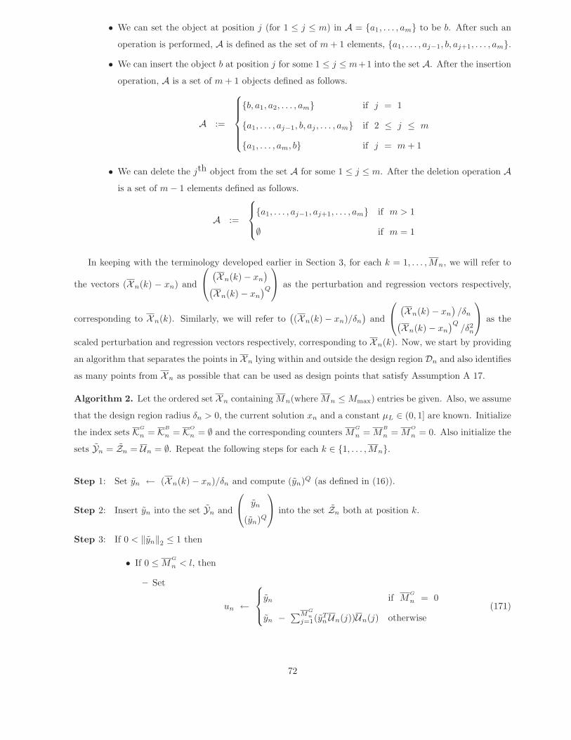
• We can set the object at position j (for 1 ≤ j ≤ m) in A = {a1, . . . , am} to be b. After such an

operation is performed, A is defined as the set of m + 1 elements, {a1, . . . , aj−1, b, aj+1, . . . , am}.

• We can insert the object b at position j for some 1 ≤ j ≤ m+1 into the set A. After the insertion

operation, A is a set of m + 1 objects defined as follows.

A :=

⎧⎪⎪⎪⎪⎨⎪⎪⎪⎪⎩{b, a1, a2, . . . , am} if j = 1

{a1, . . . , aj−1, b, aj , . . . , am} if 2 ≤ j ≤ m

{a1, . . . , am, b} if j = m + 1

• We can delete the jth object from the set A for some 1 ≤ j ≤ m. After the deletion operation Ais a set of m− 1 elements defined as follows.

A :=

⎧⎪⎨⎪⎩{a1, . . . , aj−1, aj+1, . . . , am} if m > 1

∅ if m = 1

In keeping with the terminology developed earlier in Section 3, for each k = 1, . . . ,Mn, we will refer to

the vectors (Xn(k) − xn) and

⎛⎝ (Xn(k)− xn

)(Xn(k)− xn

)Q

⎞⎠ as the perturbation and regression vectors respectively,

corresponding to Xn(k). Similarly, we will refer to((Xn(k)− xn)/δn

)and

⎛⎝ (Xn(k)− xn

)/δn(

Xn(k)− xn

)Q/δ2

n

⎞⎠ as the

scaled perturbation and regression vectors respectively, corresponding to Xn(k). Now, we start by providing

an algorithm that separates the points in Xn lying within and outside the design region Dn and also identifies

as many points from Xn as possible that can be used as design points that satisfy Assumption A 17.

Algorithm 2. Let the ordered set Xn containing Mn(where Mn ≤Mmax) entries be given. Also, we assume

that the design region radius δn > 0, the current solution xn and a constant μL ∈ (0, 1] are known. Initialize

the index sets KG

n = KB

n = KO

n = ∅ and the corresponding counters MG

n = MB

n = MO

n = 0. Also initialize the

sets Yn = Zn = Un = ∅. Repeat the following steps for each k ∈ {1, . . . ,Mn}.

Step 1: Set yn ← (Xn(k)− xn)/δn and compute (yn)Q (as defined in (16)).

Step 2: Insert yn into the set Yn and

⎛⎝ yn

(yn)Q

⎞⎠ into the set Zn both at position k.

Step 3: If 0 < ‖yn‖2 ≤ 1 then

• If 0 ≤MG

n < l, then

– Set

un ←

⎧⎪⎨⎪⎩

yn if MG

n = 0

yn −∑M

Gn

j=1(yTnUn(j))Un(j) otherwise

(171)

72

– If ‖yn‖2 < μL or ‖un‖2 < μL ‖yn‖2, then set MB

n ←MB

n +1 and insert k into the set KB

n

at the position MB

n .

– If ‖yn‖2 ≥ μL and ‖un‖2 ≥ μL ‖yn‖2 then

∗ Set MG

n ←MG

n + 1 and insert k into the set KG

n at the position MG

n .

∗ Insert (un/ ‖un‖2) into the set Un at the position MG

n .

• If MG

n = l, then set MB

n ←MB

n + 1 and insert k into the set KB

n at the position MB

n .

Step 4: If ‖yn‖2 > 1, then MO

n ←MO

n + 1 and insert k into the set KO

n at the position MO

n .

It is easily seen from the operation of Algorithm 2 that the various sets generated in the algorithm satisfy

the following properties.

P 3.14. For each k = 1, . . . ,Mn, Yn(k) and Zn(k) are respectively, the scaled perturbation and regression

vectors for the point Xn(k), evaluated with respect to xn.

P 3.15. 1. The setsKG

n , KB

n andKO

n , containing MG

n , MB

n and MO

n elements respectively, satisfyKG

n

⋂KB

n =

KB

n

⋂KO

n = KO

n

⋂KG

n = φ and KG

n

⋃KB

n

⋃KO

n ={1, . . . ,Mn

}. Consequently, we have M

G

n + MB

n +

MO

n = Mn.

2.∥∥∥Yn(KG

n(i))∥∥∥

2≤ 1 for each i = 1, . . . ,M

G

n and∥∥∥Yn(KB

n(i))∥∥∥

2≤ 1 for each i = 1, . . . ,M

B

n . Consequently,

we get that Xn(KG

n)⋃Xn(KB

n) ⊂ Dn, where Dn is the design region for iteration n defined as in (26).

Thus, the points in Xn(KG

n) and Xn(KB

n) together form a set of potential inner design points for

iteration n. Similarly∥∥∥Yn(KO

n(i))∥∥∥

2≥ 1 for each i = 1, . . . ,M

O

n and hence the points in Xn(KO

n) ∈R

l \ Dn form a set of potential outer design points for iteration n.

P 3.16. 1. If MG

n ≥ 1, the vectors in the set Un are the Gram-Schmidt vectors corresponding to those

in Yn(KG

n). That is, if MG

n ≥ 1, then

Un(1) =Yn(KG

n(1))∥∥∥Yn(KG

n(1))∥∥∥

2

(172)

and if MG

n ≥ 2 then for i = 2, . . . ,MG

n ,

Un(i) =Yn(KG

n(i))−∑i−1

j=1

(Yn(KG

n(i))TUn(j))Un(j)∥∥∥Yn(KG

n(i))−∑i−1

j=1

(Yn(KG

n(i))TUn(j))Un(j)

∥∥∥2

(173)

2. If MG

n ≥ 1, then for each i = 1, . . . ,MG

n ,

∥∥∥Yn(KG

n(i))∥∥∥

2≥ μL (174)

73

Further, if∣∣∣MG

n

∣∣∣ ≥ 2 then we get from Property P 3.13 that for i = 2, . . . ,∣∣∣MG

n

∣∣∣,∥∥∥∥Π

(Yn(KG

n(i)),(span

{Yn(KG

n(1)), . . . , Yn(KG

n(i− 1))})⊥)∥∥∥∥

2∥∥∥Yn(KG

n(i))∥∥∥

2

=

∥∥∥Yn(KG

n(i))−∑i−1

j=1

(Yn(KG

n(i))TUn(j))Un(j)

∥∥∥2∥∥∥Yn(KG

n(i))∥∥∥

2

≥ μL (175)

Indeed, it is easily seen that Algorithm 2 is only a slightly modified form of the Gram-Schmidt orthogonal-

ization process; the only difference being that in Algorithm 2, the set of vectors on which the Gram-Schmidt

process is performed i.e., Yn(KG

n), is chosen from Yn as the algorithm progresses, so as to ensure that the

vectors in Yn(KG

n) satisfy (174) and (175). Consequently, from Property P 3.16, it is clear that if MG

n ≥ 1

and we set xn + yin = Xn(KG

n(i)) for each i = 1, . . . ,MG

n , then (156) is satisfied for i = 1, . . . ,MG

n and if

MG

n ≥ 2, then (157) is satisfied for i = 2, . . . ,MG

n .

However, recall that l inner design points satisfying (156) and (157) are required to satisfy Assumption

A 17 and it is clearly possible that after Algorithm 2 is executed we get fewer than l points in Xn(KG

n), i.e.,

MG

n < l. Thus, we describe a procedure next, that inserts an appropriate point into Xn, such that MG

n is

incremented by one and the Properties P 3.14 through P 3.16 continue to hold.

Algorithm 3. Let us assume that we have knowledge of the design region radius δn, the sets Xn, Yn,

Zn, Nn, Fn, Φn and Un, the index sets KG

n , KB

n and KO

n and a constant μL ∈ (0, 1], such that Properties

P 3.14 through P 3.16 are satisfied. Further, we assume that MG

n < l and let {e1, . . . , el} ⊂ Rl represent the

standard orthonormal basis for Rl.

Step 1 : If MG

n = 0, then set yn ← e1.

Step 2 : If MG

n ≥ 1, then

• Find i∗ ∈ [1, . . . , l] such that

un = ei∗ −M

Gn∑

j=1

(ei∗TUn(j))Un(j) and ‖un‖2 > 0 (176)

• Set yn ← (un/ ‖un‖2).

Step 3 : Set Mn ←Mn + 1.

Step 4 : Insert yn into Yn,

⎛⎝ yn

(yn)Q

⎞⎠ into Zn and xn + δnyn into Xn all at position Mn.

Step 5 : Insert the value 0 into Fn, Φn and N n all at position Mn.

74

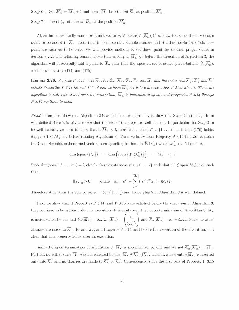
Step 6 : Set MG

n ←MG

n + 1 and insert Mn into the set KG

n at position MG

n .

Step 7 : Insert yn into the set Un at the position MG

n .

Algorithm 3 essentially computes a unit vector yn ∈ (span{Yn(KG

n)})⊥ sets xn + δnyn as the new design

point to be added to Xn. Note that the sample size, sample average and standard deviation of the new

point are each set to be zero. We will provide methods to set these quantities to their proper values in

Section 3.2.2. The following lemma shows that as long as MG

n < l before the execution of Algorithm 3, the

algorithm will successfully add a point to Xn such that the updated set of scaled perturbations Yn(KG

n),

continues to satisfy (174) and (175)

Lemma 3.20. Suppose that the sets Xn,Yn, Zn, Nn, Fn, Φn and Un and the index sets KG

n, KB

n and KO

n

satisfy Properties P 3.14 through P 3.16 and we have MG

n < l before the execution of Algorithm 3. Then, the

algorithm is well defined and upon its termination, MG

n is incremented by one and Properties P 3.14 through

P 3.16 continue to hold.

Proof. In order to show that Algorithm 2 is well defined, we need only to show that Steps 2 in the algorithm

well defined since it is trivial to see that the rest of the steps are well defined. In particular, for Step 2 to

be well defined, we need to show that if MG

n < l, there exists some i∗ ∈ {1, . . . , l} such that (176) holds.

Suppose 1 ≤ MG

n < l before running Algorithm 3. Then we know from Property P 3.16 that Un contains

the Gram-Schmidt orthonormal vectors corresponding to those in Yn(KG

n) where MG

n < l. Therefore,

dim(span

{Un

})= dim

(span

{Yn(KG

n)})

= MG

n < l

Since dim(span{e1, . . . , el}) = l, clearly there exists some i∗ ∈ {1, . . . , l} such that ei∗ /∈ span{Un}, i.e., such

that

‖un‖2 > 0, where un = ei∗ −|Un|∑j=1

((ei∗)TUn(j))Un(j)

Therefore Algorithm 3 is able to set yn = (un/ ‖un‖2) and hence Step 2 of Algorithm 3 is well defined.

Next we show that if Properties P 3.14, and P 3.15 were satisfied before the execution of Algorithm 3,

they continue to be satisfied after its execution. It is easily seen that upon termination of Algorithm 3, Mn

is incremented by one and Yn(Mn) = yn, Zn(Mn) =

⎛⎝ yn

(yn)Q

⎞⎠ and Xn(Mn) = xn + δnyn. Since no other

changes are made to Xn, Yn and Zn, and Property P 3.14 held before the execution of the algorithm, it is

clear that this property holds after its execution.

Similarly, upon termination of Algorithm 3, MG

n is incremented by one and we get KG

n(MG

n) = Mn.

Further, note that since Mn was incremented by one, Mn /∈ KB

n

⋃KO

n . That is, a new entry(Mn) is inserted

only into KG

n and no changes are made to KB

n or KO

n . Consequently, since the first part of Property P 3.15

75

was assumed to hold before the execution of Algorithm 3, it continues to hold after the execution of the

algorithm. Further, since∥∥∥Yn(Mn)

∥∥∥2

= ‖yn‖2 = 1 (where yn is calculated in either Step 1 or Step 2), it is

clear that Xn(Mn) ∈ Dn. Therefore, after the execution of the algorithm Xn(KG

n) ⊂ Dn, Xn(KB

n) ⊂ Dn and

Xn(KO

n) ⊂ Rl \ Dn and the second part of Property P 3.15 continues to hold.

Next, let us show that if Property P 3.16 held before the execution of Algorithm 3, then it holds after

its execution. Note again, that upon termination of the algorithm, the value of MG

n is incremented by one

and Un(MG

n) = Yn(KG

n(MG

n)) = yn. First, if MG

n = 0 before the execution of Algorithm 3, then after its

execution MG

n = 1 and Un(MG

n) = Yn(KG

n(MG

n)) = e1. Thus, it is clear that (172) holds. Further, since∥∥∥Yn(MG

n)∥∥∥

2= 1, it is easily seen that (174) is satisfied for i = 1.

Finally, suppose that MG

n ≥ 1 before the execution of Algorithm 3. Then, MG


and consequently, MG

n ≥ 2 after its execution. Since we assumed that the first part of Property P 3.16 held

before the algorithm was executed, we know that after it is executed, (172) holds and if MG

n ≥ 3 after the

execution of the algorithm then (173) holds for i = 2, . . . MG

n − 1. Therefore, from Property P 3.11, we get

that {Un(1), . . . ,Un(MG

n − 1)} is an orthonormal set. Using this in (176), we get that

uTnUn(j) = (ei∗)TUn(j)− (ei∗)TUn(j) = 0 for each j = 1, . . . ,M

G

n − 1

Thus, since yn = (un/ ‖un‖2), we get that ‖yn‖2 = 1 and

(yn)T Un(j) = 0 for each j = 1, . . . ,MG

n − 1 (177)

Since Un(MG

n) = Yn(KG

n(MG

n)) = yn, we get using (177) and ‖yn‖2 = 1, that

Un(MG

n) = yn =yn −

∑MGn −1

j=1

(yT

nUn(j))Un(j)∥∥∥∥yn −

∑MGn −1

j=1

(yT

nUn(j))Un(j)

∥∥∥∥2

=Yn(KG

n(MG

n))−∑M

Gn −1

j=1

(Yn(KG

n(MG

n))TUn(j))Un(j)∥∥∥∥Yn(KG

n(MG

n))−∑M

Gn −1

j=1

(Yn(KG

n(MG

n))TUn(j))Un(j)

∥∥∥∥2

Therefore, (173) holds for i = MG

n . Thus, the first part of Property P 3.16 holds after the execution of

Algorithm 3.

Similarly, since the second part of Property P 3.16 was assumed to hold before the execution of Al-

gorithm 3, we get that after its execution (174) holds for i = 1, . . . ,MG

n − 1 and if MG

n ≥ 3, (175) holds

for i = 2, . . . ,MG

n − 1. Thus, in order to show that the second part of Property P 3.16 holds after the

execution of Algorithm 3, we only have to show that (174) and (175) hold for i = MG

n . Obviously, since∥∥∥Yn(KG

n(MG

n))∥∥∥

2= ‖yn‖2 = 1 ≥ μL, (174) holds for i = M

G

n . Further, we get using Property P 3.13 and

76

(177), that

∥∥∥∥Π(Yn(KG

n(MG

n)),(span

{Yn(KG

n(1)), . . . , Yn(KG

n(MG

n − 1))})⊥)∥∥∥∥

2∥∥∥Yn(KG

n(MG

n))∥∥∥

2

=

∥∥∥∥yn −∑M

Gn −1

j=1

((yn)T Un(j)

)Un(j)

∥∥∥∥2

‖yn‖2=‖yn‖2‖yn‖2

= 1 ≥ μL

Therefore (175) holds for i = MG

n and consequently, the second part of Property P 3.16 continues to hold

upon termination of Algorithm 3.

Now if we have the set Xn (and the corresponding N n, Fn and Φn) for each n ∈ N, we can use

Algorithms 2 and 3 to find a set of design points {xn + yin : i = 1, . . . , Mn} such that Assumptions A 16 and

A 17 are satisfied.

Algorithm 4. Let us assume that for each n ∈ N, we have the sets Xn, N n, Fn and Φn with Mn ≤Mmax.

Initialize the index sets KGn = KB

n = KOn = ∅ and the corresponding counters MG

n = MBn = MO

n = 0. Let the

constant l ≥M Imax <∞ be given.

Step 1 : Run Algorithm 2 once. Then, run Algorithm 3 as many times as necessary to obtain the sets

Yn, Zn, Un and the index sets KG

n , KB

n and KO

n with MG

n = l, MB

n and MO

n elements respectively.

Note that Algorithm 3 has to be run at most l times since the value of MG


whenever Algorithm 3 is run.

Step 2 : Set KGn ← K

G

n and MGn ←M

G

n .

Step 3 : Set the index set KBn with 0 ≤ MB

n ≤ min{

MB

n ,M Imax − l

}elements, such that it contains a

subset of the elements in KB

n in some order (the order can be chosen arbitrarily). For example,

we may set KBn ← ∅ or KB

n ← KB

n or KBn ←

{i ∈ KB

n : N n(KB

n(i)) ≥ αN0n

}for some constant

α ∈ (0, 1].

Step 4 : Set the index set KOn with 0 ≤MO

n ≤MO

n elements, such that it contains a subset of the elements

in KO

n in some order (the order can be chosen arbitrarily). For example, we may set KOn ← 0 or

KOn ← K

O

n or KOn ←

{i ∈ KO

n :∥∥∥Yn(KO

n(i))∥∥∥

2≤ αδ

}for some constant αδ > 1.

Step 5 : For each i = 1, . . . ,MGn , set xn + yi

n ← Xn (KGn (i)).

Step 6 : If MBn > 0, then

• For each i = MGn + 1, . . . , MG

n + MBn , set xn + yi

n ← Xn (KBn (i−MG

n )).

Step 7 : If MOn > 0, then

77

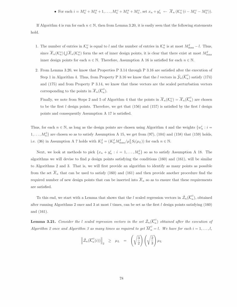
• For each i = MGn + MB

n + 1, . . . ,MGn + MB

n + MOn , set xn + yi

n ← Xn (KOn (i−MG

n −MBn )).

If Algorithm 4 is run for each n ∈ N, then from Lemma 3.20, it is easily seen that the following statements

hold.

1. The number of entries in KGn is equal to l and the number of entries in KB

n is at most M Imax − l. Thus,

since Xn(KGn)⋃Xn(KB

n) form the set of inner design points, it is clear that there exist at most M Imax

inner design points for each n ∈ N. Therefore, Assumption A 16 is satisfied for each n ∈ N.

2. From Lemma 3.20, we know that Properties P 3.14 through P 3.16 are satisfied after the execution of

Step 1 in Algorithm 4. Thus, from Property P 3.16 we know that the l vectors in Yn(KG

n) satisfy (174)

and (175) and from Property P 3.14, we know that these vectors are the scaled perturbation vectors

corresponding to the points in Xn(KG

n).

Finally, we note from Steps 2 and 5 of Algorithm 4 that the points in Xn(KGn) = Xn(KG

n) are chosen

to be the first l design points. Therefore, we get that (156) and (157) is satisfied by the first l design

points and consequently Assumption A 17 is satisfied.

Thus, for each n ∈ N, as long as the design points are chosen using Algorithm 4 and the weights {win : i =

1, . . . ,M In} are chosen so as to satisfy Assumption A 15, we get from (97), (104) and (158) that (159) holds,

i.e. (36) in Assumption A 7 holds with KIλ = (KI

wM Imax/μ2

LSl(μL)) for each n ∈ N.

Next, we look at methods to pick {xn + yin : i = 1, . . . ,M I

n} so as to satisfy Assumption A 18. The

algorithms we will devise to find p design points satisfying the conditions (160) and (161), will be similar

to Algorithms 2 and 3. That is, we will first provide an algorithm to identify as many points as possible

from the set Xn that can be used to satisfy (160) and (161) and then provide another procedure find the

required number of new design points that can be inserted into Xn so as to ensure that these requirements

are satisfied.

To this end, we start with a Lemma that shows that the l scaled regression vectors in Zn(KG

n), obtained

after running Algorithms 2 once and 3 at most l times, can be set as the first l design points satisfying (160)

and (161).

Lemma 3.21. Consider the l scaled regression vectors in the set Zn(KG

n) obtained after the execution of

Algorithm 2 once and Algorithm 3 as many times as required to get MG

n = l. We have for each i = 1, . . . , l,

∥∥∥Zn(KG

n(i))∥∥∥

2≥ μL =

(√32

)(√23

)μL

78

and for i = 2, . . . , l,∥∥∥∥Π(Zn(KG

n(i)),(span{Zn(KG

n(1)), . . . , Zn(KG

n(i− 1))})⊥)∥∥∥∥

2∥∥∥Zn(KG

n(i))∥∥∥

2

≥(√

23

)μL

Consequently, the Gram-Schmidt orthogonalization process can be successfully performed on the l vectors in

Zn(KG

n).

Proof. First we note that from Lemma 3.20, the l vectors in Yn(KG

n) obtained after running Algorithm 2

once and Algorithm 3 at most l times, satisfy Properties P 3.14 through P 3.16. Now, from (17) it is easy

to see that for each i = 1, . . . , l.∥∥∥Zn(KG

n(i))∥∥∥

2=

√∥∥∥Yn(KG

n(i))∥∥∥2

2+

12

∥∥∥Yn(KG

n(i))∥∥∥4

2

From Property P 3.15, we know that∥∥∥Yn(KG

n(i))∥∥∥

2≤ 1. Using this, we get

∥∥∥Yn(KG

n(i))∥∥∥

2≤

∥∥∥Zn(KG

n(i))∥∥∥

2≤

√32

∥∥∥Yn(KG

n(i))∥∥∥

2(178)

Since (174) in Property P 3.16 holds, we get from (178) that for each i = 1, . . . , l,

∥∥∥Zn(KG

n(i))∥∥∥

2≥

∥∥∥Yn(KG

n(i))∥∥∥

2≥ μL =

(√32

)(√23

)μL > 0

Next, for each i = 2, . . . , l, we get using the definition of the orthogonal projection operator, that∥∥∥∥Π(Zn(KG

n(i)),(span

{Zn(KG

n(j)) : j = 1, . . . , i− 1})⊥)∥∥∥∥

2

=∥∥∥Zn(KG

n(i))−Π(Zn(KG

n(i)), span{Zn(KG

n(j)) : j = 1, . . . , i− 1})∥∥∥

2=

min{∥∥∥Zn(KG

n(i))− v∥∥∥

2: v ∈ span

{Zn(KG

n(j)) : j = 1, . . . , i− 1}}

Clearly any v ∈ span{Zn(KG

n(j))) : j = 1, . . . , i− 1}

can be written as v =∑i−1

j=1 αjZn(KG

n(j)) for some

α1, . . . , αi−1 ∈ R. Therefore,

min{∥∥∥Zn(KG

n(i))− v∥∥∥

2: v ∈ span

{Zn(KG

n(j)) : j = 1, . . . , i− 1}}

=

minα1,...,αi−1∈R

∥∥∥∥∥∥Zn(KG

n(i))−i−1∑j=1

αjZn(KG

n(j))

∥∥∥∥∥∥2

Further, using the definition of Zn(KG

n(i)) for i = 1, . . . , l, we get that for any α1, . . . , αi−1 ∈ R,∥∥∥∥∥∥Zn(KG

n(i))−i−1∑j=1

αjZn(KG

n(j))

∥∥∥∥∥∥2

=

∥∥∥∥∥∥⎛⎝ Yn(KG

n(i))(Yn(KG

n(i)))Q

⎞⎠− i−1∑

j=1

⎧⎨⎩αj

⎛⎝ Yn(KG

n(j))(Yn(KG

n(i)))Q

⎞⎠⎫⎬⎭∥∥∥∥∥∥

2

≥

∥∥∥∥∥∥Yn(KG

n(i))−i−1∑j=1

αjYn(KG

n(j))

∥∥∥∥∥∥2

79

Thus, we have for each i = 2, . . . , l,∥∥∥∥Π(Zn(KG

n(i)),(span

{Zn(KG

n(j)) : j = 1, . . . , i− 1})⊥)∥∥∥∥

2

= minα1,...,αi−1∈R

∥∥∥∥∥∥Zn(KG

n(i))−i−1∑j=1

αjZn(KG

n(j))

∥∥∥∥∥∥2

≥ minα1,...,αi−1∈R

∥∥∥∥∥∥Yn(KG

n(i))−i−1∑j=1

αjYn(KG

n(j))

∥∥∥∥∥∥2

=∥∥∥Yn(KG

n(i))−Π(Yn(KG

n(i)), span{Yn(KG

n(j)) : j = 1, . . . , i− 1})∥∥∥

2

=∥∥∥∥Π

(Yn(KG

n(i)),(span

{Yn(KG

n(j)) : j = 1, . . . , i− 1})⊥)∥∥∥∥

2

Finally, using (178) and (175) in Property P 3.16, we get for each i = 2, . . . , l,∥∥∥∥Π(Zn(KG

n(i)),(span

{Zn(KG

n(j)) : j = 1, . . . , i− 1})⊥)∥∥∥∥

2∥∥∥Zn(KG

n(i))∥∥∥

2

≥

(√23

)⎛⎜⎜⎝∥∥∥∥Π

(Yn(KG

n(i)),(span

{Yn(KG

n(j)) : j = 1, . . . , i− 1})⊥)∥∥∥∥

2∥∥∥Yn(KG

n(i))∥∥∥

2

⎞⎟⎟⎠ ≥

(√23

)μL

Consequently, using Lemma 3.12, we get that {Zn(KG

n(1)), . . . , Zn(KG

n(l))} ⊂ Rp is a linearly independent

set and therefore, we can perform Gram-Schmidt orthogonalization on this set.

Thus, if we set the first l design points {xn + yin : i = 1, . . . , l} to be those in Xn(KG

n), then from

Lemma 3.21, it is clear that (160) and (161) in Assumption A 18 are satisfied for i = 1, . . . , l with μQ =(√2/3

)μL. The advantages of such a “warm start” are obvious. First, by running Algorithm 2 we have

already separated the potential inner and outer design points in Xn. Also, in order satisfy Assumption A 18,

instead of having to pick p design points, we only have to find p − l additional points. Finally, if for any

reason, we wish to stop without picking the required p− l design points we are still assured of the bound on

the condition number of (Y In )T W I

n Y In as in (159).

Motivated by Lemma 3.21, we provide an algorithm next that performs the Gram-Schmidt orthogonal-

ization process on the scaled regression vectors corresponding to the points in Xn(KG

n) and searches the set

Xn(KB

n) for more points that can be used to satisfy Assumption A 18.

Algorithm 5. Let us assume that we have knowledge of the design region radius δn, the sets Xn, Yn, Zn,

Nn, Fn and Φn, the index sets KG

n , KB

n and KO

n such that Properties P 3.14 through P 3.16 are satisfied.

Further, we assume that MG

n = l. Initialize the set Vn = ∅. Choose a constant μQ1 ∈ (0, 1].

Step 1 : Repeat the following steps for each i = 1, . . . ,MG

n .

80

• If i = 1, then set vn ← Zn(KG

n(i)).

• If i ≥ 2, then set

vn ← Zn(KG

n(i))−i−1∑j=1

(Zn(KG

n(i))TVn(j))Vn(j)

• Insert (vn/ ‖vn‖2) into the set Vn at position i.

Step 2 : Repeat the following steps for i = 1, . . . ,MB

n .

• If MG

n < p then

– Set

vn ← Zn(KB

n(i))−M

Gn∑

j=1

(Zn(KB

n(i))TVn(j))Vn(j) (179)

– If∥∥∥Zn(KB

n(i))∥∥∥

2≥ (

√3/2)μQ1 and ‖vn‖2 ≥ μQ1

∥∥∥Zn(KB

n(i))∥∥∥

2then

∗ Set MG

n ←MG

n + 1.

∗ Insert KB

n(i) into the set KG

n at position MG

n .

∗ Insert (vn/ ‖vn‖2) into the set Vn at the position MG

n .

– Otherwise if∥∥∥Zn(KB

n(i))∥∥∥

2< (

√3/2)μQ1 or ‖vn‖2 < μQ1

∥∥∥Zn(KB

n(i))∥∥∥

2, then set M tmp ←

M tmp + 1 and insert KB

n(i) into the set Ktmpat position M tmp.

• Otherwise if MG

n = p then set M tmp ← M tmp + 1 and insert KB

n(i) into the set Ktmpat

position M tmp.

Step 3 : Set KB

n ← Ktmp

and MB

n ←M tmp.

We know from Lemma 3.21 that we can perform Gram-Schmidt orthogonalization on the vectors in

Zn(KG

n). Step 1 of Algorithm 5 does exactly this. Step 2 checks each scaled regression vector Zn(KB

n(i)) for

i = 1, . . . ,MB

n , to see if it satisfies

∥∥∥Zn(KB

n(i))∥∥∥

2≥

(√32

)μQ1 and

∥∥∥∥Π(Zn(KB

n(i)), span{Zn(KG

n)}⊥)∥∥∥∥

2∥∥∥Zn(KB

n(i))∥∥∥

2

≥ μQ1

If it does then the index KB

n(i) is moved to KG

n and the set Vn containing the Gram-Schmidt vectors

corresponding to those in Zn(KG

n) is updated appropriately. Thus, it is easily seen that after the execution

of Algorithm 5, Properties P 3.14 and P 3.15 continue to hold. Further from Lemma 3.21 and Steps 1 and

2 of Algorithm 5 it can be seen that, the sets Zn(KG

n) and Vn satisfy the following property (analogous to

Property P 3.16) for μQ = min{μQ1, (√

2/3)μL}.

P 3.17. 1. The vectors in the set Vn are the Gram-Schmidt orthonormal vectors corresponding to those

in Zn(KG

n). That is,

Vn(1) =Zn(KG

n(1))∥∥∥Zn(KG

n(1))∥∥∥

2

(180)

81

and for i = 2, . . . ,MG

n ,

Vn(i) =Zn(KG

n(i))−∑i−1

j=1

(Zn(KG

n(i))TVn(j))Vn(j)∥∥∥Zn(KG

n(i))−∑i−1

j=1

(Zn(KG

n(i))TVn(j))Vn(j)

∥∥∥2

(181)

2. The MG

n vectors in Zn(KG

n) satisfy for each i = 1, . . . ,MG

n ,∥∥∥Zn(KG

n(i))∥∥∥

2≥

(√32

)μQ (182)

and from Property P 3.13, we get that for i = 2, . . . ,MG

n ,∥∥∥∥Π(Zn(KG

n(i)),(span

{Zn(KG

n({1, . . . , i− 1}))})⊥)∥∥∥∥

2∥∥∥Zn(KG

n(i))∥∥∥

2

=

∥∥∥Zn(KG

n(i))−∑i−1

j=1

(Zn(KG

n(i))TVn(j))Vn(j)

∥∥∥2∥∥∥Zn(KG

n(i))∥∥∥

2

≥ μQ (183)

From Property P 3.17, it is clear that upon termination of Algorithm 5, we can set the first MG

n design

points to be those in Xn(KG

n) and satisfy (160) and (161) in Assumption A 18 with μQ = min{μQ1, (√

2/3)μL}.However, in order to satisfy Assumption A 18, we require p inner design points satisfying (160) and (160),

and it is clearly possible that after the execution of Algorithm 5, we get MG

n < p. Accordingly we provide

next, an algorithm analogous to Algorithm 3, that adds an appropriate point into Xn and increments MG

n

by one such that Properties P 3.14 through Property P 3.17 continue to hold.

Let us recall the operation of Algorithm 3. There, if dim(span{Yn(KG

n)}) = MG

n < l, we merely found a

unit vector yn ∈ span{(Yn(KG

n))⊥} and inserted xn + δnyn to Xn. Now, if dim(span{Zn(KG

n)}) = MG

n < p,

we could, in the same manner, find a unit vector wn ∈ span{(Zn(KG

n))⊥}. However, in this case, in order to

be able to insert a point to Xn, wn has to have a very specific form. That is, we can add a point xn + δnyn

to Xn only if wn ∈ span{(Zn(KG

n))⊥} is such that

wn =

⎛⎝ yn

(yn)Q

⎞⎠

The following two lemmas show that even though we cannot pick any arbitrary wn ∈ span{(Zn(KG

n))⊥},

there exists an appropriate vector zn =

⎛⎝ yn

(yn)Q

⎞⎠ sufficiently close to wn, such that xn+δnyn can be inserted

into Xn.

Lemma 3.22. Consider any w1 ∈ Rp with ‖w1‖2 = 1. Then, there exists z ∈ R

p given by z =

⎛⎝ y

yQ

⎞⎠ for

some y ∈ Rl, such that ‖y‖2 ≤ 1 and∣∣zT w1

∣∣ =∣∣∣(yT

(yQ)T)

w1

∣∣∣ ≥ 12√

p(184)

82

Further, given any such z ∈ Rp and a subspace M⊂ R

p such that w1 ∈M⊥, we have

‖z‖2 ≥(√

32

)(1√6p

)and

∥∥Π (z,M⊥)∥∥

2

‖z‖2≥ 1√

6p

Proof. Define the vector w ∈ Rp as

w :=w1

‖w1‖∞Then clearly, we have ‖w‖∞ = 1. Now, let the components of w ∈ R

p be as follows,

wT =(u1 , . . . , ul , v12 , v13 , v23 , . . . , v1l , . . . , v(l−1)l , v11 , . . . , vll

)Then, since ‖w‖∞ = 1, we get that one of the following cases must hold

(a) |uj∗ | = 1 for some j∗ ∈ {1, . . . , l}.

(b) |vj∗j∗ | = 1 for some j∗ ∈ {1, . . . , l}.

(c) |vj∗k∗ | = 1 for some j∗, k∗ ∈ {1, . . . , l} where j∗ �= k∗.

Let for any y ∈ Rl, the components of y be given as yT =

(y1 . . . yl

). Then, from (16), we get that

(yT

(yQ)T)

=(y1 , . . . , yl , y1y2 , y1y3 , y2y3 , . . . , y1yl , . . . , yl−1yl , 1√

2y21 , . . . , 1√

2y2

l

)Thus, for any y ∈ R

l, we get that

∣∣∣(yT(yQ)T)

w∣∣∣ =

⎧⎨⎩

l∑j=1

(uj yj +

1√2vjj y

2j

)⎫⎬⎭ +

⎧⎨⎩

l∑k=2

k−1∑j=1

vjkyj yk

⎫⎬⎭

Also, we will use the following identity repeatedly in our proof.

max {|αj | : j = 1, . . . , N} ≥

√∑Nj=1 |αj |2

Nfor any α1, . . . , αN ∈ R (185)

Now, let use consider the three cases, listed earlier in order.

(a) Suppose that |uj∗ | = 1 for some j∗ ∈ {1, . . . , l}. Then consider the following two points y1, y2 ∈ Rl.

(y1)T =(y11 . . . y1

l

)where y1

j∗ = 1 and y1j = 0 for j �= j∗

(y2)T =(y21 . . . y2

l

)where y2

j∗ = −1 and y2j = 0 for j �= j∗

(186)

83

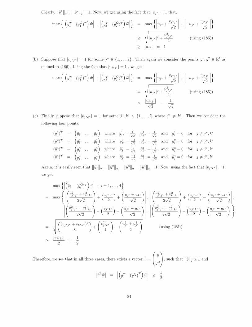
Clearly,∥∥y1

∥∥2

=∥∥y2

∥∥2

= 1. Now, we get using the fact that |uj∗ | = 1 that,

max{∣∣∣(yT

1 (yQ1 )T

)w∣∣∣ ,

∣∣∣(yT2 (yQ

2 )T)

w∣∣∣} = max

{∣∣∣∣uj∗ +vj∗j∗√

2

∣∣∣∣ ,

∣∣∣∣−uj∗ +vj∗j∗√

2

∣∣∣∣}

≥

√|uj∗ |2 +

v2j∗j∗

2(using (185))

≥ |uj∗ | = 1

(b) Suppose that |vj∗j∗ | = 1 for some j∗ ∈ {1, . . . , l}. Then again we consider the points y1, y2 ∈ Rl as

defined in (186). Using the fact that |vj∗j∗ | = 1 , we get

max{∣∣∣(yT

1 (yQ1 )T

)w∣∣∣ ,

∣∣∣(yT2 (yQ

2 )T)

w∣∣∣} = max

{∣∣∣∣uj∗ +vj∗j∗√

2

∣∣∣∣ ,

∣∣∣∣−uj∗ +vj∗j∗√

2

∣∣∣∣}

=

√|uj∗ |2 +

v2j∗j∗

2(using (185))

≥ |vj∗j∗ |√2

=1√2

(c) Finally suppose that |vj∗k∗ | = 1 for some j∗, k∗ ∈ {1, . . . , l} where j∗ �= k∗. Then we consider the

following four points.

(y1)T =(y11 . . . y1

l

)where y1

j∗ = 1√2, y1

k∗ = 1√2

and y1j = 0 for j �= j∗, k∗

(y2)T =(y21 . . . y2

l

)where y2

j∗ = −1√2

y1k∗ = −1√

2and y2

j = 0 for j �= j∗, k∗

(y3)T =(y31 . . . y3

l

)where y3

j∗ = 1√2

y1k∗ = −1√

2and y3

j = 0 for j �= j∗, k∗

(y4)T =(y41 . . . y4

l

)where y4

j∗ = −1√2

y1k∗ = 1√

2and y4

j = 0 for j �= j∗, k∗

Again, it is easily seen that∥∥y1

∥∥2

=∥∥y2

∥∥2

=∥∥y3

∥∥2

=∥∥y4

∥∥2

= 1. Now, using the fact that |vj∗k∗ | = 1,

we get

max{∣∣∣(yT

i (yQi )T

)w∣∣∣ : i = 1, . . . , 4

}= max

{∣∣∣∣∣(

v2j∗j∗ + v2

k∗k∗

2√

2

)+(vj∗k∗

2

)+(

uj∗ + uk∗√2

)∣∣∣∣∣ ,∣∣∣∣∣(

v2j∗j∗ + v2

k∗k∗

2√

2

)+(vj∗k∗

2

)−(

uj∗ + uk∗√2

)∣∣∣∣∣ ,∣∣∣∣∣(

v2j∗j∗ + v2

k∗k∗

2√

2

)−(vj∗k∗

2

)+(

uj∗ − uk∗√2

)∣∣∣∣∣ ,∣∣∣∣∣(

v2j∗j∗ + v2

k∗k∗

2√

2

)−(vj∗k∗

2

)−(

uj∗ − uk∗√2

)∣∣∣∣∣}

=

√√√√((vj∗j∗ + vk∗k∗)2

8

)+

(v2

j∗k∗

4

)+

(u2

j∗ + u2j∗

2

)(using (185))

≥ |vj∗k∗ |2

=12

Therefore, we see that in all three cases, there exists a vector z =

⎛⎝ y

yQ

⎞⎠, such that ‖y‖2 ≤ 1 and

∣∣zT w∣∣ =

∣∣∣(yT(yQ)T)

w∣∣∣ ≥ 1

2

84

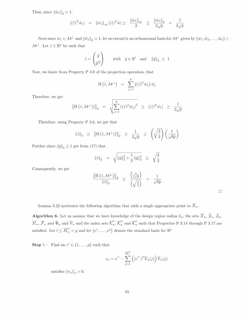
Thus, since ‖w1‖2 = 1,

|(z)T w1| = ‖w1‖∞ |(z)T w| ≥ ‖w1‖∞2

≥ ‖w1‖22√

p=

12√

p

Next since w1 ∈M⊥ and ‖w1‖2 = 1, let us extend it an orthonormal basis forM⊥ given by {w1, w2, . . . , wk} ⊂M⊥. Let z ∈ R

p by such that

z =

⎛⎝ y

yQ

⎞⎠ with y ∈ R

l and ‖y‖2 ≤ 1

Now, we know from Property P 3.8 of the projection operation, that

Π(z,M⊥) =

k∑j=1

((z)T wj

)wj

Therefore, we get ∥∥Π (z,M⊥)

)∥∥2

=

√√√√ k∑j=1

((z)T wj)2 ≥ |(z)T w1| ≥

12√

p

Therefore, using Property P 3.6, we get that

‖z‖2 ≥∥∥Π (

z,M⊥))∥∥

2≥ 1

2√

p≥

(√32

)(1√6p

)

Further since ‖y‖2 ≤ 1 get from (17) that

‖z‖2 =

√‖y‖22 +

12‖y‖42 ≤

√32

Consequently, we get ∥∥Π (z,M⊥)∥∥

2

‖z‖2≥

(1

2√

p

)(√

32

) =1√6p

Lemma 3.22 motivates the following algorithm that adds a single appropriate point to Xn.

Algorithm 6. Let us assume that we have knowledge of the design region radius δn, the sets Xn, Yn, Zn,

Nn, Fn and Φn and Vn and the index sets KG

n , KB

n and KO

n such that Properties P 3.14 through P 3.17 are

satisfied. Let l ≤MG

n < p and let {e1, . . . , ep} denote the standard basis for Rp

Step 1 : Find an i∗ ∈ {1, . . . , p} such that

vn = ei∗ −M

Gn∑

j=1

((ei∗)TVn(j)

)Vn(j)

satisfies ‖vn‖2 > 0.

85

Step 2 : Compute zn =

⎛⎝ yn

(yn)Q

⎞⎠ ∈ R

p with yn ∈ Rl such that ‖yn‖2 ≤ 1 and

∣∣∣∣zTn

(vn

‖vn‖2

)∣∣∣∣ ≥ 12√

p(187)

Step 3 : Set Mn ←Mn + 1.

Step 4 : Insert yn into Yn, zn into Zn and xn + δnyn into Xn all at position Mn.

Step 5 : Insert the value 0 into Fn, Φn and N n all at position Mn.

Step 6 : Set MG

n ←MG

n + 1 and insert Mn into the set KG

n at position MG

n .

Step 7 : Set

vn ← zn −M

Gn −1∑

j=1

(zTnVn(j)

)Vn(j)

Step 8 : Insert (vn/ ‖vn‖2) into Vn at position MG

n .

Note: In Step 2, we could potentially calculate the vector zn =

⎛⎝ yn

yQn

⎞⎠ as

zn ∈ arg max

⎧⎨⎩∣∣∣∣zT

(vn

‖vn‖2

)∣∣∣∣ : z =

⎛⎝ y

yQ

⎞⎠ where y ∈ R

l and ‖y‖2 ≤ 1

⎫⎬⎭ (188)

If zn is chosen as in (188), then clearly, from Lemma 3.22, (187) is satisfied. However, to find zn as in (188),

it is easily seen that we need to solve two nonlinearly constrained quadratic optimization problems which

could be computationally expensive. Alternatively, we can find an appropriate vector zn satisfying (187) by

a simple enumeration as shown in the proof of Lemma 3.22.

The following lemma shows that as long as MG

n < p before the execution of Algorithm 6, the algorithm

successfully inserts an appropriate point into Xn such that Properties P 3.14 and P 3.15 continue to hold

and Property P 3.17 continues to hold.

Lemma 3.23. Suppose that the sets Xn,Yn, Zn, Nn, Fn, Φn and Vn and the index sets KG

n, KB

n and

KO

n satisfy Properties P 3.14 and P 3.15 and Property P 3.17 for μQ = min{(√

2/3)μL, μQ1, (1/√

6p)} and

we have MG

n < p before the execution of Algorithm 6. Then, the algorithm is well defined and upon its

termination, an appropriate point is added to Xn and MG

n is incremented by one such that Properties P 3.14

and P 3.15 continue to hold and Property P 3.17 holds for μQ = min{(√

2/3)μL, μQ1, (1/√

6p)}.

Proof. First we show that as long as MG

n < p before the execution of Algorithm 6, all its steps are well

defined. Let us begin with Step 1. From our assumptions we know that MG

n < p before the execution of the

86

algorithm. Since Property P 3.17 holds before the execution of the algorithm, we know from the first part

of this property that Vn contains a set of MG

n < p Gram-Schmidt vectors corresponding to those in Zn(KG

n).

Therefore, dim(span{Vn}) = dim(span

{Zn(KG

n)})

= MG

n < p. Since dim(span{e1, . . . , ep}) = p, clearly

there exists i∗ ∈ {1, . . . , p} such that ei∗ /∈ span{Vn}, i.e., such that

‖vn‖2 =

∥∥∥∥∥∥ei∗ −M

Gn∑

j=1

((ei∗)TVn(j)

)Vn(j)

∥∥∥∥∥∥2

=∥∥∥∥Π

(ei∗ ,

(span{Zn(KG

n)})⊥)∥∥∥∥

2

> 0

Therefore, Step 1 is well defined. We know from Lemma 3.22, that there exists yn ∈ Rl with ‖yn‖2 ≤ 1 such

that (187) holds. Therefore, Step 2 in Algorithm 6 is well defined. It is trivial to see that the rest of the

steps in the algorithm are well defined and consequently that the algorithm itself is well defined.

Next we show that if Properties P 3.14, P 3.15 and P 3.17 were satisfied before the execution of Algo-

rithm 6, they continue to be satisfied after its execution. It is clear that upon termination of Algorithm 6,

Mn is incremented by one and Yn(Mn) = yn, Zn(Mn) =

⎛⎝ yn

(yn)Q

⎞⎠ and Xn(Mn) = xn + δnyn. Since no

other changes are made to Xn, Yn and Zn and Property P 3.14 we assumed to hold before the algorithms

execution, it is clear that this property continues to hold. Further, we also know that Algorithm 6 increments

MG

n by one and sets KG

n(MG

n) = Mn. It is easily seen that the incremented value of Mn cannot lie in either

KB

n or KO

n . Thus, since a new entry(Mn) is inserted only into KG

n and no changes are made to KB

n or KO

n ,

the first part of Property P 3.15 continues to hold after the execution of Algorithm 6. Finally, since yn as

defined in (187) in Step 2 satisfies ‖yn‖2 ≤ 1, it is also is clear that the second part of Property P 3.15

continues to hold.

Next, let us show that if Property P 3.17 holds before the execution of Algorithm 6 for μQ = min{(√

2/3)μL, μQ1, (1/√

6p)

then the property holds after the execution of Algorithm 6 for the same value of μQ. Note again that upon

termination of the algorithm, the value of MG

n is incremented by one with Zn(KG

n(MG

n)) = zn and from

Step 8,

Vn(MG

n) =Zn(KG

n(MG

n))−∑M

Gn −1

j=1

(Zn(KG

n(MG

n))TVn(j))Vn(j)∥∥∥∥Zn(KG

n(MG

n))−∑M

Gn −1

j=1

(Zn(KG

n(MG

n))TVn(j))Vn(j)

∥∥∥∥2

(189)

Since the first part Property P 3.17 held before the execution of the algorithm, clearly after its execution,

(180) holds and (181) holds for i = 2, . . . ,MG

n − 1. From (189) it is clear that (181) holds for i = MG

n .

Therefore the first part of Property P 3.17 continues to hold after the execution of Algorithm 6.

Similarly, since the second part of Property P 3.17 was assumed to hold before the execution of Al-

gorithm 6, we know that after its execution, (182) and (183) hold for i = 1, . . . ,MG

n − 1 and μQ =

min{(√

2/3)μL, μQ1, (1/√

6p)}. Thus, it only remains for us to show that (182) and (183) hold for i = MG

n

and the same value of μQ. Now, we know that after the algorithm is executed and MG

n is incremented, the

87

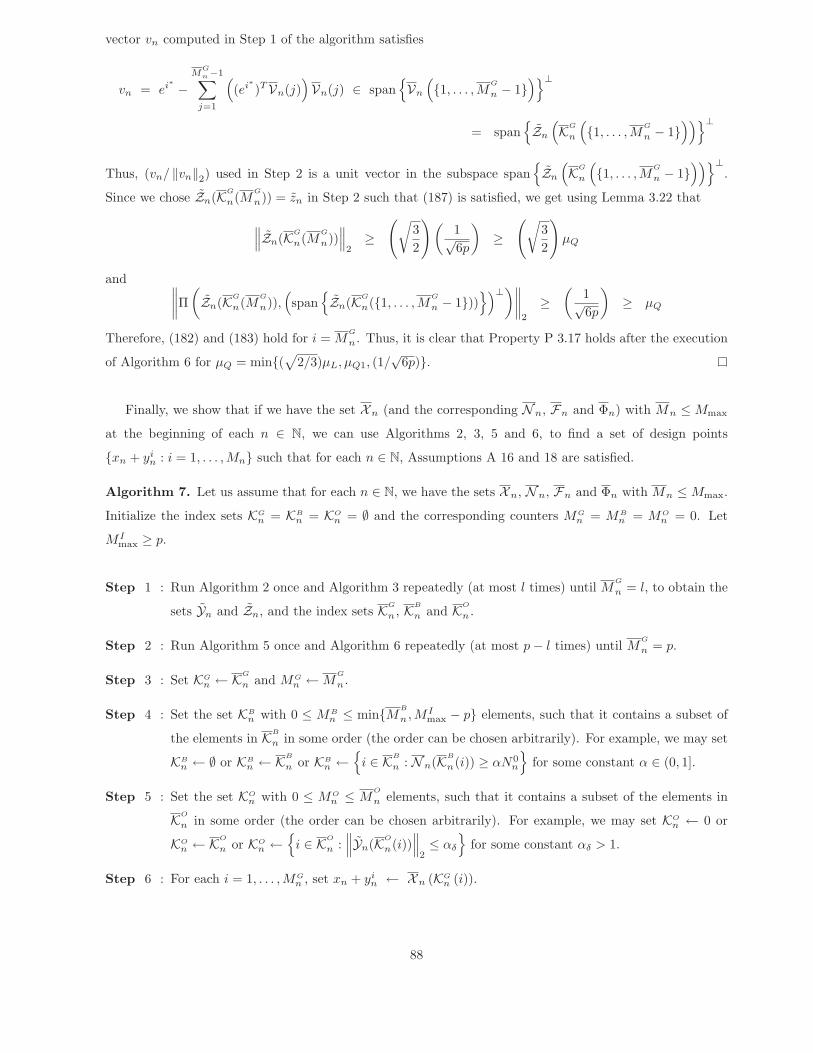
vector vn computed in Step 1 of the algorithm satisfies

vn = ei∗ −M

Gn −1∑

j=1

((ei∗)TVn(j)

)Vn(j) ∈ span

{Vn

({1, . . . ,M

G

n − 1})}⊥

= span{Zn

(KG

n

({1, . . . ,M

G

n − 1}))}⊥

Thus, (vn/ ‖vn‖2) used in Step 2 is a unit vector in the subspace span{Zn

(KG

n

({1, . . . ,M

G

n − 1}))}⊥

.

Since we chose Zn(KG

n(MG

n)) = zn in Step 2 such that (187) is satisfied, we get using Lemma 3.22 that

∥∥∥Zn(KG

n(MG

n))∥∥∥

2≥

(√32

)(1√6p

)≥

(√32

)μQ

and ∥∥∥∥Π(Zn(KG

n(MG

n)),(span

{Zn(KG

n({1, . . . ,MG

n − 1}))})⊥)∥∥∥∥

2

≥(

1√6p

)≥ μQ

Therefore, (182) and (183) hold for i = MG

n . Thus, it is clear that Property P 3.17 holds after the execution

of Algorithm 6 for μQ = min{(√

2/3)μL, μQ1, (1/√

6p)}.

Finally, we show that if we have the set Xn (and the corresponding N n, Fn and Φn) with Mn ≤Mmax

at the beginning of each n ∈ N, we can use Algorithms 2, 3, 5 and 6, to find a set of design points

{xn + yin : i = 1, . . . ,Mn} such that for each n ∈ N, Assumptions A 16 and 18 are satisfied.

Algorithm 7. Let us assume that for each n ∈ N, we have the sets Xn, N n, Fn and Φn with Mn ≤Mmax.

Initialize the index sets KGn = KB

n = KOn = ∅ and the corresponding counters MG

n = MBn = MO

n = 0. Let

M Imax ≥ p.

Step 1 : Run Algorithm 2 once and Algorithm 3 repeatedly (at most l times) until MG

n = l, to obtain the

sets Yn and Zn, and the index sets KG

n , KB

n and KO

n .

Step 2 : Run Algorithm 5 once and Algorithm 6 repeatedly (at most p− l times) until MG

n = p.

Step 3 : Set KGn ← K

G

n and MGn ←M

G

n .

Step 4 : Set the set KBn with 0 ≤ MB

n ≤ min{MB

n ,M Imax − p} elements, such that it contains a subset of

the elements in KB

n in some order (the order can be chosen arbitrarily). For example, we may set

KBn ← ∅ or KB

n ← KB

n or KBn ←

{i ∈ KB

n : Nn(KB

n(i)) ≥ αN0n

}for some constant α ∈ (0, 1].

Step 5 : Set the set KOn with 0 ≤ MO

n ≤ MO

n elements, such that it contains a subset of the elements in

KO

n in some order (the order can be chosen arbitrarily). For example, we may set KOn ← 0 or

KOn ← K

O

n or KOn ←

{i ∈ KO

n :∥∥∥Yn(KO

n(i))∥∥∥

2≤ αδ

}for some constant αδ > 1.

Step 6 : For each i = 1, . . . ,MGn , set xn + yi

n ← Xn (KGn (i)).

88

Step 7 : If MBn > 0, then

• For each i = MGn + 1, . . . , MG

n + MBn , set xn + yi

n ← Xn (KBn (i−MG

n )).

Step 8 : If MOn > 0, then

• For each i = MGn + MB

n + 1, . . . ,MGn + MB

n + MOn , set xn + yi

n ← Xn (KOn (i−MG

n −MBn )).

If Algorithm 7 is run for each n ∈ N, then it is easily seen that the following statements hold.

1. The number of entries in KGn is equal to p and the number of entries in KB

n is at most M Imax− p. Thus,

since Xn(KGn)⋃Xn(KB

n) form the set of inner design points, it is clear that there exist at most M Imax

inner design points for each n ∈ N. Therefore, Assumption A 16 is satisfied for each n ∈ N.

2. From Lemma 3.23, we know that Properties P 3.14, P 3.15 and P 3.17 are satisfied after the execution

of Steps 1 and 2 in Algorithm 7. Thus, from Property P 3.17 we know that the p vectors in Zn(KG

n)

satisfy (182) and (183) and from Property P 3.14, we know that these vectors are the scaled regression

vectors corresponding to the points in Xn(KG

n).

Also, we note from Steps 3 and 6 of Algorithm 7, that the points in Xn(KGn) = Xn(KG

n) are chosen to

be the first p design points. Therefore, from (182) and (183), we get that (160) and (161) are satisfied

by the first p design points and consequently Assumption A 18 is satisfied.

Thus, for each n ∈ N, as long as the design points are chosen using Algorithm 7 and the weights {win :

i = 1, . . . , M In} are chosen so as to satisfy Assumption A 15, we get from (98), (105) and (162) that

(163) holds, i.e. (58) in Assumption A 11 holds with KIλ = (KI

wM Imax/μ2

QSp(μQ)) for each n ∈ N, where

μQ = min{(√

2/3)μL, μQ1, (1/√

6p)}.

Finally, in this section, we consider (35) in Assumption A 7 and (57) in Assumption A 11. In both of

these conditions, we require all the design points {xn + yin : i = 1, . . . ,Mn and n ∈ N} to lie in the compact

set C ⊂ E . Let us see how this can satisfied. Suppose that the following assumption holds.

A 19. There exists a compact set C ⊆ X such that {xn}n∈N⊂ C.

Then, since X ⊂ E , we get that C ⊂ E . Since C is compact and E is open, we get from we get from

Lemma 2.1 in ?, that there exists δ∗ > 0 and a compact set

C :={x = x1 + x2 : x1 ∈ C and

∥∥x2∥∥

2≤ δ∗

}such that C ⊂ E . Now, suppose we choose our design region radii such that δn ≤ δ∗ for each n ∈ N.

Then, it is clear that for each n ∈ N, we have {xn + yin : i = 1, . . . ,M I

n} ⊂ C ⊂ E . Further, note that in

Algorithms 4 and 7, we never evaluate sample averages at new design points that lie outside the design region

89

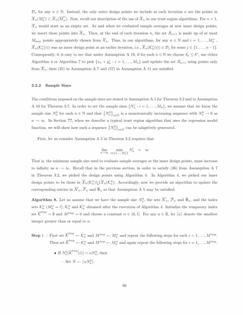
Dn for any n ∈ N. Instead, the only outer design points we include at each iteration n are the points in

Xn(MOn ) ⊂ Xn(M

O

n). Now, recall our description of the use of Xn in our trust region algorithms. For n = 1,

Xn would start as an empty set. As and when we evaluated sample averages at new inner design points,

we insert these points into Xn. Then, at the end of each iteration n, the set Xn+1 is made up of at most

Mmax points appropriately chosen from Xn. Thus, in our algorithms, for any n ∈ N and i = 1, . . . ,MOn ,

Xn(KOn(i)) was an inner design point at an earlier iteration, i.e., Xn(KO

n(i)) ∈ Dj for some j ∈ {1, . . . , n−1}.Consequently, it is easy to see that under Assumption A 19, if for each n ∈ N we choose δn ≤ δ∗, use either

Algorithm 4 or Algorithm 7 to pick {xn + yin : i = 1, . . . ,Mn} and update the set Xn+1 using points only

from Xn, then (35) in Assumption A 7 and (57) in Assumption A 11 are satisfied.

3.2.2 Sample Sizes

The conditions imposed on the sample sizes are stated in Assumption A 5 for Theorem 3.2 and in Assumption

A 10 for Theorem 3.7. In order to set the sample sizes {N in : i = 1, . . . , Mn}, we assume that we know the

sample size N0n for each n ∈ N and that

{N0

n

}n∈N

is a monotonically increasing sequence with N0n → 0 as

n → ∞. In Section ??, when we describe a typical trust region algorithm that uses the regression model

function, we will show how such a sequence{N0

n

}n∈N

can be adaptively generated.

First, let us consider Assumption A 5 in Theorem 3.2 requires that

limn→∞ min

i∈{1,...,MIn}

N in = ∞

That is, the minimum sample size used to evaluate sample averages at the inner design points, must increase

to infinity as n → ∞. Recall that in the previous section, in order to satisfy (36) from Assumption A 7

in Theorem 3.2, we picked the design points using Algorithm 4. In Algorithm 4, we picked our inner

design points to be those in Xn(KGn)⋃Xn(KB

n). Accordingly, now we provide an algorithm to update the

corresponding entries in N n, Fn and Φn so that Assumption A 5 may be satisfied.

Algorithm 8. Let us assume that we have the sample size N0n, the sets Nn, Fn and Φn, and the index

sets KGn (MG

n = l), KBn and KO

n obtained after the execution of Algorithm 4. Initialize the temporary index

set Ktmp= ∅ and M tmp = 0 and choose a constant α ∈ (0, 1]. For any a ∈ R, let �a� denote the smallest

integer greater than or equal to a.

Step 1 : First set Ktmp ← KGn and M tmp ← MG

n and repeat the following steps for each i = 1, . . . ,M tmp.

Then set Ktmp ← KBn and M tmp ←MB

n and again repeat the following steps for i = 1, . . . ,M tmp.

• If N0n(Ktmp

(i)) < αN0n, then

– Set N ← �αN0n�.

90

– If Nn(Ktmp(i)) > 0, then compute f(Xn(Ktmp

(i)), N) using Fn(Ktmp(i)) in (164) and

σ(Xn(Ktmp(i)), N) usingN n(Ktmp

(i)), Fn(Ktmp(i)), f(Xn(Ktmp

(i)), N) and Φn(Ktmp(i))

in (170).

– If Nn(Ktmp(i)) = 0, then compute f(Xn(Ktmp

(i)), N) and σ(Xn(Ktmp(i)), N) using (8)

and (169) respectively.

– SetN n(Ktmp(i))← N , Fn(Ktmp

(i))← f(Xn(Ktmp(i)), N) and Φn(Ktmp

(i))← σ(Xn(Ktmp(i)), N).

Step 2 : Set N in ← Nn(KG

n(i)) for each i = 1, . . . ,MGn .

Step 3 : If MBn > 0, set N i

n ← Nn(KBn(i−MG

n )) for each i = MGn + 1, . . . ,MG

n + MBn .

Step 4 : If MOn > 0, set N i

n ← N n(KOn(i−MG

n −MBn )) for each i = MG

n + MBn + 1, . . . , MG

n + MBn + MO

n .

For each n ∈ N, upon execution of Algorithm 8, it is easily seen that N in ≥ αN0

n for each i = 1, . . . ,M In.

Therefore, if we ensure that N0n →∞ as n→∞, then clearly Assumption A 5 is satisfied.

Next, in order to satisfy Assumption A 10, we have to set N in = N#

n for each i = 1, . . . , Mn and n ∈ N,

where N#n →∞ as n→∞. In the previous section, we used Algorithm 7 to pick the design points so as to

satisfy (58) from Assumption A 11 in Theorem 3.7. Recall that upon execution of Algorithm 7, the inner

design points were set to be those in Xn(KGn)⋃Xn(KB

n), and the outer design points were those in Xn(KOn).

Therefore, we will provide an algorithm next that updates the corresponding elements of Nn, Fn and Φn.

Algorithm 9. Let us assume that we have the sample size N0n, the sets Nn, Fn and Φn, and the index

sets KGn (MG

n = l), KBn and KO

n obtained after the execution of Algorithm 7. Initialize the temporary index

set Ktmp= ∅ and M tmp = 0 and choose a constant α ∈ (0, 1]. For any a ∈ R, let �a� denote the smallest

integer greater than or equal to a.

Step 1 : Set

N#n ← max

{�αN0

n�,max{N n(k) : k ∈ KG

n

⋃KB

n

⋃KO

n

}}

Step 2 : First set Ktmp ← KGn and M tmp ← MG

n and repeat the following steps for each i = 1, . . . ,M tmp.

Then set Ktmp ← KBn and M tmp ← MB

n and again repeat these steps for each i = 1, . . . ,M tmp.

Finally set Ktmp ← KOn and M tmp ←MO

n and repeat these steps for each i = 1, . . . ,M tmp.

• If N0n(Ktmp

(i)) < N#n , then

– Set N#n ← �αN0

n�.

– If N n(Ktmp(i)) > 0, then compute f(Xn(Ktmp

(i)), N#n ) using Fn(Ktmp

(i)) in (164)

and σ(Xn(Ktmp(i)), N#

n ) using Nn(Ktmp(i)), Fn(Ktmp

(i)), f(Xn(Ktmp(i)), N#

n ) and

Φn(Ktmp(i)) in (170).

91

– If N n(Ktmp(i)) = 0, then compute f(Xn(Ktmp

(i)), N#n ) and σ(Xn(Ktmp

(i)), N#n ) using

(8) and (169) respectively.

– Set Nn(Ktmp(i)) ← N#

n , Fn(Ktmp(i)) ← f(Xn(Ktmp

(i)), N#n ) and Φn(Ktmp

(i)) ←σ(Xn(Ktmp

(i)), N#n ).

Step 3 : Set N in ← Nn(KG

n(i)) for each i = 1, . . . ,MGn .

Step 4 : If MBn > 0, set N i

n ← Nn(KBn(i−MG

n )) for each i = MGn + 1, . . . ,MG

n + MBn .

Step 5 : If MOn > 0, set N i

n ← N n(KOn(i−MG

n −MBn )) for each i = MG

n + MBn + 1, . . . , MG

n + MBn + MO

n .

From the definition of N#n in Step 1 of the above algorithm, it is clear that before the execution of Step

2, Nn(k) ≤ N#n for each k ∈ KG

n

⋃KB

n

⋃KO

n . Thus for each n ∈ N, upon termination of the algorithm, we

clearly get that N in = N#

n ≥ αN0n for each i = 1, . . . ,Mn. Consequently, since we ensure the N0

n → ∞ as

n→∞, if we run Algorithm 9 for each n ∈ N, then Assumption A 10 is satisfied.

3.2.3 Weights

In this section we consider methods to set the weights {win : i = 1, . . . ,Mn} for each n ∈ N. Note that the

weight matrices corresponding to the inner and outer design points, specified in the matrices W In and WO

n

respectively, occur in (36) and (37) in Assumption A 7 and (58) and (59) in Assumption A 11. We already

showed in Section 3.2.1, how the design points may picked for each n ∈ N, so as to satisfy (36) and (58),

using Assumption A 15. Here, we provide methods to pick the weights {win : i = 1, . . . , Mn} for each n ∈ N

such that the conditions (37) in Assumption A 7, (59) in Assumption A 11 and also Assumption A 15 may

be satisfied.

The intuition behind the two conditions in ((37) and (59)) is as follows. As we mentioned earlier, we

introduced the design region Dn for each iteration n, in order to be able to control the Euclidean distances∥∥yin

∥∥2

of the design points xn +yin from the iterate xn. Indeed we could, if we wanted, use only points within

the design region Dn to determine ∇nf(xn) and ∇2nf(xn) for each n ∈ N. However, as our optimization

algorithm progresses, it is likely that some points in the set Xn (i.e., points at which sample averages have

been evaluated in earlier iterations), will lie outside the design region Dn for iteration n. Since we have

already evaluated sample averages at these points, we wish to include these points in the determination of

mn. However, in order for ∇nf(xn) to better approximate ∇f(xn), it is also true that the inner design points

must provide progressively higher contributions to the determination ∇nf(xn) and ∇2nf(xn) as compared

to the outer design points . Thus, the conditions (37) and (59), balance these two conflicting requirements

by requiring that the outer design points , be assigned progressively smaller weights {wMIn+1

n , . . . , wMnn } as

n → ∞, when compared to the weights {w1n, . . . , w

MIn

n } assigned to inner design points. Essentially these

92

conditions ensure that as n→∞, the outer design points are ignored and only the points within the design

region are used to calculate ∇nf(xn) and ∇2nf(xn).

Consider the following method for setting the weights {win : i = 1, . . . ,Mn}.

Algorithm 10. Let us suppose that the design points {xn + yin : i = 1, . . . , Mn} are available to us. Let

r ∈ R be a positive constant.

Step 1 : Define πn ← mini∈{1,...,MIn}∥∥yi

n

∥∥2

Step 2 : Set for each i = 1, . . . , Mn,

win ←

⎧⎪⎨⎪⎩

1 for i ∈{1, . . . , M I

n

}(

π2n

‖yin‖2

2

)min {1, (δn)r} for i ∈

{M I

n + 1, . . . ,Mn

} (190)

Algorithm 10 warrants the following comments.

• In order for (190) to be well-defined, we must have∥∥yi

n

∥∥2

> 0 for each i = M In + 1, . . . ,Mn. From our

convention since {xn + yin : i = M I

n + 1, . . . ,Mn} is the set of outer design points, we have∥∥yi

n

∥∥2

> δn

for each i = M In + 1,Mn. Therefore, as long as δn > 0, Algorithm 10 is well defined.

• It is easily seen that in the above example, win < 1 for each i = M I

n + 1, . . . ,Mn and n ∈ N. Thus,

the outer design points always get a lower weight as compared to the inner design points. Further, it

is easy to see that if δn → 0 as n→∞, then the weights given to the outer design points decrease to

zero as n→∞.

Lemma 3.24. Let the following assumptions hold.

1. The sequence {δn}n∈Nof design region radii satisfies δn → 0 as n→∞.

2. There exists a constant MDmax <∞, such that 1 ≤M I

n ≤Mn ≤MDmax. for each n ∈ N.

Then, if the weights {win : i = 1, . . . ,Mn} are assigned using Algorithm 10 for each n ∈ N, (37) in Assumption

A 7 is satisfied for any r > 0.

Further, if there exists Ky < ∞ such that∥∥yi

n

∥∥2

< Ky for all i = 1, . . . ,Mn and n ∈ N, then (59) in

Assumption A 11 is satisfied for any r > 2.

Proof. First, let us consider (37). It is not hard to see that∥∥∥(Y On )T WO

n Y On

∥∥∥2∥∥∥(Y I

n )T W In Y I

n

∥∥∥2

=

∥∥(Y On )T WO

n Y On

∥∥2

‖(Y In )T W I

nY In ‖2

≤ l

(trace(Y O

nTWO

n Y On )

trace(Y In

TW I

nY In )

)= l

⎛⎝∑Mn

i=MIn+1 wi

n

∥∥yin

∥∥2

2∑MIn

i=1 win ‖yi

n‖22

⎞⎠

93

Substituting the weights mentioned in (190) into the above and manipulating the resulting expressions, we

get ∥∥∥(Y On )T WO

n Y On

∥∥∥2∥∥∥(Y I

n )T W In Y I

n

∥∥∥2

≤ l

(min{1, (δn)r}π2

n(Mn −M In)∑MI

ni=1 ‖yi

n‖22

)≤ l

(min{1, (δn)r}(Mn −M I

n)M I

n

)

We know that MDmax ≥ Mn ≥ M I

n ≥ 1 for each n ∈ N. Therefore, ((Mn −M In)/M I

n) ≤ 2MDmax. Further,

since δn → 0 as n→∞ and r > 0, we finally get

limn→∞

∥∥∥(Y On )T WO

n Y On

∥∥∥2∥∥∥(Y I

n )T W In Y I

n

∥∥∥2

≤ 2l (MD

max) limn→∞min {1, (δn)r} = 0

Thus, (37) in Assumption 7 is satisfied.

Next, assuming in addition, that∥∥yi

n

∥∥2

< Ky for all i = 1, . . . ,Mn and n ∈ N, consider (59). It is easily

seen that ∥∥∥(ZOn )T WO

n ZOn

∥∥∥2∥∥∥(ZI

n)T W In ZI

n

∥∥∥2

≤ p

⎛⎝∑Mn

i=MIn+1 wi

n

∥∥zin

∥∥2

2∑MIn

i=1 win ‖zi

n‖22

⎞⎠

Now, substituting the weight distribution from (190) into the numerator of the above expression and using

the definition of zin, we get

Mn∑i=MI

n+1

win

∥∥zin

∥∥2

2=

Mn∑i=MI

n+1

min{1, (δn)r}(

π2n

‖yin‖

22

)∥∥zin

∥∥2

2≤

Mn∑i=MI

n+1

(δn)r

(π2

n

‖yin‖

22

)(∥∥yin

∥∥2

2

δ2n

+

∥∥yin

∥∥4

2

2δ4n

)

≤Mn∑

i=MIn+1

(δn)(r−2)π2n

(1 +

∥∥yin

∥∥2

2

2δ2n

)(191)

Also, we haveMI

n∑i=1

win

∥∥zin

∥∥2

2=

MIn∑

i=1

(∥∥yin

∥∥2

2

δ2n

+

∥∥yin

∥∥4

2

2δ4n

)≥

MIn∑

i=1

(∥∥yin

∥∥2

2

δ2n

)(192)

Thus, combining (191) and (192) and noting that∥∥yi

n

∥∥2

< Ky for all i = 1, . . . , Mn and n ∈ N, we have

∑Mn

i=MIn+1 wi

n

∥∥zin

∥∥2

2∑MIn

i=1 win ‖zi

n‖22

≤

∑Mn

i=MIn+1(δn)(r−2)π2

n

(1 +‖yi

n‖222δ2

n

)∑MI

ni=1

(‖yin‖2

2δ2

n

) ≤(δn)(r−2)

(δ2n + K2

y

2

)(Mn −M I

n)∑MIn

i=1

(‖yin‖2

2π2

n

)≤ (δn)(r−2)

(δ2n +

K2y

2

)(Mn −M I

n

M In

)(193)

As before, since ((Mn −M In)/M I

n) ≤ 2MDmax, δn → 0 as n→ 0 and r > 2, we get

limn→∞

∑Mn

i=MIn+1 wi

n

∥∥zin

∥∥2

2∑MIn

i=1 win ‖zi

n‖22

≤ 2MD

max limn→∞(δn)(r−2)

(δ2n +

K2y

2

)= 0

Thus, we finally get that

limn→∞

∥∥∥(ZOn )T WO

n ZOn

∥∥∥2∥∥∥(ZI

n)T W In ZI

n

∥∥∥2

≤ p limn→∞

⎛⎝∑Mn

i=MIn+1 wi

n

∥∥zin

∥∥2

2∑MIn

i=1 win ‖zi

n‖22

⎞⎠ = 0

94

Note the following regarding the assumptions of Lemma 3.24.

1. Suppose we pick our design points {xn + yin : i = 1, . . . ,Mn} for each n ∈ N using either Algorithm 4

or 7. Then for each n ∈ N, we note that before either of these algorithms are executed, we know that

the number of entries in Xn is at most Mmax. In either Algorithm 4 we add at most l points into Xn,

and in Algorithm 7 we add at most p new points in to Xn. Therefore, in either case, it is easily seen

that l ≤M In ≤Mn ≤Mmax + p.

2. Further, it is easily seen that if there exists a compact set C ⊂ E such that xn + yin ∈ C for each n ∈ N

and i = 1, . . . ,Mn, then there exists Ky <∞ such that∥∥yi

n

∥∥2

< Ky for each n ∈ N and i = 1, . . . , Mn

Finally it is also clear that if the weights {win : i = 1, . . . , M I

n} corresponding to the inner design points,

are picked as in Algorithm 10, then

min{win : i = 1, . . . , M I

n} = max{win : i = 1, . . . , M I

n} = 1

Therefore, in this case Assumption A 15 used in Section 3.2.1 is satisfied with KIw = 1.

95

Derivative Free Trust Region Algorithms for Stochastic Optimizationanton/truststoch3.pdf ·...

Documents

Transcript of Derivative Free Trust Region Algorithms for Stochastic Optimizationanton/truststoch3.pdf ·...