A Mushy Region in Concrete Corrosion

C. V. Nikolopoulos

Department of Mathematics, University of the Aegean,Karlovasi, 83200, Samos, Greece.

Abstract

In this work a mathematical model already known for the corrosion of sewer pipes isfurther considered, enriched and an approximate analytical solution is given basedon a quasi steady approximation. Furthermore an extension of this model is con-structed allowing the formation of a mushy region, i.e. a region in which the ma-terial is only partly corroded throughout the process. This more general model isderived via an averaging process by microscopic considerations and has the form of amacroscopic phase field model. The derived model in its various forms is solved nu-merically with a finite element method and the results, predicting corrosion withina reasonable range, are presented.

Key words: Sulfide Corrosion, Concrete Corrosion, Free Boundary Problems,Perturbation methods.

1 Introduction

A model regarding transport of sewage in sewer pipes which leads to the releaseof hydrogen sulfide (H2S) and reacts to form a corrosive compound (H2SO4)in sewers is considered in [4]. More specifically, in [4], biological generation ofSO−

4 from H2S and transport of H2S and SO−4 from the interior of the pipe

to the corrosion front separating corroded and uncorroded parts of the pipewalls, is modelled by a system of three weakly coupled reaction - diffusionequations. The model is presented initially in [4] and it is also studied in [5].Existence and uniquiness of the system is studied in [12]. Some experimentalresults regarding corrosion of sewer pipes are also presented in [3].

The basic reaction that it is considered, expressing the actual fact that H2SO4

reacts with calsite CaCO3 forming gypsum CaSO4 · 2H2O and causing the

Email address: cnikolo@aegean.gr (C. V. Nikolopoulos).

Preprint submitted to Elsevier 30 March 2010

corrosion of the concrete, is the following:

2H2O + H+ + SO2−4 + CaCO3

Kc−→ CaSO4 · 2H2O + HCO−3 .

As it is also addressed in [4] a model considering the formation of a mushyregion should be useful, giving a more realistic approach to the phenomenon. Amushy region in this case would mean to have both uncorroded and corrodedparts of the material coexisting during the process in an element volume of itand not having a distinct macroscopic interface separating the corroded anduncorroded parts of the material.

Note that the aforementioned chemical reaction is the same when we considerfor example corrosion due to H2S of marble of antiquities or of similar physi-cal systems. More specifically a series of studies for the chemical aggregationof limestones (corrosion of antiquities), which in its basis it is a similar phe-nomenon, has been presented in a series of papers as in [1], [2], [8], [9], [10].With minor modifications the models derived in this work can also be adoptedin the case that we study corrosion of marbles from atmospheric pollution orother physical systems as well (see [9] etc.). Note that in these models it isassumed a linear dependence of the porosity from the calcite concentrationwhile in the present work the dependence of the porosity from the calcite con-centration comes from a differential equation which is derived from specificconsiderations for the microstructure of the system.

In the present work as an example of a physical system, illustrating how amodel which accounts for the formation of a mushy region can be derived,we will use as a base the model derived in [4]. Initially, in Section 2, we willpresent it and give a brief explanation of how the equations of the modelare derived. Then we apply a nondimensionalization to simplify the set ofequations and in order to have an overview of the behaviour of the solutionof the equation, additional to the results presented in [4], we apply the quasisteady approximation (omitted in [4]) to give an analytical approximation ofthe solution for some suitable range of the parameters of the model.

Having already some overview of this initial model we then apply the methodof multiple scales to construct a phase field model derived from microstructureconsiderations in Section 3. This is motivated by a method initially presentedin [13] and [14] which is adopted and modified appropriately to analyze theproblem in our case. In order to do that we will consider inside the concreteand in the microstructure scale, cracks being parallel between them (in oneand two - dimensional consideration) and equally spaced. The derived phasefield models are presented in Section 3. In Section 4 the basic equation derivedis solved numerically via a finite element method. The same method is appliedto solve numerically the corresponding system of equations in the case that we

2

study the corrosion of the sewer pipes. This is also done for the case that thissystem is simplified with the use of the quasi steady approximation. Finallythe conclusions of this work are presented in Section 5.

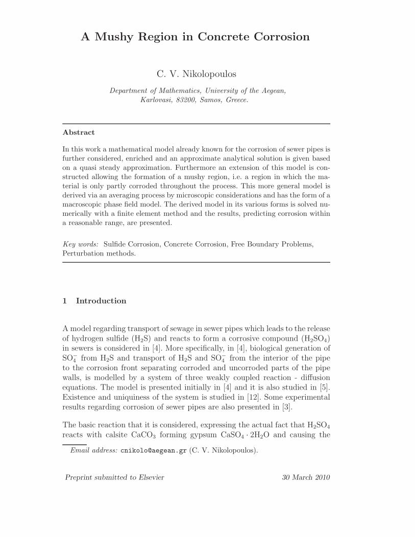
a(t) x=0 s(t) x=l

GYPSUM CONCRETE

Fig. 1. Schematic representation of a sewer pipe corrosion

2 Presentation of the model and the Quasi Steady Approximation

The governing chemical reactions leading to the corrosion of sewer pipes (see[4]) are the following:

10H+ + SO2−4 +org. matter −→H2S + 4H2O+oxidized org. matter

H2S + 2O2KB−→ 2H+ + SO2−

4

2H2O + H+ + SO2−4 + CaCO3

Kc−→ CaSO4 · 2H2O + HCO−3 .

We denote by u, v and w the concentrations of H2S in the gaseous phase, ofH2S in the liquid phase and of SO2−

4 respectively, i.e. u := [H2S]g, v := [H2S]aqand w := [SO2−

4 ], where [ · ] denotes the concentration, the subscript g thegaseous phase, while the subscript aq stands for water. The constants KB andKc are the bio-conversion rate constant and the constant of reaction (disso-lution rate constant) respectively (see [4]). The gypsum - concrete interfaceis represented by x = s(t), for x measuring distance from the inner side ofthe wall and it is a nondecreasing function of time representing the progressof the corrosion inside the concrete. Also we may consider a second moving

3

boundary determining the motion of the outer surface of the material which isbeing corroded, denoted by a(t), with a(0)=0 and which expresses the expan-sion of volume of the concrete-gypsum system, coming from the fact that theformed gypsum has lower density than the concrete. Now if we consider a one- dimensional movement of the corrosion front and if Ω(t) = (a(t), s(t)), theinterval which determines the corroded part of the material i.e. the gypsumpart, then the equations for u, v and w are the following (see [4])

ut = Dauxx + Pu,

vt = Dwvxx + Pv1+ Pv2

,

wt = DHwxx + Pw1+ Pw2

.

with

u(a(t), t) = λ1, ux(s(t), t) = 0,

v(a(t), t) = λ2, vx(s(t), t) = 0,

w(a(t), t) = λ3, DHwx(s(t), t) + Kc (w(s(t), t))m = 0.

where Da, Dw, DH are the diffusion coefficients and Pu, Pv1, Pv2

, Pw1, Pw2

arevarious source terms which will be specified in the following. There is also needfor the moving boundaries a(t), and s(t) to be specified by some additionalequations which also will be given in the following. In addition we assumeDirichlet boundary conditions at the one end, a(t) and Neumann conditionsat the moving boundary s(t), except for w where we have that the flow of wsupplies with material the chemical reaction which transforms concrete intogypsum so that a condition of Robin type is posed instead. Actually the Robinboundary condition follow from the assumption that the calcite to gypsumreaction will go to completion whenever there is a non-negligible consentrationof sulphate ions (fast reaction) and therefore we can consider that the reactionis happening at the surface separating calcite from gypsum.

As an initial approximation we may take a(t) = 0, for t ≥ 0 accounting for thefact that the volume expansion of the material, due to the corrosion process,is negligible. Note also that regarding the diffusivities we have Da = TaVaDha,Dw = TaVwDhw, DH = TaVwDsaw where Va, Vw are the porosities of the air andthe water filled regions respectively, Da, Dw, Dsaw are the diffusion rates foru, v and w respectively and Ta is the tortuosity. We then focus our attentionon the source terms. The term Pu expresses the exchange of H2S between theair and the water phase, i.e.

4

Pu = −KT AS

Va

(KHSu − v),

whereKT is the mass transfer coefficient,AS is the surface area,Va is the porosity, fraction of volume of air filled pores,KHS is the Henry’s law constant.

The term Pv1, similarly, expresses the exchange of H2S between the water and

the air phase (inverse process of the one expressed by Pu), i.e.

Pv1=

KT AS

Vw

(KHSu − v),

whereVw is the porosity, fraction of volume of water filled pores.In addition the term Pv2

expresses the bioconversion of H2S, that is,

Pv2= −KBv.

Also in the equation for w we have that Pw1= −Pv2

, i.e. H2S is giving SO2−4

due to bioconversion and the term Pw2expresses absorption of H2S due to

reaction with residues of CaCO3 in water filled pores. In such a case we have

Pw2= −Kcw

mCnc ,

for Cc being the concentration of calcite, Kc the reaction constant and m, nthe orders of the reactions.

If we assume that the reaction is complete at the boundary we have Pw2= 0,

i.e. no CaCO3 is left after the reaction.

In the following we will therefore use the assumption that Pw2= 0 where

w > 0.

Therefore the resulting set of equations has the form

ut = Dauxx −KT AS

Va

(KHSu − v), (2.1a)

5

vt = Dwvxx +KT AS

Vw

(KHSu − v) − KBv, (2.1b)

wt = DHwxx + KBv. (2.1c)

The boundary conditions at x = 0, at x = s(t) and the Stefan condition havethe form

u(0, t) = λ1, v(0, t) = λ2, w(0, t) = λ3, (2.2a)

ux(s(t), t) = 0, vx(s(t), t) = 0, Kc (w(s(t), t))m + DHwx(s(t), t) = 0, (2.2b)

s(t) =Kc

Cc

wm, (2.2c)

where Kc is the constant of reaction and m the reaction rate. Furthermoreequation (2.2c) can be derived (see also [4]) by considering that Ccs(t) standsfor the amount of calcium carbonate consumed per unit time which equals thereaction rate and thus Ccs(t) = Kcw

m or s = −Pw2for n = −1. Also λ1, λ2, λ3

are the given concentrations at x = 0.

These equations can be modified by dropping some of the assumptions we haveadopted. More specifically in the case that we drop the assumptions regardingthe outer free boundary a(t) and the one regarding the source term Pw2

bytaking a(t) 6= 0 and Pw2

6= 0, the system takes the form of equations (2.1a),(2.1a) with the equation of w having the form

wt = DHwxx + KBv − KcwmCn

c , (2.3)

and with the addition also of an equation for the calcite variation. Possibleconvective terms resulting from the expansion of the material, i.e. from al-lowing a(t) < 0 can also be included in the equations for the concentrations.Although in this work when a(t) 6= 0 such terms will be considered negligibleand not be taken into account (see also [4]).

In addition to the fact that we may take a(t) 6= 0 and Pw26= 0 it is worth noting

that also we can impose Robin boundary conditions at the left boundary , i.e.

ux(a(t), t) = Eup(u − λ1(t)), (2.4a)

vx(a(t), t) = Evl(u − λ2(t)), (2.4b)

wx(a(t), t) = Ewl(w − λ3(t)), (2.4c)

where Eup, Erl, Ewl, are the mass transfer coefficients. In the rest of this workwe will not consider these conditions in equation (2.4) and (2.3) and we willalways assume Dirichlet conditions at the left boundary and that the reactionat the moving boundary is complete giving Pw2

= 0. Although the relevantanalysis can be easily modified to include equation (2.4) instead of (2.2a) orthe source term in equation (2.3).

Regarding now the a(t) 6= 0 case, at x = s(t) we have similarly as beforethe boundary conditions to be given by the equations (2.2b), (2.2c) and thepropagation of a(t) to be given by the relation

6

a(t) =

(

1 − ρc

ρg

)

kc

Cc

w(s(t), t)m, (2.5)

for ρc and ρg being the densities of the calcite and the gypsum respectively.This comes by a direct application of a conversation law (see [4]). In casethat we take ρc 6= ρg, i.e. the calcium and the gypsum density to differ, we

have ρcs(t) = ρg

(

s(t)− a(t))

and equation (2.5) is implied. Moreover as initial

conditions for both cases (for a = 0 or a 6= 0) in order to complete the systemof equations, we may take

u(x, 0) = 0, v(x, 0) = 0, w(x, 0) = 0. (2.6)

Finally in the following and in the rest of this work, for simplicity reasons, wewill assume as in [4] that m = 1 .

Nondimensionalization We focus our attention to the system of equations(2.1), (2.2), (2.6) and we scale the problem by the use of appropriate constants.We scale x with l, y = x

lwhere l is a typical length of the observed corrosion

in a period of years. Also we scale u, v, w with λ1, λ2, λ3 respectively and wehave

U =u1

λ1, V =

v

λ2, W =

w

λ3, S =

s

l.

In addition we set τ = tt0

for τ being the dimensional variable and for t0a typical time which will be chosen in such a way so that the terms in theequation of the moving boundary are balanced.

Therefore the equation for u becomes

(

l2

Dat0

)

∂U

∂τ=

∂2U

∂y2−(

KT Asλ2

Vaλ1

l2

Da

)(

KHSλ1

λ2

U − V

)

,

or

ε1∂U

∂τ=

∂2U

∂y2− µ1 (β1U − V ) , 0 < y < S(τ),

for ε1 = l2

Dat0, µ1 = KT Asλ2l2

Vaλ1Daand β1 = KHSλ1

λ2. Note that β1 = 1 due to the fact

that KHSλ1 = λ2 for numbers given in [4].

7

In a similar way we deduce that

ε2∂V

∂τ=

∂2V

∂y2+ µ2 (U − V ) − β2V, 0 < y < S(τ),

for ε2 = l2

Dwt0, µ2 = KT Asl2

VwDwand β2 = kB l2

Dw, and that

ε3∂W

∂τ=

∂2W

∂y2+ β3V, 0 < y < S(τ),

for ε3 = l2

DH t0, and β3 = kBλ2l2

DHλ3.

Regarding the boundary conditions at x = 0 we have

U(0, t) = V (0, t) = W (0, t) = 1, y ∈ (0, S(0)).

The boundary conditions at y = S(τ) now have the form

Uy(S(τ), τ) = 0, Vy(S(τ), τ) = 0, γWy(S(τ), τ) + W (S(τ), τ) = 0,

for γ = DH

lKc.

Finally the equation for S(τ) becomes

S(τ) = W (S(τ), τ),

for the appropriate choice of t0, given by t0 = CclKcλ3

.

Summarizing we have the system

ε1∂U

∂τ=

∂2U

∂y2− µ1 (U − V ) , (2.7a)

ε2∂V

∂τ=

∂2V

∂y2+ µ2 (U − V ) − β2V, (2.7b)

ε3∂W

∂τ=

∂2W

∂y2+ β3V (2.7c)

for 0 < y < S(τ), with boundary conditions,

U(0, τ) = 1, Uy(S(τ), τ) = 0, (2.8a)

V (0, τ) = 1, Vy(S(τ), τ) = 0, (2.8b)

8

W (0, τ) = 1, γWy(S(τ), τ) + W (S(τ), τ) = 0, (2.8c)

the condition for the free boundary,

S(τ) = W (S(τ), τ), S(0) = Sa, (2.9)

for τ > 0, some Sa > 0 and the initial conditions

U(y, 0) = 0, V (y, 0) = 0, W (y, 0) = 0, 0 < y < S(0). (2.10)

Taking numbers by [4] we have for example that for Kc = 0.0084, l = 2 cmand the D′

is, KT , As, V′i s, KB etc. taken as in [4] that ε1 ' O(10−7), ε2, ε3 '

O(10−3), while µ1 ' 7.57×105, µ2 ' 3.03×109 and β2 ' 2.52×103, β3 ' 0.025,γ ' 6.78.

These sizes justify the use of the quasi-steady approximation for the problem.Note that this approximation would be useful in general for values of theparameters giving the ε′s small and negligible in the set of equations (2.7). Inother words it seems that for this physical system, for a time scale of yearswhere the evolution of corrosion is observable, we have very fast diffusiontogether with very fast exchange of H2S between the air and water filledpores. Indeed for ε1, ε2, ε3 1, µ1, µ2 1, β2 1, we rewrite the equationsin the following form

ε1

µ1

∂U

∂τ=

1

µ1

∂2U

∂y2− (U − V ) ,

ε2

µ2

∂V

∂τ=

1

µ2

∂2V

∂y2+ (U − V ) − β2

µ2

V,

ε3∂W

∂τ=

∂2W

∂y2+ β3V,

with the initial and boundary conditions given by equations (2.8), (2.9) and(2.10). We notice that β2

µ2= O( 1

µ1) so we can set for some ν2 ' O(1) that

β2

µ2= ν2

1µ1

.

We also set ε = 1√µ2

and ν1ε = 1µ1

for ν1 = O(1). Thus we obtain

9

ε1εν1∂U

∂τ= εν1

∂2U

∂y2− (U − V ) ,

ε2ε2 ∂V

∂τ= ε2∂2V

∂y2+ (U − V ) − ν2ν1εV,

ε3∂W

∂τ=

∂2W

∂y2+ β3V.

Note that, motivated by the numbers given in [4], we may take ε1 ' O(ε2)and ε2, ε3 ' O(ε). Therefore we may take an expansion of the form

U ∼U0 + εU1 + ε2U2 + . . . ,

V ∼V0 + εV1 + ε2V2 + . . . ,

W ∼W0 + εW1 + ε2W2 + . . . ,

S ∼S0 + εS1 + ε2S2 + . . . ,

and substituting these expressions for U and V to the relevant equations weget

ε1εν1 (U0τ + εU1τ + . . .) = ν1ε(

U0yy + εU1yy + . . .)

− (U0 − V0)

−ε (U1 − V1) − . . . , (2.11)

ε2ε2 (V0τ + εV1τ + . . .) = ε2

(

V0yy + εV1yy + . . .)

+ (U0 − V0) + ε (U1 − V1)

−ν1ν2εV0 − ν1ν2ε2V1 − . . . , (2.12)

ε3 (W0τ + εW1τ + . . .) =(

W0yy + εW1yy + . . .)

+ β3V0 + β3εV1 + . . . . (2.13)

By equations (2.11) and (2.12) we obtain to O(1) terms that

U0 − V0 = 0.

Also by the fact that ε3 = O(ε) 1 and by equation (2.13) we obtain to O(1)terms

10

W0yy + β3V0 = 0. (2.14)

Looking at the O(ε) terms we get by equations (2.11) and (2.12) that

ν1U0yy − (U1 − V1)= 0,

(U1 − V1) − ν1ν2V0 = 0.

Thus we get U1 − V1 = ν1ν2V0 and as a consequence that

U0yy − ν2V0 = 0,

or that

U0yy − ν2U0 = 0, with U(0, τ) = 1, Uy(S0(τ), τ) = 0.

This implies that the solution for U0 is

U0(y, τ) = U0(y; S0(τ)) =cosh

(√ν2(y − S0(τ))

)

cosh(√

ν2S0(τ)) ,

and

U0(y, τ) = V0(y, τ).

Now regarding the dominant term in the expansion for W we have

W0yy − β3V0 = 0,

with boundary conditions, to leading order terms,

W0(0, τ) = 1, γW0y(S0(τ), τ) + W0(S0(τ), τ) = 0.

In addition we also have

11

S0(τ) = W0(S0(τ), τ).

Then the solution for W0 is

W0(y, τ)=ν2 + β3

ν2(S0(τ) + γ)[S0(τ) − y + γ]

+β3

ν2(S0(τ) + γ)[y − (S0(τ) + γ)sech (

√ν2(S0(τ) − y))] sech (

√ν2S0(τ)) .

More specifically for y = S(τ) ' S0(τ) we get

W0(S0(τ), τ) =γ(ν2 + β3) − β3γ sech

(√ν2S0(τ)

)

ν2(S0(τ) + γ),

and the resulting equation for S to leading order terms has the form of anordinary differential equation. Indeed we obtain that

dS(τ)

dτ=

γ(ν2 + β3) − β3γ sech(√

ν2S(τ))

ν2(S(τ) + γ), (2.15)

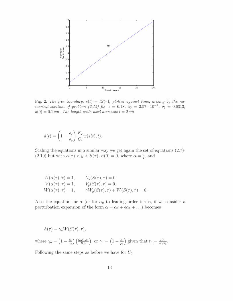
with S(0) = Sa. This equation can be solved easily numerically e.g. via aRunge-Kutta scheme, and in Figure (2) we can see the motion of the movingboundary. The result is in very good agreement with the relevant result in[4] which is produced by the numerical solution via a finite element methodapplied to the full problem and for the value Kc = 0.0084 cm/day.

Case of α(τ) 6= 0. If we assume that a(τ) 6= 0 we have again the previousset of equations, (2.7), (2.8), and (2.10), with the difference that instead ofequation (2.9) at x = 0, we have at x = a(t), boundary conditions having theform

u(a(t), t) = λ1, v(a(t), t) = λ2, u(a(t), t) = λ3,

and also an additional equation for the evolution of a(t) is added (see [4]), i.e.

12

0 5 10 15 20 250

0.2

0.4

0.6

0.8

1

1.2

1.4

1.6

1.8

2

Time in Years

Cor

rosi

onD

epth

in c

m

s(t)

Fig. 2. The free boundary, s(t) = lS(τ), plotted against time, arising by the nu-merical solution of problem (2.15) for γ = 6.78, β3 = 2.57 · 10−2, ν2 = 0.6313,s(0) = 0.1 cm. The length scale used here was l = 2 cm.

a(t) =

(

1 − ρc

ρg

)

Kc

Cc

w(s(t), t).

Scaling the equations in a similar way we get again the set of equations (2.7)-(2.10) but with α(τ) < y < S(τ), α(0) = 0, where α = a

l, and

U(α(τ), τ) = 1, Uy(S(τ), τ) = 0,

V (α(τ), τ) = 1, Vy(S(τ), τ) = 0,

W (α(τ), τ) = 1, γWy(S(τ), τ) + W (S(τ), τ) = 0.

Also the equation for α (or for α0 to leading order terms, if we consider aperturbation expansion of the form α = α0 + εα1 + . . .) becomes

α(τ) = γaW (S(τ), τ),

where γa =(

1 − ρc

ρg

) (

t0Kcλ3

lCc

)

, or γa =(

1 − ρc

ρg

)

given that t0 = lCc

Kcλ3.

Following the same steps as before we have for U0

13

U0yy − ν2U0 = 0,

U(α0(τ), τ) = 1, Uy(S0(τ), τ) = 0.

This results in the expression, for U0 ' V0,

U0(y, τ) = U0(y; S0(τ)) =cosh

(√ν2(S0(τ) − y)

)

cosh(√

ν2(α0(τ) − S0(τ))) .

In addition W0 which satisfies the equation

W0yy − β3V0 = 0,

W0(α0(τ), τ) = 1, γW0y(S0(τ), τ) + W0(S0(τ), τ) = 0,

has the form

W0(y, τ) =(β3 + ν2) (γ + S0(τ) − y)

ν2 (γ + S0(τ) − α0(τ))+

β3

ν2 (γ + S0(τ) − α0(τ))[y − α0(τ)

−(γ + S0(τ) − α0(τ)) cosh (√

ν2(S0(τ) − y)) sech (√

ν2(α0(τ) − S0(τ)))] . (2.16)

Also

W0(S(τ), τ) =γ

ν2 (γ + S0(τ) − α0(τ))[β3 + ν2 − β3 sech (

√ν2(α0(τ) − S0(τ)))] .

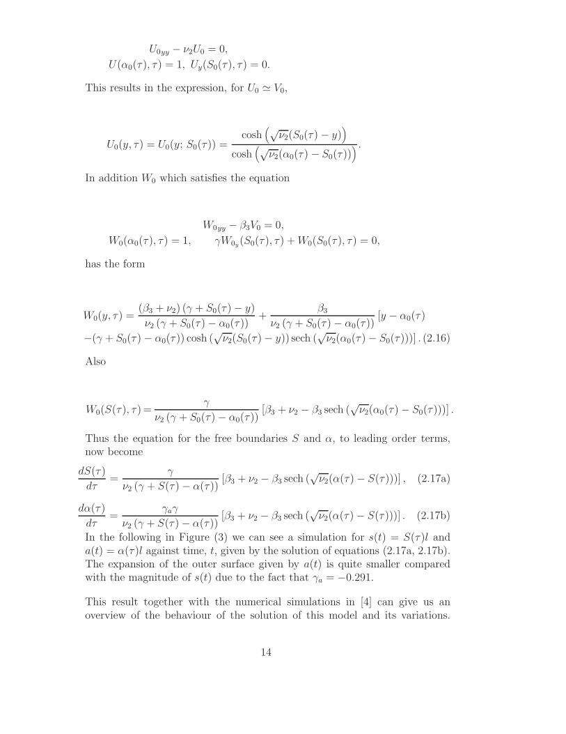
Thus the equation for the free boundaries S and α, to leading order terms,now become

dS(τ)

dτ=

γ

ν2 (γ + S(τ) − α(τ))[β3 + ν2 − β3 sech (

√ν2(α(τ) − S(τ)))] , (2.17a)

dα(τ)

dτ=

γaγ

ν2 (γ + S(τ) − α(τ))[β3 + ν2 − β3 sech (

√ν2(α(τ) − S(τ)))] . (2.17b)

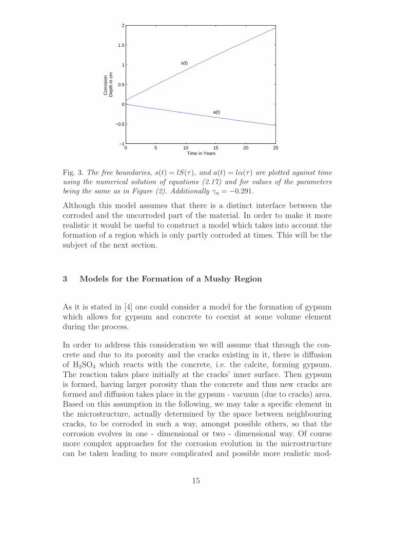
In the following in Figure (3) we can see a simulation for s(t) = S(τ)l anda(t) = α(τ)l against time, t, given by the solution of equations (2.17a, 2.17b).The expansion of the outer surface given by a(t) is quite smaller comparedwith the magnitude of s(t) due to the fact that γa = −0.291.

This result together with the numerical simulations in [4] can give us anoverview of the behaviour of the solution of this model and its variations.

14

0 5 10 15 20 25−1

−0.5

0

0.5

1

1.5

2

Time in Years

Cor

rosi

on

Dep

th in

cm

s(t)

a(t)

Fig. 3. The free boundaries, s(t) = lS(τ), and a(t) = lα(τ) are plotted against timeusing the numerical solution of equations (2.17) and for values of the parametersbeing the same as in Figure (2). Additionally γa = −0.291.

Although this model assumes that there is a distinct interface between thecorroded and the uncorroded part of the material. In order to make it morerealistic it would be useful to construct a model which takes into account theformation of a region which is only partly corroded at times. This will be thesubject of the next section.

3 Models for the Formation of a Mushy Region

As it is stated in [4] one could consider a model for the formation of gypsumwhich allows for gypsum and concrete to coexist at some volume elementduring the process.

In order to address this consideration we will assume that through the con-crete and due to its porosity and the cracks existing in it, there is diffusionof H2SO4 which reacts with the concrete, i.e. the calcite, forming gypsum.The reaction takes place initially at the cracks’ inner surface. Then gypsumis formed, having larger porosity than the concrete and thus new cracks areformed and diffusion takes place in the gypsum - vacuum (due to cracks) area.Based on this assumption in the following, we may take a specific element inthe microstructure, actually determined by the space between neighbouringcracks, to be corroded in such a way, amongst possible others, so that thecorrosion evolves in one - dimensional or two - dimensional way. Of coursemore complex approaches for the corrosion evolution in the microstructurecan be taken leading to more complicated and possible more realistic mod-

15

els. Although the basic qualitative characteristics of the models of these kindshould be apparent by the microstructure considerations presented here.

Note also that due to the difference in the densities of the calcite and thegypsum we may have an expansion of overall volume of the system. To keepthings simple we will assume in the following of this work that this volumeexpansion is negligible and will not be further considered.

3.1 A One - Dimensional Model

Initially we will adopt a one - dimensional consideration regarding the geome-try of the porous medium in the microstructure. We assume that it consists ofmaterial, CaCO3, containing long-narrow cylindrical cracks, equispaced, andparallel between them. This assumption simplifies significantly the analysisthat follows and we have to note that typical crack formations in concrete,(see e.g. [6], [7], [11]) indicate that the above assumption can be taken as aplausible first step to construct a fairly realistic model. Moreover note that wemay consider a large in number set of pores and an additional one intersect-ing each one of them, so that to allow diffusion of liquid in the system. Nearthe cross sections of the pores we will have a certain behaviour during theprocess of corrosion which differs from the behaviour observed away from theintersections between the parallel pores. For simplicity reasons the behaviournear the intersections will not be taken into account in the models derivedin the following. More specifically we will assume that the evolution of corro-sion near the cross section of the pores does not effect significantly the overallprocess and in this work we will study only the corrosion process of poreswhich are parallel to each other. This consideration also accounts for the two- dimensional model derived in the next section.

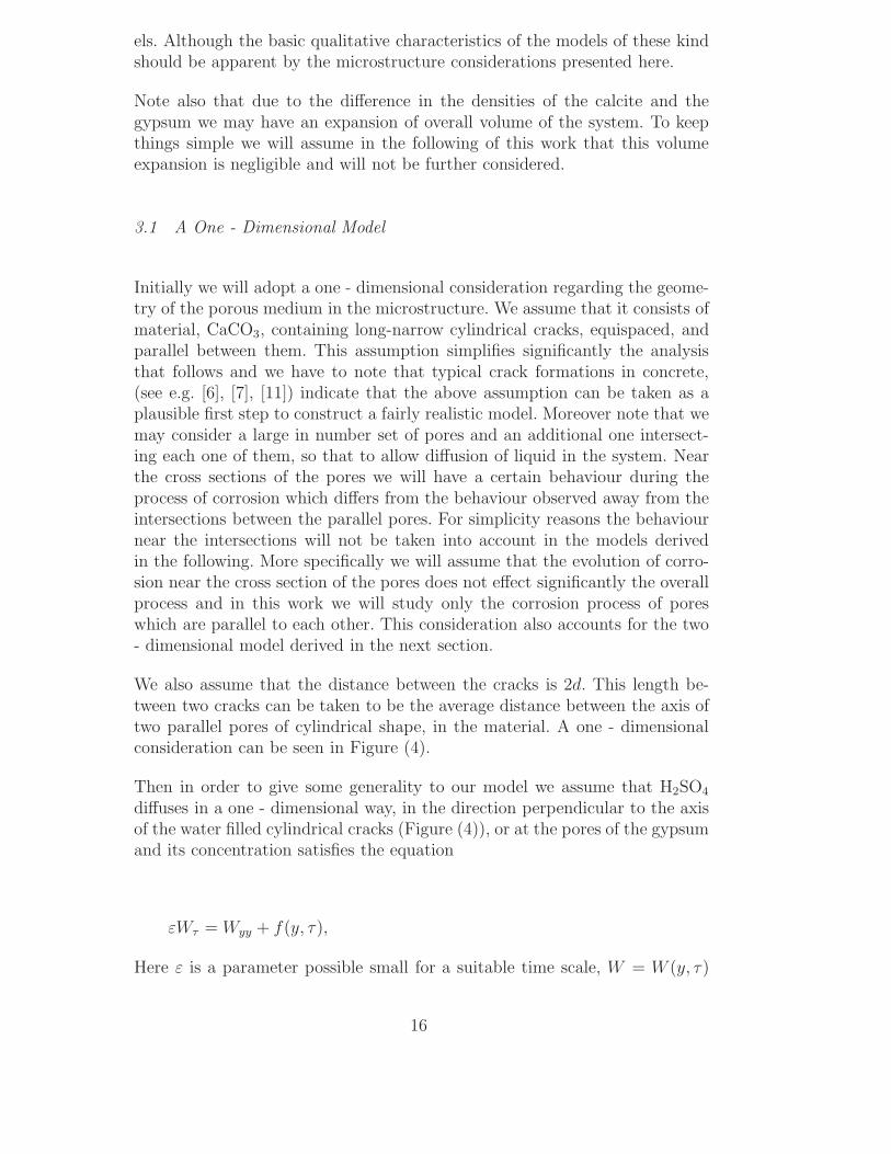
We also assume that the distance between the cracks is 2d. This length be-tween two cracks can be taken to be the average distance between the axis oftwo parallel pores of cylindrical shape, in the material. A one - dimensionalconsideration can be seen in Figure (4).

Then in order to give some generality to our model we assume that H2SO4

diffuses in a one - dimensional way, in the direction perpendicular to the axisof the water filled cylindrical cracks (Figure (4)), or at the pores of the gypsumand its concentration satisfies the equation

εWτ = Wyy + f(y, τ),

Here ε is a parameter possible small for a suitable time scale, W = W (y, τ)

16

again is the dimensionless concentration of H2SO4, y the dimensionless spacevariable (y = x

lfor x the dimensional space variable and l being a typical

macroscopic length), τ the dimensionless time and f is some source term. Inthe pipe corrosion example f is β3V (y, τ) and ε corresponds to ε3.

Concrete ConcreteVacant

Vacant

Vacant

A

B R−Ro R−Ro

Vacant

Concrete

2Ro

S Sl r Sl

z=2z=0

R−Ro 2Ro

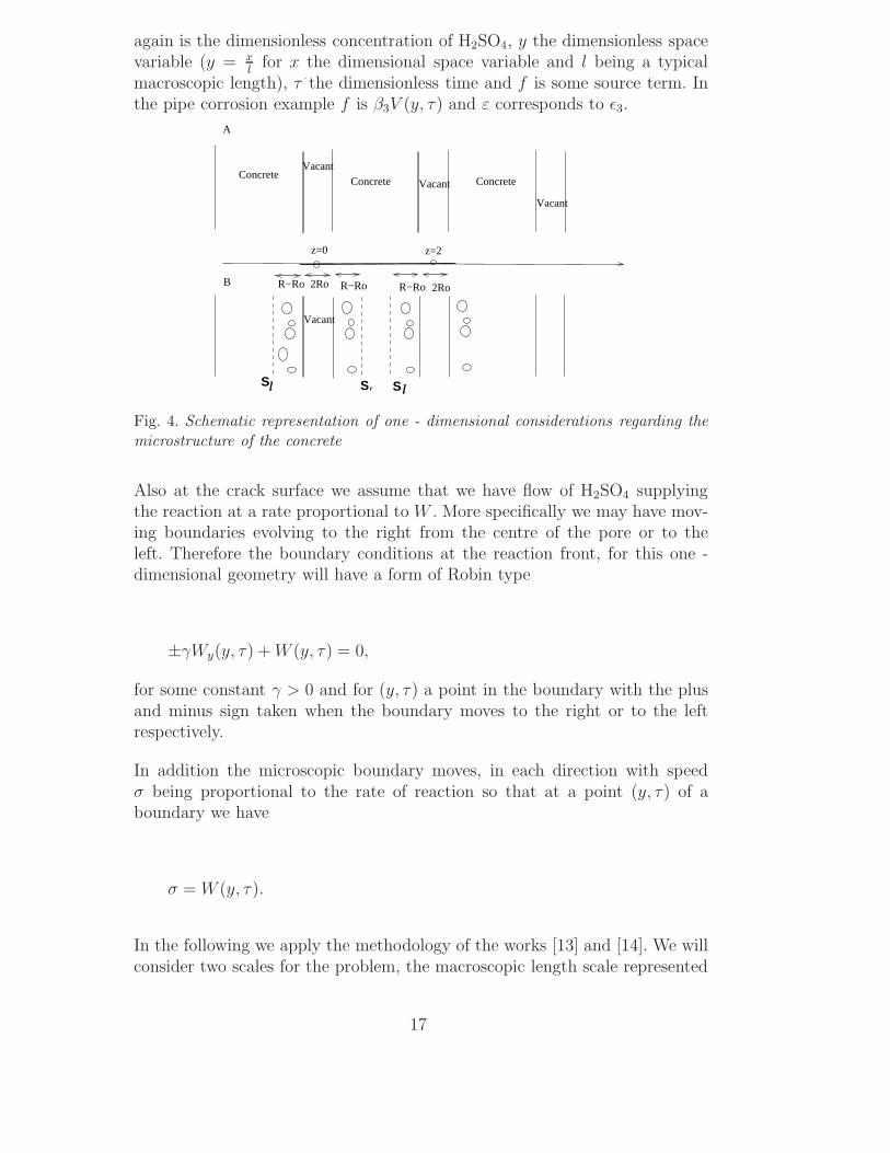
Fig. 4. Schematic representation of one - dimensional considerations regarding themicrostructure of the concrete

Also at the crack surface we assume that we have flow of H2SO4 supplyingthe reaction at a rate proportional to W . More specifically we may have mov-ing boundaries evolving to the right from the centre of the pore or to theleft. Therefore the boundary conditions at the reaction front, for this one -dimensional geometry will have a form of Robin type

±γWy(y, τ) + W (y, τ) = 0,

for some constant γ > 0 and for (y, τ) a point in the boundary with the plusand minus sign taken when the boundary moves to the right or to the leftrespectively.

In addition the microscopic boundary moves, in each direction with speedσ being proportional to the rate of reaction so that at a point (y, τ) of aboundary we have

σ = W (y, τ).

In the following we apply the methodology of the works [13] and [14]. We willconsider two scales for the problem, the macroscopic length scale represented

17

by the variable y and a microscopic length scale represented by the variable z.As it is already mentioned l is a typical macroscopic length, say the width ofa concrete slab or the thickness of a wall etc., whose corrosion is being studiedand in addition we consider 2d to be the distance between the centre of twoparallel pores of the material. Note that d l. As a next step we take

W = W (y, z, τ),

where x = ly and x = dz with δ = dl 1. In addition we scale the dimensional

position of the boundary, say s, with d, i.e. S = sd

where S is the dimensionlessposition of the moving boundary and we make an appropriate choice of thetime scale so that to balance the terms in the Stefan condition, e.g. in the pipecorrosion example we take now t0 = Ccd

Kcλ3. Moreover motivated by the form of

the corresponding constant in equation (2.8c) we have γ = DH

Kcl= dDH

Kcl2ld

= γm1δ,

for γm = dDH

Kcl2. Thus in the following we will set γ = γm

1δ

and we will assumethat γm = O(1).

The multiple scales approach gives instead for the spatial derivative ∂W∂y

at a

point (y, z, τ), the expression

∂W

∂y+

1

δ

∂W

∂z,

and the equation for W = W (y, z, τ) will be

εWτ = Wyy +1

δ2Wyy + f.

Also at the moving boundaries where z = S, the one moving to the left S = Sl

and the one moving to the right S = Sr, we have the boundary condition ofRobin type which now becomes

±γm

1

δ

(

Wy(y, S, τ) +1

δ

∂W

∂z(y, S, τ)

)

+ W (y, S, τ) = 0.

Finally the Stefan condition, at the points (y, S, τ), S = Sr, Sl, and for achoice of the appropriate time scale, takes the form

±dS

dτ= W (y, S, τ),

18

where the plus sign accounts for S = Sr, increasing and the minus for S = Sl

decreasing. Also the width of the pores initially is equal to R0 (see Figure(4A)). As it is already stated the corrosion process evolves and two free bound-aries appear. We set the centre of one pore to be taken at z = 0 while thecentre of the parallel pore (with the same initial width) can be set at z = 2and we take one front having distance R from z = 0, Sr = R ≥ R0 andmoving to the right and the other, Sl, moving to the left and due to sym-metry, having similarly, distance R from the point z = 2, i.e. Sl = 2 − R(see Figure (4B)). This means that the dimensionless width of the remain-ing concrete is 2 − 2R, while the dimensionless width of the vacant - gypsumsystem is 2R. Note that for S = Sr by the Stefan condition and the Robincondition applied we take dSr

dτ= −1

δγm(Wy + 1

δWz) while for S = Sl similarly

−dSl

dτ= W = 1

δγm(Wy + 1

δWz) and in both cases δ dS

dτ= −γm(Wy + 1

δWz).

In addition due to the fact that we have infinite amount of pores parallel toeach other which are undistinguished we may consider periodic conditions atthe ends of an interval determined by the centres of two parallel pores, z = 0and z = 2 and which is representative of the structure of the material. Hencewe set periodic conditions at the boundary of the interval [0, 2], i.e.

[W ]20 = 0, [Wz + δWy]20 = 0.

Therefore, by assuming that the source term can be written in the form

f(y, τ) = f0(y, τ) + δf1(y, τ) + . . . ,

and that W ∼ W0 + δW1 + . . ., the basic field equation, at the points (y, z, τ)with z ∈ Ωg := [0, R] ∪ [2 − R, 2], takes the form

εW0τ + εδW1τ + εδ2W2τ + . . .=1

δ2W0zz +

2

δW0zy + W0yy + f0

+1

δW1zz + 2W1zy + δW1yy + δf1

+W2zz + 2δW2zy + δ2W2yy + δ2f2

+δW3zz + 2δ2W3zy + . . . .

At the free boundaries formed during corrosion S = Sr, Sl, we have for S ∼S0+δS1+. . ., and W (y, S0+δ S1+. . . , τ) ∼ W (y, S0, τ)+δ S1Wz(y, S0, τ)+. . .,that

19

±γm

(

1

δ2W0z +

1

δW0y +

1

δW1z + W1y + W2z +

1

δS1W0zz + S1W0yz + S1W1zz + . . .

)

+W0 + δW1 + δS1W0z + . . .=0,

at the points (y, S0, τ).

In addition the free boundary condition at the same points will become

dS0

dτ+ δ

dS1

dτ+ . . . = −γm

(

1

δ2W0z +

1

δW0y +

1

δW1z + W1y + W2z + δW2y + δW3z

+1

δS1W0zz + S1W0yz + S1W1zz + . . .

)

.

Similarly the periodic conditions at z = 0, 2, have the form

[

1

δ2W0 +

1

δW1 + W2 + . . .

]z=2

z=0= 0,

and

[

1

δ2W0z +

1

δW0y +

1

δW1z + W1y + W2z + . . .

]z=2

z=0= 0.

Equating O( 1δ2 ) terms we obtain

W0zz = 0,

at the points (y, z, τ) with z ∈ Ωg, while by the periodic conditions at z = 0, 2we have

[W0z]z=2z=0 = 0, [W0]

z=2z=0 = 0.

Also at z = S = Sr, Sl ∼ S0 we have

W0z = 0.

20

The above equations implies that W0z(y, z, τ) = 0 and consequently thatW0 = W0(y, τ).

For the O(1δ) terms similarly, given that W0 = W0(y, τ), we have

W1zz = 0,

at the points (y, z, τ) with z ∈ Ωg, with the relevant periodic conditions at z =

0, 2 being[

W0y + W1z

]z=2

z=0= 0 and [W1]

z=2z=0 = 0. Also at z = S = Sr, Sl ∼ S0

we have W0y + W1z = 0, to leading order terms. Therefore again as for W0 wededuce that W1z = 0 or that W1 = W1(y, τ).

Continuing for O(1) terms, and for z ∈ Ωg, we have

εW0τ = W0yy + W2zz + f0, (3.1)

with the conditions

[W2]z=2z=0 = 0,

[

W1y + W2z

]z=2

z=0= 0,

at the points (y, 0, τ), (y, 2, τ), and

±γm(W1y + W2z) + W0 = 0,

at z = S = Sr, Sl ∼ S0. In addition the equation for S will give

dS0(τ)

dτ= −γm

(

W1y + W2z

)

at z = S = Sr, Sl ∼ S0 to leading order terms.

Averaging equation (3.1) over z will result, due to the periodic conditionsapplied at the ends of the interval [0, 2], in the equation,

∫ Sr

0+∫ 2

Sl

[

εW0τ − W0yy

]

dz =∫ Sr

0+∫ 2

Sl

f0(y, τ)dz

+W2z|z=2 − W2z|z=Sl+ W2z|z=Sr

− W2z|z=0.

21

Due to the periodic conditions [W2]z=2z=0 = 0 and

[

W1y + W2z

]z=2

z=0= 0, the

condition for the free boundary

[W2z]z=Sr= − 1

γm

dSr(τ)

dτ−[

W1y

]

z=Sr

,

[W2z]z=Sl= − 1

γm

dSl(τ)

dτ−[

W1y

]

z=Sl

,

and the fact that W1 = W1(y, τ) which implies that W1 does not vary signifi-cantly over z ∈ [0, 2] giving [W1y]

z=2z=0 = 0, [W1y]

z=Sl

z=Sr= 0, we obtain finally, for

φg being the constant gypsum porosity and for Sl = 2 − R, Sr = R, that

2Rφg

[

εW0τ − W0yy − f0(y, τ)]

=1

γm

(

−dSr(τ)

dτ+

dSl(τ)

dτ

)

=1

γm

(

−∂R

∂τ+

∂(2 − R)

∂τ

)

= − 2

γm

∂R

∂τ.

By denoting with W the dominant term W0 we have the macroscopic equation

εWτ = Wyy + f0(y, τ) − 1

γmφgR

∂R

∂τ, (3.2)

with

∂R

∂τ=

0, R = R0 and τ < τ1(y), or R = 1 and τ > τ2(y),

W (y, τ), R0 < R < 1,(3.3)

and R(y, 0) = R0. The time τ1(y) denotes the time when W (y, τ) becomespositive for the first time at the point y and τ2(y) denotes the time when Rreaches one at the same point. For W (y, τ) > 0, R increases starting from R0

till it reaches the value R = 1. Note also that R should depend only on thetime τ and the macroscopic position y, R = R(y, τ) as it is also emerge fromequation (3.3).

This equation applies for the actual concentration W of a substance containedin the water inside the pores of the material. In order to measure the effective

22

concentration we take this to be W = φW , where φ = φ(y, τ) is the porosityof the material corresponding to the interval [0, 2] i.e. the ratio of vacant overthe total volume of the material in [0, 2]. When the whole of the material inthe interval [0, 2] is uncorroded we have φ = φc and the initial radius of thepore is fixed so that R0 = φc, while when it is fully corroded φ = φg. Hence wehave φc < φ < φg, for φ depending directly from R = R(y, τ) via the relation

φ(y, τ) = φ(R(y, τ)) = (R(y,τ)+φb)φa

, where φa = 1−φc

φg−φcand φb = φc(1−φg)

φg−φcare

appropriate constants giving φ(R0) = φc and φ(1) = φg.

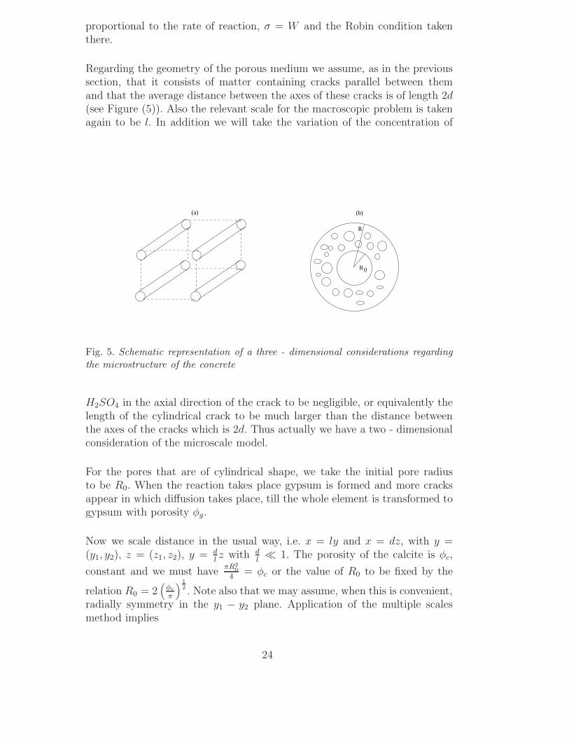
Therefore the system of equations (3.2) and (3.3) with appropriate boundaryand initial conditions form a phase field model for concrete corrosion. Up tothis point we have considered the gypsum evolving in a one - dimensionaldirection and actually taking as an element characterizing the microstructureof the material the interval [0, 2d]. We can continue with a more realisticapproach by considering instead such a microscopic element to be a square,with side 2d and having at its four corners pores of radius R0 centered at thevertexes of this square (see Figure (5)).

3.2 A Two - Dimensional Model

Again we consider the equation

εWτ = ∆W + f(y, τ),

with f being the source term and y = (y1, y2). The diffusion takes place nowin two spatial dimensions. In addition the boundary condition at the interfaceΓ of the corroded - uncorroded material will be

γm

1

δ

∂W

∂n+ W = 0, y ∈ Γ,

where n is the outward normal vector at a point of the moving boundary Γ,while the motion of the boundary is given by the standard Stefan condition

−γm

∂W

∂n= σ, y ∈ Γ

where σ is the speed of the moving boundary. The latter comes from the fact,as in the one - dimensional case, that the speed of the moving boundary Γ is

23

proportional to the rate of reaction, σ = W and the Robin condition takenthere.

Regarding the geometry of the porous medium we assume, as in the previoussection, that it consists of matter containing cracks parallel between themand that the average distance between the axes of these cracks is of length 2d(see Figure (5)). Also the relevant scale for the macroscopic problem is takenagain to be l. In addition we will take the variation of the concentration of

(a)

R0

R

(b)

Fig. 5. Schematic representation of a three - dimensional considerations regardingthe microstructure of the concrete

H2SO4 in the axial direction of the crack to be negligible, or equivalently thelength of the cylindrical crack to be much larger than the distance betweenthe axes of the cracks which is 2d. Thus actually we have a two - dimensionalconsideration of the microscale model.

For the pores that are of cylindrical shape, we take the initial pore radiusto be R0. When the reaction takes place gypsum is formed and more cracksappear in which diffusion takes place, till the whole element is transformed togypsum with porosity φg.

Now we scale distance in the usual way, i.e. x = ly and x = dz, with y =(y1, y2), z = (z1, z2), y = d

lz with d

l 1. The porosity of the calcite is φc,

constant and we must haveπR2

0

4= φc or the value of R0 to be fixed by the

relation R0 = 2(

φc

π

) 1

2 . Note also that we may assume, when this is convenient,radially symmetry in the y1 − y2 plane. Application of the multiple scalesmethod implies

24

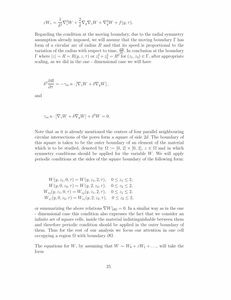
εWτ =1

δ2∇2

zW +2

δ∇y∇zW + ∇2

yW + f(y, τ).

Regarding the condition at the moving boundary, due to the radial symmetryassumption already imposed, we will assume that the moving boundary Γ hasform of a circular arc of radius R and that its speed is proportional to thevariation of the radius with respect to time, ∂R

∂τ. In conclusion at the boundary

Γ where |z| = R = R(y, z, τ) or z21 +z2

2 = R2 for (z1, z2) ∈ Γ, after appropriatescaling, as we did in the one - dimensional case we will have

δ2∂R

∂τ= −γm n · [∇zW + δ∇yW ] ,

and

γm n · [∇zW + δ∇yW ] + δ2W = 0.

Note that as it is already mentioned the centres of four parallel neighbouringcircular intersections of the pores form a square of side 2d. The boundary ofthis square is taken to be the outer boundary of an element of the materialwhich is to be studied, denoted by Ω := [0, 2] × [0, 2], z ∈ Ω and in whichsymmetry conditions should be applied for the variable W . We will applyperiodic conditions at the sides of the square boundary of the following form:

W (y, z1, 0, τ) = W (y, z1, 2, τ), 0 ≤ z1 ≤ 2,

W (y, 0, z2, τ) = W (y, 2, z2, τ), 0 ≤ z2 ≤ 2,

Wz2(y, z1, 0, τ) = Wz2

(y, z1, 2, τ), 0 ≤ z1 ≤ 2,

Wz1(y, 0, z2, τ) = Wz1

(y, 2, z2, τ), 0 ≤ z2 ≤ 2,

or summarizing the above relations ∇W |∂Ω = 0. In a similar way as in the one- dimensional case this condition also expresses the fact that we consider aninfinite set of square cells, inside the material indistinguishable between themand therefore periodic condition should be applied in the outer boundary ofthem. Thus for the rest of our analysis we focus our attention in one celloccupying a region Ω with boundary ∂Ω.

The equations for W , by assuming that W ∼ W0 + εW1 + . . ., will take theform

25

εW0τ + δεW1τ + δ2εW2τ + . . .=1

δ2∇2

zW0 +2

δ∇z∇yW0 + ∇2

yW0 + f0

+1

δ∇2

zW1 + 2∇z∇yW1 + δ∇2yW1 + δf1

+∇2zW2 + 2δ∇z∇yW2 + δ2∇2

yW2 + δ2f2

+δ∇2zW3 + 2δ2∇z∇yW3 + . . . .

Also at the points (y, z, τ) with z = (z1, z2) ∈ Γ, we have that

∂R

∂τ= −γm n ·

[

1

δ2∇zW0 +

1

δ∇yW0 +

1

δ∇zW1 + ∇yW1 + ∇zW2 + . . .

]

,

W0 + . . . + γm n ·[

1

δ2∇zW0 +

1

δ∇yW0 +

1

δ∇zW1 + ∇yW1 + ∇zW2 + . . .

]

= 0.

Then for order O( 1δ2 ) terms we have ∇2

zW0 = 0. By the conditions at themoving boundary Γ, i.e. at z = R we get n · ∇zW0 = 0. In addition at the cellboundary, ∂Ω we have again n · ∇zW0 = 0. By these equations and a directapplication of the maximum principle we deduce that W0 = W0(y, τ).

For order O(1δ) terms we have 2∇z∇yW0+∇2

zW1 = 0, or ∇2zW1 = 0 due to the

fact that W0 = W0(y, τ). In addition at z = R we have n · [∇yW0 + ∇zW1] = 0while at the cell boundary, ∂Ω we have similarly n·[∇yW0 + ∇zW1] = 0. As forthe O( 1

δ2 ) terms by using the same arguments and the fact that n · ∇yW0 = 0over the boundary because W0 does not vary significantly in the z−scale, wededuce that W1 = W1(y, τ).

For O(1) terms, given that ∇zW1 = 0, we have

εW0τ = ∇2yW0 + ∇2

zW2 + f0(y, τ),

while at z = R,

∂R

∂τ= −γm n · [∇yW1 + ∇zW2] .

As for the one - dimensional case we may proceed by averaging the field equa-tion over the whole domain occupied by the gypsum or vacants, say Ωg. Due

26

to the fact that periodic conditions are applied to each of the indistinguishablecells averaging of the equation for W0 will result in the following equation:

∫

Ωg

[

εW0τ −∇2yW0 − f0(y, τ)

]

dz =∫

Ωg

∇2zW2dz =

∫

Γ∪Γe

n · ∇zW2dz,

for Γe = ∂Ω⋂

∂Ωg, or

φgA(R)[

εW0τ −∇2yW0 − f0(y, τ)

]

=∫

Γn · ∇zW2dz +

∫

Γe

n · ∇zW2dz,

where A(R) is the area of the cell occupied by the gypsum. Note that the

z =11

2Rd

R

1−Rd

Rd

1−Rd

Rd

z =11

R

z =12

(0,0)

z =0

z =0z =2

z =2

1 1

2

2

(B)z =1

z =11

2

R

z =1

(A)(0,0)

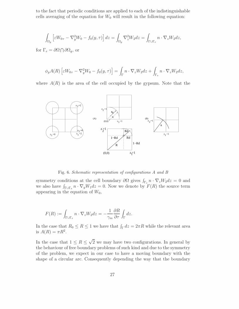
Fig. 6. Schematic representation of configurations A and B

symmetry conditions at the cell boundary ∂Ω gives∫

Γen · ∇zW2dz = 0 and

we also have∫

Γ∪Γen · ∇yW1dz = 0. Now we denote by F (R) the source term

appearing in the equation of W0,

F (R) :=∫

Γ∪Γe

n · ∇zW2dz = − 1

γm

∂R

∂τ

∫

Γdz.

In the case that R0 ≤ R ≤ 1 we have that∫

Γ dz = 2πR while the relevant areais A(R) = πR2.

In the case that 1 ≤ R ≤√

2 we may have two configurations. In general bythe behaviour of free boundary problems of such kind and due to the symmetryof the problem, we expect in our case to have a moving boundary with theshape of a circular arc. Consequently depending the way that the boundary

27

intersects with the lines z1 = 1, 0 ≤ z2 ≤ 2 or z2 = 1, 0 ≤ z1 ≤ 2 insidethe square element we may have two different configurations (see Figure (6)).We may assume that after the time the radius R exceeds one, the circulararc is tangent to these lines, or that it intersects them with its tangent at theintersection points, forming some angle with it (see also [13]).

Case A The boundary is a circle arc tangent to the lines z1 = 1 andz2 = 1. In this case the area of the gypsum in one of the quarters of the cell,Ω = [0, 2]× [0, 2], will be the sum of three rectangles and a circular segment ofradius Rd, where Rd is the radius of the circle which its circular arc is tangentto the lines z1 = 1, 0 ≤ z2 ≤ 2 and z2 = 1, 0 ≤ z1 ≤ 2. Thus the area occupied

by the gypsum in this quarter will be 2Rd(1− Rd) + (1− Rd)2 +

πR2d

4and the

area of the gypsum in the whole cell will be A(R) = 4(

1 − R2d(1 − π

4))

(see

Figure 6A). Also if R, measures the distance from the point of intersection ofthe circular arc and the line z2 = z1 to the point (z1, z2) = (0, 0) we have that

(R − Rd) +√

2Rd =√

2 or that Rd = R−√

21−

√2. In addition the overall length of

the arcs consisting the boundary Γ, is L(R) = 2πRd.

In this case the field equation, by denoting with W the dominant term W0,becomes

εWτ = ∇2yW + f0(y, τ) + F (R), (3.4)

with

F (R) =

− 2γmφg

1R

∂R∂τ

, R0 ≤ R ≤ 1,

− πRd

2γmφg[1−R2d(1−π

4)]

∂R∂τ

, 1 < R ≤√

2,(3.5)

In addition to leading order terms, by the Robbin condition at the movingboundary Γ, γm n · ∇W + W = 0 we obtain the equation for macroscopicvariable R which is

∂R

∂τ= W (y, τ). (3.6)

Case B The boundary is a circle that has radius R and at all times in-tersects the lines z1 = 1 and z2 = 1 at some angle φ. In this case L(R) =

28

2R[

π − 4 cos−1(

1R

)]

and A(R) = 4[√

R2 − 1 + R2

2

(

π2− 2 cos−1

(

1R

))]

. Then

the field equation is again given by equation (3.4) and (3.6) but with

F (R) =

− 2γmφg

1R

∂R∂τ

, R0 ≤ R ≤ 1,

− R[π−4 cos−1( 1

R)]

2γmφg

[√R2−1+ R2

4 (π−4 cos−1( 1

R))]

∂R∂τ

, 1 < R ≤√

2.(3.7)

4 Numerical Solution

In order to obtain a numerical solution of the various phase field models de-rived in Section (3) we will use a finite element method, regarding space dis-cretization, combined with the two step Crank- Nicholson method, indicatingthat the scheme is unconditionally stable.

Initially we will solve numerically the model given by equations (3.2) and(3.3). Note that as it is already mentioned these equations account for theactual concentration W of SO2−

4 while the effective concentration W is givenby W = φW , for φ being the porosity of the material, φ = φ(y, τ). In addition,

given that R(y, 0) = R0 = φc we have that φ = φc + (R − φc)(φg−φc)

1−φcor that

R =(

1−φc

φg−φc

)

φ − φc1−φc

φg−φcand ∂R

∂τ=(

1−φc

φg−φc

)

∂φ

∂τ. We will consider a uniform

cement slab with y ∈ [0, 1] (this may come after appropriate scaling) andwe will also take no flux, Neumann condition at y = 1 corresponding to anassumption of symmetry. The latter may be the case when we examine a wallof dimensionless length 2 exposed in H2SO4 from both sides. Alternativelythis no flux condition may result in the case where the right part of the wall isisolated. At y = 0 we assume that the effective concentration is equal to one.

Then the system of equations to be solved takes the form of equations (3.2)and (3.3) together with the following boundary and initial conditions

φ(0, τ)W (0, τ) = 1,∂

∂y(φ(1, τ)W (1, τ)) = 0, (4.1)

W (y, 0) = 0, R(y, 0) = 0. (4.2)

We discretize the system of equations in the following way. We consider a gridof the domain [0, 1]×[0, T ], where T is the final time of a potential simulation.Regarding the interval [0, 1] we take M + 1 points yj = j · δy for δy beingthe spatial step for j = 0, 1, 2, · · ·M . In addition in the interval [0, T ] we take

29

N time steps of size δτ , where N = [T/δτ ] and with the points of the timediscretization being τi = iδτ , i = 1, 2, . . .N .

Let Φj , j = 0, . . . , M denote the standard linear B - splines on the interval[0, 1], defined with respect to the partition considered.

Φj =

y−yj−1

δy, yj−1 ≤ y ≤ yj,

yj+1−y

δy, yj ≤ y ≤ yj+1,

0, elsewhere in [0, 1],

(4.3)

for j = 0, 1, 2, . . . , M . We then set W (y, τ) =∑M

j=0 awj(τ)Φj(y), and R(y, τ) =

∑Mj=0 aRj

(τ)Φj(y), τ ≥ 0, 0 ≤ y ≤ 1.

Substituting these expressions for W and R into the relevant equations andapplying the standard Galerkin method, i.e. multiplying with Φi, for i =1, 2, . . . , M and integrating over [0, 1] we obtain a system of equations for theaw’s and the aR’s.

εM∑

j=0

awj(τ) < Φj(y) Φi(y) >=−

M∑

j=0

awj(τ) < Φ′

j(y) Φ′i(y) >

+ < F

M∑

j=0

aRj(τ)Φj(y)

Φi(y) >, (4.4)

aRj(τ) = awj

(τ), (4.5)

where < f, g >:=∫ 10 f(y)g(y)dy and i = 1, 2, . . . , M . Setting aw = [aw1

, aw2, . . . , awM

]T

and aR = [aR1, aR2

, . . . , aRM]T the system of equations for the aw’s and the

aR’s take the form

Aaw(τ) =−Baw(τ) + b(τ),

aR(τ) = aw(τ),

where, taking also into account the boundary conditions, (4.1), and (4.2) thematrices A, B and b have the form

30

A = εδy

23

16 0 . . . 0

16

23

16 . . . 0

0 0. . .

. . . 0

0 0 . . . 16

13

, B =1

δy

2 −1 0 . . . 0

−1 2 −1 . . . 0

0 0. . .

. . . 0

0 0 . . . −1φy(1)φ(1) + 1

, b(t) =

1φ(0)+ < F (R),Φ1 >

< F (R),Φ2 >

...

< F (R),ΦM >

We then apply the three time step approximation by taking aw(τn) ' an+1w −an−1

w

2δτ.

The relevant equation then becomes

A

(

an+1w − an−1

w

2δτ

)

= −B

(

an+1w + an−1

w

2

)

+ bn,

where bn = b(tn).

After some manipulation we obtain the equations

an+1w = (A + δτB)−1

[

(A − δτB)an−1w + 2δτ bn

]

, (4.6a)

an+1R = an−1

R + 2δτanw. (4.6b)

Note that for the second time step we have in place of equations (4.6).

a2w = (A + δτB)−1

[

(A − δτB)a1w + δτ b1

]

, (4.7a)

a2R = a1

R + δτa1w, (4.7b)

for a1w and a1

R being determined by the initial conditions.

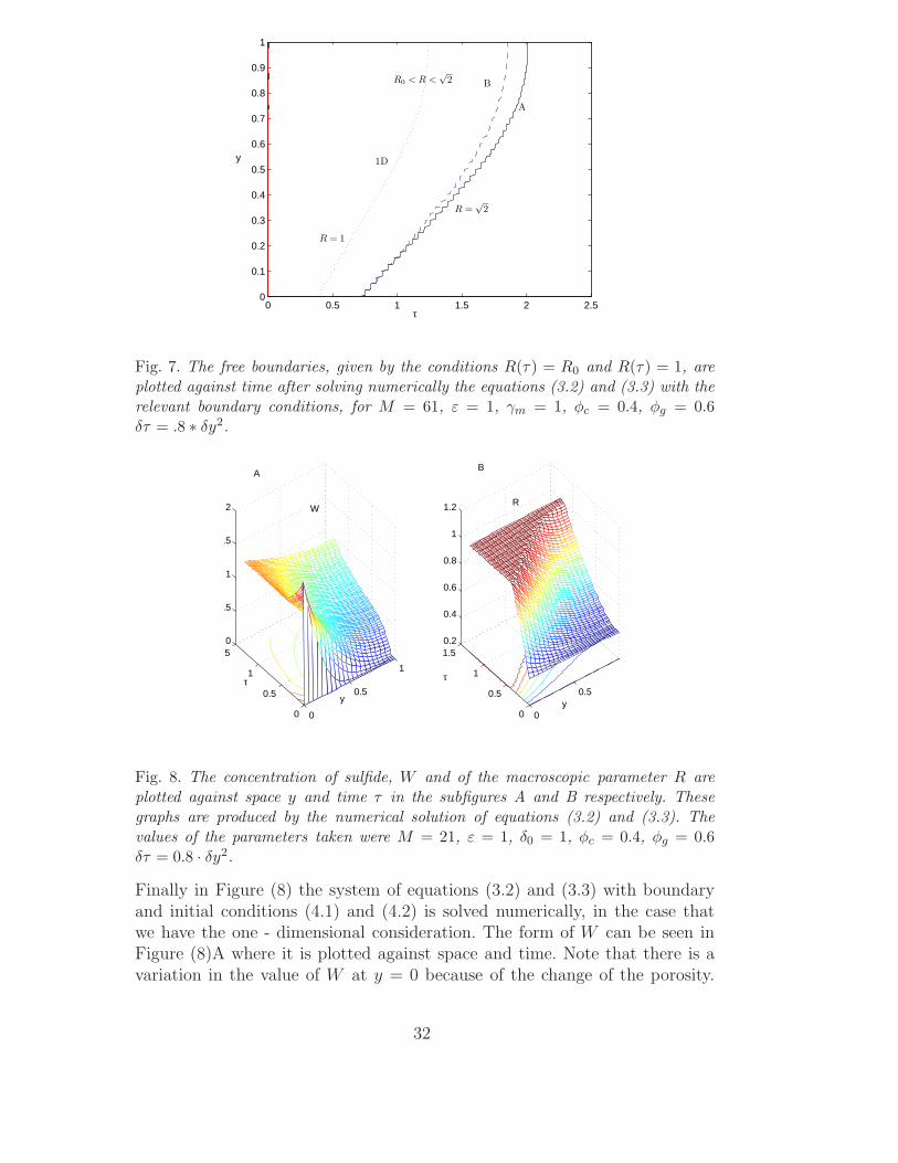
In Figure (7) the system of equations (3.2) and (3.3) with the boundary andinitial conditions (4.1) and (4.2), is solved numerically and the free boundariesgiven by the conditions R(y, τ) = R0 and R(y, τ) = 1 (dotted line), are plottedagainst time. Also in the same Figure (7) the system of equations (3.2) and(3.3) with the same boundary conditions is solved numerically, in the case thatconfiguration A (solid line) and B (dashed line) are considered, i.e. for sourceterms given by equations (3.5) and (3.6). For these cases the free boundariesgiven by the conditions R(y, τ) = R0 and R(y, τ) =

√2, are plotted against

time. The lower boundaries coincide while the upper boundaries are distinctiveindicating that in the case of configuration A the transition into gypsum takesplace slower at the inner part of the material. Note also that in all of theabove simulations the lower boundary is a line parallel to the spatial axis(some small variations are not visible in the Figure). This indicates that almostimmediately, at τ = 0, the whole of the material enters the mushy region andfor all y ∈ [0, 1] the material is partly corroded with R(y, τ) exceeding R0, forτ ≥ 0.

31

0 0.5 1 1.5 2 2.50

0.1

0.2

0.3

0.4

0.5

0.6

0.7

0.8

0.9

1

R0 < R <√

2

R =√

2

R = 1

1D

B

A

y

τ

Fig. 7. The free boundaries, given by the conditions R(τ) = R0 and R(τ) = 1, areplotted against time after solving numerically the equations (3.2) and (3.3) with therelevant boundary conditions, for M = 61, ε = 1, γm = 1, φc = 0.4, φg = 0.6δτ = .8 ∗ δy2.

0

0.5

0

0.5

1

1.50.2

0.4

0.6

0.8

1

1.2

0

0.5

1

0

0.5

1

1.50

0.5

1

1.5

2 WR

y y

τ τ

AB

Fig. 8. The concentration of sulfide, W and of the macroscopic parameter R areplotted against space y and time τ in the subfigures A and B respectively. Thesegraphs are produced by the numerical solution of equations (3.2) and (3.3). Thevalues of the parameters taken were M = 21, ε = 1, δ0 = 1, φc = 0.4, φg = 0.6δτ = 0.8 · δy2.

Finally in Figure (8) the system of equations (3.2) and (3.3) with boundaryand initial conditions (4.1) and (4.2) is solved numerically, in the case thatwe have the one - dimensional consideration. The form of W can be seen inFigure (8)A where it is plotted against space and time. Note that there is avariation in the value of W at y = 0 because of the change of the porosity.

32

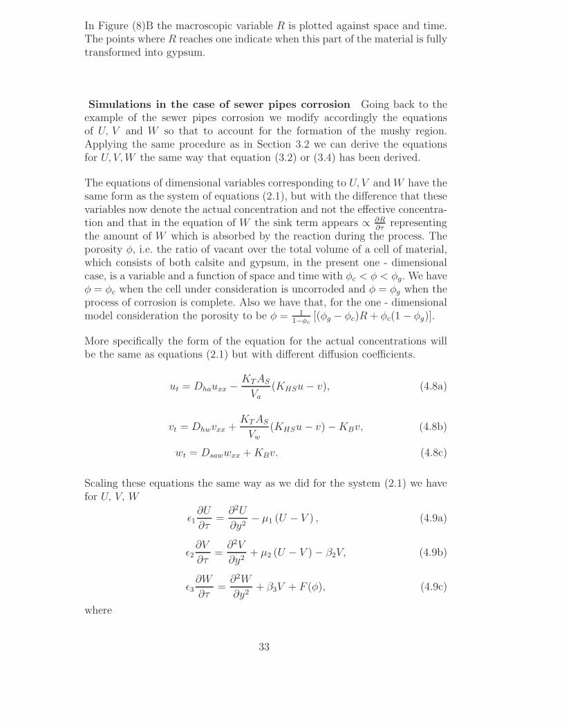
In Figure (8)B the macroscopic variable R is plotted against space and time.The points where R reaches one indicate when this part of the material is fullytransformed into gypsum.

Simulations in the case of sewer pipes corrosion Going back to theexample of the sewer pipes corrosion we modify accordingly the equationsof U, V and W so that to account for the formation of the mushy region.Applying the same procedure as in Section 3.2 we can derive the equationsfor U, V, W the same way that equation (3.2) or (3.4) has been derived.

The equations of dimensional variables corresponding to U, V and W have thesame form as the system of equations (2.1), but with the difference that thesevariables now denote the actual concentration and not the effective concentra-tion and that in the equation of W the sink term appears ∝ ∂R

∂τrepresenting

the amount of W which is absorbed by the reaction during the process. Theporosity φ, i.e. the ratio of vacant over the total volume of a cell of material,which consists of both calsite and gypsum, in the present one - dimensionalcase, is a variable and a function of space and time with φc < φ < φg. We haveφ = φc when the cell under consideration is uncorroded and φ = φg when theprocess of corrosion is complete. Also we have that, for the one - dimensionalmodel consideration the porosity to be φ = 1

1−φc[(φg − φc)R + φc(1 − φg)].

More specifically the form of the equation for the actual concentrations willbe the same as equations (2.1) but with different diffusion coefficients.

ut = Dhauxx −KT AS

Va

(KHSu − v), (4.8a)

vt = Dhwvxx +KT AS

Vw

(KHSu − v) − KBv, (4.8b)

wt = Dsawwxx + KBv. (4.8c)

Scaling these equations the same way as we did for the system (2.1) we havefor U, V, W

ε1∂U

∂τ=

∂2U

∂y2− µ1 (U − V ) , (4.9a)

ε2∂V

∂τ=

∂2V

∂y2+ µ2 (U − V ) − β2V, (4.9b)

ε3∂W

∂τ=

∂2W

∂y2+ β3V + F (φ), (4.9c)

where

33

F (φ) = − φa

γmφg(φaφ − φb)

∂φ

∂τ,

∂φ

∂τ=

1

φa

W (y, τ), (4.10)

for R = φaφ − φb. Also the nondimensional constants now are ε1 = l2

Dhat0,

µ1 = KT Asλ2l2

λ1Dha, ε2 = l2

Dhwt0, µ2 = KT As

l2

Dhw, β2 = KB

l2

Dha, ε3 = l2

Dsawt0,

β3 = kBλ2l2

Dsawλ3for t0 = Ccd

Kcλ3. In addition the boundary conditions have the

following form

φ(0, τ)U(0, τ) = 1, (φ(1, τ)U(1, τ))y = 0, (4.11a)

φ(0, τ)V (0, τ) = 1, (φ(1, τ)V (1, τ))y = 0, (4.11b)

φ(0, τ)W (0, τ) = 1, (φ(1, τ)W (1, τ))y = 0, (4.11c)

Finally at time τ = 0 we have

U(y, 0) = 0, V (y, 0) = 0, W (y, 0) = 0, (4.12a)

φ(y, 0) = φc. (4.12b)

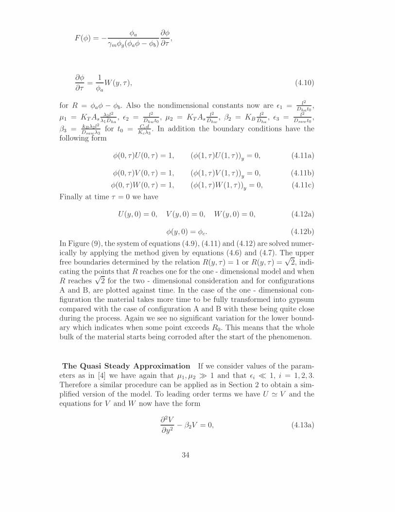
In Figure (9), the system of equations (4.9), (4.11) and (4.12) are solved numer-ically by applying the method given by equations (4.6) and (4.7). The upperfree boundaries determined by the relation R(y, τ) = 1 or R(y, τ) =

√2, indi-

cating the points that R reaches one for the one - dimensional model and whenR reaches

√2 for the two - dimensional consideration and for configurations

A and B, are plotted against time. In the case of the one - dimensional con-figuration the material takes more time to be fully transformed into gypsumcompared with the case of configuration A and B with these being quite closeduring the process. Again we see no significant variation for the lower bound-ary which indicates when some point exceeds R0. This means that the wholebulk of the material starts being corroded after the start of the phenomenon.

The Quasi Steady Approximation If we consider values of the param-eters as in [4] we have again that µ1, µ2 1 and that εi 1, i = 1, 2, 3.Therefore a similar procedure can be applied as in Section 2 to obtain a sim-plified version of the model. To leading order terms we have U ' V and theequations for V and W now have the form

∂2V

∂y2− β2V = 0, (4.13a)

34

−0.2 0 0.2 0.4 0.6 0.8 1 1.2 1.4 1.60

0.1

0.2

0.3

0.4

0.5

0.6

0.7

0.8

0.9

1

τ

A

B

1D

R =√

2

R = R0

y

R = 1

Fig. 9. The free boundaries, given by the conditions R(τ) = R0 and R(τ) =√

2, areplotted against time after solving numerically the equations (4.9), (4.11) and (4.12),but with the source term given by equations (3.3) for the one - dimensional model,(3.6) for configuration A and (3.7) for configuration B, and with the boundary andinitial conditions given by (4.11) and (4.12), for M = 31, ε1 = ε2 = ε3 = 1, γm = 1,β1 = β2 = 1, µ1 = µ2 = 1, φc = 0.4, φg = 0.6, δτ = .8 · δy2.

∂2W

∂y2+ β3V + F (φ) = 0, (4.13b)

combined with equation (4.10), the boundary conditions (4.11b) and (4.11c)and the initial condition for φ, (4.12b).

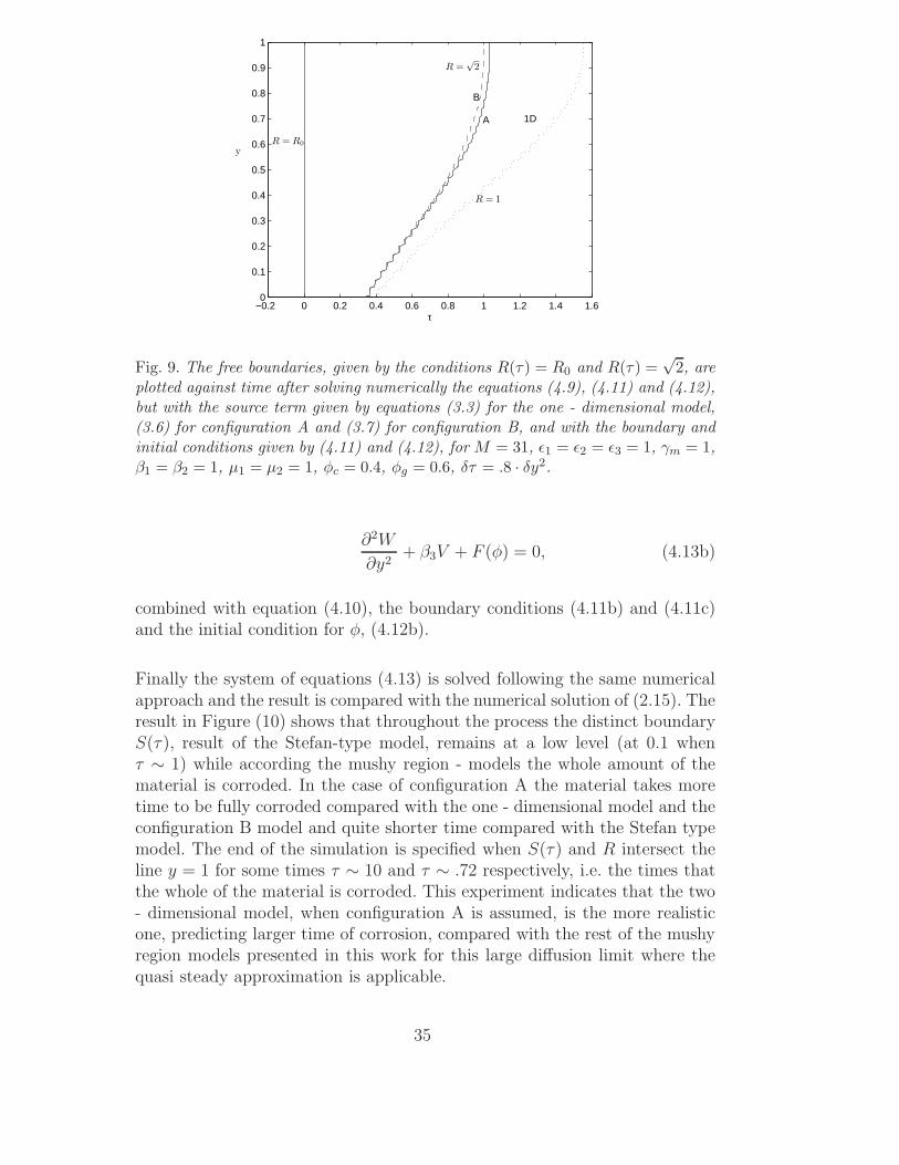
Finally the system of equations (4.13) is solved following the same numericalapproach and the result is compared with the numerical solution of (2.15). Theresult in Figure (10) shows that throughout the process the distinct boundaryS(τ), result of the Stefan-type model, remains at a low level (at 0.1 whenτ ∼ 1) while according the mushy region - models the whole amount of thematerial is corroded. In the case of configuration A the material takes moretime to be fully corroded compared with the one - dimensional model and theconfiguration B model and quite shorter time compared with the Stefan typemodel. The end of the simulation is specified when S(τ) and R intersect theline y = 1 for some times τ ∼ 10 and τ ∼ .72 respectively, i.e. the times thatthe whole of the material is corroded. This experiment indicates that the two- dimensional model, when configuration A is assumed, is the more realisticone, predicting larger time of corrosion, compared with the rest of the mushyregion models presented in this work for this large diffusion limit where thequasi steady approximation is applicable.

35

0 0.2 0.4 0.6 0.8 10

0.1

0.2

0.3

0.4

0.5

0.6

0.7

0.8

0.9

1

BR(τ ) =

√2

1DR(τ ) = 1 A

R(τ ) =√

2

S(τ )

y

τ

R(τ ) = R0

Fig. 10. The free boundaries, given by the conditions R(y, τ) = R0 and R(y, τ) =√

2,and S(τ) are plotted against time after solving numerically the equations (4.9),(4.11) and (4.12), but with the source term given by equations (3.3) for the one- dimensional model, (3.6) for configuration A and (3.7) for configuration B, andwith S(τ) given by (2.15). The boundary and initial conditions for the mushy regionmodels are given by (4.11b, 4.11c ), the last two of (4.12a) and (4.12b). The valuesof the parameters that were used were M = 31, δ = 0.1, γm = 6.78, γ = 67.8β2 = 2.3275, β3 = 2.3741 10−5, φc = 0.2, φg = 0.3 δτ = 0.4 · δy2.

5 Conclusions

In this work a mathematical model for the formation of a mushy region duringcorrosion by H2SO4 is constructed. The model is based in an already existingmodel for the corrosion of sewer pipes resulting in a Stefan problem. For thisStefan problem although an extensive analysis has been done in a series ofpapers by Bohm et all in [4] etc, an approximate solution is presented for acertain range of values of parameters corresponding to real situations as it ismentioned in [4]. The result is in very good agreement with these from [4].

As a next step a model is constructed allowing the formation of a mushy re-gion, i.e. a region where the material is only partly corroded throughout theprocess. This more general model is derived via an averaging process of mi-croscopic considerations, by the application of a method presented in [13] andhas the form of a macroscopic phase field model. Variations of this model arepresented in the case of a one - dimensional and two - dimensional consider-ations regarding the geometry of the cracks inside the concrete. The derivedphase field models in their various forms, are solved numerically with a finiteelement scheme and the results, which predict corrosion within a reasonablerange, are presented.

36

More complicated considerations of the geometry of cracks as well as theirfractal structure, can be taken into account and lead to more realistic models.Furthermore other models accounting for the corrosion of the calcite nearpossible intersections of pores can be derived based on a combination of theone-dimensional model regarding corrosion away from the intersections anda two-dimensional model for the corrosion near the intersections. In additionvariations of the scaling used in the multiple scales approach, for examplewhen γm is not of order one, may result in interesting future extensions of thiswork.

References

[1] G. Ali, V. Furuholt, R. Natalini, I. Torcicollo, A mathematical model ofsulphite chemical aggression of limestones with high permeability. I. Modelingand qualitative analysis. Transp. Porous Media 69, no. 1, (2007), 109–122.

[2] G. Ali, V. Furuholt, R. Natalini, I. Torcicollo, A mathematical model ofsulphite chemical aggression of limestones with high permeability. II. Numericalapproximation. Transp. Porous Media 69, no. 2, (2007), 175–188.

[3] N. De Belie, J. Montenya, A. Beeldensb, E. Vinckec, D. Van Gemertb,W.Verstraetec Experimental research and prediction of the effect of chemical andbiogenic sulfuric acid on different types of commercially produced concrete sewerpipes, Cement and Concrete Research, 34, no 12, (2004), 2223–2236.

[4] M. Bohm, J. Devinny, F. Jahani, G. Rosen, On a moving-boundary systemmodelling corrosion in sewer pipes, Applied Mathematics and Computation, 92,(1998), 247–269.

[5] M. Bohm, J. S. Devinny, F. Jahani, F. B. Mansfeld, I. G. Rosen, C.Wang, AMoving Boundary Diffusion Model for the Corrosion of Concrete WastewaterSystems: Simulation and Experimental Validation, Proceedings of the ArnencanControl Conference San Diego, California, June 1999, 1739–1743.

[6] A. M. Brandt, G. Prokopski, On the fractal dimension of fracture surfaces ofconcrete elements, Journal of Materials Science, 28, no 17, (1993), 4762–4766.

[7] B Chiaia, J. G. M. van Mier, A. Vervuurt, On the fractal dimension of fracturesurfaces of concrete elements, Cement and Concrete Research, 28, no 1, (1998),103–114.

[8] A. Fasano, R. Natalini Lost Beauties of the Acropolis : What Mathematics CanSay, SIAM News, 39, July/August 2006.

[9] C. Giavarini, M. L. Santarelli, R. Natalini, and F. Freddi, A nonlinear model ofsulfa- tion of porous stones: Numerical simulations and preliminary laboratoryassessments J. Cultural Heritage, 9, (2008), 14–22.

37

[10] F.R. Guargualini, R. Natalini Global Existence of solutions to a nonlinear modelof sulphasion phenomena in calcium carbonate stones, Nonlinear Analysis : RealWorld Applications, 6, (2005), 477–494.

[11] G. M. Idorn Innovation in concrete researchreview and perspective,Cement andConcrete Research, 35, (2005), 3–10.

[12] A. Muntean, M. Bohm, A moving-boundary problem for concrete carbonation:global existence and uniqueness of weak solutions. J. Math. Anal. Appl. 350, no.1, (2009), 234–251.

[13] A.A Lacey, L.A. Herraiz Macroscopic models for melting derived from averagingmicroscopic Stefan problems I: Simple geometries with kinetic undercooling orsurface tension . Euro. Jnl. of Applied Mathematics, 11, (2002), 153–169.

[14] A.A Lacey, L.A. Herraiz Macroscopic models for melting derived from averagingmicroscopic Stefan problems II: Effect of Varying geometry and composition.Euro. Jnl. of Applied Mathematics, 13, (2002), 261–282.

38