Prof. Dr. Barbara Wohlmuth

Lehrstuhl fur Numerische Mathematik

Definition A-stabil

Wir betrachen das Modellproblem:

y′(t) = λy(t)

y(0) = 1fur λ ∈ C, mit Re(λ) < 0

• Ein Verfahren heißt absolut stabil, falls limi→∞ |yi| = 0.

• Sei yi+1 = R(z)yi, z = hλ, dann die R(z) heißt Stabilitatsfunktion.

• Das Stabilitatsgebiet A ist definiert als

A :=

hλ ∈ C : limi→∞

|yi| = 0,

=

z ∈ C : |R(z)| < 1

,

d.h. die approximative und analytische Losungen haben gleiche asymptotischeEigenschaften.

• Ein Verfahren heißt A-stabil, falls C− ⊂ A

– Typeset by FoilTEX – 1

Prof. Dr. Barbara Wohlmuth

Lehrstuhl fur Numerische Mathematik

Stabilitatsgebiete A

-3 -2 -1 0 1 2 3

x

-3

-2

-1

0

1

2

3

yExplicit Euler

-3 -2 -1 0 1 2 3

x

-3

-2

-1

0

1

2

3

y

Heun

-3 -2 -1 0 1 2 3

x

-3

-2

-1

0

1

2

3

y

Implicit Euler

-3 -2 -1 0 1 2 3

x

-3

-2

-1

0

1

2

3

y

Crank-Nicolson

– Typeset by FoilTEX – 2

Prof. Dr. Barbara Wohlmuth

Lehrstuhl fur Numerische Mathematik

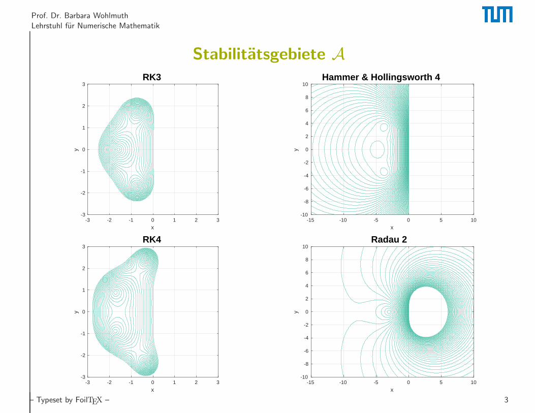
Stabilitatsgebiete A

-3 -2 -1 0 1 2 3

x

-3

-2

-1

0

1

2

3

yRK3

-3 -2 -1 0 1 2 3

x

-3

-2

-1

0

1

2

3

y

RK4

-15 -10 -5 0 5 10

x

-10

-8

-6

-4

-2

0

2

4

6

8

10

y

Hammer & Hollingsworth 4

-15 -10 -5 0 5 10

x

-10

-8

-6

-4

-2

0

2

4

6

8

10

y

Radau 2

– Typeset by FoilTEX – 3

Prof. Dr. Barbara Wohlmuth

Lehrstuhl fur Numerische Mathematik

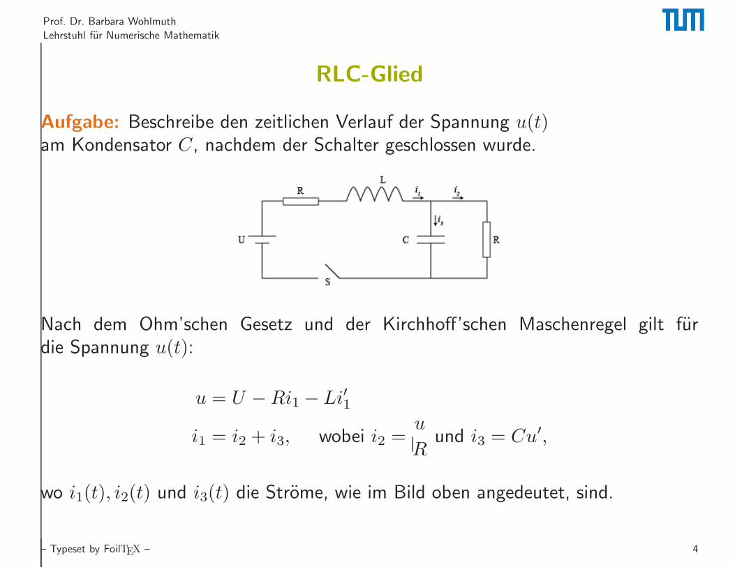
RLC-Glied

Aufgabe: Beschreibe den zeitlichen Verlauf der Spannung u(t)am Kondensator C, nachdem der Schalter geschlossen wurde.

Nach dem Ohm’schen Gesetz und der Kirchhoff’schen Maschenregel gilt furdie Spannung u(t):

u = U −Ri1 − Li′1

i1 = i2 + i3, wobei i2 =u

Rund i3 = Cu′,

wo i1(t), i2(t) und i3(t) die Strome, wie im Bild oben angedeutet, sind.

– Typeset by FoilTEX – 4

Prof. Dr. Barbara Wohlmuth

Lehrstuhl fur Numerische Mathematik

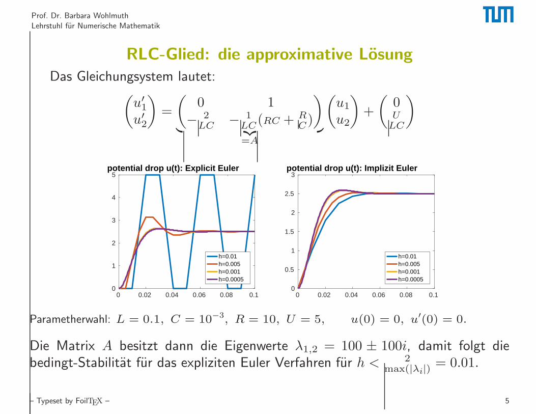
RLC-Glied: die approximative Losung

Das Gleichungsystem lautet:(u′1

u′2

)

=

(0 1

− 2LC

− 1LC

(RC + RC)

)

︸ ︷︷ ︸=A

(u1

u2

)

+

(0ULC

)

0 0.02 0.04 0.06 0.08 0.10

1

2

3

4

5potential drop u(t): Explicit Euler

h=0.01h=0.005h=0.001h=0.0005

0 0.02 0.04 0.06 0.08 0.10

0.5

1

1.5

2

2.5

3potential drop u(t): Implizit Euler

h=0.01h=0.005h=0.001h=0.0005

Parametherwahl: L = 0.1, C = 10−3, R = 10, U = 5, u(0) = 0, u′(0) = 0.

Die Matrix A besitzt dann die Eigenwerte λ1,2 = 100 ± 100i, damit folgt diebedingt-Stabilitat fur das expliziten Euler Verfahren fur h < 2

max(|λi|)= 0.01.

– Typeset by FoilTEX – 5

Prof. Dr. Barbara Wohlmuth

Lehrstuhl fur Numerische Mathematik

Definition L-stabil

Obwohl das Verfahren A-stabil ist, konnen lokale Oszilationen in der approximativenLosung auftreten.

Ein RKV heißt L-stabil, falls es A-stabil ist und zusatzlich gilt:

lim|z|→∞

R(z) = 0.

Bemerkung:

Explizite RKV konnen dann auch nicht L-stabil sein.Fur implizite RKV mit R(z) = P (z)

Q(z) muss gelten: deg(P ) < deg(Q).

– Typeset by FoilTEX – 6

Prof. Dr. Barbara Wohlmuth

Lehrstuhl fur Numerische Mathematik

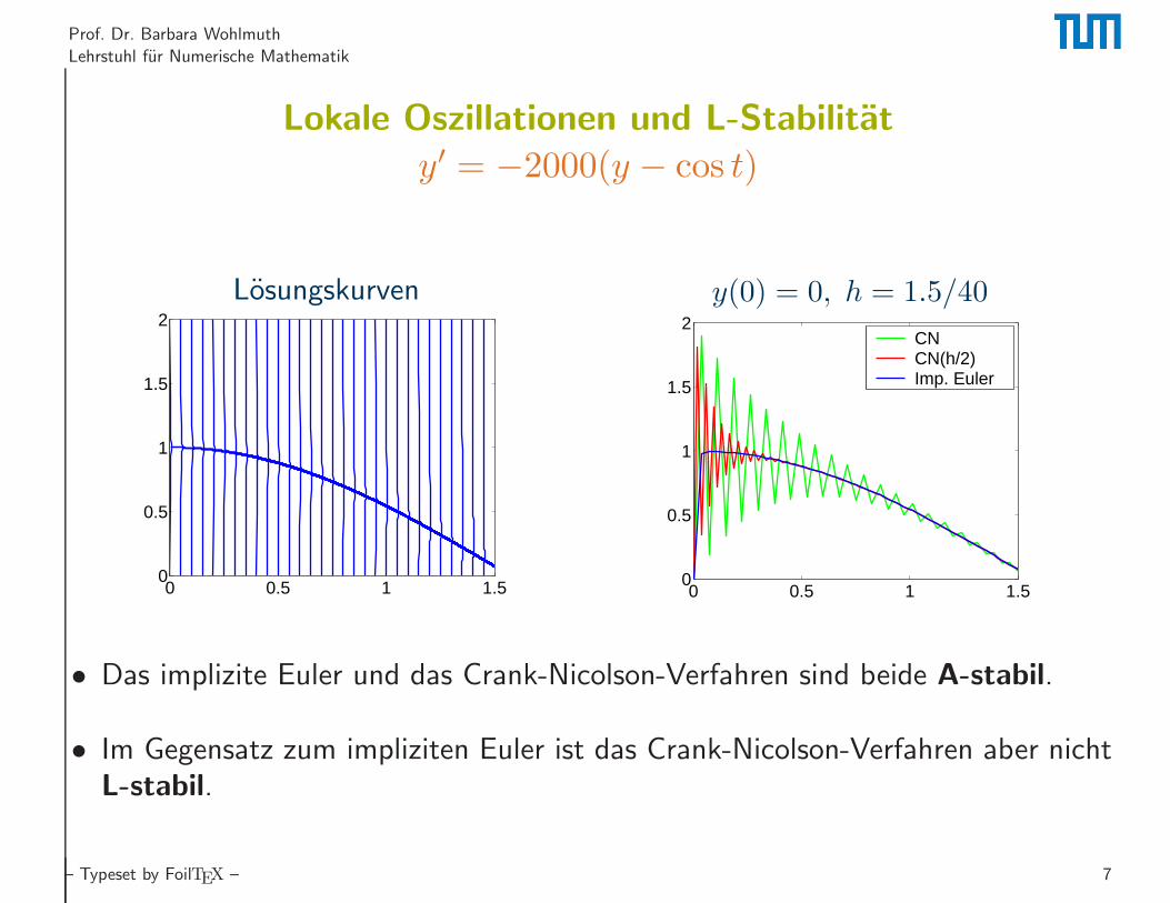
Lokale Oszillationen und L-Stabilitat

y′ = −2000(y − cos t)

Losungskurven

0 0.5 1 1.50

0.5

1

1.5

2y(0) = 0, h = 1.5/40

0 0.5 1 1.50

0.5

1

1.5

2CNCN(h/2)Imp. Euler

• Das implizite Euler und das Crank-Nicolson-Verfahren sind beide A-stabil.

• Im Gegensatz zum impliziten Euler ist das Crank-Nicolson-Verfahren aber nichtL-stabil.

– Typeset by FoilTEX – 7

Prof. Dr. Barbara Wohlmuth

Lehrstuhl fur Numerische Mathematik

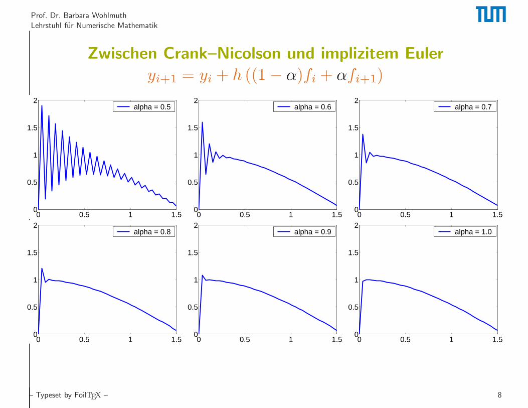
Zwischen Crank–Nicolson und implizitem Euler

yi+1 = yi + h ((1− α)fi + αfi+1)

0 0.5 1 1.50

0.5

1

1.5

2alpha = 0.5

0 0.5 1 1.50

0.5

1

1.5

2alpha = 0.6

0 0.5 1 1.50

0.5

1

1.5

2alpha = 0.7

0 0.5 1 1.50

0.5

1

1.5

2alpha = 0.8

0 0.5 1 1.50

0.5

1

1.5

2alpha = 0.9

0 0.5 1 1.50

0.5

1

1.5

2alpha = 1.0

– Typeset by FoilTEX – 8

Prof. Dr. Barbara Wohlmuth

Lehrstuhl fur Numerische Mathematik

Definition B-stabil

• Sei f : Ω → Rd, Ω ⊂ R

d, f heißt streng dissipativ, falls

〈f(y)− f(y), y − y〉 < 0, ∀y, y ∈ Ω.

• Wendet man ein RKV auf ein AWP mit dissipativer rechter Seite an, so heißtdieses RKV B-stabil, falls fur h > 0 folgt:

‖y1 − y1‖ 6 ‖y0 − y0‖ ,

wobei y1 := y0 + hΦ(t0, h, y0, y1) und y1 := y0 + hΦ(t0, h, y0, y1) und Φ dieVerfahrensfunktion des RKV ist.

Bemerkung: B-stabile Verfahren sind auch A-stabil.Bei dissipativen Systemen nimmt also der Einfluß einer kleinen Storung in den ABnicht mit der Zeit zu.

– Typeset by FoilTEX – 9

Prof. Dr. Barbara Wohlmuth

Lehrstuhl fur Numerische Mathematik

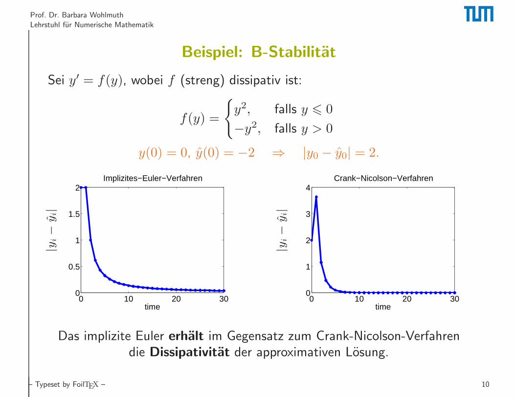
Beispiel: B-Stabilitat

Sei y′ = f(y), wobei f (streng) dissipativ ist:

f(y) =

y2, falls y 6 0

−y2, falls y > 0

y(0) = 0, y(0) = −2 ⇒ |y0 − y0| = 2.

|yi−

yi|

0 10 20 300

0.5

1

1.5

2

time

Implizites−Euler−Verfahren

|yi−

yi|

0 10 20 300

1

2

3

4

time

Crank−Nicolson−Verfahren

Das implizite Euler erhalt im Gegensatz zum Crank-Nicolson-Verfahrendie Dissipativitat der approximativen Losung.

– Typeset by FoilTEX – 10

Prof. Dr. Barbara Wohlmuth

Lehrstuhl fur Numerische Mathematik

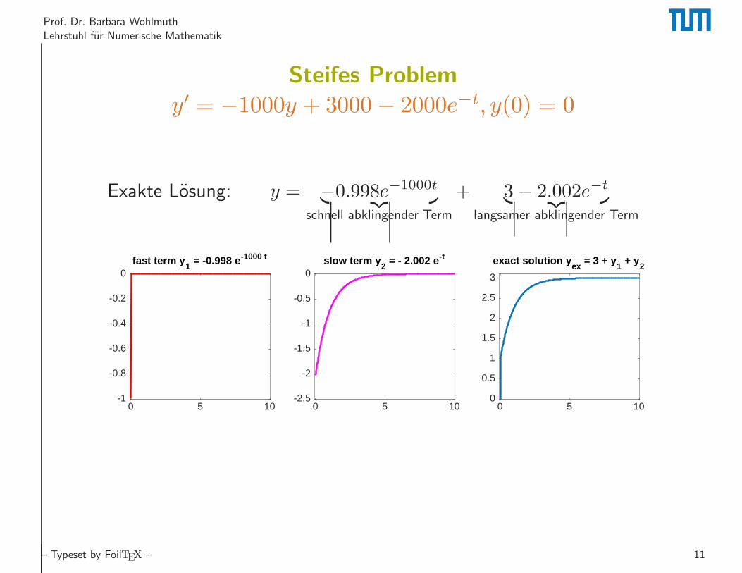
Steifes Problem

y′ = −1000y + 3000− 2000e−t, y(0) = 0

Exakte Losung: y = −0.998e−1000t︸ ︷︷ ︸

schnell abklingender Term

+ 3− 2.002e−t︸ ︷︷ ︸

langsamer abklingender Term

0 5 10-1

-0.8

-0.6

-0.4

-0.2

0fast term y

1 = -0.998 e-1000 t

0 5 10-2.5

-2

-1.5

-1

-0.5

0slow term y

2 = - 2.002 e-t

0 5 100

0.5

1

1.5

2

2.5

3

exact solution yex

= 3 + y1 + y

2

– Typeset by FoilTEX – 11

Prof. Dr. Barbara Wohlmuth

Lehrstuhl fur Numerische Mathematik

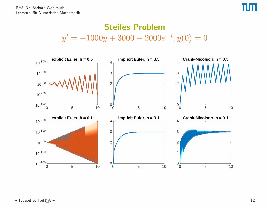
Steifes Problem

y′ = −1000y + 3000− 2000e−t, y(0) = 0

0 5 1010-100

10 -50

10 0

10 50

10 100explicit Euler, h = 0.5

0 5 100

1

2

3

4implicit Euler, h = 0.5

0 5 100

1

2

3

4Crank-Nicolson, h = 0.5

0 5 1010-200

10-100

10 0

10 100

10 200explicit Euler, h = 0.1

0 5 100

1

2

3

4implicit Euler, h = 0.1

0 5 100

1

2

3

4Crank-Nicolson, h = 0.1

– Typeset by FoilTEX – 12

Prof. Dr. Barbara Wohlmuth

Lehrstuhl fur Numerische Mathematik

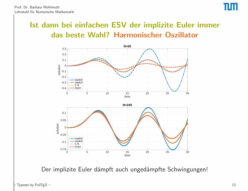
Ist dann bei einfachen ESV der implizite Euler immer

das beste Wahl? Harmonischer Oszillator

0 5 10 15 20 25 30time

-0.4

-0.3

-0.2

-0.1

0

0.1

0.2

0.3

solu

tion

N=60

explicitimplicitC-Nexact

0 5 10 15 20 25 30time

-0.15

-0.1

-0.05

0

0.05

0.1

solu

tion

N=240

explicitimplicitC-Nexact

Der implizite Euler dampft auch ungedampfte Schwingungen!

– Typeset by FoilTEX – 13