Curse of Dimensionality, Dimensionality Reduction with …rita/uml_course/add_mat/PCA.pdf · Curse...

Curse of Dimensionality, Dimensionality Reduction with PCA

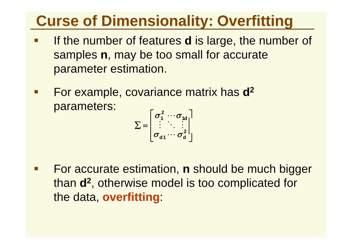
Curse of Dimensionality: Overfitting� If the number of features d is large, the number of

samples n, may be too small for accurate parameter estimation.

� For example, covariance matrix has d2

parameters:

====∑∑∑∑1

21 dσσσσσσσσ

MOM

L

====∑∑∑∑2

1 dd σσσσσσσσ L

MOM

� For accurate estimation, n should be much bigger than d2, otherwise model is too complicated for the data, overfitting:

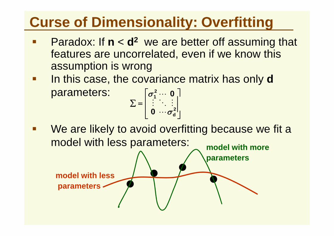
� Paradox: If n < d2 we are better off assuming that features are uncorrelated, even if we know this assumption is wrong

� In this case, the covariance matrix has only dparameters:

====∑∑∑∑

2

21

0

0

dσσσσ

σσσσ

L

MOM

L

Curse of Dimensionality: Overfitting

� We are likely to avoid overfitting because we fit a model with less parameters: model with more

parameters

model with lessparameters

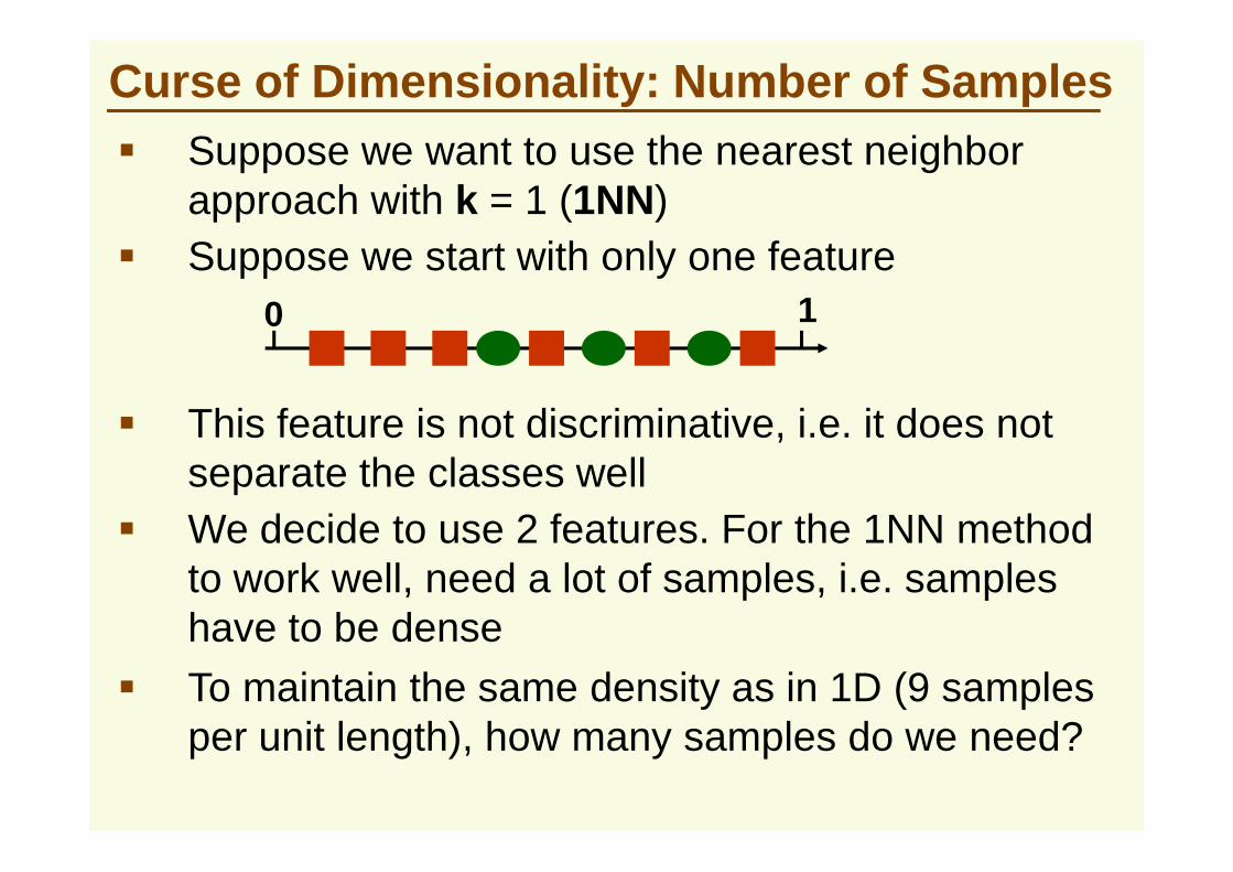
Curse of Dimensionality: Number of Samples� Suppose we want to use the nearest neighbor

approach with k = 1 (1NN)

� This feature is not discriminative, i.e. it does not

� Suppose we start with only one feature0 1

� This feature is not discriminative, i.e. it does not separate the classes well

� We decide to use 2 features. For the 1NN method to work well, need a lot of samples, i.e. samples have to be dense

� To maintain the same density as in 1D (9 samples per unit length), how many samples do we need?

Curse of Dimensionality: Number of Samples

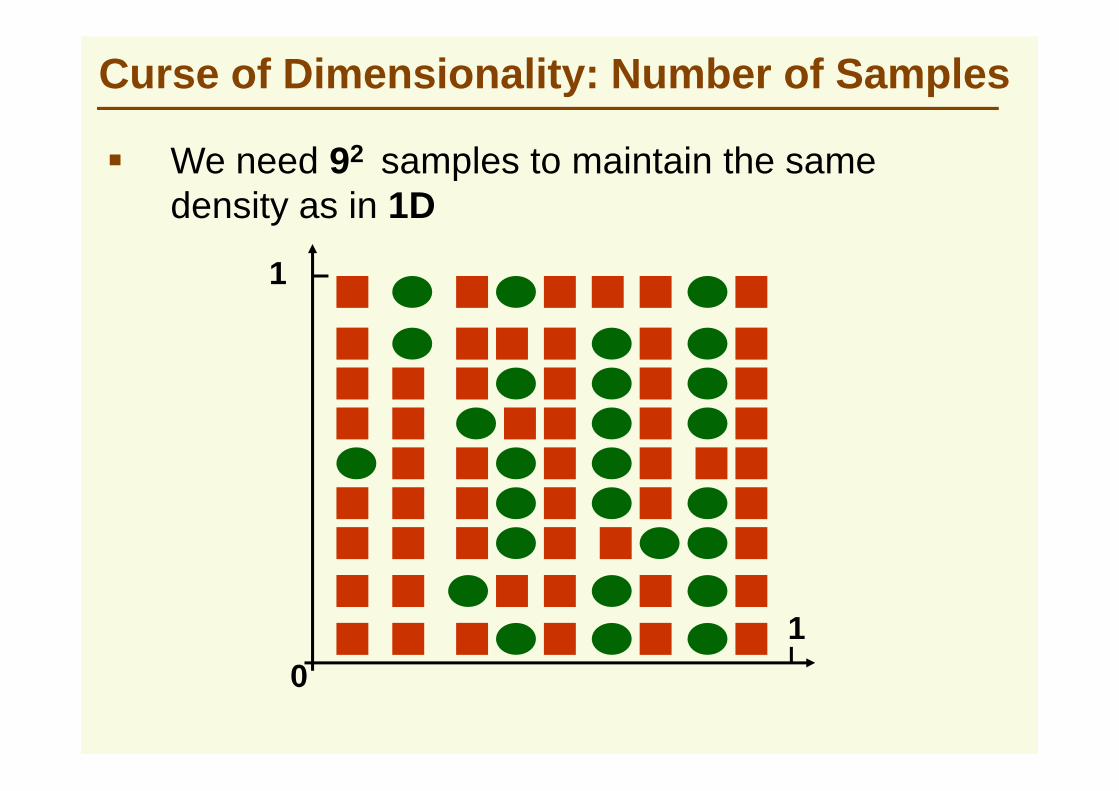
� We need 92 samples to maintain the same density as in 1D

1

0

1

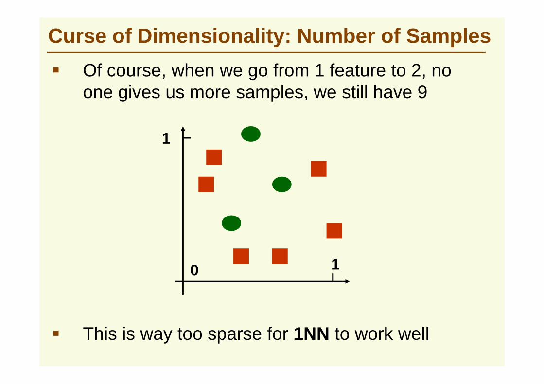
� Of course, when we go from 1 feature to 2, no one gives us more samples, we still have 9

1


0 1

� This is way too sparse for 1NN to work well

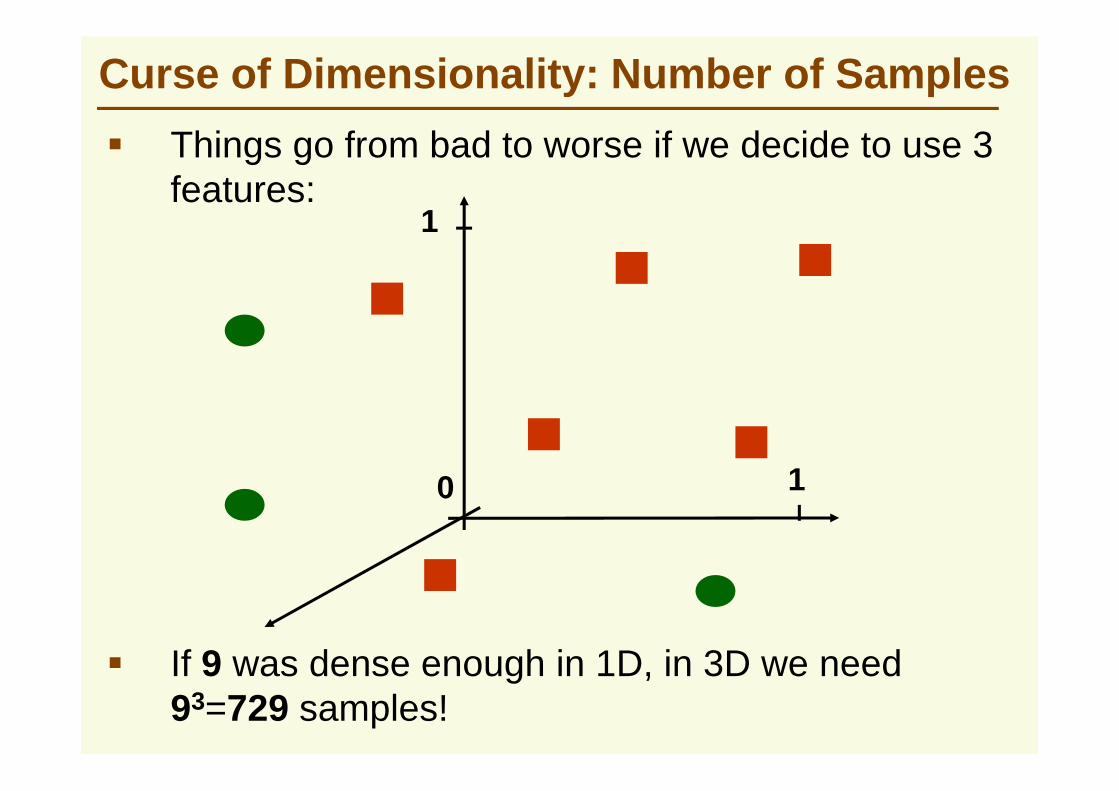
� Things go from bad to worse if we decide to use 3 features:

1


0 1

� If 9 was dense enough in 1D, in 3D we need 93=729 samples!

� In general, if n samples is dense enough in 1D

� Then in d dimensions we need nd samples!

� And nd grows really really fast as a function of d

� Common pitfall:


� Common pitfall:� If we can’t solve a problem with a few features, adding

more features seems like a good idea� However the number of samples usually stays the same� The method with more features is likely to perform

worse instead of expected better

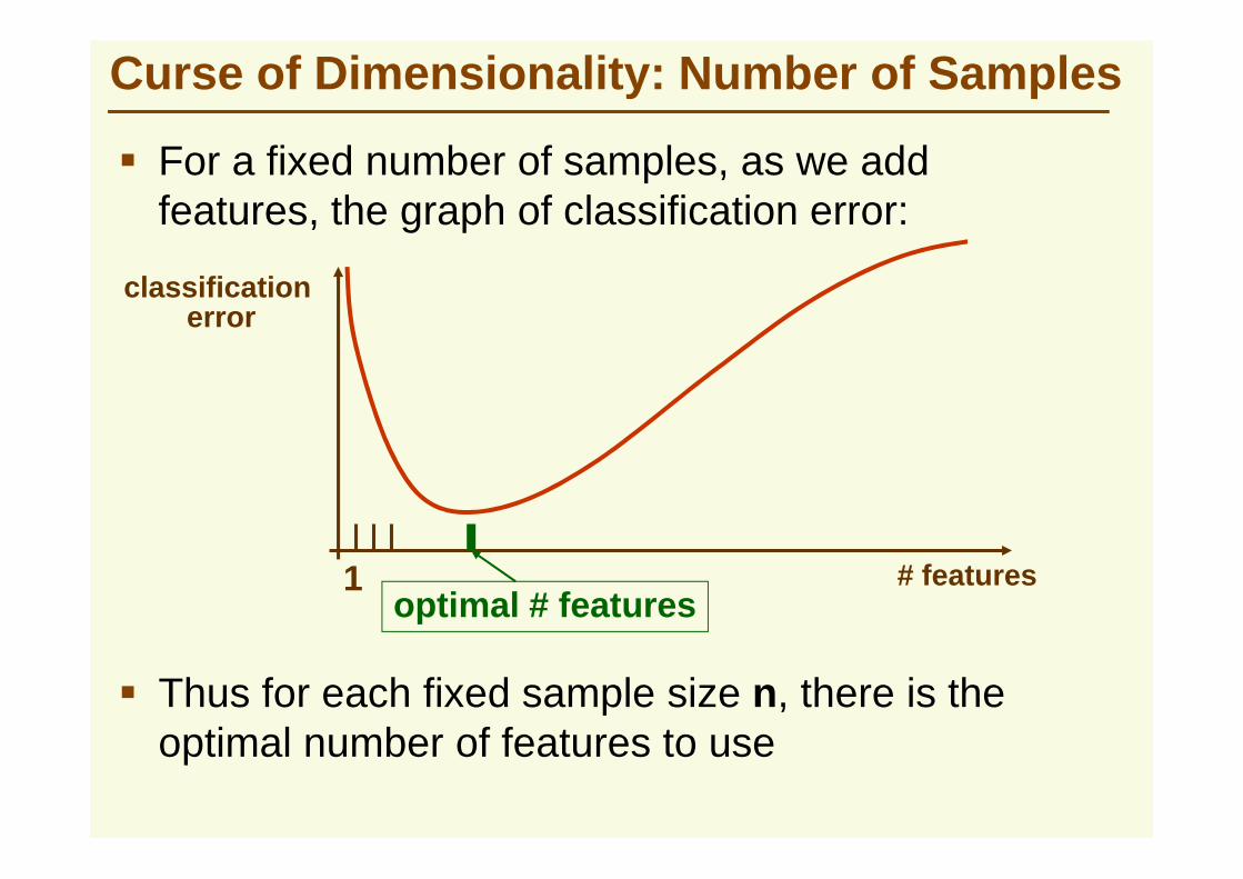
� For a fixed number of samples, as we add features, the graph of classification error:

classification error


# features1optimal # features

� Thus for each fixed sample size n, there is the optimal number of features to use

� We should try to avoid creating lot of features

The Curse of Dimensionality

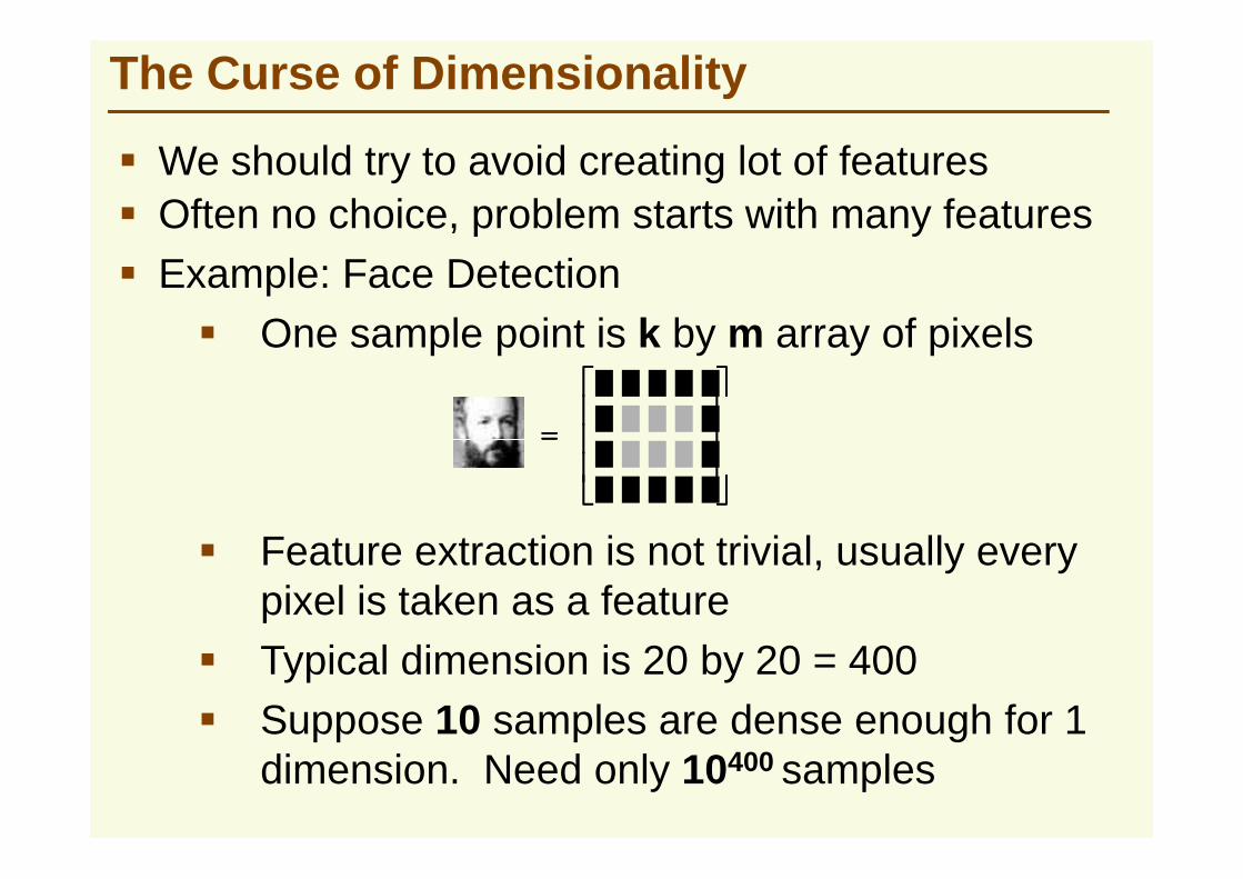
� Often no choice, problem starts with many features� Example: Face Detection

� One sample point is k by m array of pixels

====

====

� Feature extraction is not trivial, usually every pixel is taken as a feature

� Typical dimension is 20 by 20 = 400� Suppose 10 samples are dense enough for 1

dimension. Need only 10400 samples

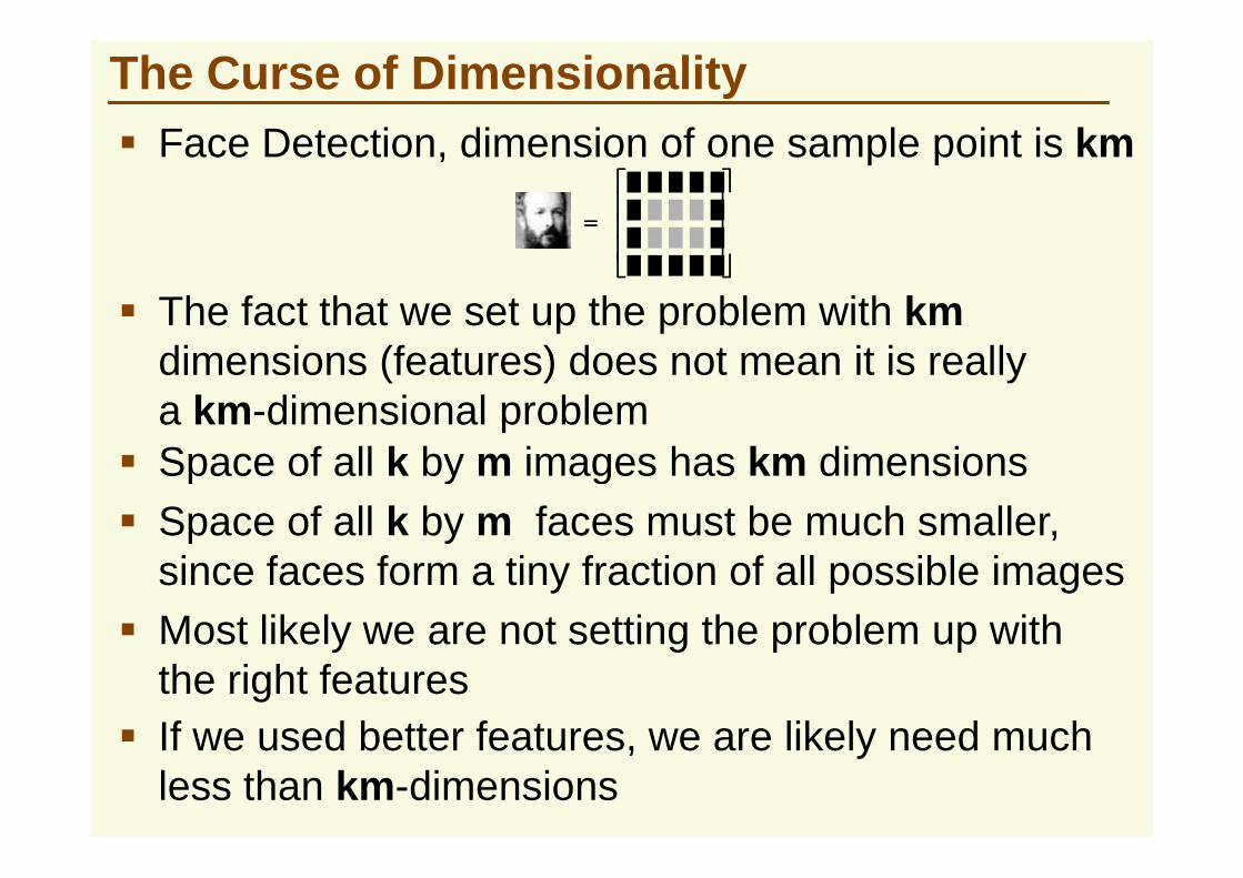
The Curse of Dimensionality� Face Detection, dimension of one sample point is km

====

� The fact that we set up the problem with kmdimensions (features) does not mean it is really a km-dimensional problem

� Space of all k by m images has km dimensions

� Most likely we are not setting the problem up with the right features

� If we used better features, we are likely need much less than km-dimensions

� Space of all k by m images has km dimensions� Space of all k by m faces must be much smaller,

since faces form a tiny fraction of all possible images

Dimensionality Reduction

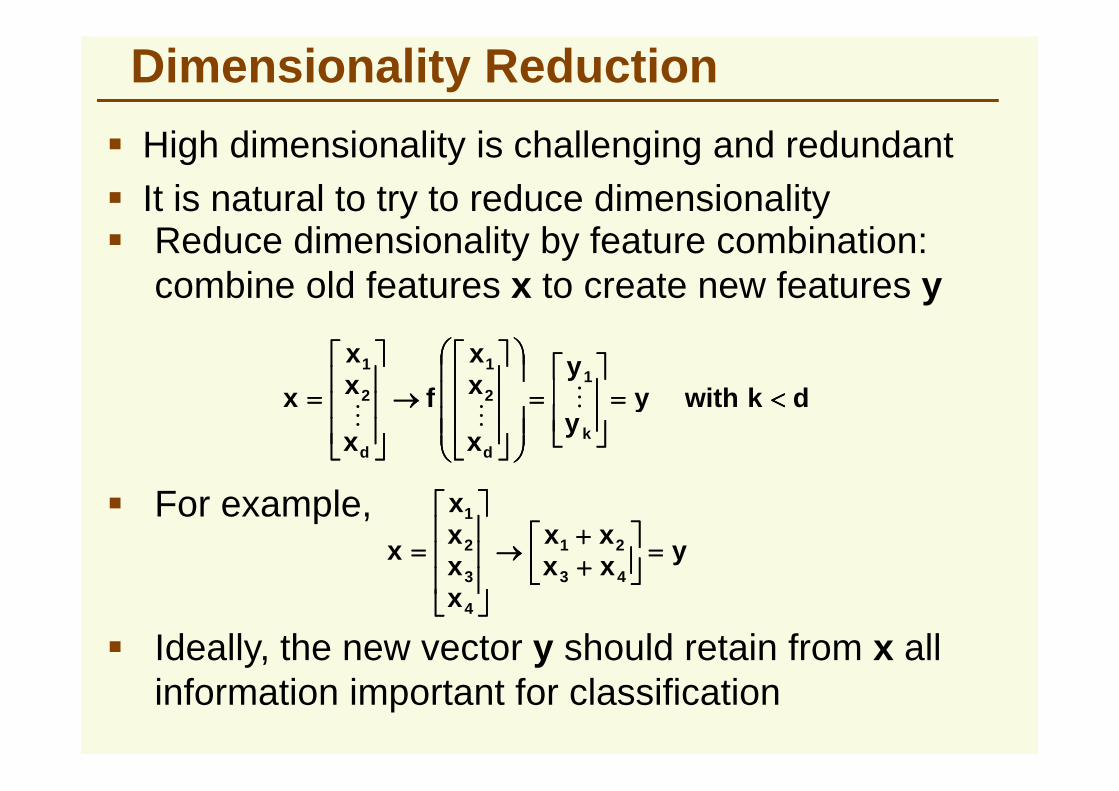
� High dimensionality is challenging and redundant� It is natural to try to reduce dimensionality� Reduce dimensionality by feature combination:

combine old features x to create new features y

dkwithyy

xx

fxx

x <<<<====

====

→→→→

==== M1

2

1

2

1

yxxxx

xxxx

x43

21

4

3

2

1

====

++++++++

→→→→

====

dkwithyy

x

xf

x

xxk

dd

<<<<====

====

→→→→

==== MMM22

� For example,

� Ideally, the new vector y should retain from x all information important for classification

Dimensionality Reduction

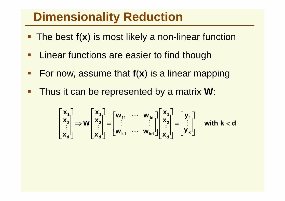
� The best f(x) is most likely a non-linear function

� Linear functions are easier to find though

� Thus it can be represented by a matrix W:

� For now, assume that f(x) is a linear mapping

dkwithy

y

x

xx

ww

ww

x

xx

W

x

xx

kd

kdk

d

dd

<<<<

====

====

⇒⇒⇒⇒

MM

L

MM

L

MM

12

1

1

1112

1

2

1

� We will look at 2 methods for feature combination� Principle Component Analysis (PCA)� Fischer Linear Discriminant (next lecture)

Feature Combination

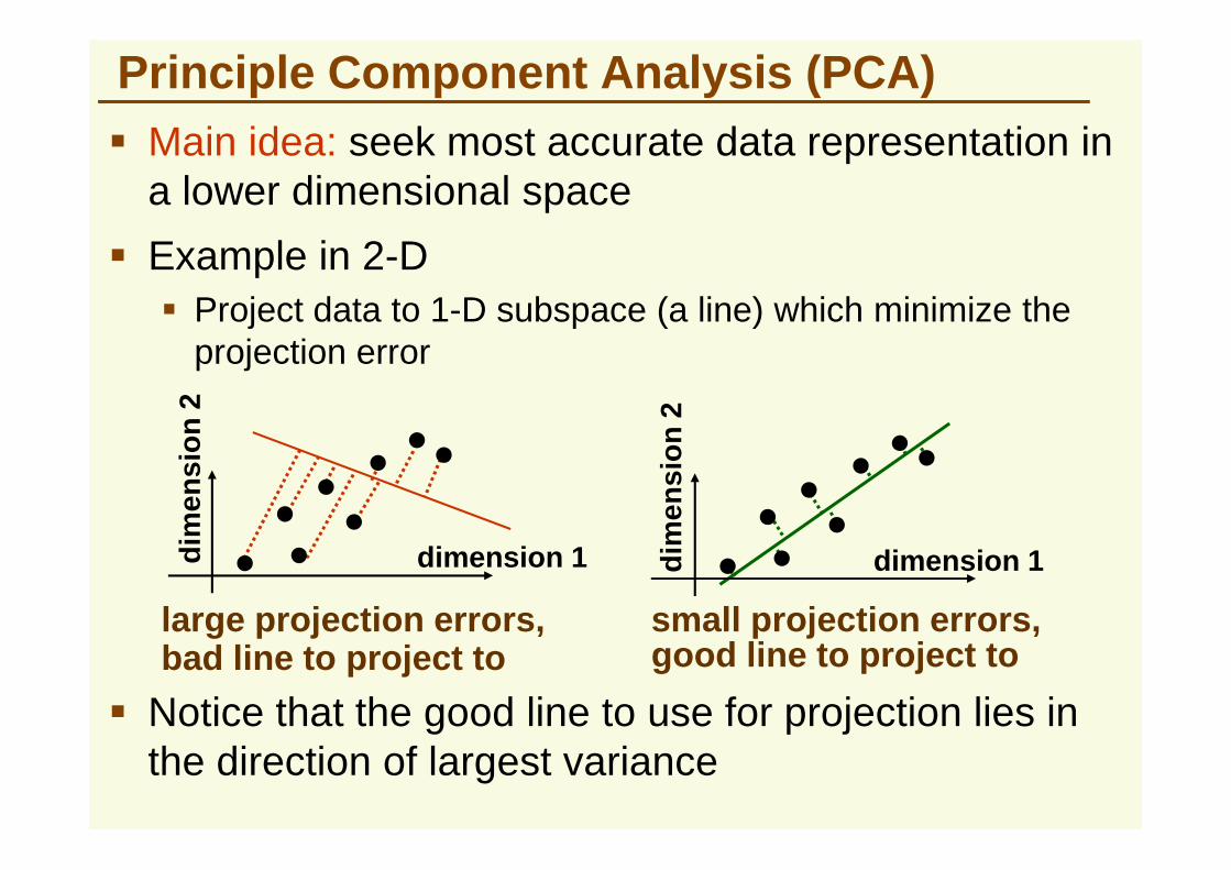
� Main idea: seek most accurate data representation in a lower dimensional space

Principle Component Analysis (PCA)

� Example in 2-D� Project data to 1-D subspace (a line) which minimize the

projection error

dim

ensi

on

2

dim

ensi

on

2

large projection errors,bad line to project to

small projection errors,good line to project to

dimension 1dim

ensi

on

dimension 1dim

ensi

on

� Notice that the good line to use for projection lies in the direction of largest variance

PCA

y

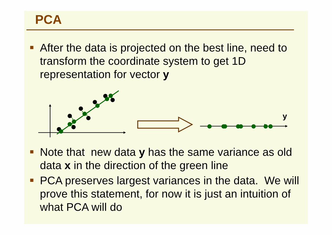
� After the data is projected on the best line, need to transform the coordinate system to get 1D representation for vector y

y

� Note that new data y has the same variance as old data x in the direction of the green line

� PCA preserves largest variances in the data. We will prove this statement, for now it is just an intuition of what PCA will do

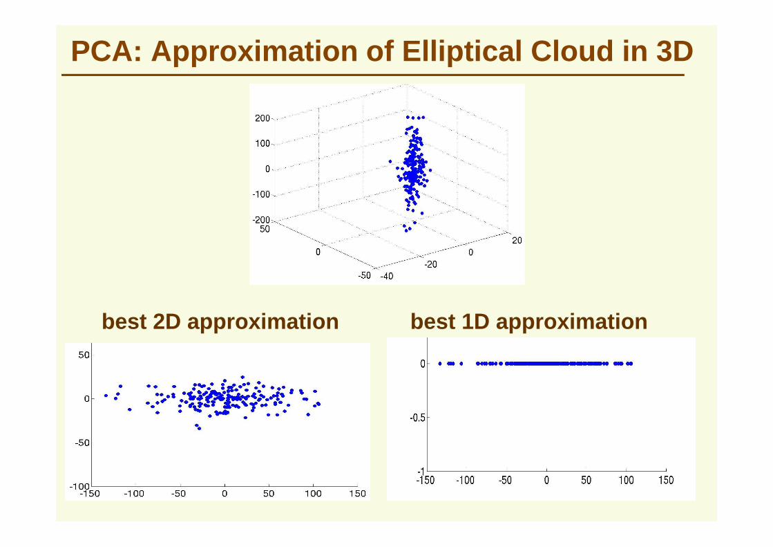
PCA: Approximation of Elliptical Cloud in 3D

best 2D approximation best 1D approximation

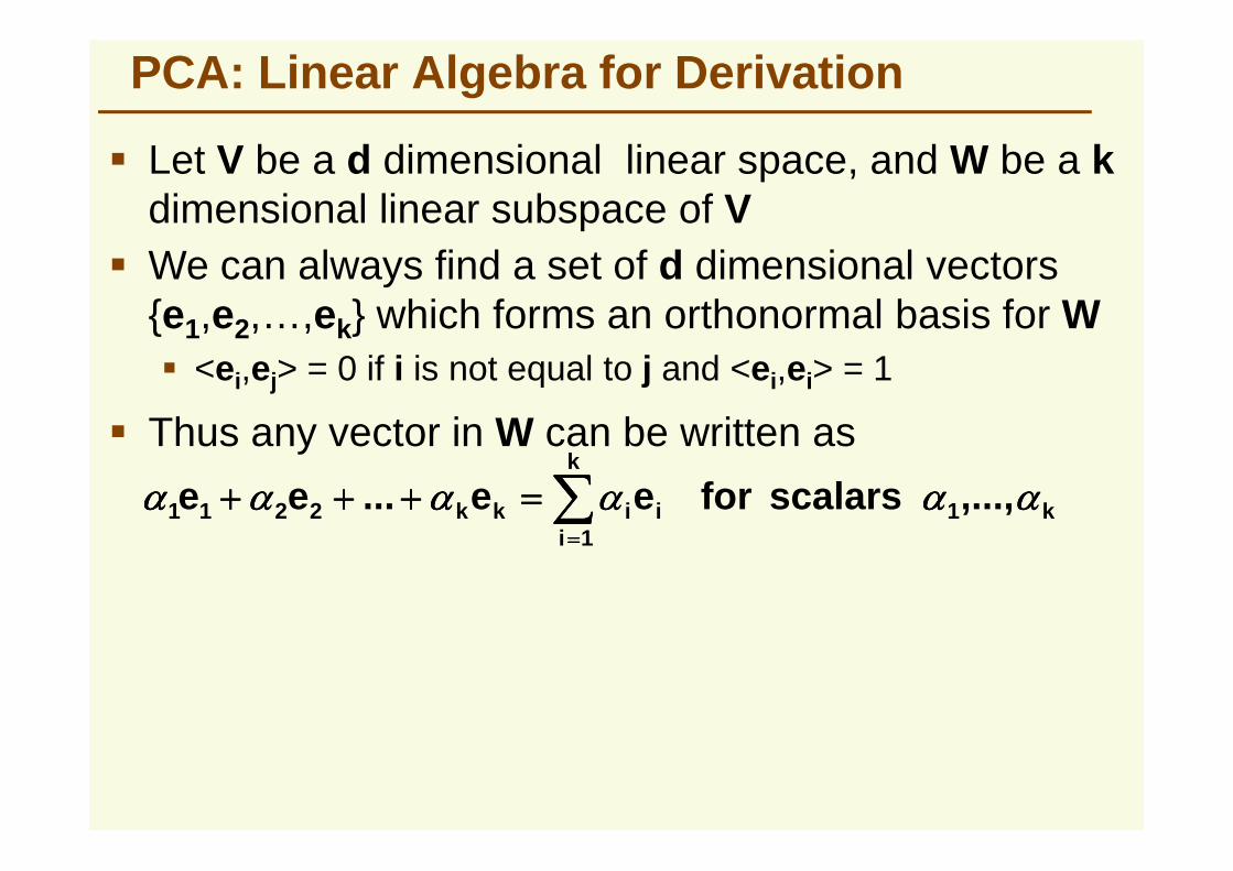
PCA: Linear Algebra for Derivation

� Let V be a d dimensional linear space, and W be a kdimensional linear subspace of V

� We can always find a set of d dimensional vectors {e1,e2,…,ek} which forms an orthonormal basis for W� <ei,ej> = 0 if i is not equal to j and <ei,ei> = 1

� Thus any vector in W can be written as � Thus any vector in W can be written as

k

k

iiikk scalarsforeeee αααααααααααααααααααααααα ,...,... 1

12211 ∑∑∑∑

====

====++++++++++++

PCA: Linear Algebra for Derivation

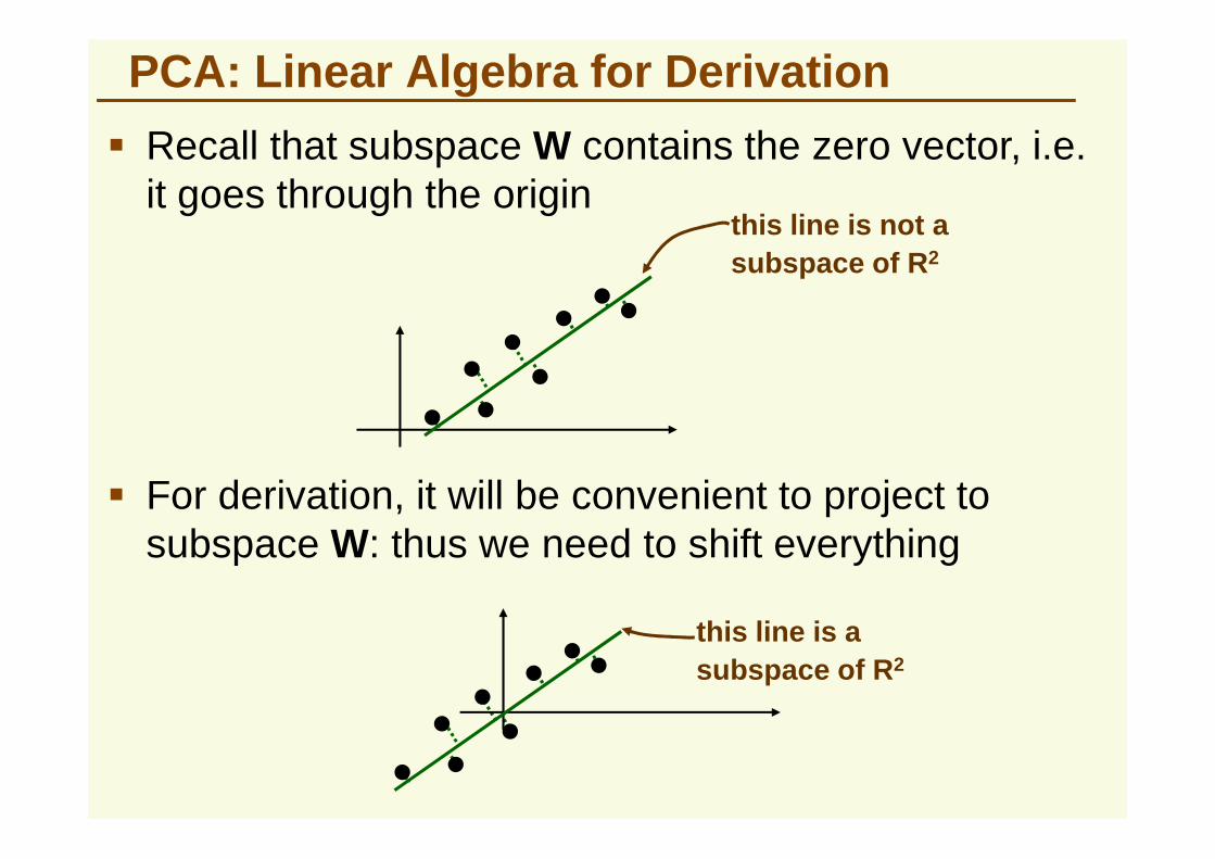
� Recall that subspace W contains the zero vector, i.e. it goes through the origin

this line is not a subspace of R2

� For derivation, it will be convenient to project to subspace W: thus we need to shift everything

this line is a subspace of R2

PCA Derivation: Shift by the Mean Vector

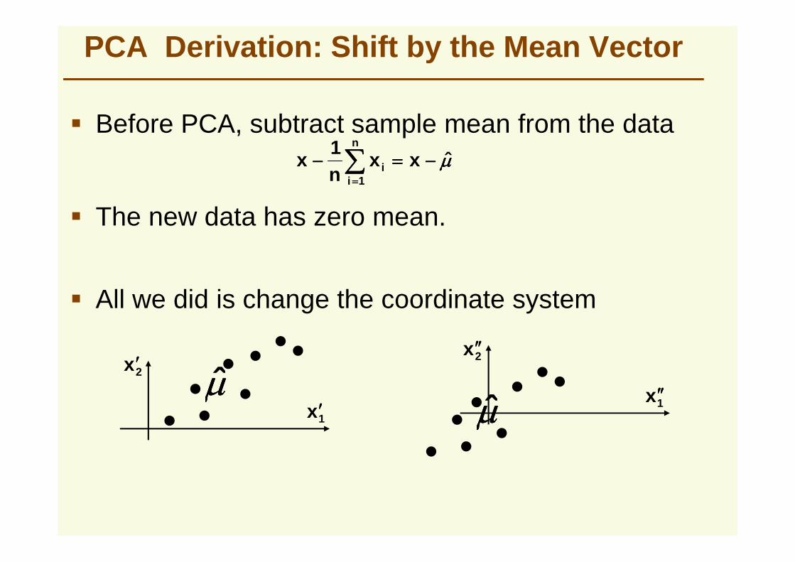
� Before PCA, subtract sample mean from the dataµµµµ̂

1

1

−−−−====−−−− ∑∑∑∑====

xxn

xn

ii

� The new data has zero mean.

1x ′′′′

2x ′′′′

1x ′′′′′′′′

2x ′′′′′′′′

µµµµ̂µµµµ̂

� All we did is change the coordinate system

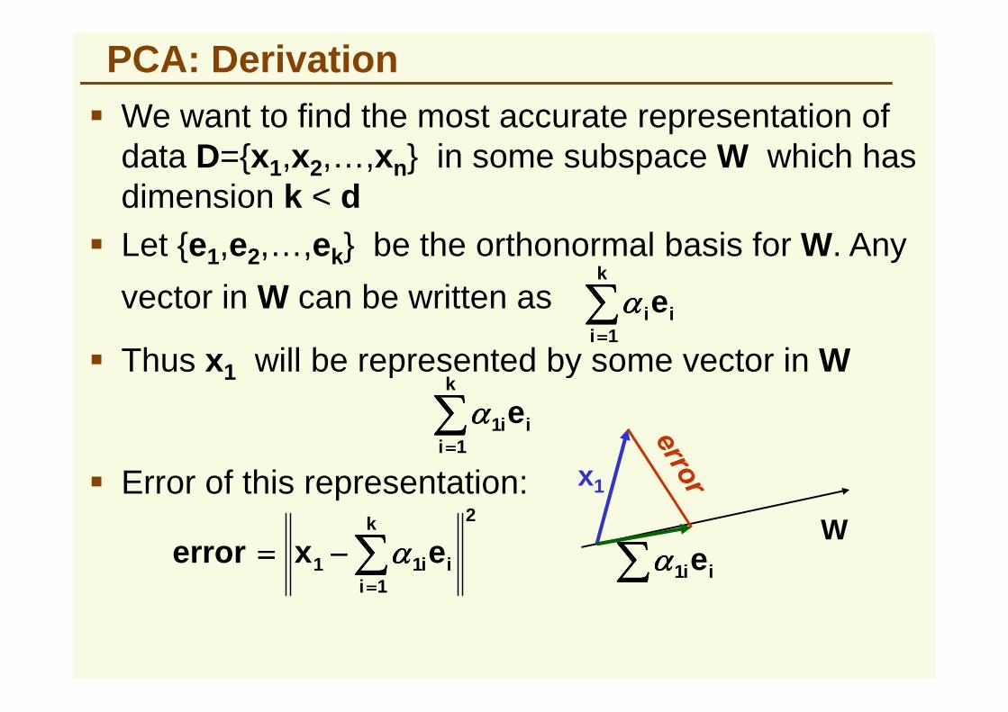
PCA: Derivation� We want to find the most accurate representation of

data D={x1,x2,…,xn} in some subspace W which has dimension k < d

� Let {e1,e2,…,ek} be the orthonormal basis for W. Any

vector in W can be written as ∑∑∑∑====

k

iiie

1

αααα

� Thus x will be represented by some vector in W� Thus x1 will be represented by some vector in W

∑∑∑∑====

k

iiie

11αααα

� Error of this representation:2

111 ∑∑∑∑

====

−−−−====k

iiiexerror αααα

W

x1

∑∑∑∑ iie1αααα

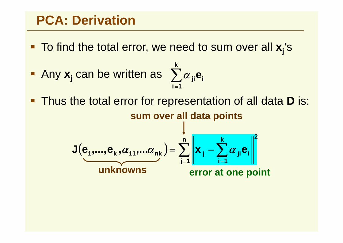
PCA: Derivation

� Any xj can be written as ∑∑∑∑====

k

iijie

1

αααα

� To find the total error, we need to sum over all xj’s

� Thus the total error for representation of all data D is:sum over all data points

error at one point

(((( )))) ∑∑∑∑ ∑∑∑∑==== ====

−−−−====n

j

k

iijijnkk exeeJ

1

2

1111 ,...,,..., αααααααααααα

unknowns

PCA: Derivation

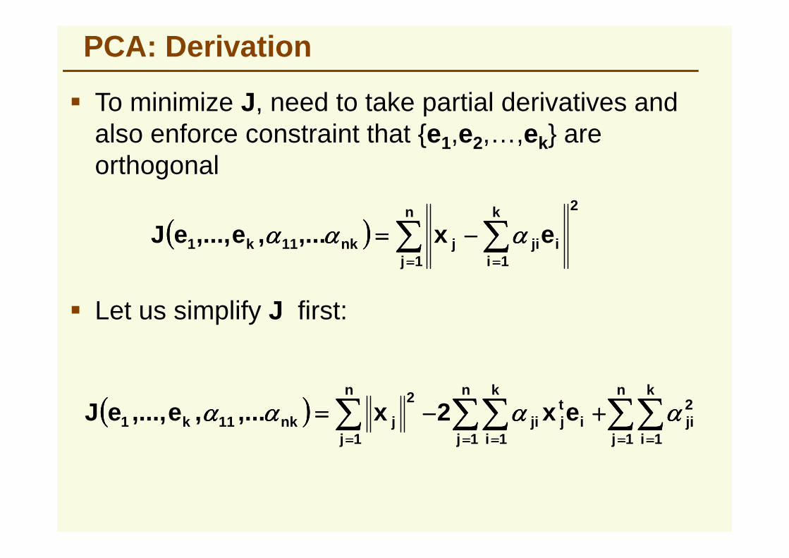
� To minimize J, need to take partial derivatives and also enforce constraint that {e1,e2,…,ek} are orthogonal

(((( )))) ∑∑∑∑ ∑∑∑∑==== ====

−−−−====n

j

k

iijijnkk exeeJ

1

2

1111 ,...,,..., αααααααααααα

� Let us simplify J first:

(((( )))) ∑∑∑∑∑∑∑∑∑∑∑∑∑∑∑∑∑∑∑∑==== ======== ========

++++−−−−====n

1j

k

1i

2ji

n

1j

k

1ii

tjji

n

1j

2

jnk11k1 ex2x,...,e,...,eJ αααααααααααααααα

PCA: Derivation

(((( )))) ∑∑∑∑∑∑∑∑∑∑∑∑∑∑∑∑∑∑∑∑==== ======== ========

++++−−−−====n

1j

k

1i

2ji

n

1j

k

1ii

tjji

n

1j

2


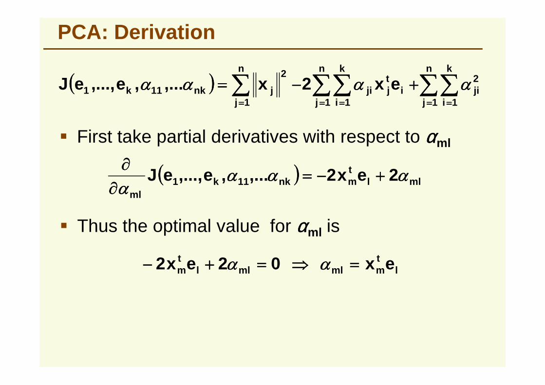
� First take partial derivatives with respect to ααααml

(((( )))) mlltmnkk

ml

exeeJ αααααααααααααααα

22,...,,..., 111 ++++−−−−====∂∂∂∂∂∂∂∂

mlαααα∂∂∂∂

� Thus the optimal value for ααααml is

ltmmlmll

tm exex ====⇒⇒⇒⇒====++++−−−− αααααααα 022

PCA: Derivation

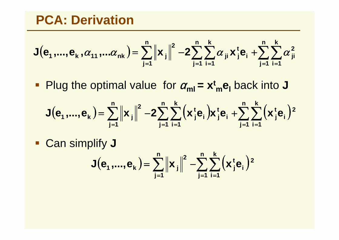
� Plug the optimal value for ααααml = xtmel back into J

(((( )))) (((( )))) (((( ))))∑∑∑∑∑∑∑∑∑∑∑∑∑∑∑∑∑∑∑∑ ++++−−−−====n k

2i

tj

n k

itji

tj

n 2

jk1 exexex2xe,...,eJ

(((( )))) ∑∑∑∑∑∑∑∑∑∑∑∑∑∑∑∑∑∑∑∑==== ======== ========

++++−−−−====n

1j

k

1i

2ji

n

1j

k

1ii

tjji

n

1j

2


∑∑∑∑∑∑∑∑∑∑∑∑∑∑∑∑∑∑∑∑==== ======== ======== 1j 1i

ij1j 1i

ijij1j

jk1

� Can simplify J

(((( )))) (((( ))))∑∑∑∑∑∑∑∑∑∑∑∑==== ========

−−−−====n

1j

k

1i

2i

tj

n

1j

2

jk1 exxe,...,eJ

PCA: Derivation

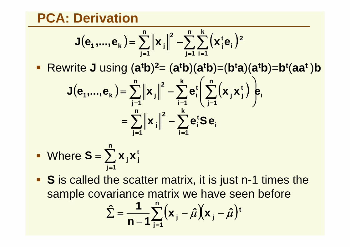
� Rewrite J using (atb)2= (atb)(atb)=(bta)(atb)=bt(aat )b

(((( )))) (((( )))) i

n

j

k

i

n

j

tjj

tijk exxexeeJ ∑∑∑∑ ∑∑∑∑ ∑∑∑∑

==== ==== ====

−−−−====

1 1 1

2

1,...,

∑∑∑∑ ∑∑∑∑−−−−====n k

itij eSex

2

(((( )))) (((( ))))∑∑∑∑∑∑∑∑∑∑∑∑==== ========

−−−−====n

1j

k

1i

2i

tj

n

1j

2

jk1 exxe,...,eJ

∑∑∑∑ ∑∑∑∑==== ====

−−−−====j i

iij eSex1 1

� Where ∑∑∑∑====

====n

j

tjj xxS

1

� S is called the scatter matrix, it is just n-1 times the sample covariance matrix we have seen before

(((( ))))(((( ))))∑∑∑∑====

−−−−−−−−−−−−

====∑∑∑∑n

j

tjj xx

n 1

ˆˆ1

1ˆ µµµµµµµµ

PCA: Derivation

� We should also enforce constraints eitei = 1 for all i

(((( )))) ∑∑∑∑ ∑∑∑∑==== ====

−−−−====n

j

k

ii

tijk eSexeeJ

1 1

2

1,...,

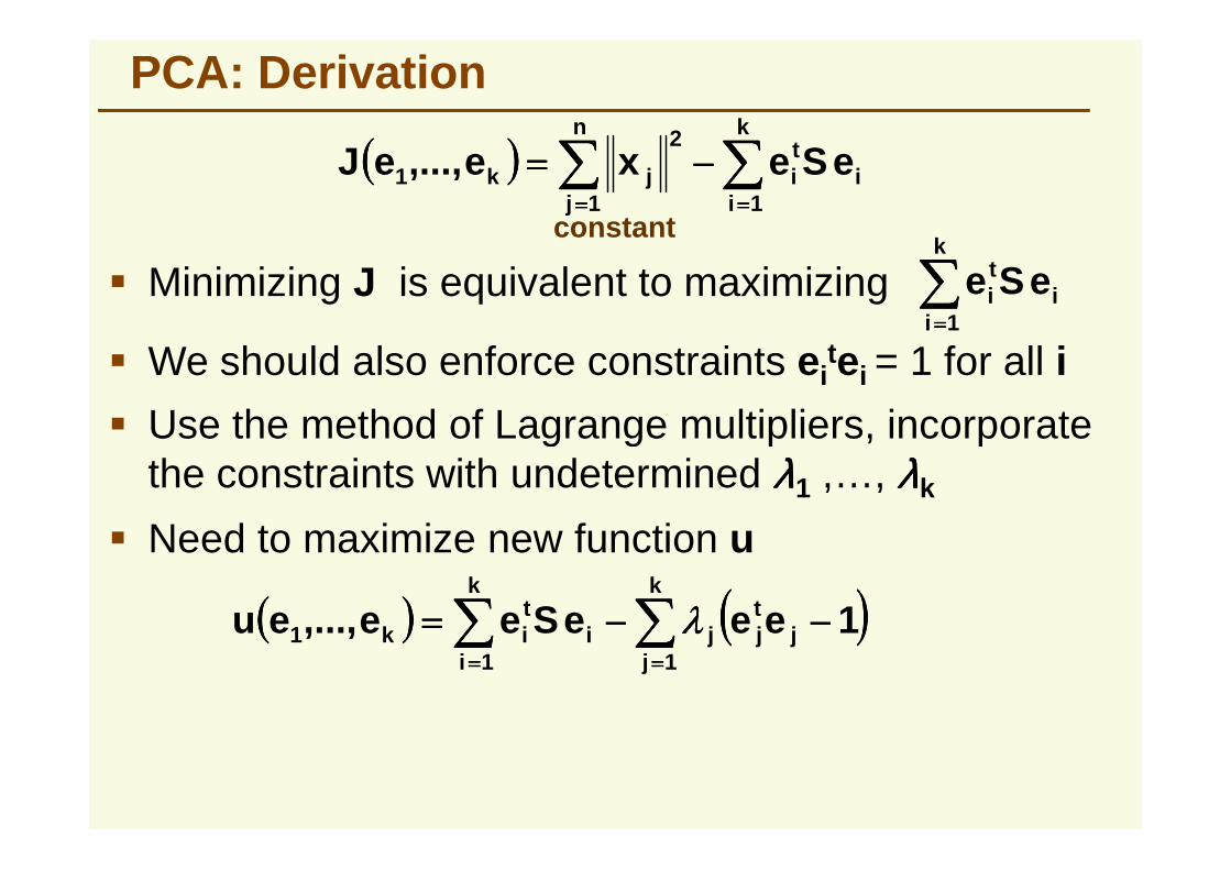
� Use the method of Lagrange multipliers, incorporate

� Minimizing J is equivalent to maximizing ∑∑∑∑====

k

ii

ti eSe

1

constant

� Use the method of Lagrange multipliers, incorporate the constraints with undetermined λλλλ1 ,…, λλλλk

� Need to maximize new function u

(((( )))) (((( ))))∑∑∑∑∑∑∑∑========

−−−−−−−−====k

jj

tjj

k

ii

tik eeeSeeeu

111 1,..., λλλλ

PCA: Derivation

(((( )))) (((( ))))∑∑∑∑∑∑∑∑========

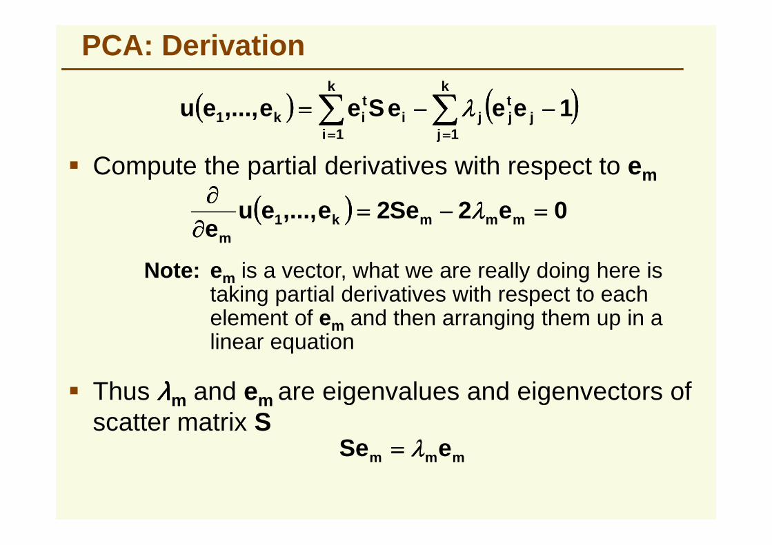
−−−−−−−−====k

jj

tjj

k

ii

tik eeeSeeeu

111 1,..., λλλλ

� Compute the partial derivatives with respect to em

(((( )))) 022,...,1 ====−−−−====∂∂∂∂∂∂∂∂

mmmkm

eSeeeue

λλλλ

Note: em is a vector, what we are really doing here is

� Thus λλλλm and em are eigenvalues and eigenvectors of scatter matrix S

mmm eSe λλλλ====

Note: em is a vector, what we are really doing here is taking partial derivatives with respect to each element of em and then arranging them up in a linear equation

PCA: Derivation

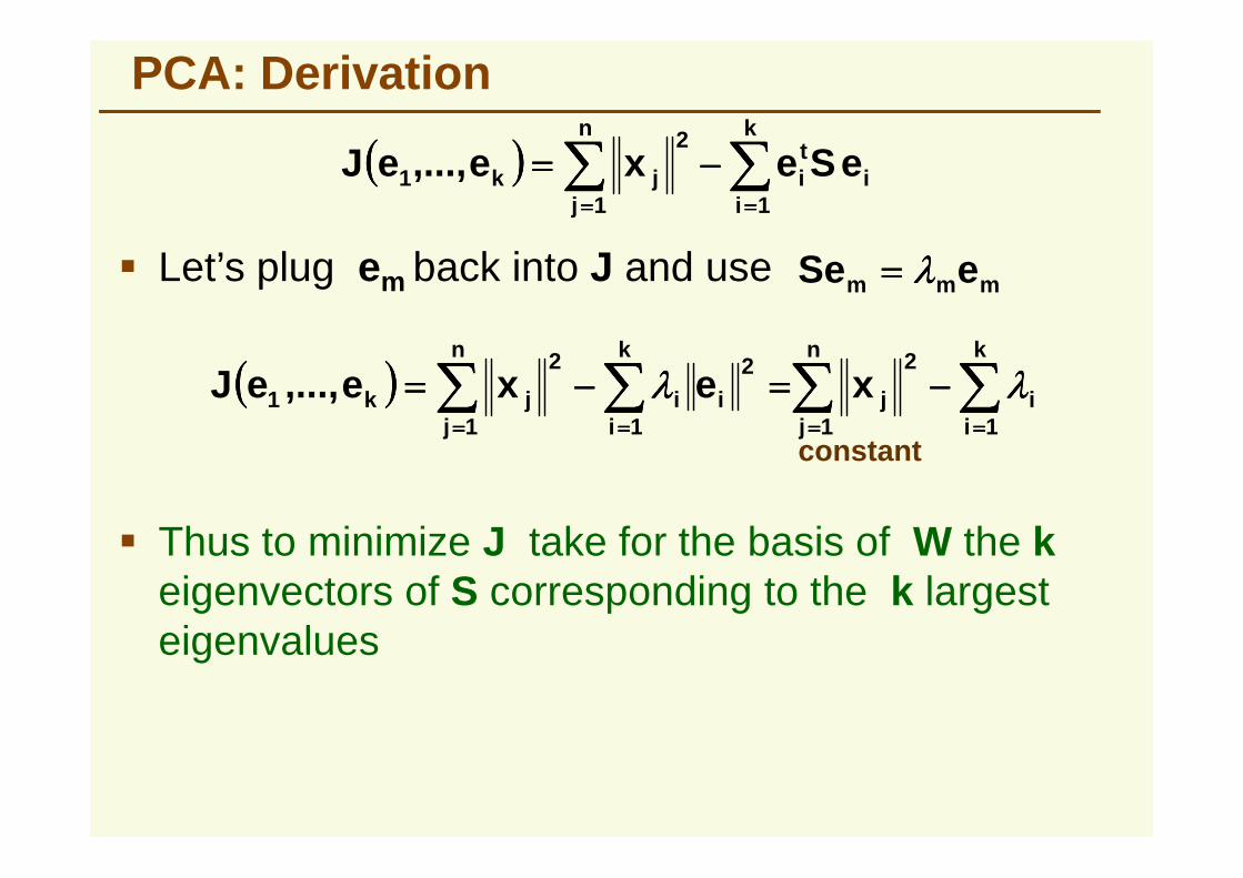
� Let’s plug em back into J and use mmm eSe λλλλ====

(((( )))) ∑∑∑∑ ∑∑∑∑==== ====

−−−−====n

j

k

ii

tijk eSexeeJ

1 1

2

1,...,

(((( )))) ∑∑∑∑ ∑∑∑∑∑∑∑∑ ∑∑∑∑==== ======== ====

−−−−====−−−−====n

1j

k

1ii

2

j

n

1j

k

1i

2ii

2

jk1 xexe,...,eJ λλλλλλλλ

constant==== ======== ==== 1j 1i1j 1i

constant

� Thus to minimize J take for the basis of W the keigenvectors of S corresponding to the k largest eigenvalues

PCA

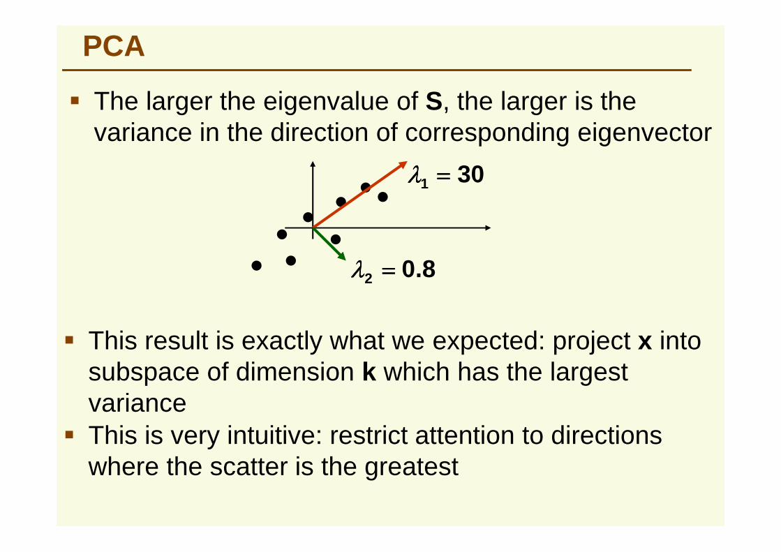
� The larger the eigenvalue of S, the larger is the variance in the direction of corresponding eigenvector

301 ====λλλλ

8.02 ====λλλλ

� This result is exactly what we expected: project x into subspace of dimension k which has the largest variance

� This is very intuitive: restrict attention to directions where the scatter is the greatest

8.02 ====λλλλ

PCA

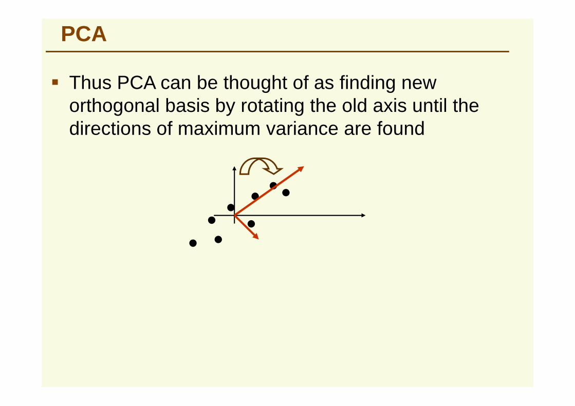
� Thus PCA can be thought of as finding new orthogonal basis by rotating the old axis until the directions of maximum variance are found

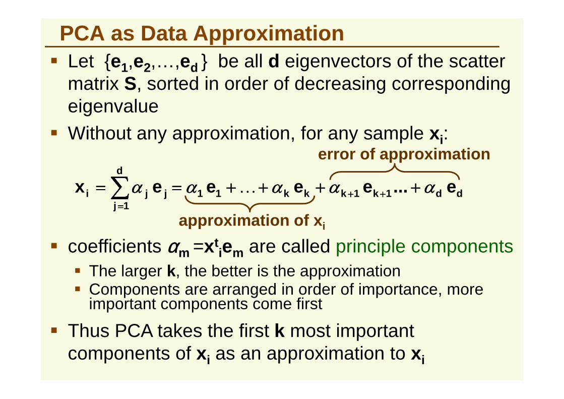
PCA as Data Approximation� Let {e1,e2,…,ed } be all d eigenvectors of the scatter

matrix S, sorted in order of decreasing corresponding eigenvalue

� Without any approximation, for any sample xi:

dd1k1kkk11

d

jji e...eeeex αααααααααααααααααααα ++++++++++++++++======== ++++++++====∑∑∑∑ K

error of approximation

1j====∑∑∑∑

approximation of xi

� coefficients ααααm =xtiem are called principle components

� The larger k, the better is the approximation� Components are arranged in order of importance, more

important components come first

� Thus PCA takes the first k most important components of xi as an approximation to xi

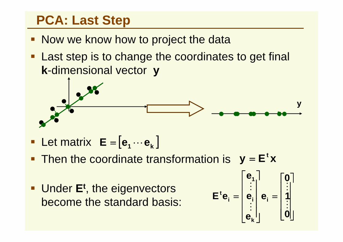
PCA: Last Step� Now we know how to project the data

y

� Last step is to change the coordinates to get final k-dimensional vector y

� Let matrix [[[[ ]]]]keeE L1====

� Then the coordinate transformation is xEy t====

� Under Et, the eigenvectors become the standard basis:

====

====

0

1

01

M

M

M

M

i

k

iit e

e

e

e

eE

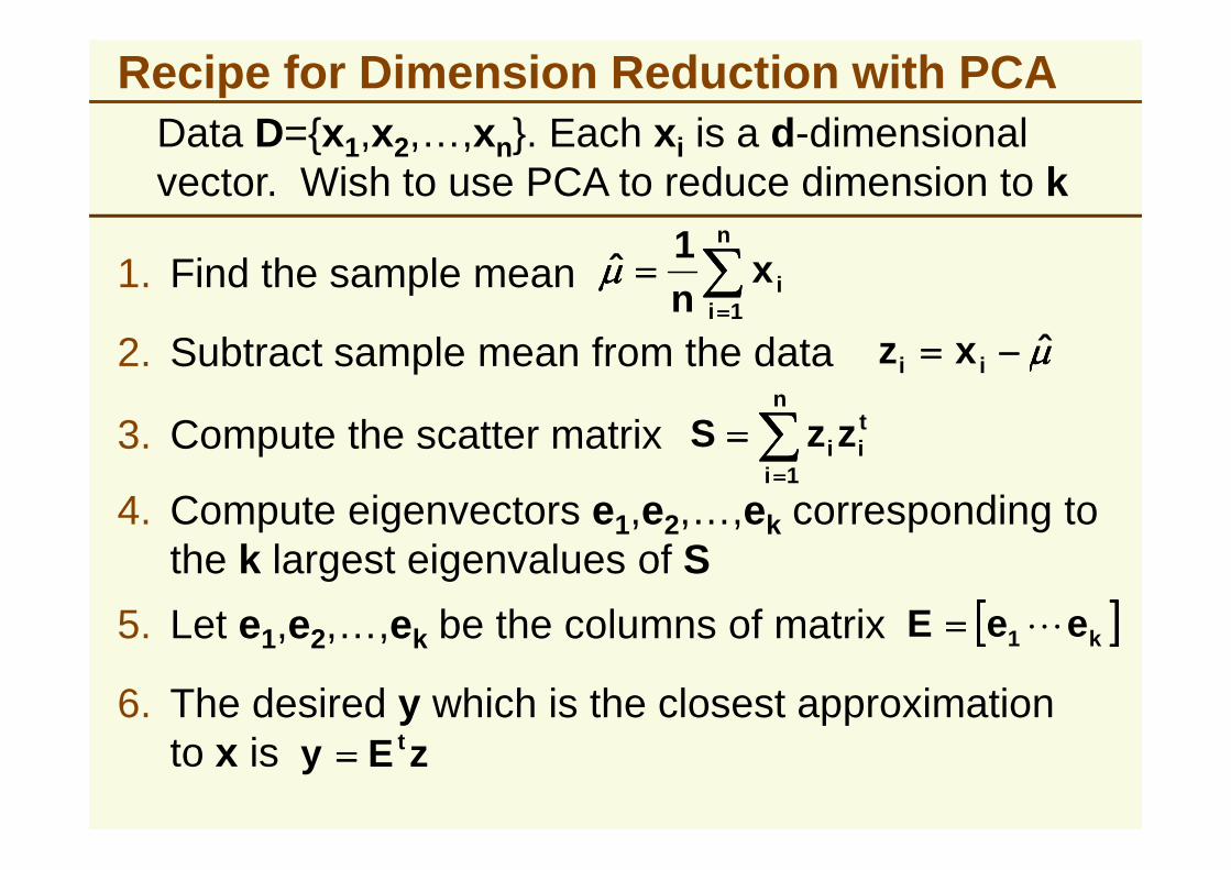
Recipe for Dimension Reduction with PCAData D={x1,x2,…,xn}. Each xi is a d-dimensional vector. Wish to use PCA to reduce dimension to k

1. Find the sample mean ∑∑∑∑====

====n

iix

n 1

1µ̂µµµ

2. Subtract sample mean from the data µµµµ̂−−−−==== ii xz

3. Compute the scatter matrix ∑∑∑∑====n

tzzS3. Compute the scatter matrix ∑∑∑∑====

====i

iizzS1

4. Compute eigenvectors e1,e2,…,ek corresponding to the k largest eigenvalues of S

5. Let e1,e2,…,ek be the columns of matrix [[[[ ]]]]keeE L1====

6. The desired y which is the closest approximation to x is zEy t====

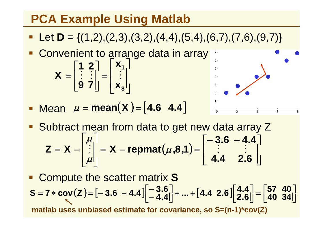
PCA Example Using Matlab� Let D = {(1,2),(2,3),(3,2),(4,4),(5,4),(6,7),(7,6),(9,7)}

� Convenient to arrange data in array

====

====

8

1

x

x

79

21X MMM

� Mean (((( )))) [[[[ ]]]]4.46.4Xmean ========µµµµ� Mean

� Subtract mean from data to get new data array Z

(((( ))))

−−−−−−−−====−−−−====

−−−−====

6.24.4

4.46.31,8,repmatXXZ MMM µµµµ

µµµµ

µµµµ

� Compute the scatter matrix S(((( )))) [[[[ ]]]] [[[[ ]]]]

====

++++++++

−−−−−−−−−−−−−−−−====∗∗∗∗==== 3440

40576.24.46.24.4...4.4

6.34.46.3Zcov7S

matlab uses unbiased estimate for covariance, so S=(n-1)*cov(Z)

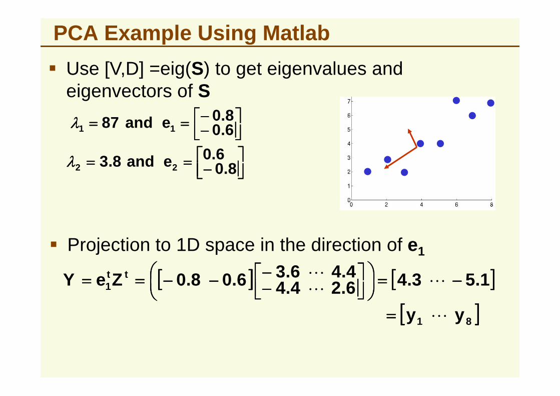
PCA Example Using Matlab

� Use [V,D] =eig(S) to get eigenvalues and eigenvectors of S

−−−−−−−−======== 6.0

8.0eand87 11λλλλ

−−−−======== 8.0

6.0eand8.3 22λλλλ

� Projection to 1D space in the direction of e1

[[[[ ]]]] [[[[ ]]]]1.53.46.24.44.46.36.08.0ZeY tt

1 −−−−====

−−−−−−−−−−−−−−−−======== L

LL

[[[[ ]]]]81 yy L====

Curse of Dimensionality, Dimensionality Reduction with …rita/uml_course/add_mat/PCA.pdf · Curse...

Documents

Transcript of Curse of Dimensionality, Dimensionality Reduction with …rita/uml_course/add_mat/PCA.pdf · Curse...