Curl and Divergence - NDSU - North Dakota State …micohen/oldlecturenotes...Curl and Divergence,...
36
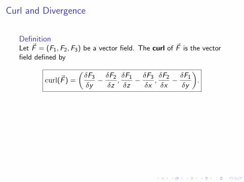
Curl and Divergence Definition Let ~ F =(F 1 , F 2 , F 3 ) be a vector field. The curl of ~ F is the vector field defined by curl( ~ F )= δF 3 δy - δF 2 δz , δF 1 δz - δF 3 δx , δF 2 δx - δF 1 δy .
Transcript of Curl and Divergence - NDSU - North Dakota State …micohen/oldlecturenotes...Curl and Divergence,...
Curl and Divergence
DefinitionLet ~F = (F1,F2,F3) be a vector field. The curl of ~F is the vectorfield defined by
curl(~F ) =
(δF3
δy− δF2
δz,δF1
δz− δF3
δx,δF2
δx− δF1
δy
).
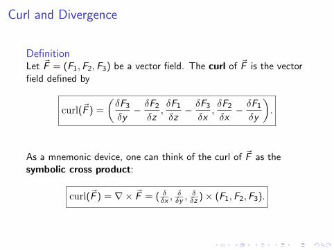
As a mnemonic device, one can think of the curl of ~F as thesymbolic cross product:
curl(~F ) = ∇× ~F = ( δδx ,
δδy ,
δδz )× (F1,F2,F3).
Curl and Divergence
DefinitionLet ~F = (F1,F2,F3) be a vector field. The curl of ~F is the vectorfield defined by
curl(~F ) =
(δF3
δy− δF2
δz,δF1
δz− δF3
δx,δF2
δx− δF1
δy
).
As a mnemonic device, one can think of the curl of ~F as thesymbolic cross product:
curl(~F ) = ∇× ~F = ( δδx ,
δδy ,
δδz )× (F1,F2,F3).
Curl and Divergence, contd.
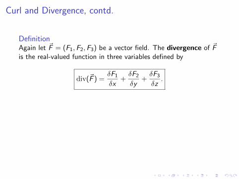
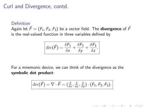
DefinitionAgain let ~F = (F1,F2,F3) be a vector field. The divergence of ~Fis the real-valued function in three variables defined by
div(~F ) =δF1
δx+δF2
δy+δF3
δz.
For a mnemonic device, we can think of the divergence as thesymbolic dot product:
div(~F ) = ∇ · ~F = ( δδx ,
δδy ,
δδz ) · (F1,F2,F3).
Curl and Divergence, contd.
DefinitionAgain let ~F = (F1,F2,F3) be a vector field. The divergence of ~Fis the real-valued function in three variables defined by
div(~F ) =δF1
δx+δF2
δy+δF3
δz.
For a mnemonic device, we can think of the divergence as thesymbolic dot product:
div(~F ) = ∇ · ~F = ( δδx ,
δδy ,
δδz ) · (F1,F2,F3).
Physical Significance
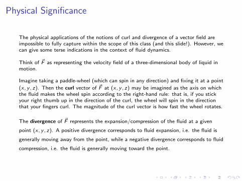
The physical applications of the notions of curl and divergence of a vector field areimpossible to fully capture within the scope of this class (and this slide!). However, wecan give some terse indications in the context of fluid dynamics.
Think of ~F as representing the velocity field of a three-dimensional body of liquid inmotion.
Imagine taking a paddle-wheel (which can spin in any direction) and fixing it at a point
(x , y , z). Then the curl vector of ~F at (x , y , z) may be imagined as the axis on whichthe fluid makes the wheel spin according to the right-hand rule: that is, if you stickyour right thumb up in the direction of the curl, the wheel will spin in the directionthat your fingers curl. The magnitude of the curl vector is how fast the wheel rotates.
The divergence of ~F represents the expansion/compression of the fluid at a given
point (x , y , z). A positive divergence corresponds to fluid expansion, i.e. the fluid is
generally moving away from the point, while a negative divergence corresponds to fluid
compression, i.e. the fluid is generally moving toward the point.
Physical Significance
The physical applications of the notions of curl and divergence of a vector field areimpossible to fully capture within the scope of this class (and this slide!). However, wecan give some terse indications in the context of fluid dynamics.
Think of ~F as representing the velocity field of a three-dimensional body of liquid inmotion.
Imagine taking a paddle-wheel (which can spin in any direction) and fixing it at a point
(x , y , z). Then the curl vector of ~F at (x , y , z) may be imagined as the axis on whichthe fluid makes the wheel spin according to the right-hand rule: that is, if you stickyour right thumb up in the direction of the curl, the wheel will spin in the directionthat your fingers curl. The magnitude of the curl vector is how fast the wheel rotates.
The divergence of ~F represents the expansion/compression of the fluid at a given
point (x , y , z). A positive divergence corresponds to fluid expansion, i.e. the fluid is
generally moving away from the point, while a negative divergence corresponds to fluid
compression, i.e. the fluid is generally moving toward the point.
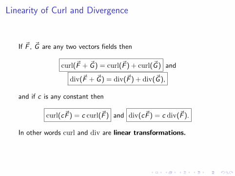
Linearity of Curl and Divergence
If ~F , ~G are any two vectors fields then
curl(~F + ~G ) = curl(~F ) + curl(~G ) and
div(~F + ~G ) = div(~F ) + div(~G ),
and if c is any constant then
curl(c~F ) = c curl(~F ) and div(c~F ) = c div(~F ).
In other words curl and div are linear transformations.
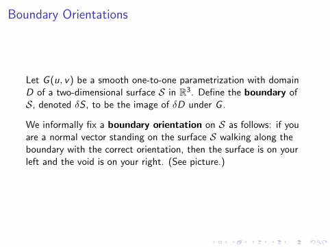
Boundary Orientations
Let G (u, v) be a smooth one-to-one parametrization with domainD of a two-dimensional surface S in R3. Define the boundary ofS, denoted δS , to be the image of δD under G .
We informally fix a boundary orientation on S as follows: if youare a normal vector standing on the surface S walking along theboundary with the correct orientation, then the surface is on yourleft and the void is on your right. (See picture.)
Stokes’ Theorem
Theorem (Stokes’ Theorem)
Let S be a surface parametrized by a smooth one-to-one functionG (u, v) with domain D, where δD is comprised of simple closedcurves. Then ∮
δS~F · ds =
∫ ∫Scurl(~F ) · dS.
Example
Verify Stokes’ theorem for the field ~F = (−y , 2x , x + z) and theupper unit hemisphere S, with outward-pointing normal vectors.
SolutionKnown: ~F = (−y , 2x , x + z)
First we will just compute the line integral about the boundary δS , which is the unitcircle in the xy -plane oriented counterclockwise. We can parametrize δS in the usualway:
~c(t) = (cos t, sin t, 0) on the domain [0, 2π].
Now compute:
∮δS~F · ds =
∫ 2π
0
~F (~c(t)) · ~c ′(t)dt
=
∫ 2π
0(− sin t, 2 cos t, cos t) · (− sin t, cos t, 0)dt
=
∫ 2π
0(sin2 t + 2 cos2 t)dt
=
∫ 2π
0(1 + cos2 t)dt
=
∫ 2π
0
(3
2+
1
2cos 2t
)dt
=
[3
2t +
1
4sin 2t
]2π
0
= 3π.
Solution, contd.
Known: ~F = (−y , 2x , x + z)∮δS~F · ds = 3π
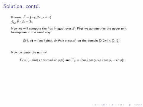
Now we will compute the flux integral over S. First we parametrize the upper unithemisphere in the usual way:
G(θ, φ) = (cos θ sinφ, sin θ sinφ, cosφ) on the domain [0, 2π]× [0, π2
].
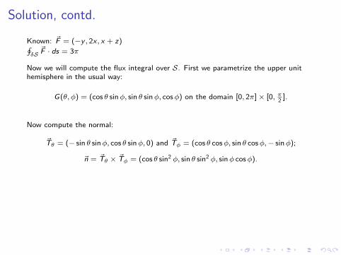
Now compute the normal:
~Tθ = (− sin θ sinφ, cos θ sinφ, 0) and ~Tφ = (cos θ cosφ, sin θ cosφ,− sinφ);
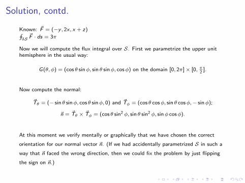
~n = ~Tθ × ~Tφ = (cos θ sin2 φ, sin θ sin2 φ, sinφ cosφ).
At this moment we verify mentally or graphically that we have chosen the correct
orientation for our normal vector ~n. (If we had accidentally parametrized S in such a
way that ~n faced the wrong direction, then we could fix the problem by just flipping
the sign on ~n.)
Solution, contd.
Known: ~F = (−y , 2x , x + z)∮δS~F · ds = 3π
Now we will compute the flux integral over S. First we parametrize the upper unithemisphere in the usual way:
G(θ, φ) = (cos θ sinφ, sin θ sinφ, cosφ) on the domain [0, 2π]× [0, π2
].
Now compute the normal:
~Tθ = (− sin θ sinφ, cos θ sinφ, 0) and ~Tφ = (cos θ cosφ, sin θ cosφ,− sinφ);
~n = ~Tθ × ~Tφ = (cos θ sin2 φ, sin θ sin2 φ, sinφ cosφ).
At this moment we verify mentally or graphically that we have chosen the correct
orientation for our normal vector ~n. (If we had accidentally parametrized S in such a
way that ~n faced the wrong direction, then we could fix the problem by just flipping
the sign on ~n.)
Solution, contd.
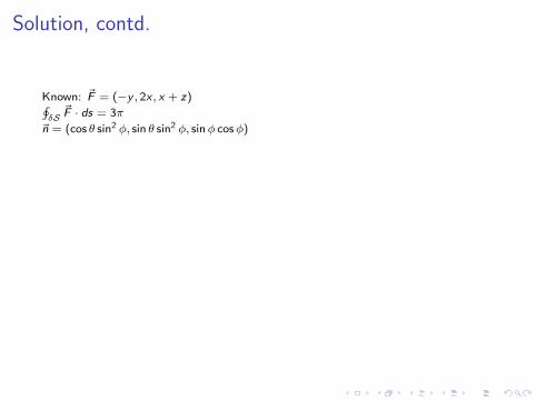
Known: ~F = (−y , 2x , x + z)∮δS~F · ds = 3π
~n = (cos θ sin2 φ, sin θ sin2 φ, sinφ cosφ)
Next compute curl(~F ):
curl(~F ) = det
~i ~j ~kδδx
δδy
δδz
−y 2x x + z
=
(δ
δy(x + z)−
δ
δz(2x),−
δ
δx(x + z) +
δ
δz(−y),
δ
δx(2x)−
δ
δy(−y)
)= (0,−1, 3).
Solution, contd.
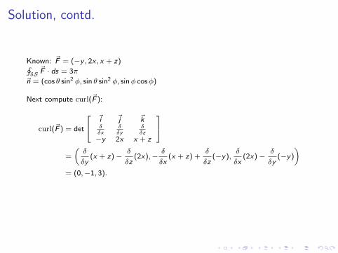
Known: ~F = (−y , 2x , x + z)∮δS~F · ds = 3π
~n = (cos θ sin2 φ, sin θ sin2 φ, sinφ cosφ)
Next compute curl(~F ):
curl(~F ) = det
~i ~j ~kδδx
δδy
δδz
−y 2x x + z
=
(δ
δy(x + z)−
δ
δz(2x),−
δ
δx(x + z) +
δ
δz(−y),
δ
δx(2x)−
δ
δy(−y)
)= (0,−1, 3).
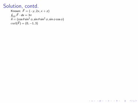
Solution, contd.Known: ~F = (−y , 2x , x + z)∮δS~F · ds = 3π
~n = (cos θ sin2 φ, sin θ sin2 φ, sinφ cosφ)
curl(~F ) = (0,−1, 3)
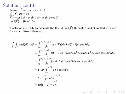
Finally we are ready to compute the flux of curl(~F ) through S and show that it equals3π as per Stokes’ theorem.
∫ ∫Scurl(~F ) · dS =
∫ π/2
0
∫ 2π
0curl(~F )(G(θ, φ)) · ~n(θ, φ)dθdφ
=
∫ π/2
0
∫ 2π
0(0,−1, 3) · (cos θ sin2 φ, sin θ sin2 φ, sinφ cosφ)dθdφ
=
∫ π/2
0
∫ 2π
0(− sin θ sin2 φ+ 3 sinφ cosφ)dθdφ
= 3 · 2π∫ π/2
0sinφ cosφdφ
= 6π ·[
1
2sin2 φ
]π/2
0
= 3π[1− 0] = 3π.
Solution, contd.Known: ~F = (−y , 2x , x + z)∮δS~F · ds = 3π
~n = (cos θ sin2 φ, sin θ sin2 φ, sinφ cosφ)
curl(~F ) = (0,−1, 3)
Finally we are ready to compute the flux of curl(~F ) through S and show that it equals3π as per Stokes’ theorem.
∫ ∫Scurl(~F ) · dS =
∫ π/2
0
∫ 2π
0curl(~F )(G(θ, φ)) · ~n(θ, φ)dθdφ
=
∫ π/2
0
∫ 2π
0(0,−1, 3) · (cos θ sin2 φ, sin θ sin2 φ, sinφ cosφ)dθdφ
=
∫ π/2
0
∫ 2π
0(− sin θ sin2 φ+ 3 sinφ cosφ)dθdφ
= 3 · 2π∫ π/2
0sinφ cosφdφ
= 6π ·[
1
2sin2 φ
]π/2
0
= 3π[1− 0] = 3π.
Higher-Dimensional Boundary Orientations
Now let W denote a closed bounded region in R3 enclosed by asmooth parametrized surface S = δW, the boundary of W.
We orient δW by requiring that the normal vectors ~n pointoutward, away from W.
Divergence Theorem
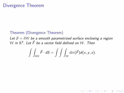
Theorem (Divergence Theorem)
Let S = δW be a smooth parametrized surface enclosing a regionW in R3. Let ~F be a vector field defined on W. Then∫ ∫
δW~F · dS =
∫ ∫ ∫W
div(~F )d(x , y , z).
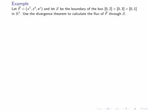
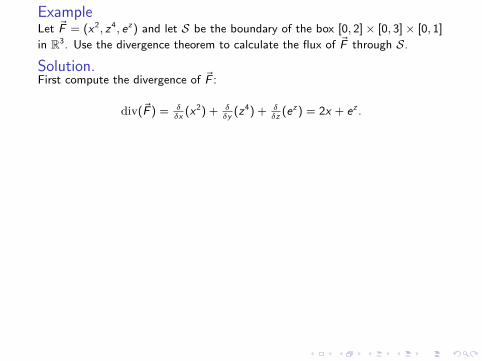
ExampleLet ~F = (x2, z4, ez) and let S be the boundary of the box [0, 2]× [0, 3]× [0, 1]
in R3. Use the divergence theorem to calculate the flux of ~F through S.
Solution.First compute the divergence of ~F :
div(~F ) = δδx
(x2) + δδy
(z4) + δδz
(ez) = 2x + ez .
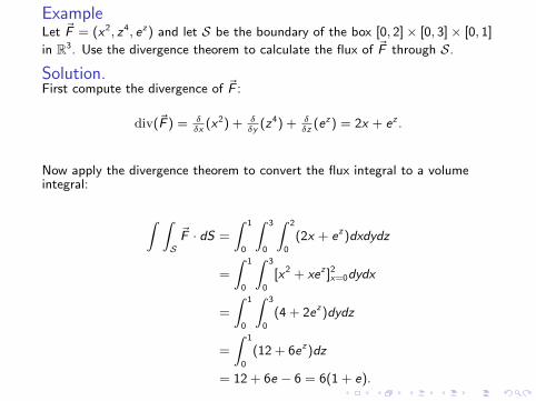
Now apply the divergence theorem to convert the flux integral to a volumeintegral:
∫ ∫S
~F · dS =
∫ 1
0
∫ 3
0
∫ 2
0
(2x + ez)dxdydz
=
∫ 1
0
∫ 3
0
[x2 + xez ]2x=0dydx
=
∫ 1
0
∫ 3
0
(4 + 2ez)dydz
=
∫ 1
0
(12 + 6ez)dz
= 12 + 6e − 6 = 6(1 + e).
ExampleLet ~F = (x2, z4, ez) and let S be the boundary of the box [0, 2]× [0, 3]× [0, 1]
in R3. Use the divergence theorem to calculate the flux of ~F through S.
Solution.First compute the divergence of ~F :
div(~F ) = δδx
(x2) + δδy
(z4) + δδz
(ez) = 2x + ez .
Now apply the divergence theorem to convert the flux integral to a volumeintegral:
∫ ∫S
~F · dS =
∫ 1
0
∫ 3
0
∫ 2
0
(2x + ez)dxdydz
=
∫ 1
0
∫ 3
0
[x2 + xez ]2x=0dydx
=
∫ 1
0
∫ 3
0
(4 + 2ez)dydz
=
∫ 1
0
(12 + 6ez)dz
= 12 + 6e − 6 = 6(1 + e).
Consequences of Stokes’ and Divergence Theorems
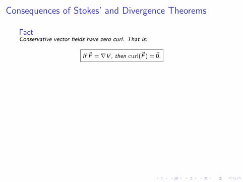
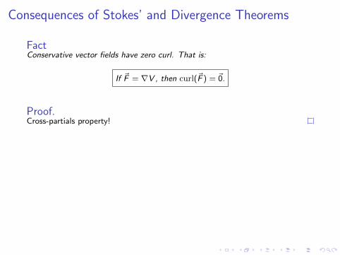
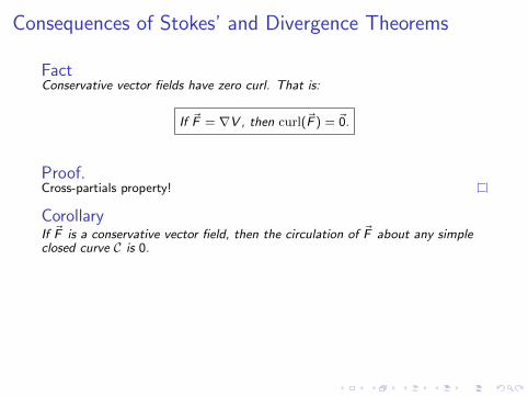
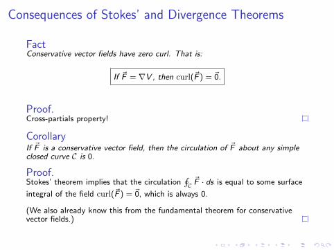
FactConservative vector fields have zero curl. That is:
If ~F = ∇V , then curl(~F ) = ~0.
Proof.Cross-partials property!
CorollaryIf ~F is a conservative vector field, then the circulation of ~F about any simpleclosed curve C is 0.
Proof.Stokes’ theorem implies that the circulation
∮C~F · ds is equal to some surface
integral of the field curl(~F ) = ~0, which is always 0.
(We also already know this from the fundamental theorem for conservativevector fields.)
Consequences of Stokes’ and Divergence Theorems
FactConservative vector fields have zero curl. That is:
If ~F = ∇V , then curl(~F ) = ~0.
Proof.Cross-partials property!
CorollaryIf ~F is a conservative vector field, then the circulation of ~F about any simpleclosed curve C is 0.
Proof.Stokes’ theorem implies that the circulation
∮C~F · ds is equal to some surface
integral of the field curl(~F ) = ~0, which is always 0.
(We also already know this from the fundamental theorem for conservativevector fields.)
Consequences of Stokes’ and Divergence Theorems, contd.
FactCurl fields have zero divergence. That is:
If ~F = curl(~A), then div(~F ) = 0.
Proof.A consequence of Clairaut’s theorem! Remember this theorem says mixedsecond-order partial derivatives are equal for continuously differentiablefunctions. Try working through this on your own.
CorollaryIf ~F is the curl field of some vector field ~A, then the flux of ~F through anyclosed surface is 0.
Proof.The divergence theorem says that the flux of ~F is equal to a volume integral of
the function div(~F ), again a 0 function which gives a 0 integral.
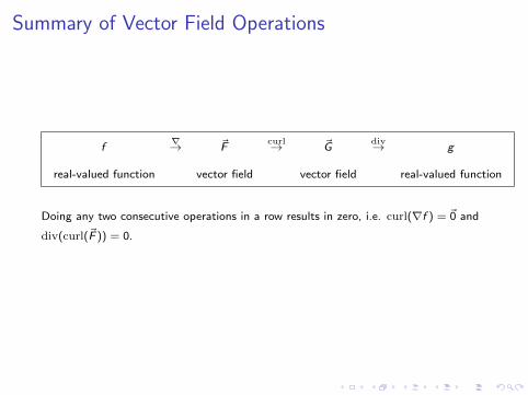
Summary of Vector Field Operations
f∇→ ~F
curl→ ~Gdiv→ g
real-valued function vector field vector field real-valued function
Doing any two consecutive operations in a row results in zero, i.e. curl(∇f ) = ~0 and
div(curl(~F )) = 0.

Thanks
Thanks for a great semester!


![arXiv:2007.02335v1 [math.CA] 5 Jul 2020arXiv:2007.02335v1 [math.CA] 5 Jul 2020 Bilinear Decomposition and Divergence-Curl Estimates on Products Related to Local Hardy Spaces and Their](https://static.fdocument.org/doc/165x107/601581c6fca168615865fb1d/arxiv200702335v1-mathca-5-jul-2020-arxiv200702335v1-mathca-5-jul-2020.jpg)