Convex OptimizationLecture 16

Today:

• Projected Gradient Descent

• Conditional Gradient Descent

• Stochastic Gradient Descent

• Random Coordinate Descent

Recall: Gradient Descent

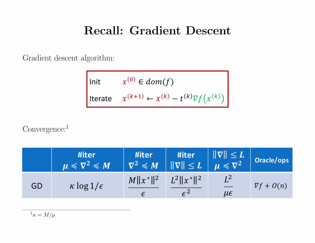
Gradient descent algorithm:

Gradient Descent(Steepest Descent w.r.t Euclidean Norm)

Δ𝑥 = −𝛻𝑓 𝑥 𝑘

Reminder: We are violating here the distinction between the primal space and the dual gradient space—we are implicitly linking them by matching representations w.r.t. a chosen basis

Note: Δ𝑥 is not normalized (i.e. we don’t require Δ𝑥 2 = 1). This just changes the meaning of 𝑡.

How do we choose the stepsize 𝑡 𝑘 ?

Init 𝑥 0 ∈ 𝑑𝑜𝑚(𝑓)

Iterate 𝑥 𝑘+1 ← 𝑥 𝑘 − 𝑡 𝑘 𝛻𝑓 𝑥 𝑘

Convergence:1

Lower'Bounds• Some%upper%bounds:

• Is%this%the%best%we%can%do?• What%if%we%allow%! "# ops?• YES!• When%using%only%first>order%oracle%(gradients)

• History:• Nemirovski&%Yudin (1983)• Nesterov (2004)

#iter$ ≼ &' ≼ (

#iter&' ≼ (

#iter& ≤ *

& ≤ *$ ≼ &' Oracle/ops

GD + log1/1 2 3∗ #

15# 3∗ #

1#5#61 78 + !(")

A>GD + log1/1 2 3∗ #

1x x 78 + !(")1κ =M/µ

Smoothness and Strong Convexity

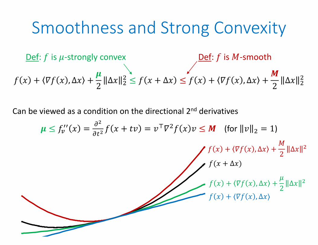
𝑓 𝑥 + 𝛻𝑓 𝑥 , Δ𝑥 +𝝁2

Δ𝑥 ≤ 𝑓 𝑥 + Δ𝑥 ≤ 𝑓 𝑥 + 𝛻𝑓 𝑥 , Δ𝑥 +𝑴2

Δ𝑥

Can be viewed as a condition on the directional 2nd derivatives

𝝁 ≤ 𝑓 𝑥 = 𝑓 𝑥 + 𝑡𝑣 = 𝑣 𝛻 𝑓 𝑥 𝑣 ≤ 𝑴 (for 𝑣 = 1)

Def: 𝑓 is 𝜇-strongly convex Def: 𝑓 is 𝑀-smooth

𝑓(𝑥 + Δ𝑥)

𝑓 𝑥 + ⟨𝛻𝑓 𝑥 , Δ𝑥⟩

𝑓 𝑥 + 𝛻𝑓 𝑥 , Δ𝑥 +𝜇2

Δ𝑥

𝑓 𝑥 + 𝛻𝑓 𝑥 , Δ𝑥 +𝑀2

Δ𝑥

What about constraints?

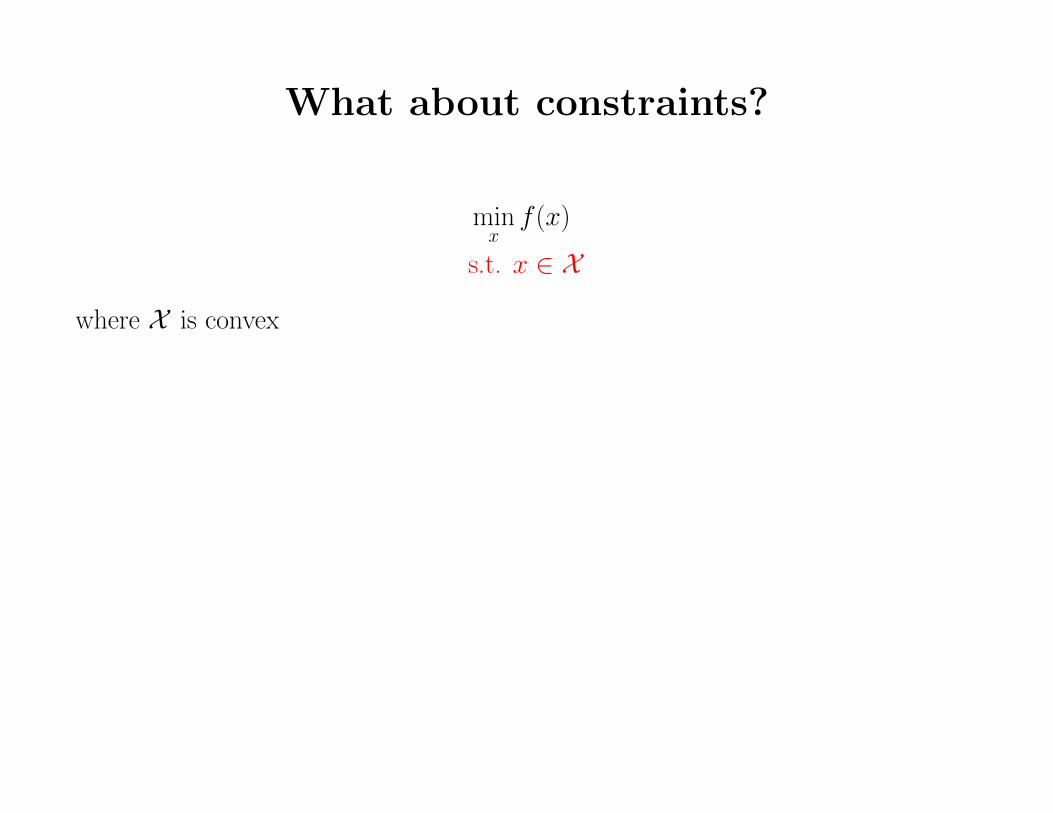
minxf (x)

s.t. x ∈ X

where X is convex

Projected Gradient Descent

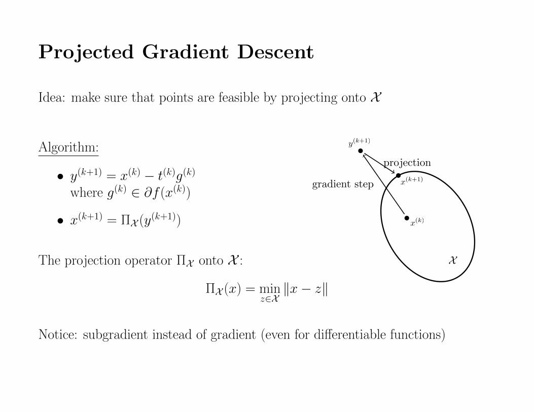
Idea: make sure that points are feasible by projecting onto X

Algorithm:

3.1. Projected Subgradient Descent for Lipschitz functions 21

xt

yt+1

gradient step

(3.2)

xt+1

projection (3.3)

X

Fig. 3.2 Illustration of the Projected Subgradient Descent method.

not exist) by a subgradient g 2 @f(x). Secondly, and more importantly,

we make sure that the updated point lies in X by projecting back (if

necessary) onto it. This gives the Projected Subgradient Descent algo-

rithm which iterates the following equations for t 1:

yt+1 = xt gt, where gt 2 @f(xt), (3.2)

xt+1 = X (yt+1). (3.3)

This procedure is illustrated in Figure 3.2. We prove now a rate of

convergence for this method under the above assumptions.

Theorem 3.1. The Projected Subgradient Descent with = RLp

tsat-

isfies

f

1

t

tX

s=1

xs

! f(x) RLp

t.

Proof. Using the definition of subgradients, the definition of the

method, and the elementary identity 2a>b = kak2 + kbk2 ka bk2,

x(k)

x(k+1)

y(k+1)

• y(k+1) = x(k) − t(k)g(k)where g(k) ∈ ∂f (x(k))

• x(k+1) = ΠX (y(k+1))

The projection operator ΠX onto X :

ΠX (x) = minz∈X‖x− z‖

Notice: subgradient instead of gradient (even for differentiable functions)

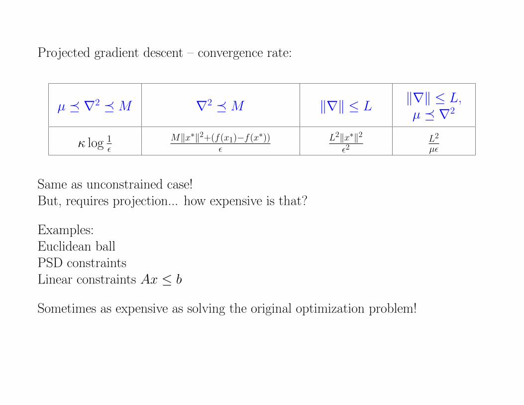
Projected gradient descent – convergence rate:

µ ∇2 M ∇2 M ‖∇‖ ≤ L‖∇‖ ≤ L,µ ∇2

κ log 1ε

M‖x∗‖2+(f(x1)−f(x∗))ε

L2‖x∗‖2ε2

L2

µε

Same as unconstrained case!But, requires projection... how expensive is that?

Examples:Euclidean ballPSD constraintsLinear constraints Ax ≤ b

Sometimes as expensive as solving the original optimization problem!

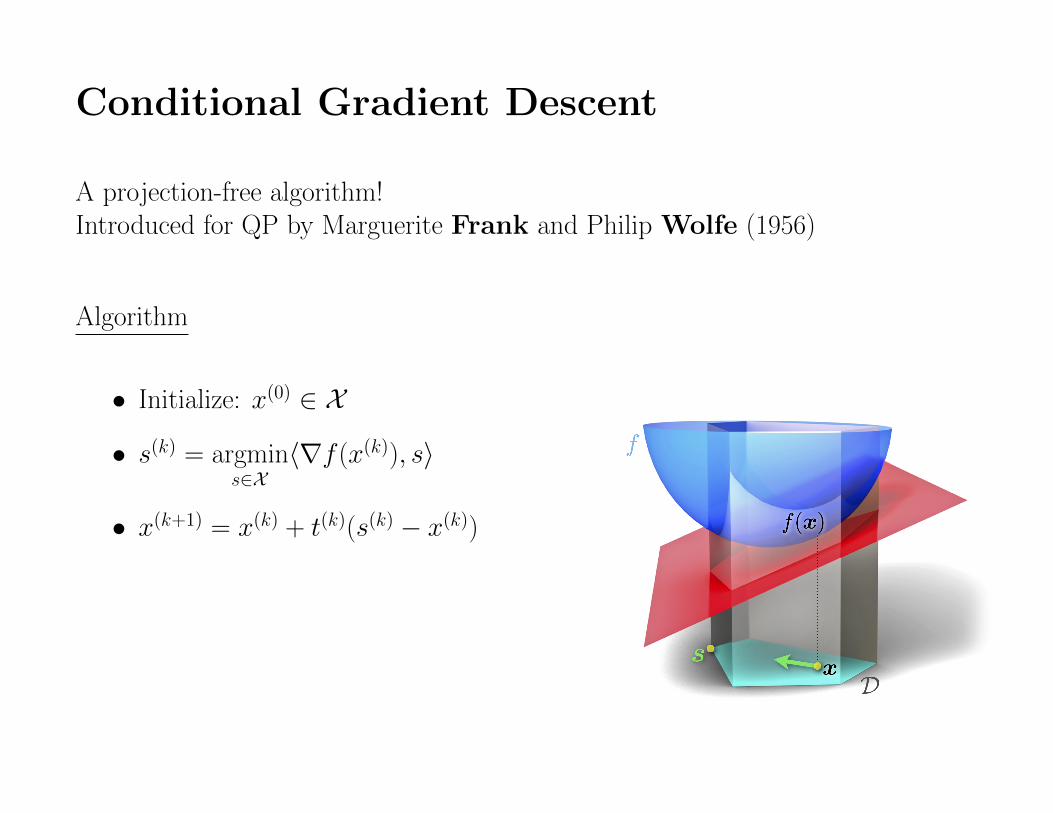
Conditional Gradient Descent

A projection-free algorithm!Introduced for QP by Marguerite Frank and Philip Wolfe (1956)

Algorithm

• Initialize: x(0) ∈ X

• s(k) = argmins∈X

〈∇f (x(k)), s〉

• x(k+1) = x(k) + t(k)(s(k) − x(k))

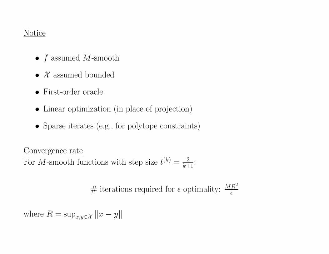
Notice

• f assumed M -smooth

• X assumed bounded

• First-order oracle

• Linear optimization (in place of projection)

• Sparse iterates (e.g., for polytope constraints)

Convergence rate

For M -smooth functions with step size t(k) = 2k+1:

# iterations required for ε-optimality: MR2

ε

where R = supx,y∈X ‖x− y‖

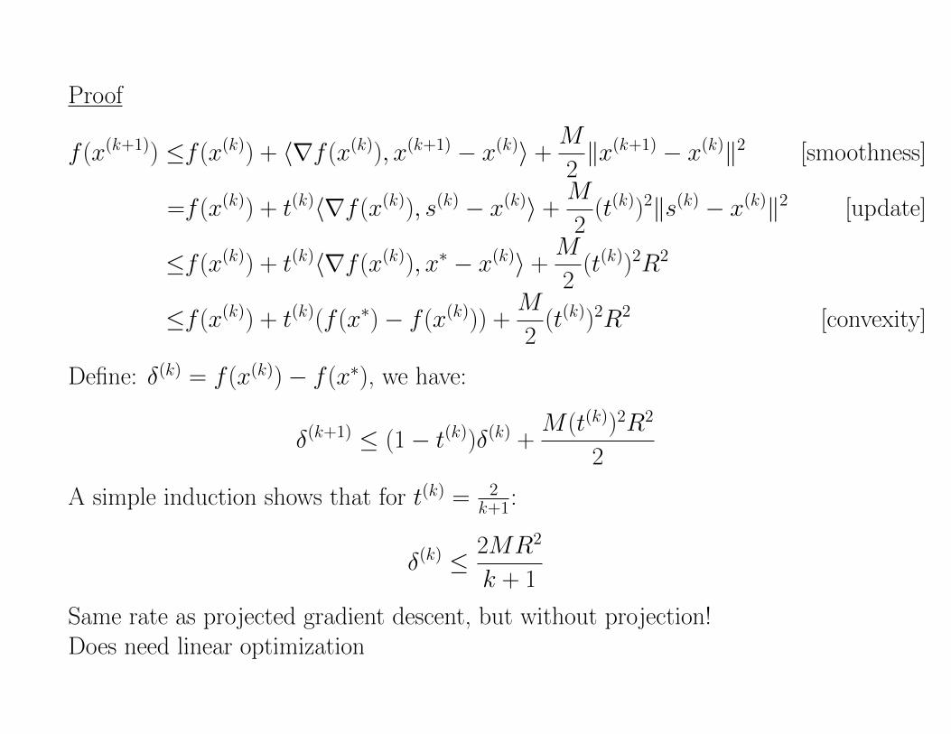
Proof

f (x(k+1)) ≤f (x(k)) + 〈∇f (x(k)), x(k+1) − x(k)〉 +M

2‖x(k+1) − x(k)‖2 [smoothness]

=f (x(k)) + t(k)〈∇f (x(k)), s(k) − x(k)〉 +M

2(t(k))2‖s(k) − x(k)‖2 [update]

≤f (x(k)) + t(k)〈∇f (x(k)), x∗ − x(k)〉 +M

2(t(k))2R2

≤f (x(k)) + t(k)(f (x∗)− f (x(k))) +M

2(t(k))2R2 [convexity]

Define: δ(k) = f (x(k))− f (x∗), we have:

δ(k+1) ≤ (1− t(k))δ(k) +M(t(k))2R2

2

A simple induction shows that for t(k) = 2k+1:

δ(k) ≤ 2MR2

k + 1

Same rate as projected gradient descent, but without projection!Does need linear optimization

What about strong convexity?Not helpful! Does not give linear rate (κ log(1/ε))? Active research

Randomness in Convex Optimization

Insight: first-order methods are robust – inexact gradients are sufficient

As long as gradients are correct on average, the error will vanish

Long history (Robbins & Monro, 1951)

Stochastic Gradient Descent

MotivationMany machine learning problems have the form of empirical risk minimization

minx∈Rn

m∑

i=1

fi(x) + λΩ(x)

where fi are convex and λ is the regularization constant

Classification: SVM, logistic regressionRegression: least-squares, ridge regression, LASSO

Cost of computing the gradient?m · n

What if m is VERY large?We want cheaper iterations

Idea: Use stochastic first-order oracle: for each point x ∈ dom(f ) returns a stochas-tic gradient

g(x) s.t. E[g(x)] ∈ ∂f (x)

That is, g is an unbiased estimator of the subgradient

Example

minx∈Rn

1

m

m∑

i=1

Fi(x)︷ ︸︸ ︷(fi(x) + λΩ(x))

For this objective, select j ∈ 1, . . . ,m u.a.r. and return ∇Fj(x)Then,

E[g(x)] =1

m

∑

i

∇Fi(x) = ∇f (x)

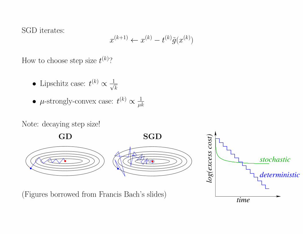
SGD iterates:x(k+1) ← x(k) − t(k)g(x(k))

How to choose step size t(k)?

• Lipschitz case: t(k) ∝ 1√k

• µ-strongly-convex case: t(k) ∝ 1µk

Note: decaying step size!

GD SGD

Stochastic vs. deterministic methods

• Minimizing g(!) =1

n

n!

i=1

fi(!) with fi(!) = ""yi, !

!!(xi)#

+ µ"(!)

• Batch gradient descent: !t = !t"1!#tg#(!t"1) = !t"1!

#t

n

n!

i=1

f #i(!t"1)

• Stochastic gradient descent: !t = !t"1 ! #tf#i(t)(!t"1)

Stochastic vs. deterministic methods

• Minimizing g(!) =1

n

n!

i=1

fi(!) with fi(!) = ""yi, !

!!(xi)#

+ µ"(!)

• Batch gradient descent: !t = !t"1!#tg#(!t"1) = !t"1!

#t

n

n!

i=1

f #i(!t"1)

• Stochastic gradient descent: !t = !t"1 ! #tf#i(t)(!t"1)

Stochastic vs. deterministic methods

• Goal = best of both worlds: linear rate with O(1) iteration cost

timelo

g(ex

cess

cos

t)

stochastic

deterministic

(Figures borrowed from Francis Bach’s slides)

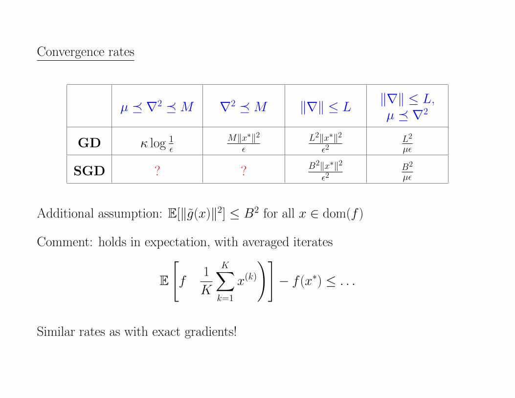
Convergence rates

µ ∇2 M ∇2 M ‖∇‖ ≤ L‖∇‖ ≤ L,µ ∇2

GD κ log 1ε

M‖x∗‖2ε

L2‖x∗‖2ε2

L2

µε

SGD ? ? B2‖x∗‖2ε2

B2

µε

Additional assumption: E[‖g(x)‖2] ≤ B2 for all x ∈ dom(f )

Comment: holds in expectation, with averaged iterates

E

[f

(1

K

K∑

k=1

x(k)

)]− f (x∗) ≤ . . .

Similar rates as with exact gradients!

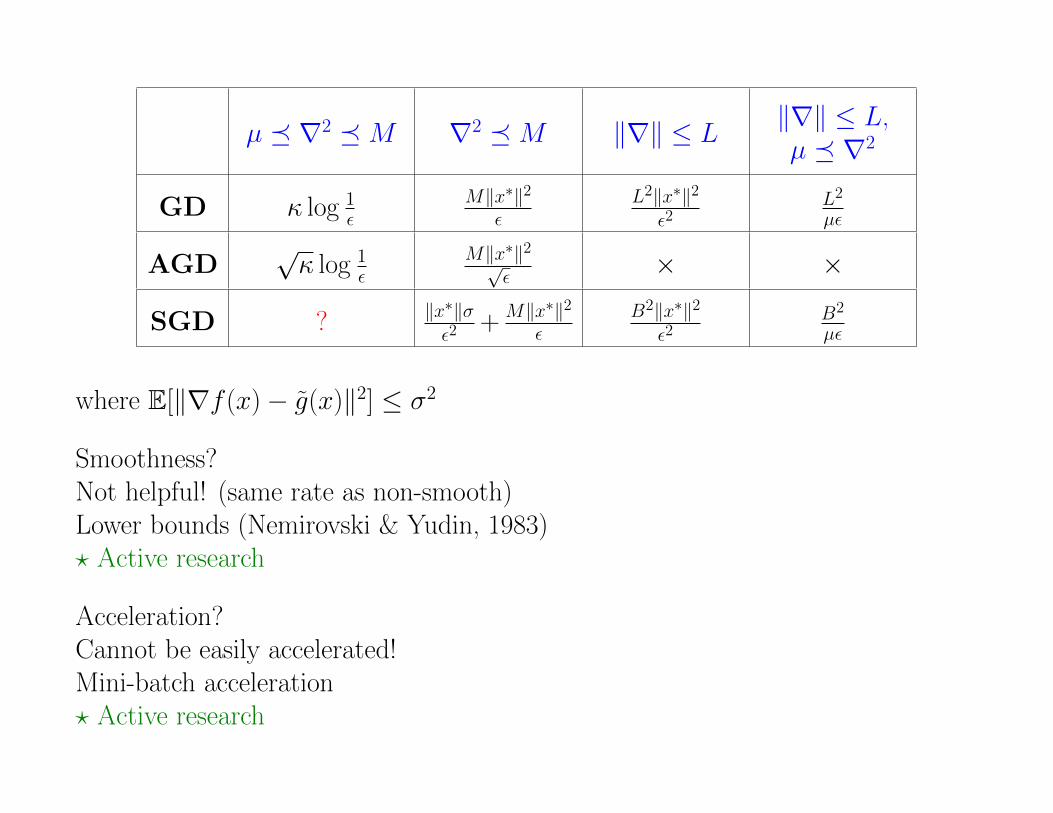
µ ∇2 M ∇2 M ‖∇‖ ≤ L‖∇‖ ≤ L,µ ∇2

GD κ log 1ε

M‖x∗‖2ε

L2‖x∗‖2ε2

L2

µε

AGD√κ log 1

εM‖x∗‖2√

ε× ×

SGD ? ‖x∗‖σε2

+ M‖x∗‖2ε

B2‖x∗‖2ε2

B2

µε

where E[‖∇f (x)− g(x)‖2] ≤ σ2

Smoothness?Not helpful! (same rate as non-smooth)Lower bounds (Nemirovski & Yudin, 1983)? Active research

Acceleration?Cannot be easily accelerated!Mini-batch acceleration? Active research

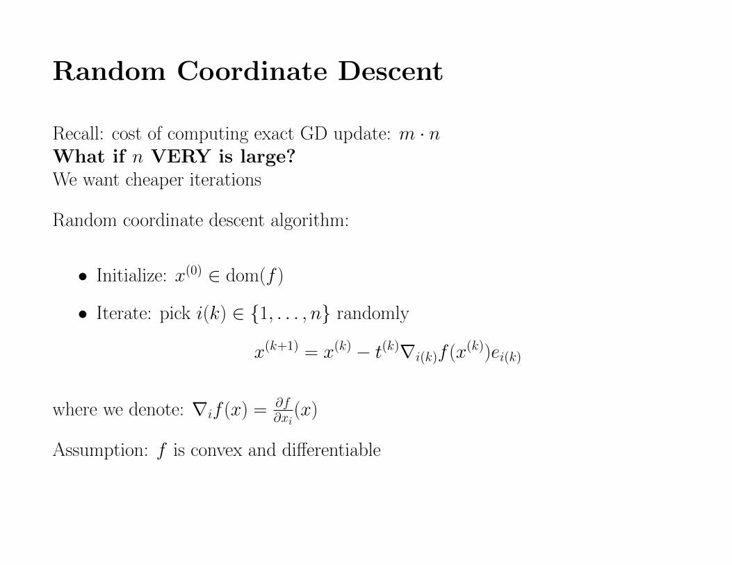
Random Coordinate Descent

Recall: cost of computing exact GD update: m · nWhat if n VERY is large?We want cheaper iterations

Random coordinate descent algorithm:

• Initialize: x(0) ∈ dom(f )

• Iterate: pick i(k) ∈ 1, . . . , n randomly

x(k+1) = x(k) − t(k)∇i(k)f (x(k))ei(k)

where we denote: ∇if (x) = ∂f∂xi

(x)

Assumption: f is convex and differentiable

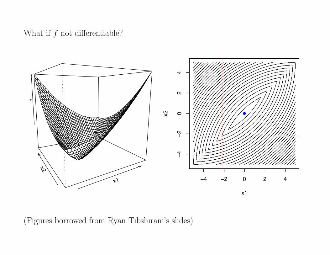
What if f not differentiable?

x1

x2

f

x1

x2

−4 −2 0 2 4−4

−20

24

A: No! Look at the above counterexample

Q: Same question again, but now f (x) = g(x) +Pn

i=1 hi(xi), withg convex, di↵erentiable and each hi convex ... ? (Non-smooth parthere called separable)

5

(Figures borrowed from Ryan Tibshirani’s slides)

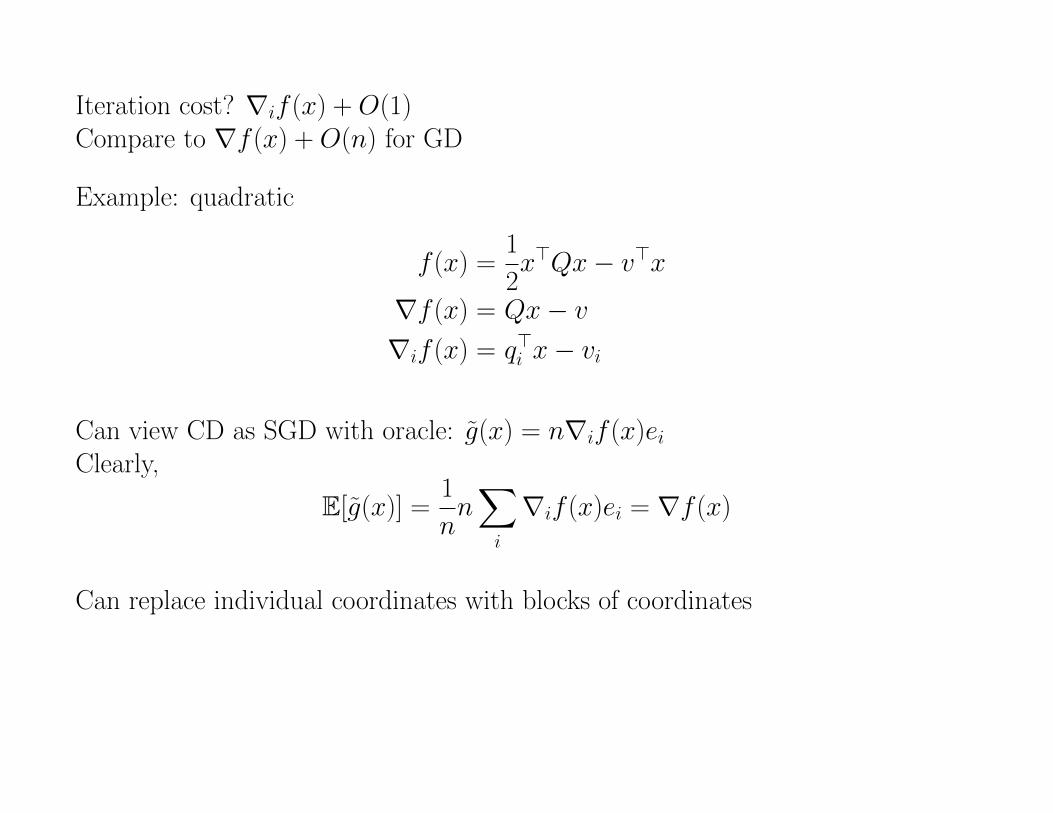
Iteration cost? ∇if (x) + O(1)Compare to ∇f (x) + O(n) for GD

Example: quadratic

f (x) =1

2x>Qx− v>x

∇f (x) = Qx− v∇if (x) = q>i x− vi

Can view CD as SGD with oracle: g(x) = n∇if (x)eiClearly,

E[g(x)] =1

nn∑

i

∇if (x)ei = ∇f (x)

Can replace individual coordinates with blocks of coordinates

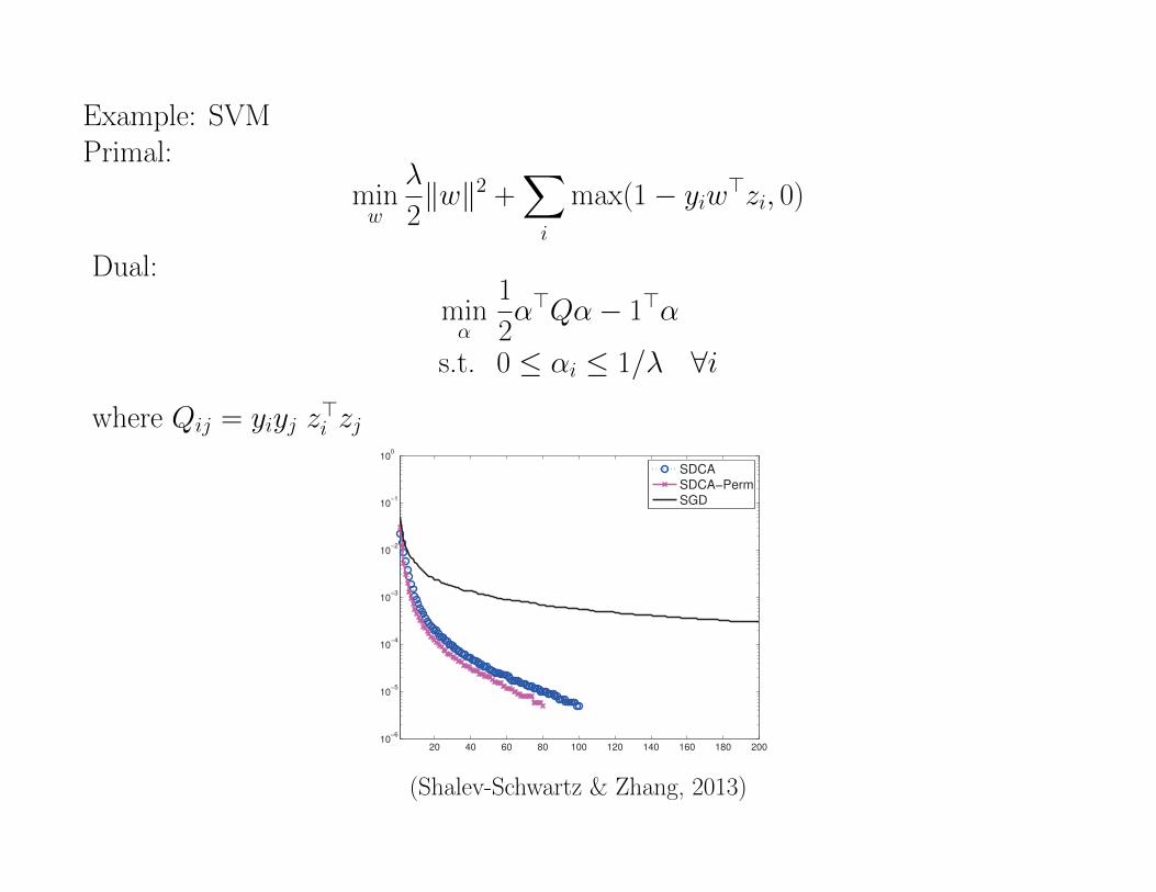
Example: SVMPrimal:

minw

λ

2‖w‖2 +

∑

i

max(1− yiw>zi, 0)

Dual:

minα

1

2α>Qα− 1>α

s.t. 0 ≤ αi ≤ 1/λ ∀iwhere Qij = yiyj z

>i zj

SHALEV-SHWARTZ AND ZHANG

! astro-ph CCAT cov1

10!3

2 4 6 8 10 12 14 16 18 20 2210

!6

10!5

10!4

10!3

10!2

10!1

100

SDCASDCA!PermSGD

2 4 6 8 10 12 14 16 18 20 2210

!6

10!5

10!4

10!3

10!2

10!1

100

SDCASDCA!PermSGD

2 4 6 8 10 12 14 16 18 20 2210

!6

10!5

10!4

10!3

10!2

10!1

100

SDCASDCA!PermSGD

10!4

5 10 15 20 25 30 35 4010

!6

10!5

10!4

10!3

10!2

10!1

100

SDCASDCA!PermSGD

2 4 6 8 10 12 14 16 18 20 2210

!6

10!5

10!4

10!3

10!2

10!1

100

SDCASDCA!PermSGD

2 4 6 8 10 12 14 16 18 20 2210

!6

10!5

10!4

10!3

10!2

10!1

100

SDCASDCA!PermSGD

10!5

10 20 30 40 50 60 70 80 90 100 11010

!6

10!5

10!4

10!3

10!2

10!1

100

SDCASDCA!PermSGD

5 10 15 20 25 30 3510

!6

10!5

10!4

10!3

10!2

10!1

100

SDCASDCA!PermSGD

5 10 15 20 25 3010

!6

10!5

10!4

10!3

10!2

10!1

100

SDCASDCA!PermSGD

10!6

50 100 150 200 250 30010

!6

10!5

10!4

10!3

10!2

10!1

100

SDCASDCA!PermSGD

20 40 60 80 100 120 140 160 180 20010

!6

10!5

10!4

10!3

10!2

10!1

100

SDCASDCA!PermSGD

10 20 30 40 50 60 70 80 90 100 11010

!6

10!5

10!4

10!3

10!2

10!1

100

SDCASDCA!PermSGD

Figure 7: Comparing the primal sub-optimality of SDCA and SGD for the non-smooth hinge-loss(" = 0). In all plots the horizontal axis is the number of iterations divided by training setsize (corresponding to the number of epochs through the data).

596

(Shalev-Schwartz & Zhang, 2013)

Convergence rate

Directional smoothness for f : there exist M1, . . . ,Mn s.t. for any i ∈ 1, . . . , n,x ∈ Rn, and u ∈ R

|∇if (x + uei)−∇if (x)| ≤Mi|u|

Note: implies f is M -smooth with M ≤∑iMi

Consider the update:

x(k+1) = x(k) − 1

Mi(k)∇i(k)f (x(k)) · ei(k)

No need to know Mi’s, can be adjusted dynamically

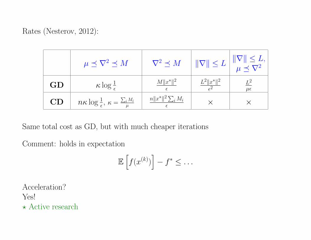
Rates (Nesterov, 2012):

µ ∇2 M ∇2 M ‖∇‖ ≤ L‖∇‖ ≤ L,µ ∇2

GD κ log 1ε

M‖x∗‖2ε

L2‖x∗‖2ε2

L2

µε

CD nκ log 1ε , κ =

∑iMiµ

n‖x∗‖2∑iMiε × ×

Same total cost as GD, but with much cheaper iterations

Comment: holds in expectation

E[f (x(k))

]− f ∗ ≤ . . .

Acceleration?Yes!? Active research