Chapter 1

Overview

Convex OptimizationEuclidean Distance Geometry 2ε

People are so afraid of convex analysis.

−Claude Lemarechal, 2003

In layman’s terms, the mathematical science of Optimization is a study of how to makegood choices when confronted with conflicting requirements and demands. Optimizationis a relatively new wisdom, historically, that can represent balance of real things. Thequalifier convex means: when an optimal solution is found, then it is guaranteed to be abest solution; there is no better choice.

Any convex optimization problem has geometric interpretation. If a given optimizationproblem can be transformed to a convex equivalent, then this interpretive benefit isacquired. That is a powerful attraction: the ability to visualize geometry of anoptimization problem. Conversely, recent advances in geometry and in graph theory holdconvex optimization within their proofs’ core. [433] [337]

This book is about convex optimization, convex geometry (with particular attention todistance geometry), and nonconvex, combinatorial, and geometrical problems that can berelaxed or transformed into convex problems. A virtual flood of new applications followsby epiphany that many problems, presumed nonconvex, can be so transformed: [11] [12][35, §4.3, p.316-322] [61] [97] [162] [165] [294] [316] [324] [380] [381] [430] [433] e.g, sigmadelta analog-to-digital (A/D) audio converter antialiasing (Figure 1).

Euclidean distance geometry is, fundamentally, a determination of point conformation(configuration, relative position or location) by inference from interpoint distanceinformation. By inference we mean: e.g, given only distance information, determinewhether there corresponds a realizable conformation of points; a list of points in somedimension that attains the given interpoint distances. Each point may represent simplylocation or, abstractly, any entity expressible as a vector in finite-dimensional Euclideanspace; e.g, distance geometry of music [114].

Dattorro, Convex Optimization � Euclidean Distance Geometry 2ε, Mεβoo, v2015.07.21. 21

22 CHAPTER 1. OVERVIEW

QΣ

ΣZ-1 -

ternary 1.58bit quantizer

u(t) yi yi

εi

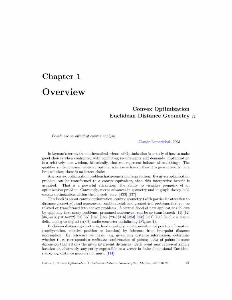
find u

subject to R(y − u) ≤ 131

R(u − y) ≤ 131

Figure 1: Sigma delta quantization is predominant technology [2, p.6] for analog-to-digitalaudio conversion. Input signal u(t) is continuous. Delay z−1 here is analog, perhapsimplemented by sample/hold circuit at MHz rate of yi samples. Observing only y ,samples u can be reconstructed by finding a feasible point in the set of linear inequalitiesrepresenting this coarse quantizer recursion. R is a lower triangular matrix of ones. [104]

b

a = {x |nTj

(

x− s+sj

2

)

= 0}

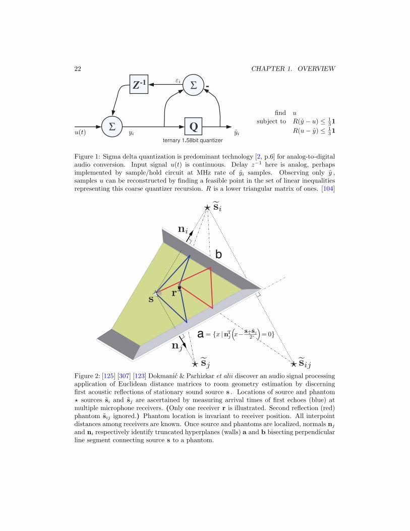
Figure 2: [125] [307] [123] Dokmanic & Parhizkar et alii discover an audio signal processingapplication of Euclidean distance matrices to room geometry estimation by discerningfirst acoustic reflections of stationary sound source s . Locations of source and phantom⋆ sources si and sj are ascertained by measuring arrival times of first echoes (blue) atmultiple microphone receivers. (Only one receiver r is illustrated. Second reflection (red)phantom sij ignored.) Phantom location is invariant to receiver position. All interpointdistances among receivers are known. Once source and phantoms are localized, normals nj

and ni respectively identify truncated hyperplanes (walls) a and b bisecting perpendicularline segment connecting source s to a phantom.

23

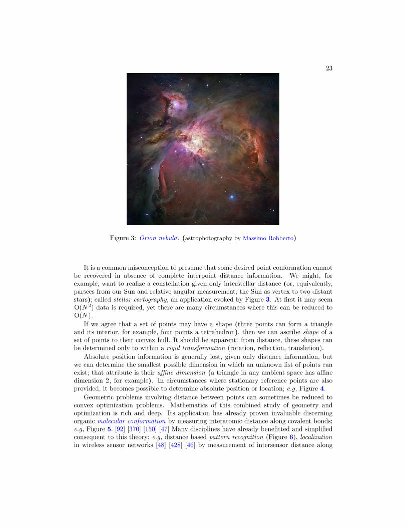
Figure 3: Orion nebula. (astrophotography by Massimo Robberto)

It is a common misconception to presume that some desired point conformation cannotbe recovered in absence of complete interpoint distance information. We might, forexample, want to realize a constellation given only interstellar distance (or, equivalently,parsecs from our Sun and relative angular measurement; the Sun as vertex to two distantstars); called stellar cartography, an application evoked by Figure 3. At first it may seemO(N 2) data is required, yet there are many circumstances where this can be reduced toO(N ).

If we agree that a set of points may have a shape (three points can form a triangleand its interior, for example, four points a tetrahedron), then we can ascribe shape of aset of points to their convex hull. It should be apparent: from distance, these shapes canbe determined only to within a rigid transformation (rotation, reflection, translation).

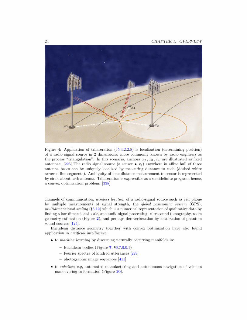
Absolute position information is generally lost, given only distance information, butwe can determine the smallest possible dimension in which an unknown list of points canexist; that attribute is their affine dimension (a triangle in any ambient space has affinedimension 2, for example). In circumstances where stationary reference points are alsoprovided, it becomes possible to determine absolute position or location; e.g, Figure 4.

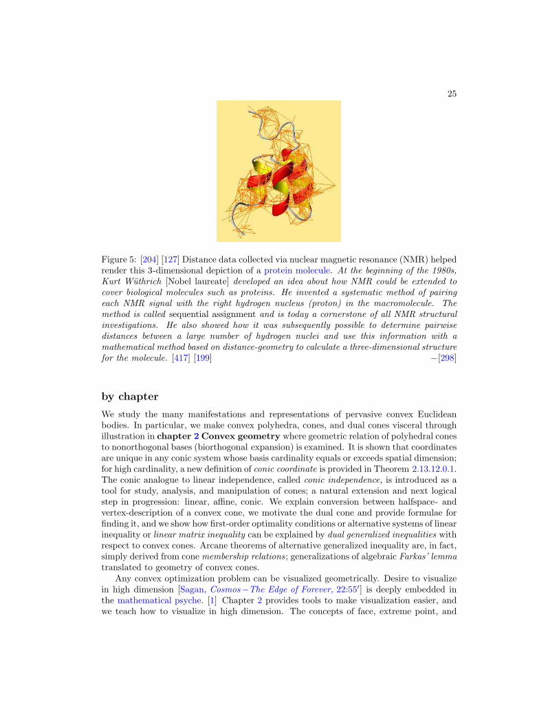
Geometric problems involving distance between points can sometimes be reduced toconvex optimization problems. Mathematics of this combined study of geometry andoptimization is rich and deep. Its application has already proven invaluable discerningorganic molecular conformation by measuring interatomic distance along covalent bonds;e.g, Figure 5. [92] [370] [150] [47] Many disciplines have already benefitted and simplifiedconsequent to this theory; e.g, distance based pattern recognition (Figure 6), localizationin wireless sensor networks [48] [428] [46] by measurement of intersensor distance along

24 CHAPTER 1. OVERVIEW

x2

x4

x3

Figure 4: Application of trilateration (§5.4.2.2.8) is localization (determining position)of a radio signal source in 2 dimensions; more commonly known by radio engineers asthe process “triangulation”. In this scenario, anchors x2 , x3 , x4 are illustrated as fixedantennae. [225] The radio signal source (a sensor • x1) anywhere in affine hull of threeantenna bases can be uniquely localized by measuring distance to each (dashed whitearrowed line segments). Ambiguity of lone distance measurement to sensor is representedby circle about each antenna. Trilateration is expressible as a semidefinite program; hence,a convex optimization problem. [338]

channels of communication, wireless location of a radio-signal source such as cell phoneby multiple measurements of signal strength, the global positioning system (GPS),multidimensional scaling (§5.12) which is a numerical representation of qualitative data byfinding a low-dimensional scale, and audio signal processing: ultrasound tomography, roomgeometry estimation (Figure 2), and perhaps dereverberation by localization of phantomsound sources [124].

Euclidean distance geometry together with convex optimization have also foundapplication in artificial intelligence:

� to machine learning by discerning naturally occurring manifolds in:

– Euclidean bodies (Figure 7, §6.7.0.0.1)

– Fourier spectra of kindred utterances [228]

– photographic image sequences [411]

� to robotics; e.g, automated manufacturing and autonomous navigation of vehiclesmaneuvering in formation (Figure 10).

25

Figure 5: [204] [127] Distance data collected via nuclear magnetic resonance (NMR) helpedrender this 3-dimensional depiction of a protein molecule. At the beginning of the 1980s,Kurt Wuthrich [Nobel laureate] developed an idea about how NMR could be extended tocover biological molecules such as proteins. He invented a systematic method of pairingeach NMR signal with the right hydrogen nucleus (proton) in the macromolecule. Themethod is called sequential assignment and is today a cornerstone of all NMR structuralinvestigations. He also showed how it was subsequently possible to determine pairwisedistances between a large number of hydrogen nuclei and use this information with amathematical method based on distance-geometry to calculate a three-dimensional structurefor the molecule. [417] [199] −[298]

by chapter

We study the many manifestations and representations of pervasive convex Euclideanbodies. In particular, we make convex polyhedra, cones, and dual cones visceral throughillustration in chapter 2 Convex geometry where geometric relation of polyhedral conesto nonorthogonal bases (biorthogonal expansion) is examined. It is shown that coordinatesare unique in any conic system whose basis cardinality equals or exceeds spatial dimension;for high cardinality, a new definition of conic coordinate is provided in Theorem 2.13.12.0.1.The conic analogue to linear independence, called conic independence, is introduced as atool for study, analysis, and manipulation of cones; a natural extension and next logicalstep in progression: linear, affine, conic. We explain conversion between halfspace- andvertex-description of a convex cone, we motivate the dual cone and provide formulae forfinding it, and we show how first-order optimality conditions or alternative systems of linearinequality or linear matrix inequality can be explained by dual generalized inequalities withrespect to convex cones. Arcane theorems of alternative generalized inequality are, in fact,simply derived from cone membership relations; generalizations of algebraic Farkas’ lemmatranslated to geometry of convex cones.

Any convex optimization problem can be visualized geometrically. Desire to visualizein high dimension [Sagan, Cosmos−The Edge of Forever, 22:55′] is deeply embedded inthe mathematical psyche. [1] Chapter 2 provides tools to make visualization easier, andwe teach how to visualize in high dimension. The concepts of face, extreme point, and

26 CHAPTER 1. OVERVIEW

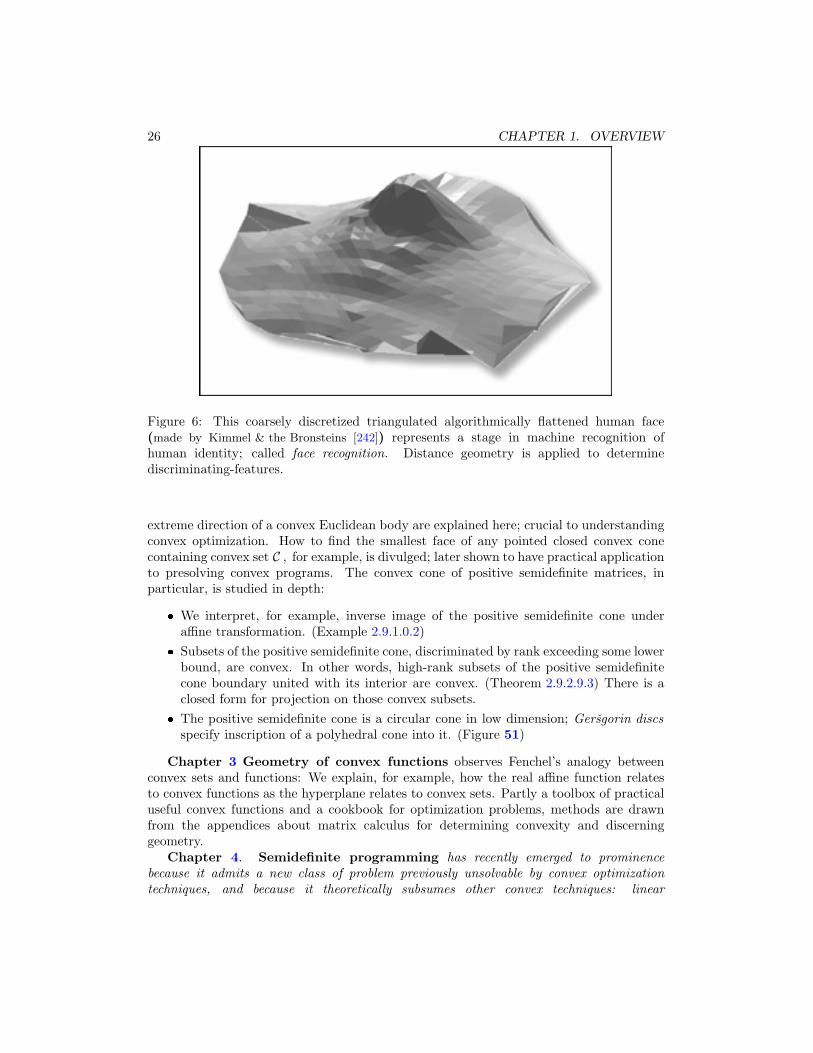
Figure 6: This coarsely discretized triangulated algorithmically flattened human face(made by Kimmel & the Bronsteins [242]) represents a stage in machine recognition ofhuman identity; called face recognition. Distance geometry is applied to determinediscriminating-features.

extreme direction of a convex Euclidean body are explained here; crucial to understandingconvex optimization. How to find the smallest face of any pointed closed convex conecontaining convex set C , for example, is divulged; later shown to have practical applicationto presolving convex programs. The convex cone of positive semidefinite matrices, inparticular, is studied in depth:

� We interpret, for example, inverse image of the positive semidefinite cone underaffine transformation. (Example 2.9.1.0.2)

� Subsets of the positive semidefinite cone, discriminated by rank exceeding some lowerbound, are convex. In other words, high-rank subsets of the positive semidefinitecone boundary united with its interior are convex. (Theorem 2.9.2.9.3) There is aclosed form for projection on those convex subsets.

� The positive semidefinite cone is a circular cone in low dimension; Gersgorin discsspecify inscription of a polyhedral cone into it. (Figure 51)

Chapter 3 Geometry of convex functions observes Fenchel’s analogy betweenconvex sets and functions: We explain, for example, how the real affine function relatesto convex functions as the hyperplane relates to convex sets. Partly a toolbox of practicaluseful convex functions and a cookbook for optimization problems, methods are drawnfrom the appendices about matrix calculus for determining convexity and discerninggeometry.

Chapter 4. Semidefinite programming has recently emerged to prominencebecause it admits a new class of problem previously unsolvable by convex optimizationtechniques, and because it theoretically subsumes other convex techniques: linear

27

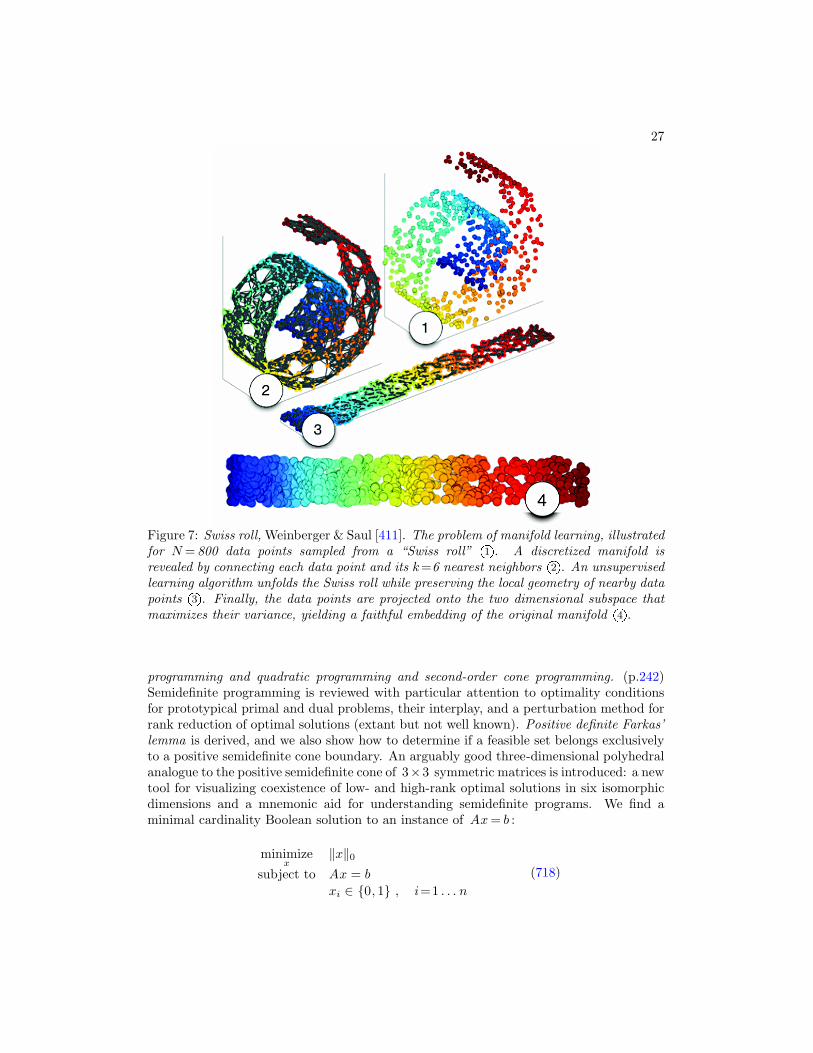
Figure 7: Swiss roll, Weinberger & Saul [411]. The problem of manifold learning, illustratedfor N = 800 data points sampled from a “Swiss roll” 1

O. A discretized manifold isrevealed by connecting each data point and its k=6 nearest neighbors 2

O. An unsupervisedlearning algorithm unfolds the Swiss roll while preserving the local geometry of nearby datapoints 3

O. Finally, the data points are projected onto the two dimensional subspace thatmaximizes their variance, yielding a faithful embedding of the original manifold 4

O.

programming and quadratic programming and second-order cone programming. (p.242)Semidefinite programming is reviewed with particular attention to optimality conditionsfor prototypical primal and dual problems, their interplay, and a perturbation method forrank reduction of optimal solutions (extant but not well known). Positive definite Farkas’lemma is derived, and we also show how to determine if a feasible set belongs exclusivelyto a positive semidefinite cone boundary. An arguably good three-dimensional polyhedralanalogue to the positive semidefinite cone of 3×3 symmetric matrices is introduced: a newtool for visualizing coexistence of low- and high-rank optimal solutions in six isomorphicdimensions and a mnemonic aid for understanding semidefinite programs. We find aminimal cardinality Boolean solution to an instance of Ax = b :

minimizex

‖x‖0

subject to Ax = b

xi ∈ {0, 1} , i=1 . . . n

(718)

28 CHAPTER 1. OVERVIEW

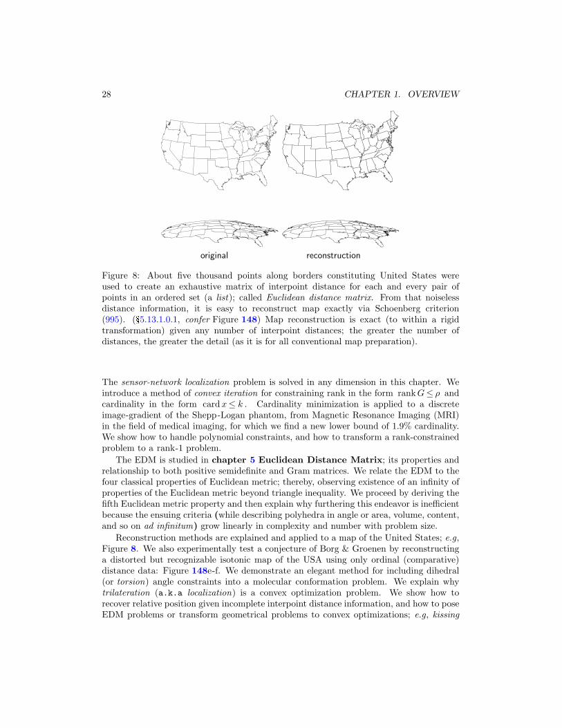
original reconstruction

Figure 8: About five thousand points along borders constituting United States wereused to create an exhaustive matrix of interpoint distance for each and every pair ofpoints in an ordered set (a list); called Euclidean distance matrix. From that noiselessdistance information, it is easy to reconstruct map exactly via Schoenberg criterion(995). (§5.13.1.0.1, confer Figure 148) Map reconstruction is exact (to within a rigidtransformation) given any number of interpoint distances; the greater the number ofdistances, the greater the detail (as it is for all conventional map preparation).

The sensor-network localization problem is solved in any dimension in this chapter. Weintroduce a method of convex iteration for constraining rank in the form rankG≤ ρ andcardinality in the form cardx≤ k . Cardinality minimization is applied to a discreteimage-gradient of the Shepp-Logan phantom, from Magnetic Resonance Imaging (MRI)in the field of medical imaging, for which we find a new lower bound of 1.9% cardinality.We show how to handle polynomial constraints, and how to transform a rank-constrainedproblem to a rank-1 problem.

The EDM is studied in chapter 5 Euclidean Distance Matrix; its properties andrelationship to both positive semidefinite and Gram matrices. We relate the EDM to thefour classical properties of Euclidean metric; thereby, observing existence of an infinity ofproperties of the Euclidean metric beyond triangle inequality. We proceed by deriving thefifth Euclidean metric property and then explain why furthering this endeavor is inefficientbecause the ensuing criteria (while describing polyhedra in angle or area, volume, content,and so on ad infinitum) grow linearly in complexity and number with problem size.

Reconstruction methods are explained and applied to a map of the United States; e.g,Figure 8. We also experimentally test a conjecture of Borg & Groenen by reconstructinga distorted but recognizable isotonic map of the USA using only ordinal (comparative)distance data: Figure 148e-f. We demonstrate an elegant method for including dihedral(or torsion) angle constraints into a molecular conformation problem. We explain whytrilateration (a.k.a localization) is a convex optimization problem. We show how torecover relative position given incomplete interpoint distance information, and how to poseEDM problems or transform geometrical problems to convex optimizations; e.g, kissing

29

(a) (b)

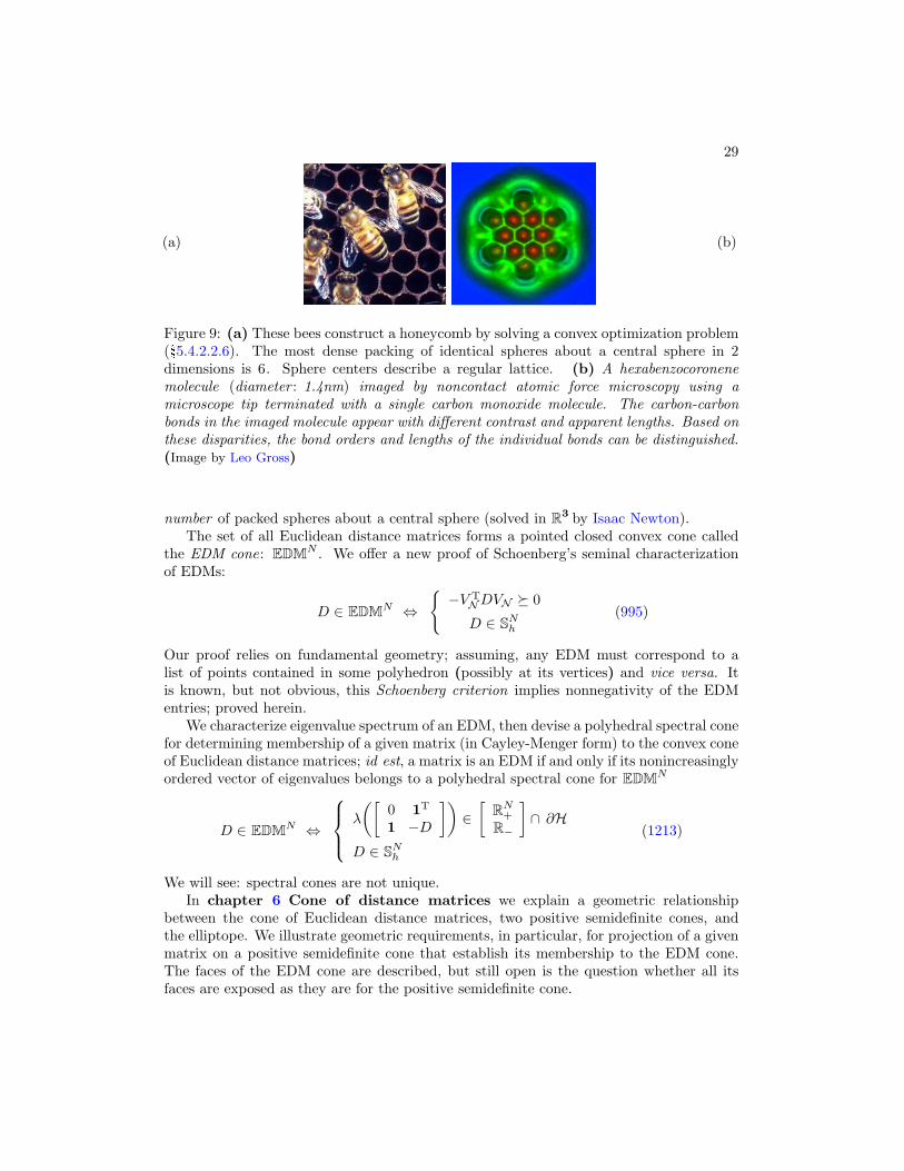
Figure 9: (a) These bees construct a honeycomb by solving a convex optimization problem(§5.4.2.2.6). The most dense packing of identical spheres about a central sphere in 2dimensions is 6. Sphere centers describe a regular lattice. (b) A hexabenzocoronenemolecule (diameter : 1.4nm) imaged by noncontact atomic force microscopy using amicroscope tip terminated with a single carbon monoxide molecule. The carbon-carbonbonds in the imaged molecule appear with different contrast and apparent lengths. Based onthese disparities, the bond orders and lengths of the individual bonds can be distinguished.(Image by Leo Gross)

number of packed spheres about a central sphere (solved in R3 by Isaac Newton).The set of all Euclidean distance matrices forms a pointed closed convex cone called

the EDM cone: EDMN . We offer a new proof of Schoenberg’s seminal characterizationof EDMs:

D ∈ EDMN ⇔{

−V TNDVN º 0

D ∈ SNh

(995)

Our proof relies on fundamental geometry; assuming, any EDM must correspond to alist of points contained in some polyhedron (possibly at its vertices) and vice versa. Itis known, but not obvious, this Schoenberg criterion implies nonnegativity of the EDMentries; proved herein.

We characterize eigenvalue spectrum of an EDM, then devise a polyhedral spectral conefor determining membership of a given matrix (in Cayley-Menger form) to the convex coneof Euclidean distance matrices; id est, a matrix is an EDM if and only if its nonincreasinglyordered vector of eigenvalues belongs to a polyhedral spectral cone for EDMN

D ∈ EDMN ⇔

λ

([

0 1T

1 −D

])

∈[

RN+

R−

]

∩ ∂H

D ∈ SNh

(1213)

We will see: spectral cones are not unique.In chapter 6 Cone of distance matrices we explain a geometric relationship

between the cone of Euclidean distance matrices, two positive semidefinite cones, andthe elliptope. We illustrate geometric requirements, in particular, for projection of a givenmatrix on a positive semidefinite cone that establish its membership to the EDM cone.The faces of the EDM cone are described, but still open is the question whether all itsfaces are exposed as they are for the positive semidefinite cone.

30 CHAPTER 1. OVERVIEW

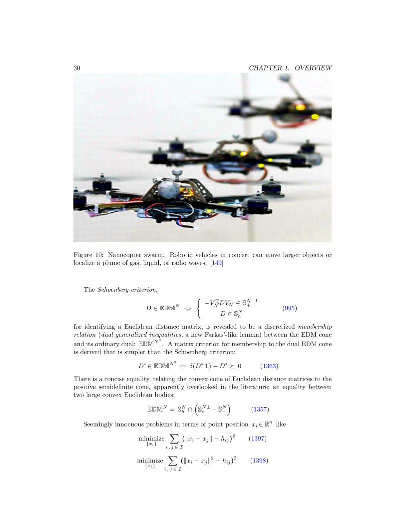
Figure 10: Nanocopter swarm. Robotic vehicles in concert can move larger objects orlocalize a plume of gas, liquid, or radio waves. [149]

The Schoenberg criterion,

D ∈ EDMN ⇔{

−V TNDVN ∈ SN−1

+

D ∈ SNh

(995)

for identifying a Euclidean distance matrix, is revealed to be a discretized membershiprelation (dual generalized inequalities, a new Farkas’-like lemma) between the EDM cone

and its ordinary dual: EDMN∗. A matrix criterion for membership to the dual EDM cone

is derived that is simpler than the Schoenberg criterion:

D∗∈ EDMN∗ ⇔ δ(D∗ 1) − D∗ º 0 (1363)

There is a concise equality, relating the convex cone of Euclidean distance matrices to thepositive semidefinite cone, apparently overlooked in the literature; an equality betweentwo large convex Euclidean bodies:

EDMN = SNh ∩

(

SN⊥c − SN

+

)

(1357)

Seemingly innocuous problems in terms of point position xi∈ Rn like

minimize{xi}

∑

i , j ∈ I(‖xi − xj‖ − hij)

2(1397)

minimize{xi}

∑

i , j ∈ I(‖xi − xj‖2 − hij)

2(1398)

31

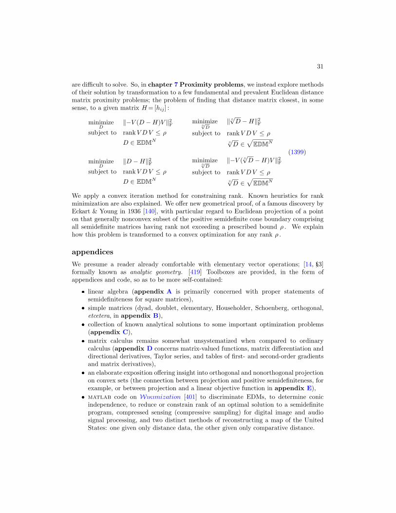
are difficult to solve. So, in chapter 7 Proximity problems, we instead explore methodsof their solution by transformation to a few fundamental and prevalent Euclidean distancematrix proximity problems; the problem of finding that distance matrix closest, in somesense, to a given matrix H = [hij ] :

minimizeD

‖−V (D − H)V ‖2F

subject to rankV D V ≤ ρ

D ∈ EDMN

minimize◦√

D‖ ◦√

D − H‖2F

subject to rankV D V ≤ ρ◦√

D ∈√

EDMN

minimizeD

‖D − H‖2F

subject to rankV D V ≤ ρ

D ∈ EDMN

minimize◦√

D‖−V ( ◦

√D − H)V ‖2

F

subject to rankV D V ≤ ρ◦√

D ∈√

EDMN

(1399)

We apply a convex iteration method for constraining rank. Known heuristics for rankminimization are also explained. We offer new geometrical proof, of a famous discovery byEckart & Young in 1936 [140], with particular regard to Euclidean projection of a pointon that generally nonconvex subset of the positive semidefinite cone boundary comprisingall semidefinite matrices having rank not exceeding a prescribed bound ρ . We explainhow this problem is transformed to a convex optimization for any rank ρ .

appendices

We presume a reader already comfortable with elementary vector operations; [14, §3]formally known as analytic geometry. [419] Toolboxes are provided, in the form ofappendices and code, so as to be more self-contained:

� linear algebra (appendix A is primarily concerned with proper statements ofsemidefiniteness for square matrices),

� simple matrices (dyad, doublet, elementary, Householder, Schoenberg, orthogonal,etcetera, in appendix B),

� collection of known analytical solutions to some important optimization problems(appendix C),

� matrix calculus remains somewhat unsystematized when compared to ordinarycalculus (appendix D concerns matrix-valued functions, matrix differentiation anddirectional derivatives, Taylor series, and tables of first- and second-order gradientsand matrix derivatives),

� an elaborate exposition offering insight into orthogonal and nonorthogonal projectionon convex sets (the connection between projection and positive semidefiniteness, forexample, or between projection and a linear objective function in appendix E),

� matlab code on Wıκımization [401] to discriminate EDMs, to determine conicindependence, to reduce or constrain rank of an optimal solution to a semidefiniteprogram, compressed sensing (compressive sampling) for digital image and audiosignal processing, and two distinct methods of reconstructing a map of the UnitedStates: one given only distance data, the other given only comparative distance.

32 CHAPTER 1. OVERVIEW

Figure 11: Three-dimensional reconstruction of David from distance data.

Figure 12: Digital Michelangelo Project , Stanford University. Measuring distance to Davidby laser rangefinder. Spatial resolution is 0.29mm.