ULTRAMETRIC SUBSETS WITH LARGE HAUSDORFF DIMENSION

MANOR MENDEL AND ASSAF NAOR

Abstract. It is shown that for every ε ∈ (0, 1), every compact metric space (X, d) has acompact subset S ⊆ X that embeds into an ultrametric space with distortion O(1/ε), and

dimH(S) > (1− ε) dimH(X),

where dimH(·) denotes Hausdorff dimension. The above O(1/ε) distortion estimate is shownto be sharp via a construction based on sequences of expander graphs.

Contents

1. Introduction 21.1. An overview of the proof of Theorem 1.5 41.2. The low distortion regime 51.3. Further applications 61.3.1. Urbanski’s problem 61.3.2. Talagrand’s majorizing measures theorem 72. Reduction to finite metric spaces 83. Combinatorial trees and fragmentation maps 114. From fragmentation maps to covering theorems 135. Asymptotically optimal fragmentation maps: proof of Lemma 4.3 156. An intermediate fragmentation map: proof of Lemma 5.5 227. The initial fragmentation map: proof of Lemma 6.2 258. An iterated Holder argument for trees: proof of Lemma 6.5 279. Proof of Theorem 5.3 3310. Impossibility results 3510.1. Trees of metric spaces 3510.2. Expander fractals 3910.3. G (n, 1/2) fractals 39References 40

2010 Mathematics Subject Classification. 30L05,46B85,37F35.Key words and phrases. Bi-Lipschitz embeddings, Hausdorff dimension, ultrametrics, Dvoretzky’s

theorem.M. M. was partially supported by ISF grants 221/07 and 93/11, BSF grants 2006009 and 2010021, and

a gift from Cisco Research Center. A. N. was partially supported by NSF grant CCF-0832795, BSF grants2006009 and 2010021, and the Packard Foundation. Part of this work was completed when M. M. wasvisiting Microsoft Research and University of Washington, and A. N. was visiting the Discrete Analysisprogram at the Isaac Newton Institute for Mathematical Sciences and the Quantitative Geometry programat the Mathematical Sciences Research Institute.

1

1. Introduction

Given D > 1, a metric space (X, dX) is said to embed with distortion D into a metricspace (Y, dY ) if there exists f : X → Y and λ > 0 such that for all x, y ∈ X we have

λdX(x, y) 6 dY (f(x), f(y)) 6 DλdX(x, y). (1)

Note that when Y is a Banach space the scaling factor λ can be dropped in the definition (1).Answering positively a conjecture of Grothendieck [15], Dvoretzky proved [13] that for

every k ∈ N and D > 1 there exists n = n(k,D) ∈ N such that every n-dimensional normedspace has a k-dimensional linear subspace that embeds into Hilbert space with distortion D;see [28, 27, 32] for the best known bounds on n(k,D).

Bourgain, Figiel and Milman [9] studied the following problem as a natural nonlinearvariant of Dvoretzky’s theorem: given n ∈ N and D > 1, what is the largest m ∈ N suchthat any finite metric space (X, d) of cardinality n has a subset S ⊆ X with |S| > msuch that the metric space (S, d) embeds with distortion D into Hilbert space? Denote thisvalue of m by R(n,D). Bourgain-Figiel-Milman proved [9] that for all D > 1 there existsc(D) ∈ (0,∞) such that R(n,D) > c(D) log n, and that R(n, 1.023) = O(log n). Followingseveral investigations [18, 8, 3] that were motivated by algorithmic applications, a morecomplete description of the Bourgain-Figiel-Milman phenomenon was obtained in [5].

Theorem 1.1 ([5]). For D ∈ (1,∞) there exist c(D), c′(D) ∈ (0,∞) and δ(D), δ′(D) ∈ (0, 1)such that for every n ∈ N,

• if D ∈ (1, 2) then c(D) log n 6 R(n,D) 6 c′(D) log n,• if D ∈ (2,∞) then n1−δ(D) 6 R(n,D) 6 n1−δ′(D).

Highlighting the case of large D, which is most relevant for applications, we have thefollowing theorem.

Theorem 1.2 ([5, 25, 30]). For every ε ∈ (0, 1) and n ∈ N, any n-point metric space (X, d)has a subset S ⊆ X with |S| > n1−ε that embeds into an ultrametric space with distortion2e/ε. On the other hand, there exists a universal constant c > 0 with the following property.For every n ∈ N there is an n-point metric space Xn such that for every ε ∈ (0, 1) all subsetsY ⊆ X with |Y | > n1−ε incur distortion at least c/ε in any embedding into Hilbert space.

Recall that a metric space (U, ρ) is called an ultrametric space if for every x, y, z ∈ U wehave ρ(x, y) 6 max {ρ(x, z), ρ(z, y)}. Any separable ultrametric space admits an isometricembedding into Hilbert space [39]. Hence the subset S from Theorem 1.2 also embeds withthe stated distortion into Hilbert space, and therefore Theorem 1.2 fits into the Bourgain-Figiel-Milman framework. Note, however, that the stronger statement that S embeds intoan ultrametric space is needed for the applications in [5, 25], and that the matching lowerbound in Theorem 1.2 is for the weaker requirement of embeddability into Hilbert space.Thus, a byproduct of Theorem 1.2 is the assertion that, in general, the best way (up toconstant factors) to find a large approximately Euclidean subset is to actually find a subsetsatisfying the more stringent requirement of being almost ultrametric. The existence ofthe metric spaces {Xn}∞n=1 from Theorem 1.2 was established in [5]. The estimate 2e/ε onthe ultrametric distortion of the subset S from Theorem 1.2 is due to [30], improving by aconstant factor over the bound from [25], which itself improves (in an asymptotically optimalway) on the distortion bound of O (ε−1 log(2/ε)) from [5].

2

In what follows, dimH(X) denotes the Hausdorff dimension of a metric space X. Inspiredby the above theorems, Terence Tao proposed (unpublished, 2006) another natural variantof the nonlinear Dvoretzky problem: one can keep the statement of Dvoretzky’s theoremunchanged in the context of general metric spaces, while interpreting the notion of dimensionin the appropriate category. Thus one arrives at the following question.

Question 1.3 (The nonlinear Dvoretzky problem for Hausdorff dimension). Given α > 0and D > 1, what is the supremum over those β > 0 with the following property. Everycompact metric space X with dimH(X) > α has a subset S ⊆ X with dimH(S) > β thatembeds into Hilbert space with distortion D?

The restriction of Question 1.3 to compact metric spaces is not severe. For example, ifX is complete and separable then one can first pass to a compact subset of X with thesame Hausdorff dimension, and even the completeness of X can be replaced by weakerassumptions; see [11, 16]. We will not address this issue here and restrict our discussion tocompact metric spaces, where the crucial subtleties of the problem are already present.

Our purpose here is to provide answers to Question 1.3 in various distortion regimes, themain result being the following theorem.

Theorem 1.4. There exists a universal constant C ∈ (0,∞) such that for every ε ∈ (0, 1)and α ∈ (0,∞), every compact metric space X with dimH(X) > α has a closed subset S ⊆ Xwith dimH(S) > (1− ε)α that embeds with distortion C/ε into an ultrametric space. In thereverse direction, there is a universal constant c > 0 such that for every α > 0 there exists acompact metric space Xα with dimH(Xα) = α such that if S ⊆ X satisfies dimH(S) > (1−ε)αthen S incurs distortion at least c/ε in any embedding into Hilbert space.

The construction of the spaces Xα from Theorem 1.4 builds on the examples of [5], whichare based on expander graphs. The limiting spaces Xα obtained this way can therefore becalled “expander fractals”; their construction is discussed in Section 10.

Our main new contribution leading to Theorem 1.4 is the following structural result forgeneral metric measure spaces. In what follows, by a metric measure space (X, d, µ) we meana compact metric space (X, d), equipped with a Borel measure µ such that µ(X) <∞. Forr > 0 and x ∈ X, the corresponding closed ball is denoted B(x, r) = {y ∈ X : d(x, y) 6 r}.

Theorem 1.5. For every ε ∈ (0, 1) there exists cε ∈ (0,∞) with the following property.Every metric measure space (X, d, µ) has a closed subset S ⊆ X such that (S, d) embeds intoan ultrametric space with distortion 9/ε, and for every {xi}i∈I ⊆ X and {ri}i∈I ⊆ [0,∞)such that the balls {B(xi, ri)}i∈I cover S, i.e.,⋃

i∈I

B(xi, ri) ⊇ S, (2)

we have ∑i∈I

µ(B(xi, cεri))1−ε > µ(X)1−ε. (3)

Theorem 1.5 contains Theorem 1.2 as a simple special case. Indeed, consider the casewhen X is finite, say |X| = n, the measure µ is the counting measure, i.e., µ(A) = |A|for all A ⊆ X, and all the radii {ri}i∈I vanish. In this case B(xi, ri) = B(xi, cεri) = {xi},and therefore the covering condition (2) implies that {xi}i∈I ⊇ S. Inequality (3) therefore

3

implies that |S| > n1−ε, which is the (asymptotically sharp) conclusion of Theorem 1.2, upto a constant multiplicative factor in the distortion.

Theorem 1.5 also implies Theorem 1.4. To see this assume that (X, d) is a compactmetric space and dimH(X) > α. The Frostman lemma (see [16] and [24, Ch. 8]) impliesthat there exists a constant K ∈ (0,∞) and a Borel measure µ such that µ(X) > 0 andµ(B(x, r)) 6 Krα for all r > 0 and x ∈ X. An application of Theorem 1.5 to the metricmeasure space (X, d, µ) yields a closed subset S ⊆ X that embeds into an ultrametric spacewith distortion O(1/ε) and satisfies the covering condition (3). Thus, all the covers of S byballs {B(xi, ri)}i∈I satisfy

µ(X)1−ε 6∑i∈I

µ(B(xi, cεri))1−ε 6

∑i∈I

(Kcαε rαi )1−ε .

Hence, ∑i∈I

r(1−ε)αi >

µ(X)1−ε

K1−εc(1−ε)αε

.

This means that the (1− ε)α-Hausdorff content1 of S satisfies

H(1−ε)α∞ (S) >

µ(X)1−ε

K1−εc(1−ε)αε

> 0,

and therefore dimH(S) = inf{β > 0 : Hβ

∞(S) = 0}> (1− ε)α, as asserted in Theorem 1.4.

To summarize the above discussion, the general structural result for metric measure spacesthat is contained in Theorem 1.5 implies the sharp Bourgain-Figiel-Milman style nonlinearDvoretzky theorem when applied to trivial covers of S by singletons. The nonlinear Dvoret-zky problem for Hausdorff dimension is more subtle since one has to argue about all possiblecovers of S, and this is achieved by applying Theorem 1.5 to the metric measure space in-duced by a Frostman measure. In both of these applications the value of the constant cε inTheorem 1.5 is irrelevant, but we anticipate that it will play a role in future applications ofTheorem 1.5. Our argument yields the bound cε = eO(1/ε2), but we have no reason to believethat this dependence on ε is optimal. We therefore pose the following natural problem.

Question 1.6. What is the asymptotic behavior as ε → 0 of the best possible constant cεin Theorem 1.5?

1.1. An overview of the proof of Theorem 1.5. Theorem 1.1 was proved in [5] via adeterministic iterative construction of a sufficiently large almost ultrametric subset S of agiven finite metric space (X, d). In contrast, Theorem 1.2 was proved in [25] via a significantlyshorter probabilistic argument. It is shown in [25] how to specify a distribution (dependingon the geometry of X) over random subsets S ⊆ X that embed into an ultrametric space withsmall distortion, yet their expected cardinality is large. The lower bound on the expectedcardinality of S is obtained via a lower bound on the probability Pr [x ∈ S] for each x ∈ X.Such a probabilistic estimate seems to be quite special, and we do not see how to argueprobabilistically about all possible covers of a random subset S, as required in Theorem 1.5.In other words, a reason why Question 1.3 is more subtle than the Bourgain-Figiel-Milmanproblem is that ensuring that S is large is in essence a local requirement, while ensuring that

1Recall that for β > 0 the β-Hausdorff content of a metric space (Z, d) is defined to be the infimum of∑j∈J r

βj over all possible covers of Z by balls {B(zj , rj)}j∈J ; see [24].

4

S is high-dimensional is a global requirement: once S has been determined one has to argueabout all possible covers of S rather than estimating Pr [x ∈ S] for each x ∈ X separately.

For the above reason our proof of Theorem 1.5 is a deterministic construction which uses insome of its steps adaptations of the methods of [5], in addition to a variety of new ingredientsthat are needed in order to handle a covering condition such as (3). Actually, in order toobtain the sharp O(1/ε) distortion bound of Theorem 1.5 we also use results of [25, 30] (seeTheorem 9.1 below), so in fact Theorem 1.5 is based on a combination of deterministic andprobabilistic methods, the deterministic steps being the most substantial new contribution.

The proof of Theorem 1.5 starts with a reduction of the problem to the case of finite metricspaces; see Section 2. Once this is achieved, the argument is a mixture of combinatorial,analytic and geometric arguments, the key objects of interest being fragmentation maps.These are maps that are defined on rooted combinatorial trees and assign to each vertex ofthe tree a subset of the metric space (X, d) in a way that respects the tree structure, i.e.,the set corresponding to an offspring of a vertex is a subset of the set corresponding to thevertex itself, and vertices lying on distinct root-leaf paths are assigned to disjoint subsets ofX. We also require that leaves are mapped to singletons.

Each fragmentation map corresponds to a subset of X (the images of the leaves), and ourgoal is to produce a fragmentation map that corresponds to a subset of X which satisfies theconclusion of Theorem 1.5. To this end, we initiate the iteration via a bottom-up constructionof a special fragmentation map; see Section 7. We then proceed to iteratively “prune” (or“sparsify”) this initial tree so as to produce a smaller tree whose leaves satisfy the conclusionof Theorem 1.5. At each step we argue that there must exist sufficiently many good pruninglocations so that by a pigeonhole argument we can make the successive pruning locationsalign appropriately; see Section 8.

At this point, the subset corresponding to fragmentation map that we constructed issufficient to prove Theorem 1.5 with a weaker bound of eO(1/ε2) on its ultrametric distortion;see Remark 5.6. To get the optimal distortion we add another pruning step guided by aweighted version (proved in Section 9) of the nonlinear Dvoretzky theorem for finite metricspaces. The mechanism of this second type of pruning is described in Section 5.

It is impossible to describe the exact details of the above steps without introducing asignificant amount of notation and terminology, and specifying rather complicated inductivehypotheses. We therefore refer to the relevant sections for a detailed description. To helpmotivate the lengthy arguments, in the body of this paper we present the proof in a top-downfashion which is opposite to the order in which it was described above.

1.2. The low distortion regime. We have thus far focused on Question 1.3 in the case ofhigh distortion embeddings into ultrametric spaces. There is also a Hausdorff dimensionalvariant of the phase transition at distortion 2 that was described in Theorem 1.1.

Theorem 1.7 (Distortion 2 + δ). There exists a universal constant c ∈ (0,∞) such thatfor every δ ∈ (0, 1/2), any compact metric space (X, d) of finite Hausdorff dimension has aclosed subset S ⊆ X that embeds with distortion 2 + δ in an ultrametric space, and

dimH(S) >cδ

log(1/δ)dimH(X). (4)

For distortion strictly less than 2 the following theorem shows that there is no nonlinearDvoretzky phenomenon in terms of Hausdorff dimension.

5

Theorem 1.8. For every α ∈ (0,∞) there exists a compact metric space (X, d) of Hausdorffdimension α, such that if S ⊆ X embeds into Hilbert space with distortion strictly smallerthan 2 then dimH(S) = 0.

It was recently observed in [14] that Theorem 1.8 easily implies the following seeminglystronger assertion: there exists a compact metric space X∞ such that dimH(X∞) =∞, yetevery subset S ⊆ X∞ that embeds into Hilbert space with distortion strictly smaller than 2must have dimH(S) = 0.

As in the case of the finite nonlinear Dvoretzky theorem, Question 1.3 at distortion 2remains open. In the same vein, the correct asymptotic dependence on δ in (4) is unknown.

Theorem 1.7 follows from the following result in the spirit of Theorem 1.5, via the sameFrostman measure argument.

Theorem 1.9. There exists a universal constant c ∈ (0,∞) such that for every δ ∈ (0, 1/2)there exists c′δ ∈ (0,∞) with the following property. Every metric measure space (X, d, µ)has a closed subset S ⊆ X such that (S, d) embeds into an ultrametric space with distortion2 + δ, and for every {xi}i∈I ⊆ X and {ri}i∈I ⊆ [0,∞) such that the balls {B(xi, ri)}i∈I coverS, we have ∑

i∈I

µ(B(xi, c′δri))

cδlog(1/δ) > µ(X)

cδlog(1/δ) . (5)

1.3. Further applications. Several applications of our results have been recently discov-ered. We discuss some of them here as an indication of how Theorem 1.5 could be used.Before doing so, we note the obvious observation that since Theorem 1.5 implies Theorem 1.2it automatically inherits its applications in theoretical computer science. Algorithmic appli-cations of nonlinear Dvoretzky theory include the best known lower bound for the randomizedk-server problem [4, 5], and the design of a variety of proximity data structures [25], e.g.,the only known approximate distance oracles with constant query time, improving over theimportant work of Thorup and Zwick [37] (this improvement is sharp [33, 41]. NonlinearDvoretzky theory is the only known method to produce such sharp constructions).

A version of Theorem 1.4 in the case of infinite Hausdorff dimension, in which the con-clusion is that S is also infinite dimensional, was recently obtained in [14]. In the ensuingsubsections we discuss two additional research directions: surjective cube images of spaceswith large Hausdorff dimension, and the majorizing measures theorem.

1.3.1. Urbanski’s problem. This application of Theorem 1.4 is due to Keleti, Mathe andZindulka [20]. Urbanski asked [38] whether given n ∈ N every metric space (X, d) withdimH(X) > n admits a surjective Lipschitz map f : X → [0, 1]n (Urbanski actually neededa weaker conclusion). Keleti, Mathe and Zindulka proved that without further assumptionson X the Urbanski problem has a negative answer, yet if X is an analytic subset of a Polishspace then one can use Theorem 1.4 to solve Urbanski’s problem positively. To see how thiscan be proved using Theorem 1.4, note that by [16] it suffices to prove this statement whenX is compact. Choose ε ∈ (0, 1) such that dimH(X) > n/(1 − ε). By Theorem 1.4 thereexists a compact S ⊆ X with dimH(S) > n, an ultrametric space (U, ρ), and a bijectionf : S → U satisfying d(x, y) 6 ρ(f(x), f(y)) 6 9

εd(x, y) for all x, y ∈ S.

Since (U, ρ) is a compact ultrametric space, there exists a linear ordering 6 of U such thatfor every a, b ∈ U with a 6 b, the order interval [a, b] = {c ∈ U : a 6 c 6 b} is a Borel setsatisfying diam([a, b]) = ρ(a, b). This general property of ultrametric spaces follows directly

6

from the well-known representation of such spaces as ends of trees (see [17]); the desiredordering is then a lexicographical order associated to the tree structure. Since dimH(U) > n,we can consider a Frostman probability measure on U , i.e., a Borel measure µ on U satisfyingµ(U) = 1 such that there exists K ∈ (0,∞) for which µ(A) 6 K(diam(A))n for all A ⊆ U .Define g : U → [0, 1] by g(a) = µ({x ∈ U : x < a}). If a, b ∈ U satisfy a < b then|g(b)−g(a)| = µ([a, b)) 6 K(diam([a, b]))n = Kρ(a, b)n. Thus g is continuous, implying thatg(U) = [0, 1] (U is compact and g cannot have any “jumps” because µ is atom-free).

Let P : [0, 1]→ [0, 1]n be a Peano curve (see e.g. [31]), i.e., P ([0, 1]) = [0, 1]n and we havethe 1/n-Holder estimate ‖P (s)− P (t)‖2 6 L|s− t|1/n for all s, t ∈ [0, 1]. Then the mappingψ = P ◦g ◦f : S → [0, 1]n is surjective and 9K1/nL/ε-Lipschitz. There exists ψ : X → [0, 1]n

that extends ψ and is CK1/nL/ε2-Lipschitz, where C is a universal constant. This followsfrom the absolute extendability property of ultrametric spaces, or more generally metrictrees; see [22]. Alternatively, one can use the nonlinear Hahn-Banach theorem [7, Lem. 1.1],in which case C will depend on n. Since ψ(X) ⊇ ψ(S) = [0, 1]n, this concludes the proof ofthe Keleti-Mathe-Zindulka positive solution of Urbanski’s problem.

The conclusion of Urbanski’s problem is known to fail if we only assume that X haspositive n-dimensional Hausdorff measure; see [40], [19] and [2, Thm. 7.4]. However, in thespecial case when X is a subset of Rn of positive Lebesgue measure, a well-known conjectureof Laczkovich [21] asks for the same conclusion, i.e., that there is a surjective Lipschitzmapping from X onto [0, 1]n. The Laczkovich conjecture has a positive answer [23, 1] whenn = 2, and there is recent exciting (still unpublished) progress on the Laczkovich question forn > 3 due to Marianna Csornyei and Peter Jones. Note that the above argument implies thatif (X, d) is compact and dimH(X) = n then for every δ ∈ (0, 1) there exists a (1− δ)-Holdermapping from X onto [0, 1]n.

1.3.2. Talagrand’s majorizing measures theorem. Given a metric space (X, d) let PX be theBorel probability measures on X. The Fernique-Talagrand γ2 functional is defined as follows.

γ2(X, d) = infµ∈PX

supx∈X

∫ ∞0

√log

(1

µ(B(x, r))

)dr.

In 1987 Talagrand proved [34] the following important nonlinear Dvoretzky-like theorem,where the notion of “dimension” of (X, d) is interpreted to be γ2(X, d). Theorem 1.10 belowis stated slightly differently in [34], but it easily follows from a combination of [34, Lem. 6],[34, Thm. 11], and [34, Prop. 13].

Theorem 1.10 ([34]). There are universal constants c,D ∈ (0,∞) such that every finitemetric space (X, d) has a subset S ⊆ X that embeds into an ultrametric space with distortionD and γ2(S, d) > cγ2(X, d).

Theorem 1.10 is of major importance since it easily implies Talagrand’s majorizing mea-sures theorem. Specifically, suppose that {Gx}x∈X is a centered Gaussian process and for

x, y ∈ X we have d(x, y) =√E[(Gx −Gy)2]. Talagrand’s majorizing measures theorem as-

serts that E[supx∈X Gx] > Kγ2(X, d), where K ∈ (0,∞) is a universal constant. Let S ⊆ Xbe the subset obtained from an application of Theorem 1.10 to (X, d). Since ultrametricspaces are isometric to subsets of Hilbert space, there is a Gaussian process {Hx}x∈S such

that ρ(x, y) =√

E[(Hx −Hy)2] is an ultrametric on S and d(x, y) 6 ρ(x, y) 6 Dd(x, y) forall x, y ∈ S. Hence γ2(S, ρ) > γ2(S, d) > cγ2(X, d), and a standard application of Slepian’s

7

lemma (see [34, Prop. 5]) yields E[supx∈X Gx] > E[supx∈S Gx] > D−1E[supx∈S Hx]. Thisshows that due to Theorem 1.10 it suffices to prove the majorizing measures theorem when(X, d) is an ultrametric space itself. Ultrametric spaces have a natural tree structure (basedon nested partitions into balls; see e.g. [5, Sec. 3.1]), and they can be embedded into Hilbertspace so that disjoint subtrees are orthogonal. For Gaussian processes orthogonality meansindependence, which indicates how the ultrametric structure can be harnessed to yield adirect and short proof of the majorizing measures theorem for ultrametrics 2. This strikingapplication of a metric Dvoretzky-type theorem is of great importance to several areas; werefer to [35, 36] for an exposition of some of its many applications.

In a forthcoming paper [26] we show how Theorem 1.5 implies Talagrand’s nonlinearDvoretzky theorem. The deduction of Theorem 1.10 in [26] is based on the ideas presentedhere, but it will be published elsewhere due to its length. Our proof of Theorem 1.5 doesnot borrow from Talagrand’s proof of Theorem 1.10, and we do not see how to use Tala-grand’s approach in order to deduce the general covering statement of Theorem 1.5. It isan interesting open question to determine whether Talagrand’s method is relevant to thesetting of Theorem 1.5. Beyond being simpler, Talagrand’s original argument has addi-tional advantages over our approach; specifically, it yields the important generic chainingmethod [35, 36].

The nonlinear Dvoretzky theorems that are currently known, including variants of Theo-rem 1.10 for other functionals that are defined similarly to γ2, differ from each other in thenotion of “dimension”, or “largeness”, of a metric space that they use. While we now have ageneral nonlinear Dvoretzky theorem that contains the Bourgain-Figiel-Milman, Talagrandand Tao phenomena as special cases, one might conceivably obtain a characterization ofnotions of “dimension” of metric spaces for which a nonlinear Dvoretzky theorem can beproved. We therefore end this introduction with an open-ended and purposefully somewhatvague direction for future research.

Question 1.11. What are the notions of “dimension” of metric spaces that yield a nonlinearDvoretzky theorem in the sense that every (compact) metric space can be shown to containa subset of proportional dimension that well-embeds into an ultrametric space? At presentwe know this for the following notions of dimension: log |X|, dimH(X), γ2(X) (and somenatural variants of these notions). Is there an overarching principle here?

2. Reduction to finite metric spaces

In this section we use a simple compactness argument to show that it suffices to proveTheorem 1.5 and Theorem 1.9 when (X, d) is a finite metric space. Before doing so we fixsome standard terminology.

As we have already noted earlier, given a metric space (X, d) and r > 0, the closed ballcentered at x ∈ X of radius r is denoted B(x, r) = {y ∈ X : d(x, y) 6 r}. Open ballsare denoted by B◦(x, r) = {y ∈ X : d(x, y) < r}. We shall use this notation whenever themetric space in question will be clear from the context of the discussion, but when we willneed to argue about several metrics at once we will add a subscript indicating the metric withrespect to which balls are taken. Thus, we will sometimes use the notation Bd(x, r), B

◦d(x, r).

Similar conventions hold for diameters of subsets of X: given a nonempty A ⊆ X we denote

2According to Talagrand [36, Sec. 2.8], Fernique was the first to observe that the majorizing measurestheorem holds for ultrametrics. See [34, Prop. 13] for a short proof of this fact.

8

diam(A) = supx,y∈A d(x, y) whenever the underlying metric is clear from the context, andotherwise we denote this quantity by diamd(A).

Given two nonempty subsets A,B ⊆ X we denote as usual

d(A,B) = infx∈Ay∈B

d(x, y), (6)

and we will also use the standard notation d(x,A) = d({x}, A). The Hausdorff distancebetween A and B is denoted

dH(A,B) = max

{supx∈A

d(x,B), supy∈B

d(y, A)

}. (7)

Lemma 2.1. Fix D, c > 1 and θ ∈ (0, 1]. Suppose that any finite metric measure space(X, d, µ) has a subset S ⊆ X that embeds with distortion D into an ultrametric space, suchthat every family of balls {B(xi, ri)}i∈I that covers S satisfies∑

i∈I

µ (B(xi, cri))θ > µ(X)θ. (8)

Then any metric measure space (X, d, µ) has a closed subset S ⊆ X that embeds with distor-tion D into an ultrametric space, such that every family of balls {B(xi, ri)}i∈I that covers Ssatisfies (8).

Proof. Let (X, d, µ) be a metric measure space and let Xn be a 1n-net in X, i.e., d(x, y) > 1

n

for all distinct x, y ∈ Xn, and d(x,Xn) 6 1n

for all x ∈ X. Since X is compact, Xn is finite.Write Xn = {xn1 , xn2 , . . . , xnkn} and for j ∈ {1, . . . , kn} define

jn(x)def= min {i ∈ {1, . . . , kn} : d (x, xni ) = d(x,Xn)} .

Consider the Voronoi tessellation {V n1 , . . . , V

nkn} ⊆ 2X given by

V nj

def= {x ∈ X : jn(x) = j} .

Thus {V n1 , . . . , V

nkn} is a Borel partition of X, and we can define a measure µn on Xn by

µn(xnj ) = µ(Vj). Note that by definition µn(Xn) = µ(X).The assumption of Lemma 2.1 applied to the finite metric measure space (Xn, d, µn) yields

a subset Sn ⊆ Xn, an ultrametric space (Un, ρn) and a mapping fn : Sn → Un such thatd(x, y) 6 ρn(fn(x), fn(y)) 6 Dd(x, y) for all x, y ∈ Sn. Moreover, if {zj}j∈J ⊆ Xn and{rj}j∈J ⊆ [0,∞) satisfy

⋃j∈J B(zj, rj) ⊇ Sn then∑

j∈J

µn (Xn ∩B(zj, crj))θ > µn(Xn)θ = µ(X)θ. (9)

Let U be a free ultrafilter over N. Since the Hausdorff metric dH (recall (7)) on the spaceof closed subsets of X is compact (e.g. [10, Thm. 7.3.8]), there exists a closed subset S ⊆ Xsuch that limn→U dH(S, Sn) = 0.

Define ρ : S × S → [0,∞) as follows. For x, y ∈ S there are (xn)∞n=1, (yn)∞n=1 ∈∏∞

n=1 Snsuch that limn→U d(x, xn) = limn→U d(y, yn) = 0. Set ρ(x, y) = limn→U ρn(fn(xn), fn(yn)).This is well defined, i.e., ρ(x, y) does not depend on the choice of (xn)∞n=1, (yn)∞n=1. Indeed,

9

if (x′n)∞n=1, (y′n)∞n=1 ∈

∏∞n=1 Sn also satisfy limn→U d(x, x′n) = limn→U d(y, y′n) = 0 then

limn→U

ρn(fn(xn), fn(yn))

6 limn→U

ρn(fn(x′n), fn(y′n)) + limn→U

ρn(fn(xn), fn(x′n)) + limn→U

ρn(fn(yn), fn(y′n))

6 limn→U

ρn(fn(x′n), fn(y′n)) +D limn→U

d(xn, x′n) +D lim

n→Ud(yn, y

′n)

= limn→U

ρn(fn(x′n), fn(y′n)),

so that by symmetry limn→U ρn(fn(xn), fn(yn)) = limn→U ρn(fn(x′n), fn(y′n)). It is immediateto check that d(x, y) 6 ρ(x, y) 6 Dd(x, y) for all x, y ∈ S and that ρ is an ultrametric on S.

Now, let {xi}∞i=1 ⊆ X and {ri}∞i=1 ⊆ [0,∞) satisfy⋃∞i=1B(xi, ri) ⊇ S. Fix η > 0. For

every i ∈ N there is εi ∈ (0, 1) such that

µ (B(xi, cri + cεi)) 6 µ (B(xi, cri)) +( η

2i

)1/θ

. (10)

Since S is compact, there exists a finite subset Iη ⊆ N such that⋃i∈Iη B(xi, ri + εi/2) ⊇ S.

Denote ε = mini∈Iη εi. By definition of S there exists n ∈ N such that n > 8/ε anddH(Sn, S) < ε/8. For every i ∈ Iη let zni ∈ Xn satisfy d(zni , xi) = d(xi, Xn) 6 1/n < ε/8.Now,

⋃i∈Iη B(zni , ri + 3εi/4) ⊇ Sn because dH(Sn, S) < ε/8 and

⋃i∈Iη B(xi, ri + εi/2) ⊇ S.

An application of (9) now yields the bound∑i∈Iη

µn

(Xn ∩B

(zni , cri +

3cεi4

))θ> µ(X)θ. (11)

By the definition of µn,

µn

(Xn ∩B

(zni , cri +

3cεi4

))= µ

(⋃{V nj : j ∈ {1, . . . , kn} ∧ xnj ∈ B

(zni , cri +

3cεi4

)})6 µ

(B

(zni , cri +

3cεi4

+1

n

))6 µ

(B

(xi, cri +

3cεi4

+2

n

))6 µ (B (xi, cri + cεi))

(10)

6 µ (B(xi, cri)) +( η

2i

)1/θ

. (12)

Hence,

µ(X)θ(11)∧(12)

6∑i∈Iη

(µ (B(xi, cri)) +

( η2i

)1/θ)θ

6∑i∈Iη

(µ (B(xi, cri))

θ +η

2i

)6 η +

∞∑i=1

µ (B(xi, cri))θ . (13)

Since (13) holds for all η > 0, the proof of Lemma 2.1 is complete. �

10

Assumptions. Due to Lemma 2.1 we assume from here through the end of Section 9 that(X, d, µ) is a finite metric measure space. By restricting to the support of µ, we assumethroughout that µ({x}) > 0 for all x ∈ X. By rescaling the metric, assume also thatdiam(X) = 1.

3. Combinatorial trees and fragmentation maps

The ensuing arguments rely on a variety of constructions involving combinatorial trees.We will work only with finite rooted trees, i.e., finite graph-theoretical trees T with a distin-guished vertex r(T ) called the root of T . We will slightly abuse notation by identifying Twith its vertex set, i.e., when we write v ∈ T we mean that v is a vertex of T . We shall saythat u ∈ T is an ancestor of v ∈ T r{u} if u lies on the path joining v and r(T ). In this casewe also say that v is a descendant of u. We say that v is a weak descendant (respectivelyweak ancestor) of u if it is either a descendant (respectively ancestor) of u or v = u. If u iseither a weak ancestor of v or a weak descendant of v we say that u and v are comparable,and otherwise we say that they are incomparable. The leaves of T , denoted L(T ) ⊆ T , isthe set of vertices of T that do not have descendants.

Definition 3.1 (Cut set). Let T be a rooted tree. A subset S ⊆ T is called a cut set of Tif any root-leaf path in T intersects S. Equivalently, S is a cut set of T if every u ∈ T iscomparable to a vertex in S. See [29, Ch. 4 & Sec. 12.4].

If v ∈ T r{r(T )} then we denote by p(v) = pT (v) its parent in T , i.e., the vertex adjacentto v on the path joining v and r(T ). We say that v ∈ T r {r(t)} is a child of u ∈ T ifp(v) = u, and the set p−1(u) = {v ∈ T : p(v) = u} is the set of children of u. ThusL(T ) = {u ∈ T : p−1(u) = ∅}. If u, v ∈ T r {r(T )} are distinct and satisfy p(u) = p(v)then we say that u and v are siblings in T .

The depth of u ∈ T , denoted depthT (u), is the number of edges on the path joiningu and r(T ). Thus depthT (r(T )) = 0. The least common ancestor of u, v ∈ T , denotedlca(u, v) = lcaT (u, v), is the vertex of maximal depth that is an ancestor of both u and v.

Definition 3.2 (Subtree). Let T be a finite rooted tree. A subtree T ′ of T is a connectedrooted subgraph of T whose set of leaves is a subset of the leaves of T , i.e., L(T ′) ⊆ L(T ).

Given u ∈ T , we denote by Tu ⊆ T the subtree rooted at u, i.e., the tree consisting of allthe weak descendants of u in T , with the edges inherited from T . Thus r(Tu) = u.

Definition 3.3. Let T be a rooted tree and A ⊆ T . For u ∈ T define DT (u,A) ⊆ T to bethe set of all v ∈ A such that v is a descendant of u and no ancestor of v is also in A and isa descendant of u. Note that DT (u,A) = ∅ if u has no descendants in A, and DT (u,A) is acut set of the subtree Tu if A∩ Tu is a cut-set in Tu (this happens in particular if A containsthe leaves of Tu). We also define

D∗T (u,A) =

{DT (u,A) if u ∈ T r A,{u} if u ∈ A. (14)

Trees interact with metric spaces via the notion of fragmentation maps.

Definition 3.4 (Fragmentation map). Let (X, d) be a finite metric space. A fragmentationmap of X is a function F : T → 2X , where T is a finite rooted tree that satisfies the followingconditions.

11

• F(r(T )) = X.• If v ∈ L(T ) is a leaf of T then F(v) is a singleton, i.e., F(v) = {x} for some x ∈ X.• If v ∈ T r {r(T )} the F(v) ⊆ F(p(v)).• If u, v ∈ T are incomparable then F(u) ∩ F(v) = ∅.

In what follows, given a fragmentation map F : T → 2X , we will use the notation Fu = F(u).

Definition 3.5 (Boundary of a fragmentation map). The boundary of a fragmentation mapF : T → 2X is a new map ∂F : T → 2X defined as follows. For u ∈ T the set ∂F(u) = ∂Fuis the subset of X corresponding to the image under F of the leaves of the subtree Tu, i.e.,

∂Fu =⋃

v∈L(Tu)

Fv.

Note that we always have ∂Fu ⊆ Fu.

Definition 3.6 (Partition map). A partition map is a fragmentation map F : T → 2X suchthat ∂Fr(T ) = X. Note that in this case ∂F = F .

Up to this point the metric on X did not play any role. The following definition is one outof two definitions that tie the structure of a fragmentation map F : T → 2X to the geometryof X (the second definition, called the separation property, will be introduced in Section 5).

Definition 3.7 (Lacunary fragmentation map). Given K, γ ∈ (0,∞), a fragmentation mapF : T → 2X is (K, γ)-lacunary if for every q ∈ T and every u ∈ T such that u is a weakdescendant of q and u has at least two children, i.e., |p−1(u)| > 1, we have

diam (Fq) 6 KγdepthT (u)−depthT (q) · minv,w∈p−1(u)

v 6=w

d (∂Fv, ∂Fw) . (15)

Lemma 3.8. Let F : T → X be a (K, γ)-lacunary fragmentation map of a metric space(X, d). Then (∂Fr(T ), d) embeds with distortion K into an ultrametric space.

Proof. For x, y ∈ ∂Fr(T ) there are a, b ∈ L(T ) such that Fa = {x} and Fb = {y}. Define

ρ(x, y) = diam(Flca(a,b)

).

Since x, y ∈ Flca(a,b) we have d(x, y) 6 ρ(x, y). Assume that x 6= y. Then lca(a, b) has distinctchildren v, w ∈ p−1(lca(a, b)) such that x ∈ ∂Fv and y ∈ ∂Fw. An application of (15) toq = u = lca(a, b) shows that ρ(x, y) 6 Kd(x, y). It remains to note that ρ is an ultrametric.Indeed, take a, b, c ∈ L(T ) and write Fa = {x}, Fb = {y}, Fc = {w}. If lca(a, b) is a weakdescendant of lca(b, c) then Flca(a,b) ⊆ Flca(b,c), implying that ρ(x, y) 6 ρ(y, z). Otherwiselca(a, b) ∈ {lca(a, c), lca(b, c)}, implying that ρ(x, y) = max{ρ(x, z), ρ(y, z)}. �

The proof of Lemma 3.8 did not use the full strength of Definition 3.7. Specifically, theparameter γ did not appear, and we could have used a weaker variant of (15) in which theleft hand side is diam(∂Fq) instead of diam(Fq). The full strength of the (K, γ)-lacunarycondition will be used in the ensuing arguments since they allow us to have better controlon restrictions of fragmentation maps to subtrees of T .

12

4. From fragmentation maps to covering theorems

Here we show how a lacunary fragmentation map which satisfies a certain cut-set inequalitycan be used to prove a covering theorem in the spirit of the conclusion of Theorem 1.5. Thisis the content of the following lemma.

Lemma 4.1. Fix K, γ ∈ (0,∞) and θ ∈ (0, 1). Let (X, d, µ) be a finite metric measurespace. Assume that there exists a (K, γ)-lacunary fragmentation map G : T → 2X such thatevery leaf ` ∈ L(T ) has no siblings, and furthermore Gp(`) = G`. Suppose also that for anycut-set G of T we have ∑

v∈G

µ(Gp(v))θ > µ(X)θ,

where if v ∈ T is the root then we set p(v) = v.Then for any {xi}i∈I ⊆ X and {ri}i∈I ⊆ [0,∞) such that the d-balls {Bd(xi, ri)}i∈I cover

∂Gr(T ), we have ∑i∈I

µ(Bd

(xi,(1 + 2K2γ

)ri))θ> µ(X)θ. (16)

Proof. Without loss of generality assume that ∂Gr(T ) ∩ Bd(xi, ri) 6= ∅ for all i ∈ I. Let ρ bethe ultrametric induced by G on ∂Gr(T ), as constructed in the proof of Lemma 3.8. Thus

for x, y ∈ ∂Gr(T ) we have ρ(x, y) = diamd

(Glca(a,b)

), where a, b ∈ L(T ) satisfy Ga = {x} and

Gb = {y}. Note that this definition implies that

∀v ∈ T, diamρ(∂Gv) = diamd(Gv). (17)

By Lemma 3.8 we know that

∀x, y ∈ ∂Gr(T ), d(x, y) 6 ρ(x, y) 6 Kd(x, y). (18)

For every i ∈ I choose yi ∈ ∂Gr(T ) satisfying

d(xi, yi) = miny∈∂Gr(T )

d(xi, y) 6 ri. (19)

Then Bd(yi, 2ri) ⊇ Bd(xi, ri). Hence the balls {Bd(yi, 2ri)}i∈I also cover ∂Gr(T ). By (18) wehave Bρ(yi, 2Kri) ⊇ Bd(yi, 2ri) ∩ ∂Gr(T ), so we also know that the ρ-balls {Bρ(yi, 2Kri)}i∈Icover ∂Gr(T ).

For i ∈ I choose vi ∈ T as follows. If Bρ(yi, 2Kri) is a singleton then vi is defined to bethe leaf of T such that Gvi = {yi}. Otherwise pick vi to be the highest ancestor of yi in Tsuch that

diamρ(∂Gvi) 6 2Kri (20)

and vi has at least two children. Then Bρ(yi, 2Kri) = ∂Gvi . Hence, since {Bρ(yi, 2Kri)}i∈Icover ∂Gr(T ), we have

⋃i∈I L (Tvi) = L(T ). If we set G = {vi}i∈I then we conclude that G is

a cut-set of T . Our assumption therefore implies that∑i∈I

µ(Gp(vi)

)θ> µ(X)θ. (21)

When vi has at least two children we deduce from the fact that G is (K, γ)-lacunary that

diamd

(Gp(vi)

)6 Kγ diamd(∂Gvi). (22)

13

(Recall Definition 3.7 with q = p(vi) and u = vi.) When vi is a leaf our assumptions implythat Gvi and Gp(vi) are both singletons, and therefore diamd

(Gp(vi)

)= diamd (∂Gvi) = 0,

so (22) holds in this case as well. Hence for every i ∈ I and z ∈ Gp(vi) we have

d(z, xi) 6 d(xi, yi) + d(z, yi)(19)

6 ri + d(z, yi)(♣)

6 ri + diamd

(Gp(vi)

)(22)

6 ri +Kγ diamd(∂Gvi)(18)

6 ri +Kγ diamρ(∂Gvi)(20)

6 ri + 2K2γri, (23)

where (♣) follows from the fact that yi ∈ ∂Gvi ⊆ Gvi ⊆ Gp(vi). The validity of (23) forall z ∈ Gp(vi) is the same as the inclusion Gp(vi) ⊆ Bd (xi, (1 + 2K2γ) ri). Now (16) followsfrom (21). �

In light of Lemma 4.1, our goal is to construct a fragmentation map F : T → 2X satisfyingthe assumptions of Lemma 4.1 with θ = 1−ε, such that (∂Fr(T ), d) embeds into an ultrametricspace with distortion O(1/ε). Note that the (K, γ)-lacunary assumption in Lemma 4.1implies by Lemma 3.8 that (∂Fr(T ), d) embeds into an ultrametric space with distortion K.However, more work will be needed in order to obtain the desired O(1/ε) distortion.

In what follows we use the following notation.

Definition 4.2. Given D ∈ (2,∞) let θ(D) ∈ (0, 1) denote the unique solution of theequation

2

D= (1− θ)θ

θ1−θ . (24)

It is elementary to check that

∀D ∈ (2,∞), θ(D) > 1− 2e

D, (25)

and

∀δ ∈ (0, 1/2), θ(2 + δ) >cδ

log(1/δ), (26)

where c ∈ (0,∞) is a universal constant.

The following key lemma describes the fragmentation map that we will construct.

Lemma 4.3. Fix D ∈ (2,∞), an integer k > 2, and τ ∈(0, D−2

3D+2

). Let (X, d, µ) be a finite

metric measure space of diameter 1. Then there exists a fragmentation map G : T → 2X

with the following properties.

• Every leaf ` ∈ L(T ) has no siblings, and furthermore GpT (`) = G`.• G is

(2

1−3ττ−4k2 , τ−4k2

)-lacunary.

•(∂Gr(T ), d

)embeds into an ultrametric space with distortion D.

• Every cut-set G ⊆ T (recall Definition 3.1) satisfies∑v∈G

µ(GpT (v)

)(1− 1k)

2θ( 1−3τ

1+τD) > µ(X)(1− 1

k)2θ( 1−3τ

1+τD), (27)

where pT (v) is the parent of v in T if v is not the root, and the root if v is the root.

Lemma 4.3 will be proved in Section 5. Assuming its validity for the moment, we nowproceed to use it in combination with Lemma 4.1 to prove Theorem 1.5 and Theorem 1.9.

14

Proof of Theorem 1.5. By Lemma 2.1 we may assume that (X, d, µ) is a finite metric measure

space. Fix an integer 10ε6 k 6 11

εand set τ = 1

20. Then (1− ε)

(1− 1

k

)−2 ∈ (0, 1), so we candefine

D =1 + τ

1− 3τ· θ−1

(1− ε(1− 1

k

)2

)=

11

7θ−1

(1− ε(1− 1

k

)2

). (28)

Equivalently, (1− 1

k

)2

θ

(1− 3τ

1 + τD

)= 1− ε.

Due to (24), for every s ∈ (0, 1) we have θ−1(s) = 2(1− s)−1s−s/(1−s) > 2. Hence it followsfrom (28) that D > 2(1 + τ)/(1 − 3τ), or equivalently τ < (D − 2)/(3D + 2). By (25) wehave θ−1(s) 6 2e/(1− s). Therefore,

D 611

7· 2e

1− 1−ε(1−ε/10)2

=42e(10− ε)2

17ε(8 + ε)6

9

ε, (29)

where the last inequality in (29) is elementary. The required conclusion now follows from

Lemma 4.3 and Lemma 4.1. Note that we get the bound cε = τ−O(k2) = eO(1/ε2). �

Proof of Theorem 1.9. Again, using Lemma 2.1 we may assume that (X, d, µ) is a finitemetric measure space. Apply Lemma 4.3 with D = 2 + δ, k = 2 and τ = δ/9. Denote theexponent in (27) by s = 1

2θ ((9− 3δ)(2 + δ)/(9 + δ)). By (26) there is a universal constant

c ∈ (0,∞) such that s > t, where t = cδ/ log(1/δ). Let G : T → 2X be the fragmentationobtained from Lemma 4.3, and let G be a cut-set in T . Then by (27) we have,(∑

v∈G

µ(GpT (v)

)t)1/t

>

(∑v∈G

µ(GpT (v)

)s)1/s

> µ(X).

We can therefore apply Lemma 4.1 with θ = t, K = 2τ−16/(1− 3τ) and γ = τ−16, obtainingTheorem 1.9. Note that this shows that c′δ can be taken to be a constant multiple of δ−16. �

5. Asymptotically optimal fragmentation maps: proof of Lemma 4.3

It remains to prove Lemma 4.3 in order to establish Theorem 1.5 and Theorem 1.9. Theproof of Lemma 4.3 decomposes naturally into two parts. The first part yields a fragmen-tation map F : T → 2X that satisfies the desired cut-set inequality (27), but the distortionof (∂Fr(T ), d) in an ultrametric space is not good enough. The second part improves theembeddability of (∂Fr(T ), d) into an ultrametric space by performing further pruning.

We begin with the second part since it is shorter and simpler to describe. In order to beable to improve the embeddability of (∂Fr(T ), d) into an ultrametric space, we will use thefollowing property.

Definition 5.1 (Separated fragmentation map). Given β > 0 and a fragmentation mapF : T → 2X , a vertex u ∈ T is called β-separated if for every x ∈

(∂Fr(T )

)r (∂Fu) we have

d (x,Fu) > β · diam (Fu) . (30)

The map F : T → 2X is called β-separated if all the vertices u ∈ T are β-separated.

15

The following very simple lemma exploits the fact that the class of ultrametrics is closedunder truncation. This fact will serve as a useful normalization in the ensuing arguments.

Lemma 5.2. Let (X, d) be a bounded metric space that embeds with distortion D into anultrametric space. Then there exists an ultrametric ρ on X satisfying

• d(x, y) 6 ρ(x, y) 6 Dd(x, y) for all x, y ∈ X,• diamd(X) = diamρ(X).

Proof. We are assuming that there exist A,B > 0 and an ultrametric ρ0 on X that satisfiesAd(x, y) 6 ρ0(x, y) 6 Bd(x, y) for all x, y ∈ X, where B/A 6 D. We can therefore defineρ = min{ρ0/A, diamd(X)}. �

The last ingredient that we need before we can state and prove the lemma that describeshow to improve the embeddability of (∂Fr(T ), d) into an ultrametric space is a weightedversion of nonlinear Dvoretzky theorem for finite metric spaces. As discussed in the in-troduction, it was proved in [30] that for every D > 1, every n-point metric space (X, d)contains a subset of size nθ(D) that embed in ultrametric with distortion at most D, whereθ(D) is defined in (24). We will need the following generalization of this result.

Theorem 5.3. For every D > 2, every finite metric space (X, d) and every w : X → (0,∞),there exists S ⊆ X that embeds with distortion D into an ultrametric space and satisfies,∑

x∈S

w(x)θ(D) >

(∑x∈X

w(x)

)θ(D)

. (31)

With some minor changes, the proof in [30] also applies to the more general weightedsetting of Theorem 5.3. We prove Theorem 5.3 in Section 9 by sketching the necessarychanges to the argument in [30].

Assuming the validity of Theorem 5.3, we are now ready to improve the ultrametricdistortion of a fragmentation map by performing additional pruning. We use the “metriccomposition technique” of [5], which takes a vertex and its children in the tree associated tothe fragmentation map, deletes some of these children, and arranges the remaining childreninto a new tree structure. The deletion is done by solving a nonlinear Dvoretzky problemfor weighted finite metric spaces, i.e., by applying Theorem 5.3.

Lemma 5.4. Fix D ∈ (2,∞) and β ∈ (0,∞). Let (X, d) be a finite metric space. Supposethat F : T → 2X is a fragmentation map which is β-separated. Suppose also that there isa weight function w : T → (0,∞) which is subadditive, i.e., that for every non-leaf vertexu ∈ T r L(T ), ∑

v∈p−1T (u)

w(v) > w(u), (32)

Then there exists a subtree T ′ of T with the same root such that the restricted fragmentationmap G = F|T ′ satisfies the following properties.

•(∂Gr(T ′), d

)embeds into an ultrametric space with distortion D

(1 + 2

β

).

• Every non-leaf vertex u ∈ T ′ r L(T ′) satisfies∑v∈p−1

T ′ (u)

w(v)θ(D) > w(u)θ(D). (33)

16

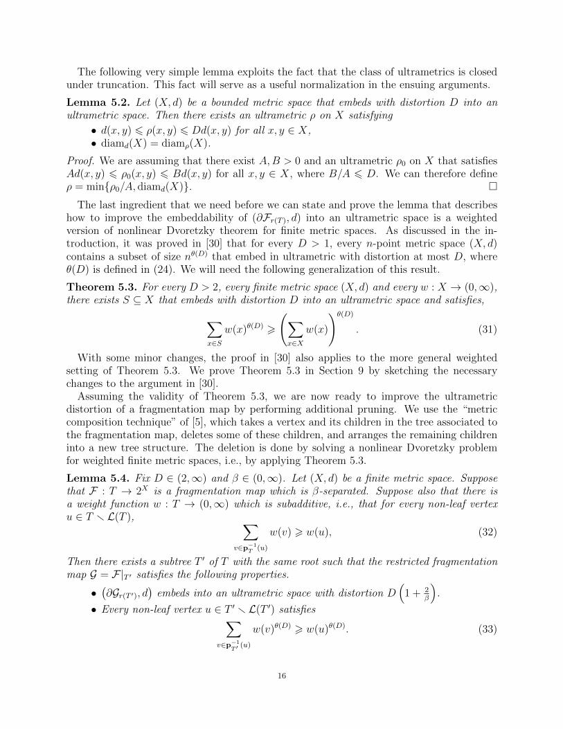
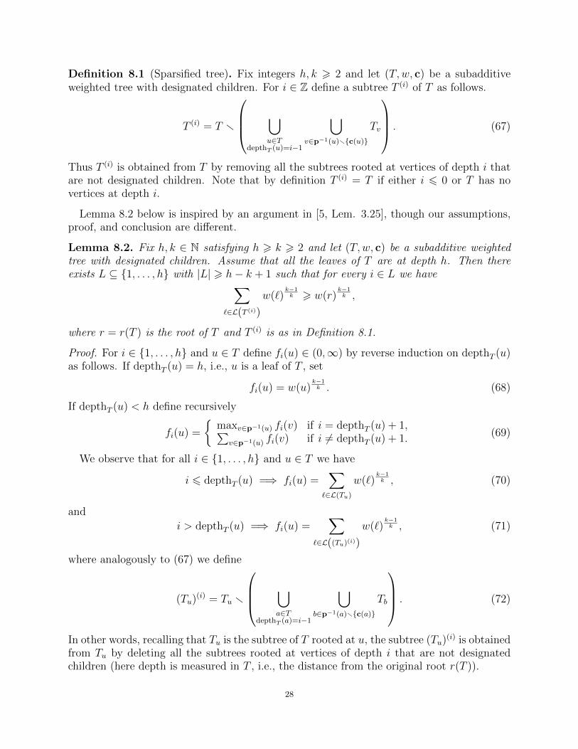
Proof. Before delving into the details of proof, the reader may want to consult Figure 1, inwhich the strategy of the proof is illustrated.

Figure 1. A schematic illustration of the proof of Lemma 5.4. Thefirst figure from the left depicts three levels of the fragmentation map,the middle level being separated. In the second figure from the leftwe consider a certain induced metric (see (34)) on the clusters in themiddle level. Due to the separation property, this metric approximatesthe actual distances between points in different clusters. In the thirdfigure from the left we have applied the weighted finite Dvoretzky the-orem, i.e., Theorem 5.3, to the middle level clusters, thus obtaining anappropriately large subset of clusters on which the induced metric isapproximately an ultrametric. The rightmost figure describes the treerepresentation of this new ultrametric.

For every vertex u ∈ T rL(T ) let Cu = p−1T (u) be the set of children of u in T . Let du be

a metric defined on Cu as follows

du(x, y) =

{diamd ((∂Fx) ∪ (∂Fy)) if x 6= y,0 if x = y.

(34)

The validity of the triangle inequality for du is immediate to verify. By the definition of θ(D)there exists a subset Su ⊆ Cu such that

∑x∈Su

w(x)θ(D)(31)

>

(∑x∈Cu

w(x)

)θ(D)(32)

> w(u)θ(D). (35)

and (Su, du) embeds with distortion D into an ultrametric space. By Lemma 5.2 there existsan ultrametric ρu on Su such that every x, y ∈ Su satisfy

du(x, y) 6 ρu(x, y) 6 min{

diamdu(Su), Ddu(x, y)

}(34)

6 min

{diamd

( ⋃x∈Su

∂Fx

), Ddu(x, y)

}. (36)

The subtree T ′ ⊆ T is now defined inductively in a top-down fashion as follows: declarer(T ) ∈ T ′ and if u ∈ T is a non-leaf vertex that was already declared to be in T ′, add thevertices in Su to T ′ as well. Inequality (33) follows from (35). It remains to prove that(∂Gr(T ′), d

)embeds into an ultrametric space with distortion D (1 + 2/β). To this end fix

p, q ∈ ∂Gr(T ′) and choose the corresponding a, b ∈ L(T ′) such that Ga = {p} and Gb = {q}.Let u = lcaT ′(a, b) = lcaT (a, b) and choose x, y ∈ Su that are weak ancestors of a and b,

17

respectively. Define ρ(p, q) = ρu(x, y). Now,

d(p, q) = d(Ga,Gb) 6 diamd ((∂Fx) ∪ (∂Fy))(34)= du(x, y)

(36)

6 ρu(x, y) = ρ(p, q).

The corresponding lower bound on d(p, q) is proved as follows, using the assumption thatthe fragmentation map F is β-separated.

ρ(p, q)

D

(36)

6 du(x, y)(34)

6 diamd (∂Fx) + diamd (∂Fy) + d (∂Fx, ∂Fy)(30)

6

(1 +

2

β

)d(p, q).

We now argue that ρ is an ultrametric on ∂Gr(T ′). This is where we will use the truncation

in (36), i.e., that for all u ∈ T r L(T ) we have diamρu(Su) 6 diamd

(⋃x∈Su ∂Fx

). Take

p1, p2, p3 ∈ ∂Gr(T ′) and choose the corresponding a1, a2, a3 ∈ L(T ′) such that Gai = {pi} fori ∈ {1, 2, 3}. By relabeling the points if necessary, we may assume that u = lcaT (a1, a2) is aweak descendant of v = lcaT (a2, a3). If u = v take x1, x2, x3 ∈ Su that are weak ancestors ofa1, a2, a3, respectively. Since ρu is an ultrametric, it follows that

ρ(p1, p2) = ρu(x1, x2) 6 max {ρu(x1, x3), ρu(x3, x2)} = max {ρu(p1, p3), ρu(p3, p2)} .If, on the other hand, u is a proper descendant of v then choose x1, x2 ∈ Su that areweak ancestors of a1, a2 (respectively), and choose s, t ∈ Sv that are weak ancestors of u, a3

(respectively). Then,

ρ(p1, p2) = ρu(x, y)(36)

6 diamd

( ⋃w∈Su

∂Fw

)6 diamd(∂Fs)

6 diamd ((∂Fs) ∪ (∂Ft))(34)= dv(s, t)

(36)

6 ρv(s, t) = ρ(p1, p3) = ρ(p2, p3).

This establishes the ultratriangle inequality for ρ, completing the proof of Lemma 5.4. �

The next lemma establishes the existence of an intermediate fragmentation map withuseful geometric properties; its proof is deferred to Section 6.

Lemma 5.5. Fix τ ∈ (0, 1/3) and integers m,h, k > 2 with h > 2k2. Let (X, d, µ) be a finitemetric measure space of diameter 1. Then there exists a fragmentation map F : T → 2X

with the following properties.

{1} All the leaves of the tree T are at depth mh.{2} For every u ∈ T we have

diam(Fu) 6 τdepthT (u). (37)

{3} Denote by R ⊆ T the set of vertices at depths which are integer multiples of h. Thenfor every non-leaf u ∈ R,∑

v∈DT (u,R)

µ (Fv)(1− 1k)

2

> µ (Fu)(1− 1k)

2

. (38)

Recall that DT (·, ·) is given in Definition 3.3.{4} There is a subset S ⊆ T containing the root of T such that R and S are “alternating” in

the following sense. For every u, v ∈ R such that depthT (v) = depthT (u) + h and v isa descendant of u, there is one and only one w ∈ S such that w lies on the path joiningu and v and depthT (u) < depthT (w) 6 depthT (v).

18

{5} The vertices of S are 1−3τ2τ

-separated (recall Definition 5.1).

{6} F is(

21−3τ

τ−2h, τ−1)-lacunary (recall Definition 3.7).

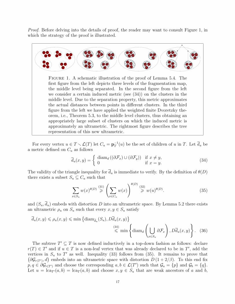
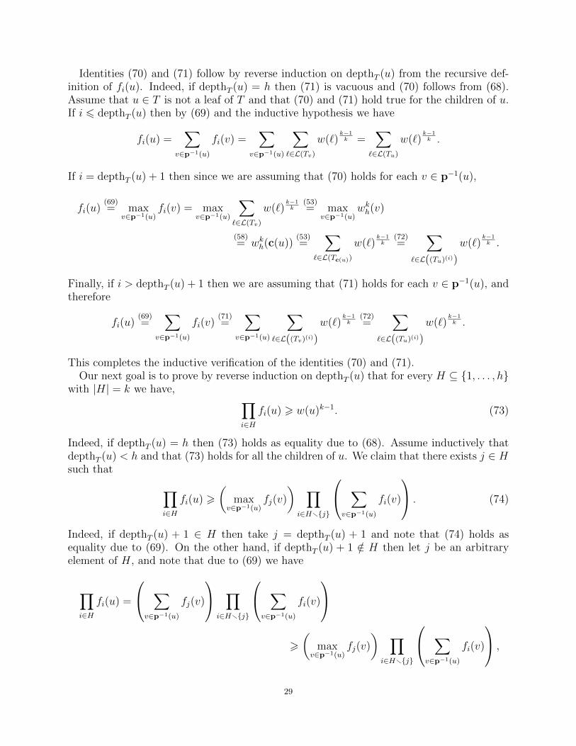
The vertices of the subset R ⊆ T of Lemma 5.5 satisfy an inductive inequality (38) on themeasures of their images that will allow us to (eventually) deduce the covering property (27)of Lemma 4.3. Figure 2 contains a schematic depiction of the fact that the levels of R andS alternate.

h

2h

3h

4hR

S

R

S

R

S

RS

R, S 0

Figure 2. A schematic depiction of the tree T corresponding to thefragmentation map F of Lemma 5.5. The vertices of R are on thedotted lines. The vertices of S are on the curved solid lines. On everyroot-leaf path in T the vertices in R and S alternate.

We are now in position to prove Lemma 4.3 using Lemma 5.4 and assuming the validityof Lemma 5.5 (recall that Lemma 5.5 will be proved in Section 6).

Proof of Lemma 4.3. Let k, τ be as in Lemma 4.3. Denote h = 2k2 and fix m ∈ N satisfying

minx,y∈Xx 6=y

d(x, y) > τ (m−2)h+1. (39)

Apply Lemma 5.5 with the parameters τ,m, h, k as above, obtaining a fragmentation mapF : T 1 → 2X with corresponding subsets S,R ⊆ T 1. Let T 2 be the tree induced by T 1

on S, i.e., join u, v ∈ S by an edge of T 2 if u is an ancestor of v in T 1 and any w ∈ Sthat is an ancestor of v in T 1 is a weak ancestor of u. This is the same as the requirementv ∈ DT 1(u, S). Let S : T 2 → 2X be the fragmentation map obtained by restricting F to S.To check that S is indeed a fragmentation map we need to verify that if u ∈ L(T 2) thenFu is a singleton. To see this let v = pT 2(u) be the parent in T 2 of u. Since all the leavesof T are at depth mh, we have depthT 1(v) > (m − 2)h + 1. Using (37) we deduce thatdiam(Fu) 6 diam(Fv) 6 τ (m−2)h+1, implying that Su and Sv are both singletons due to (39).

Since by Lemma 5.5 we know that the vertices in S are 1−3τ2τ

-separated in the fragmentation

map F , it follows that the fragmentation map S is 1−3τ2τ

-separated. Lemma 5.5 also ensures

that F is(

21−3τ

τ−2h, τ−1)-lacunary. This implies that S is

(2

1−3ττ−2h, τ−2h

)-lacunary. Indeed,

due to Lemma 5.5 we know that if u ∈ S and v ∈ DT 1(u, S) is a child of u in T 2 thendepthT 1(v) 6 depthT 1(u) + 2h − 1. This implies that if q, u ∈ S are such that u is a

19

weak descendant of q in T 2 then depthT 1(u) − depthT 1(q) 6 2h (depthT 2(u)− depthT 2(q)).Hence, if v, w ∈ DT 1(u, S) are distinct children of u in T 2, choose distinct x, y ∈ T 1 thatare children of u in T 1 and weak ancestors of v, w (respectively), and use the fact that F is(

21−3τ

τ−2h, τ−1)-lacunary to deduce that

diamd(Sq) = diamd(Fq) 62τ−2h

1− 3τ· τ−(depthT1 (u)−depthT1 (q))d (∂Fx, ∂Fy)

62τ−2h

1− 3τ· τ−2h(depthT2 (u)−depthT2 (q))d (∂Sx, ∂Sy) .

Define wR : R→ (0,∞) by top-down induction as follows. Set

wR(r) = µ(X)(1− 1k)

2

, (40)

where r is the root of T 1. If u ∈ R is not a leaf and v ∈ DT 1(u,R) then define

wR(v) =wR(u)∑

z∈DT1 (u,R) µ(Fz)(1− 1k)

2 · µ(Fv)(1− 1k)

2

. (41)

Thus for every non-leaf u ∈ R we have

wR(u) =∑

v∈DT1 (u,R)

wR(v). (42)

Moreover, it follows from the recursive definition (41) combined with (38) that

∀ u ∈ R, wR(u) 6 µ(Fu)(1− 1k)

2

. (43)

Recalling the notation D∗T (x,A) as given in (14), by summing (42) we see that for allu ∈ S r L(T 2) we have ∑

x∈D∗T1 (u,R)

∑y∈DT1 (x,R)

wR(y) =∑

x∈D∗T1 (u,R)

wR(x). (44)

Notice that ⋃x∈D∗

T1 (u,R)

DT 1(x,R) =⋃

v∈DT1 (u,S)

D∗T 1(v,R), (45)

where the unions on both sides of (45) are disjoint. Hence,∑x∈D∗

T1 (u,R)

wR(x)(44)∧(45)

=∑

v∈DT1 (u,S)

∑z∈D∗

T1 (v,R)

wR(z). (46)

Define wS : S → (0,∞) by

wS(u) =∑

z∈D∗T1 (u,R)

wR(z). (47)

Then for all u ∈ S r L(T 2) we have∑v∈p−1

T2 (u)

wS(v) =∑

v∈DT1 (u,S)

wS(v)(46)∧(47)

=∑

x∈D∗T1 (u,R)

wR(x)(47)= wS(u).

20

This establishes condition (32) of Lemma 5.4 for the weighting wS of T 2. Before applyingLemma 5.4 we record one more useful fact about wS. Recall that for u ∈ S the vertex pT 2(u)is r if u = r, and otherwise it is the first proper ancestor of u in T 1 which is in S. Takeu′ ∈ D∗T 1(pT 2(u), R) which is a weak ancestor of u in T 1. Then FpT2 (u) ⊇ Fu′ , and therefore

µ(FpT2 (u)

)(1− 1k)

2

> µ (Fu′)(1− 1k)

2 (43)

> wR(u′)

(42)=

∑x∈DT1 (u′,R)

wR(x) =∑

x∈D∗T1 (u,R)

wR(x)(47)= wS(u). (48)

Apply Lemma 5.4 to S : T 2 → 2X and wS : T 2 → (0,∞), with β = (1− 3τ)/(2τ) and theparameter D of Lemma 5.4 replaced by D/(1 + 2/β) = D(1 − 3τ)/(1 + τ). Note that ourassumption τ < (D−2)/(3D+2) guarantees that this new value of D is bigger than 2, so weare indeed allowed to use Lemma 5.4. We therefore obtain a subtree T ⊆ T 2 with the sameroot, such that the restricted fragmentation map G = S|T satisfies the following properties.

• (∂Gr(T ), d) embeds into an ultrametric space with distortion D.• Every non-leaf vertex u ∈ T r L(T ) satisfies∑

v∈p−1T (u)

wS(v)θ(1−3τ1+τ

D)(33)

> wS(u)θ(1−3τ1+τ

D). (49)

Let G ⊆ T be a cut-set of T . Define G0 to be a subset of G which is still a cut-setand is minimal with respect to inclusion. Assume inductively that we defined a cut-set Gi

of T which is minimal with respect to inclusion. Let v ∈ Gi be such that depthT (v) ismaximal. Let u = pT (v). By the maximality of depthT (v), since Gi is a minimal cut-set ofT we necessarily have p−1

T (u) ⊆ Gi, i.e., all the siblings of v in T are also in Gi. Note thatG′i = (Gi ∪ {u}) r p−1

T (u) is also a cut-set of T , so let Gi+1 be a subset of G′i which is still acut-set of T and is minimal with respect to inclusion. Then,∑

v∈Gi

wS(v)θ(1−3τ1+τ

D) =∑

v∈Girp−1T (u)

wS(v)θ(1−3τ1+τ

D) +∑

v∈p−1T (u)

wS(v)θ(1−3τ1+τ

D)

(49)

>∑v∈G′i

wS(v)θ(1−3τ1+τ

D) >∑

v∈Gi+1

wS(v)θ(1−3τ1+τ

D). (50)

After finitely many iterations of the above process we will arrive at Gj = {r}. By concate-nating the inequalities (50) we see that∑v∈G

wS(v)θ(1−3τ1+τ

D) >∑v∈G0

wS(v)θ(1−3τ1+τ

D) > wS(r)θ(1−3τ1+τ

D) (40)∧(47)= µ(X)(1− 1

k)2θ( 1−3τ

1+τD). (51)

The desired inequality (27) follows from (51) and (48). Since S is 1−3τ2τ

-separated and(2

1−3ττ−4k2 , τ−4k2

)-lacunary (recall that h = 2k2), the same holds true for G since it is

the restriction of S to the subtree of T 2. �

Remark 5.6. In Theorem 1.5, if one is willing to settle for ultrametric distortion eO(1/ε2),instead of the asymptotically optimal O(1/ε) distortion, then it is possible to simplify

21

Lemma 4.3 and its proof. In particular, there is no need to apply Lemma 5.4, and con-sequently also Theorem 5.3. Thus one can use the fragmentation map S introduced inthe proof of Lemma 4.3 as the fragmentation map produced by Lemma 4.3. Since S is(

21−3τ

τ−4k2 , τ−4k2)

-lacunary, Lemma 3.8 implies that (∂Sr(S), d) embeds in an ultrametric

space with distortion 21−3τ

τ−4k2 = eO(1/ε2). It is possible to further simplify the proof of thecut-set inequality (27) in the proof of Lemma 4.3 by considering a different fragmentationmap R instead of S, defined as follows. Consider the tree T 3 induced by T 1 on R, and thefragmentation map R : T 3 → 2X obtained by restricting F to T 3. Like S, the fragmentation

map R is(

21−3τ

τ−4k2 , τ−4k2)

-lacunary, and the proof of (27) for R can now be performed by

only using the weight function wR, without the need to consider wS. Unlike S, the fragmen-tation map R is not separated, and therefore cannot be used with Lemma 5.4. However, forthe above simplified argument, Lemma 5.4 and the separation property are not needed.

6. An intermediate fragmentation map: proof of Lemma 5.5

Here we prove Lemma 5.5. The proof uses two building blocks: Lemma 6.2, which con-structs an initial partition map, and Lemma 6.5, which prunes a given weighted rooted tree.The basic idea of the proof Lemma 5.5 can be described as follows. Lemma 6.2 constructs aninitial partition map together with a “designated child” for every non leaf vertex. The desig-nated children have, roughly speaking, the largest weight among their siblings, and they arealso pairwise separated. The pruning step of Lemma 6.5 can now focus on the combinatorialstructure of the partition map, pruning the associated tree so as to keep at some levels onlythe designated children of the level above. This guarantees the separation property as wellas the desired estimate (38).

The exact notion of “size” used to choose designated children is tailored to be compatiblewith the ensuing pruning step, and is the content of the following definition. Observe thatany fragmentation map F : T → 2X induces a weighting w : T → (0,∞) of the vertices of Tgiven by w(u) = µ(Fu). For our purpose, we will need a modified version of it, described inthe following definition.

Definition 6.1 (Modified weight function). Fix integers h, k > 2 and let T be a finitegraph-theoretical rooted tree, all of whose leaves are at the same depth, which is divisibleby h. Assume that we are given w : T → (0,∞). Define a new function wkh : T → (0,∞) asfollows. If u ∈ L(T ) then

wkh(u) = w(u)k−1k .

Continue defining wkh(u) by reverse induction on depthT (u) as follows.

wkh(u) =

{w(u)

k−1k if h | depthT (u),∑

v∈p−1(u) wkh(v) if h - depthT (u).

(52)

Equivalently, if u ∈ T and (j − 1)h < depthT (u) 6 jh for some integer j then

wkh(u) =∑v∈Tu

depthT (v)=jh

w(v)k−1k . (53)

22

Lemma 6.2. Let (X, d, µ) be a finite metric measure space of diameter 1 and τ ∈ (0, 1/3).For every triple of integers m,h, k > 2 there exists a fragmentation map F : T → 2X withthe following properties.

• All the leaves of the tree T are at depth mh.• F is a partition map, i.e., ∂Fr(T ) = X.• For every u ∈ T we have

diam(Fu) 6 τdepthT (u). (54)

• Every non-leaf vertex u ∈ T rL(T ) has a “designated child” c(u) ∈ p−1(u) such that

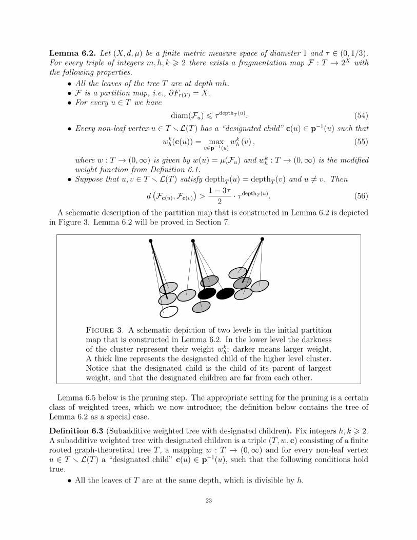
wkh(c(u)) = maxv∈p−1(u)

wkh (v) , (55)

where w : T → (0,∞) is given by w(u) = µ(Fu) and wkh : T → (0,∞) is the modifiedweight function from Definition 6.1.• Suppose that u, v ∈ T r L(T ) satisfy depthT (u) = depthT (v) and u 6= v. Then

d(Fc(u),Fc(v)

)>

1− 3τ

2· τdepthT (u). (56)

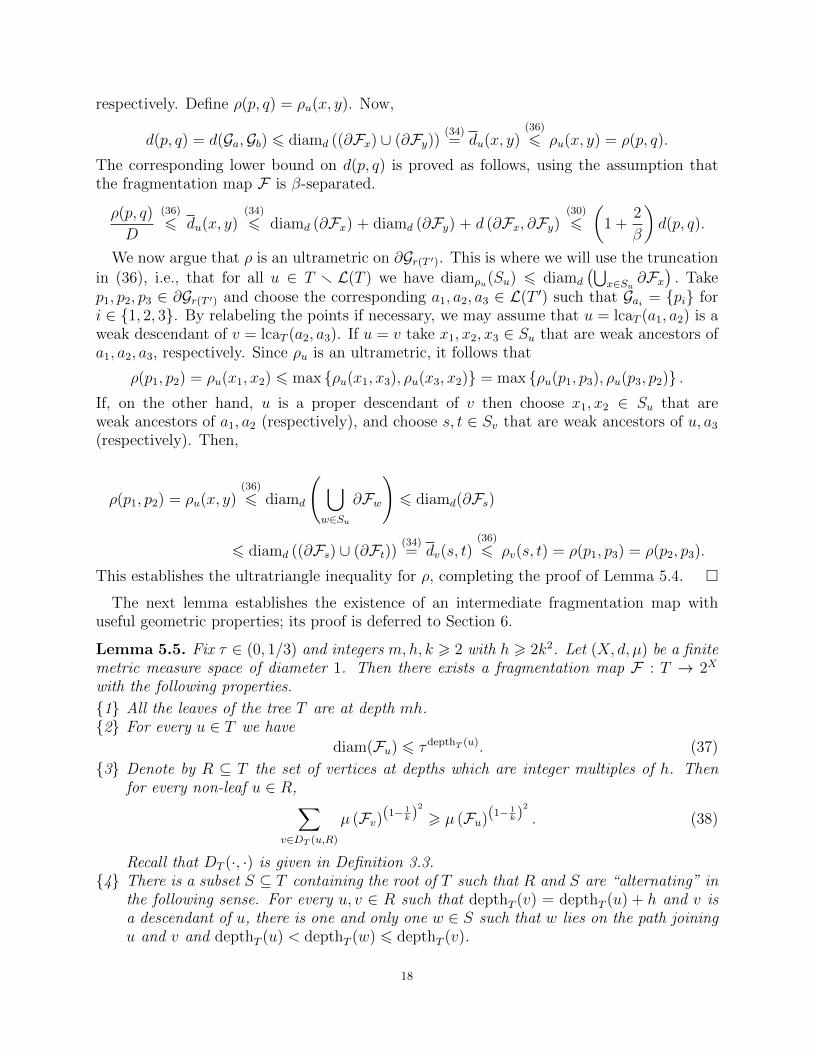
A schematic description of the partition map that is constructed in Lemma 6.2 is depictedin Figure 3. Lemma 6.2 will be proved in Section 7.

Figure 3. A schematic depiction of two levels in the initial partitionmap that is constructed in Lemma 6.2. In the lower level the darknessof the cluster represent their weight wkh; darker means larger weight.A thick line represents the designated child of the higher level cluster.Notice that the designated child is the child of its parent of largestweight, and that the designated children are far from each other.

Lemma 6.5 below is the pruning step. The appropriate setting for the pruning is a certainclass of weighted trees, which we now introduce; the definition below contains the tree ofLemma 6.2 as a special case.

Definition 6.3 (Subadditive weighted tree with designated children). Fix integers h, k > 2.A subadditive weighted tree with designated children is a triple (T,w, c) consisting of a finiterooted graph-theoretical tree T , a mapping w : T → (0,∞) and for every non-leaf vertexu ∈ T r L(T ) a “designated child” c(u) ∈ p−1(u), such that the following conditions holdtrue.

• All the leaves of T are at the same depth, which is divisible by h.

23

• For every non-leaf vertex u ∈ T r L(T ),

w(u) 6∑

v∈p−1(u)

w(v). (57)

• For every non-leaf vertex u ∈ T r L(T ),

wkh(c(u)) = maxv∈p−1(u)

wkh(v), (58)

where wkh : T → (0,∞) is the modified weight function of Definition 6.1.

Definition 6.4 (Subtree sparsified at a subset). Fix two integers h, k > 2 and let let (T,w, c)be a subadditive weighted tree with designated children (recall Definition 6.3). Let T ′ be asubtree of T (see Definition 3.2) and S ⊆ T ′. We say that the subtree T ′ is sparsified at S ifevery v ∈ S is a designated child and has no siblings in T ′. For the purpose of this definitionwe declare the root r(T ) to be a designated child, i.e., we allow r(T ) ∈ S. Thus v ∈ T is adesignated child if it is either the root of T or c(p(v)) = v.

Lemma 6.5. Fix two integers h, k > 2 with h > 2k2. Let (T,w, c) be a subadditive weightedtree with designated children as in Definition 6.3 (thus all the leaves of T are at the samedepth, which is divisible by h, and the designated child map c satisfies (58)). Then thereexists a subtree T ′ of T with the same root as T , and two subsets R, S ⊆ T ′, both containingthe root of T ′, with the following properties:

• For any non-leaf u ∈ T ′ we have c(u) ∈ T ′.• R = {v ∈ T ′ : h | depthT (v)}.• For any non-leaf vertex u ∈ R,∑

v∈DT ′ (u,R)

w(v)(1− 1k)

2

> w(u)(1− 1k)

2

. (59)

Recall that DT ′(·, ·) is given in Definition 3.3.• For every u, v ∈ R such that depthT (v) = depthT (u) + h and v is a descendant of u,

there is one and only one w ∈ S such that w lies on the path joining u and v anddepthT (u) < depthT (w) 6 depthT (v).• For any u ∈ T ′ such that DT ′(u, S) 6= ∅, all the vertices of DT ′(u, S) are at the same

depth in T ′u, which is an integer between 1 and 2h.• T ′ is sparsified at the subset S.

Lemma 6.5 will be proved in Section 8. Assuming the validity of Lemma 6.5, as well asthe validity of Lemma 6.2 (which will be proved is Section 7), we are now in position todeduce Lemma 5.5.

Proof of Lemma 5.5. Let F0 : T 0 → 2X be the partition map of Lemma 6.2, constructedwith parameters m,h, k, and having the associated designated child map c from Lemma 6.2.Let T be the tree obtained by applying Lemma 6.5 to (T 0, w, c), where w : T 0 → (0,∞) isgiven by w(v) = µ(F0

v ). Define a fragmentation map F : T → 2X by F = F0|T , i.e., byrestricting F0 to the subtree T . Properties {1}, {2} are satisfied by F0 due to Lemma 6.2,and therefore they are also satisfied by F since T has the same root as T 0. Properties {3},{4}, are part of the conclusion of Lemma 6.5. It remains to prove properties {5} and {6}.

24

Assume that u ∈ S. Take y ∈(∂Fr(T )

)r (∂Fu). In order to prove property {5} it suffices

to show that d(y,Fu) > 1−3τ2τ

diam(Fu). By property {4} it follows that u = c(p(u)). Letw = lcaT (u, y) and take u′, y′ ∈ DT (w, S) such that u′ is a weak ancestor of u and y′ is aweak ancestor of y. By Lemma 6.5 we know that depthT (u′) = depthT (y′), and thereforeby conclusion (56) of Lemma 6.2 and using the fact that c(p(u′)) = u′ and c(p(y′)) = y′

(because u′, y′ ∈ S),

d (y,Fu) > d (Fy′ ,Fu′) >1− 3τ

2τdepthT (u′)−1 >

1− 3τ

2ττdepthT (u)

(37)

>1− 3τ

2τdiam(Fu).

It remains to prove property {6}. Take q ∈ T and let u ∈ T be a weak descendent of qthat has at least two children in T , i.e., v, w ∈ p−1(u) ∩ T , v 6= w. Our goal is to show that

diam (Fq) 62τ−2h

1− 3τ· τdepthT (q)−depthT (u) · d (∂Fv, ∂Fw) . (60)

Since v and w are siblings in T we know by {4} that {v, w} ∩ S = ∅. Note that

∂Fv =⋃

y∈D(v,S)

∂Fy and ∂Fw =⋃

x∈D(w,S)

∂Fx,

and therefored (∂Fv, ∂Fw) = min

y∈D(v,S)x∈D(w,S)

d (∂Fy, ∂Fx) . (61)

Note that since {v, w} ∩ S = ∅ we have D(v, S) ∪ D(w, S) ⊆ D(u, S). By Lemma 6.5 itfollows that all the vertices in D(v, S) ∪ D(w, S) are at the same depth in T . Denote thisdepth by `. Due to Lemma 6.5 we know that ` 6 depthT (u) + 2h. By conclusion (56) ofLemma 6.2 we deduce that for all y ∈ D(v, S) and x ∈ D(w, S) we have

d (∂Fy, ∂Fx) > d (Fy,Fx) = d(Fc(p(y)),Fc(p(x))

)>

1− 3τ

2τ ` >

1− 3τ

2τdepthT (u)+2h. (62)

Now, the desired inequality (60) is proved as follows.

d (∂Fv, ∂Fw)(61)∧(62)>

1− 3τ

2τdepthT (u)+2h

(37)

>1− 3τ

2τdepthT (u)−depthT (q)+2h diam(Fq). �

7. The initial fragmentation map: proof of Lemma 6.2

Proof of Lemma 6.2. The construction of the initial fragmentation map will be in a bottom-up fashion: the tree T will be decomposed as a disjoint union on “levels” V0, V1, . . . , Vmh,where Vi are the vertices at depth i. We will construct these levels Vi and the mappingsF : Vi → 2X and wkh : Vi → (0,∞) by reverse induction on i, and describe inductively foreach v ∈ Vi+1 its parent u ∈ Vi, as well as the designated child c(u). At the end of thisconstruction V0 will consist of a single vertex, the root of T .

Define `mh = |X| and write X = {x1, . . . , x`mh}. The initial level Vmh consists of the leaves

of T , and it is defined to be Vmh = {vmhj }`mhj=1. For all j ∈ {1, . . . , `mh} we also set

Fvmhj = {xj} and wkh(vmhj ) = w(xj)

k−1k = µ({xj})

k−1k .

Assume inductively that for i ∈ {1, . . . ,mh− 1} we have already defined

Vi+1 ={vi+1

1 , vi+12 , . . . , vi+1

`i+1

},

25

and the mappings F : Vi+1 → 2X and wkh : Vi+1 → (0,∞).Choose j1 ∈ {1, . . . , `i+1} such that

wkh(vi+1j1

)= max

j∈{1,...,`i+1}wkh(vi+1j

).

Define

Ai1 =

{s ∈ {1, . . . , `i+1} : d

(Fvi+1

j1

,Fvi+1s

)6

1− 3τ

2τ i}.

Create a new vertex vi1 ∈ Vi and define

Fvi1 =⋃s∈Ai1

Fvi+1s.

Also, declare the vertices {vi+1s }s∈Ai1 ⊆ Vi+1 to be the children of vi1, and in accordance

with (52) define

wkh(vi1)

=

{w (vi1)

k−1k if h | i,∑

s∈Ai1wkh (vi+1

s ) if h - i.Finally, set

c(vi1)

= vi+1j1.

Continuing inductively, assume that we have defined vi1, vi2, . . . , v

iz ∈ Vi, together with

nonempty disjoint sets

Ai1, . . . , Aiz ⊆ {1, . . . , `i+1}.

If⋃zt=1 A

it = {1, . . . , `i+1} then define `i = z and Vi = {vi1, vi2, . . . , viz}. Otherwise, choose

jz+1 ∈ {1, . . . , `i+1}r⋃zt=1A

it such that

wkh

(vi+1jz+1

)= max

j∈{1,...,`i+1}r⋃zt=1 A

it

wkh(vi+1j

), (63)

and define

Aiz+1 =

{s ∈ {1, . . . , `i+1}r

z⋃t=1

Ait : d(Fvi+1

jz+1

,Fvi+1s

)6

1− 3τ

2τ i

}. (64)

Create a new vertex viz+1 ∈ Vi and define

Fviz+1=

⋃s∈Aiz+1

Fvi+1s. (65)

Also, declare the vertices {vi+1s }s∈Aiz+1

⊆ Vi+1 to be the children of viz+1 and define

wkh(viz+1

)=

{w(viz+1

) k−1k if k | i,∑

s∈Aiz+1wkh (vi+1

s ) if k - i.

Finally, set

c(viz+1

)= vi+1

jz+1. (66)

The above recursive procedure must terminate, yielding the level i set Vi. We then proceedinductively until the set V1 has been defined. We conclude by defining V0 to be a single newvertex r(T ) (the root) with all the vertices in V1 its children. The designated child of the

26

root, c(r(T )), is chosen to be a vertex u ∈ V1 such that wkh (u) = maxv∈V1 wkh (v). We also

set Fr(T ) = X and wkh(r(T )) = µ(X)k−1k .

The resulting fragmentation map F : T → 2X is by definition a partition map, sinceF(Vmh) = F(L(T )) = X. Also, the construction above guarantees the validity of (55) dueto (63) and (66).

We shall now prove (54) by reverse induction on depthT (u). If depthT (u) = mh thendiam(Fu) = 0 and there is nothing to prove. Assuming the validity of (54) wheneverdepthT (u) = i + 1, suppose that depthT (u) = i and moreover that u = viz+1 in the aboveconstruction. By virtue of (64) and (65) we know that

diam (Fu) = diam(Fviz+1

)6 3 max

s∈Aiz+1

diam(F i+1vs

)+ 2

1− 3τ

2τ i 6 3τ i+1 + (1− 3τ)τ i = τ i.

Since (54) is also valid for i = 0 (because diam(X) = 1), this concludes the proof of (54).It remains to prove (56). Since we are assuming that u 6= v are non-leaf vertices and

depthT (u) = depthT (v), we may write u = vis and v = vit for some i ∈ {1, . . . ,mh − 1} ands < t. Then by the above construction c (vis) = vi+1

js, c (vit) = vi+1

jtand

jt ∈ {1, . . . , `i+1}rt−1⋃`=1

Ai` ⊆ {1, . . . , `i+1}rs−1⋃`=1

Ai`,

yet jt /∈ Ais. The validity of (56) now follows from the definition of Ais; see (64). �

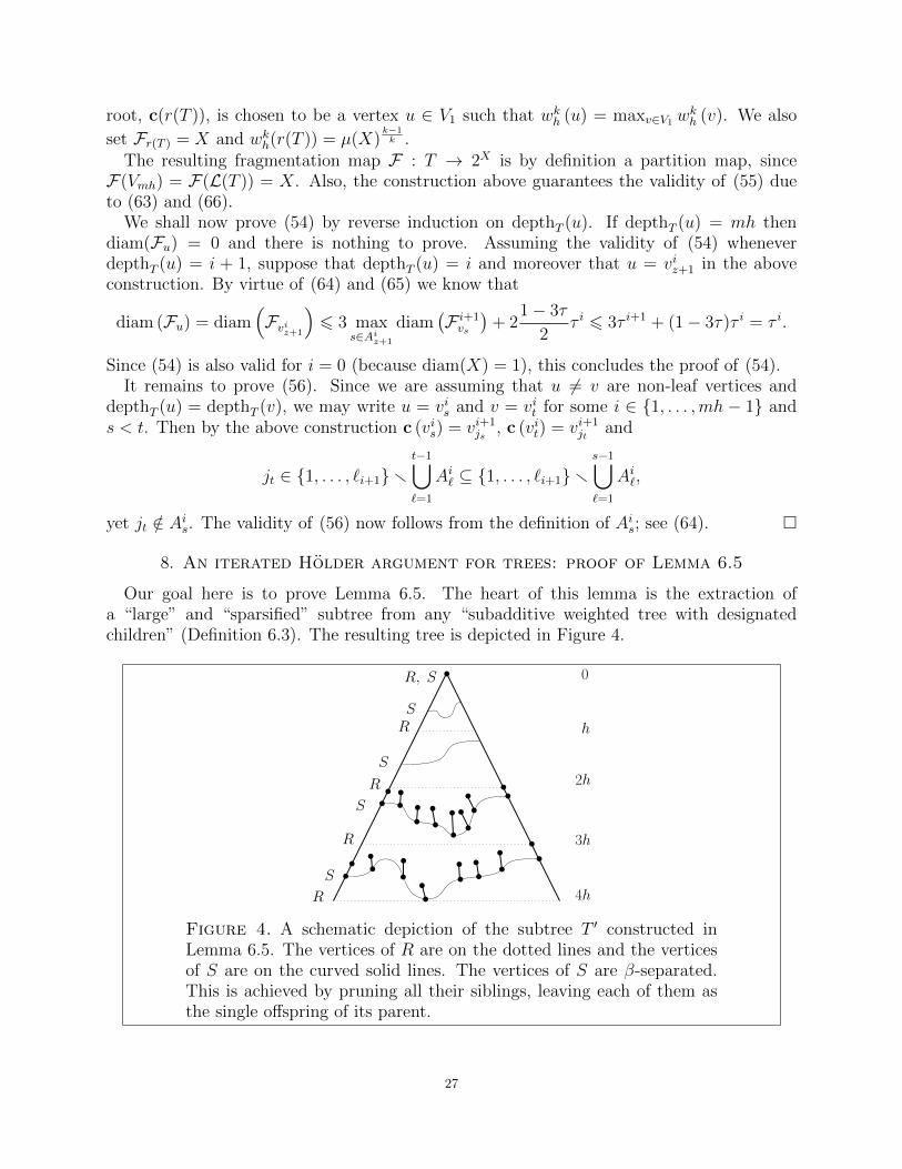
8. An iterated Holder argument for trees: proof of Lemma 6.5

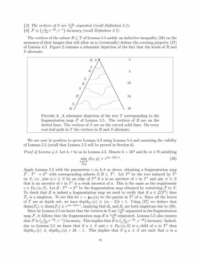
Our goal here is to prove Lemma 6.5. The heart of this lemma is the extraction ofa “large” and “sparsified” subtree from any “subadditive weighted tree with designatedchildren” (Definition 6.3). The resulting tree is depicted in Figure 4.

h

2h

3h

4hR

S

R

S

R

S

RS

R, S 0

Figure 4. A schematic depiction of the subtree T ′ constructed inLemma 6.5. The vertices of R are on the dotted lines and the verticesof S are on the curved solid lines. The vertices of S are β-separated.This is achieved by pruning all their siblings, leaving each of them asthe single offspring of its parent.

27

Definition 8.1 (Sparsified tree). Fix integers h, k > 2 and let (T,w, c) be a subadditiveweighted tree with designated children. For i ∈ Z define a subtree T (i) of T as follows.

T (i) = T r

⋃u∈T

depthT (u)=i−1

⋃v∈p−1(u)r{c(u)}

Tv

. (67)

Thus T (i) is obtained from T by removing all the subtrees rooted at vertices of depth i thatare not designated children. Note that by definition T (i) = T if either i 6 0 or T has novertices at depth i.

Lemma 8.2 below is inspired by an argument in [5, Lem. 3.25], though our assumptions,proof, and conclusion are different.

Lemma 8.2. Fix h, k ∈ N satisfying h > k > 2 and let (T,w, c) be a subadditive weightedtree with designated children. Assume that all the leaves of T are at depth h. Then thereexists L ⊆ {1, . . . , h} with |L| > h− k + 1 such that for every i ∈ L we have∑

`∈L(T (i))

w(`)k−1k > w(r)

k−1k ,

where r = r(T ) is the root of T and T (i) is as in Definition 8.1.

Proof. For i ∈ {1, . . . , h} and u ∈ T define fi(u) ∈ (0,∞) by reverse induction on depthT (u)as follows. If depthT (u) = h, i.e., u is a leaf of T , set

fi(u) = w(u)k−1k . (68)

If depthT (u) < h define recursively

fi(u) =

{maxv∈p−1(u) fi(v) if i = depthT (u) + 1,∑

v∈p−1(u) fi(v) if i 6= depthT (u) + 1.(69)

We observe that for all i ∈ {1, . . . , h} and u ∈ T we have

i 6 depthT (u) =⇒ fi(u) =∑

`∈L(Tu)

w(`)k−1k , (70)

and

i > depthT (u) =⇒ fi(u) =∑

`∈L((Tu)(i))

w(`)k−1k , (71)

where analogously to (67) we define

(Tu)(i) = Tu r

⋃a∈T

depthT (a)=i−1

⋃b∈p−1(a)r{c(a)}

Tb

. (72)

In other words, recalling that Tu is the subtree of T rooted at u, the subtree (Tu)(i) is obtained

from Tu by deleting all the subtrees rooted at vertices of depth i that are not designatedchildren (here depth is measured in T , i.e., the distance from the original root r(T )).

28

Identities (70) and (71) follow by reverse induction on depthT (u) from the recursive def-inition of fi(u). Indeed, if depthT (u) = h then (71) is vacuous and (70) follows from (68).Assume that u ∈ T is not a leaf of T and that (70) and (71) hold true for the children of u.If i 6 depthT (u) then by (69) and the inductive hypothesis we have

fi(u) =∑

v∈p−1(u)

fi(v) =∑

v∈p−1(u)

∑`∈L(Tv)

w(`)k−1k =

∑`∈L(Tu)

w(`)k−1k .

If i = depthT (u) + 1 then since we are assuming that (70) holds for each v ∈ p−1(u),

fi(u)(69)= max

v∈p−1(u)fi(v) = max

v∈p−1(u)

∑`∈L(Tv)

w(`)k−1k

(53)= max

v∈p−1(u)wkh(v)

(58)= wkh(c(u))

(53)=

∑`∈L(Tc(u))

w(`)k−1k

(72)=

∑`∈L((Tu)(i))

w(`)k−1k .

Finally, if i > depthT (u) + 1 then we are assuming that (71) holds for each v ∈ p−1(u), andtherefore

fi(u)(69)=

∑v∈p−1(u)

fi(v)(71)=

∑v∈p−1(u)

∑`∈L((Tv)(i))

w(`)k−1k

(72)=

∑`∈L((Tu)(i))

w(`)k−1k .

This completes the inductive verification of the identities (70) and (71).Our next goal is to prove by reverse induction on depthT (u) that for every H ⊆ {1, . . . , h}

with |H| = k we have, ∏i∈H

fi(u) > w(u)k−1. (73)

Indeed, if depthT (u) = h then (73) holds as equality due to (68). Assume inductively thatdepthT (u) < h and that (73) holds for all the children of u. We claim that there exists j ∈ Hsuch that ∏

i∈H

fi(u) >

(max

v∈p−1(u)fj(v)

) ∏i∈Hr{j}

∑v∈p−1(u)

fi(v)

. (74)

Indeed, if depthT (u) + 1 ∈ H then take j = depthT (u) + 1 and note that (74) holds asequality due to (69). On the other hand, if depthT (u) + 1 /∈ H then let j be an arbitraryelement of H, and note that due to (69) we have

∏i∈H

fi(u) =

∑v∈p−1(u)

fj(v)

∏i∈Hr{j}

∑v∈p−1(u)

fi(v)

>

(max

v∈p−1(u)fj(v)

) ∏i∈Hr{j}

∑v∈p−1(u)

fi(v)

,

29

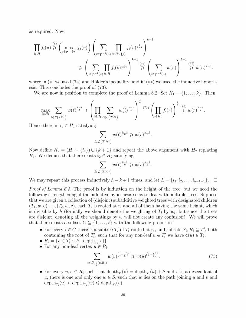
as required. Now,

∏i∈H

fi(u)(∗)>

(max

v∈p−1(u)fj(v)

) ∑v∈p−1(u)

∏i∈Hr{j}

fi(v)1

k−1

k−1

>

∑v∈p−1(u)

∏i∈H

fi(v)1

k−1

k−1

(∗∗)>

∑v∈p−1(u)

w(v)

k−1

(57)

> w(u)k−1,

where in (∗) we used (74) and Holder’s inequality, and in (∗∗) we used the inductive hypoth-esis. This concludes the proof of (73).

We are now in position to complete the proof of Lemma 8.2. Set H1 = {1, . . . , k}. Then

maxi∈H1

∑`∈L(T (i))

w(`)k−1k >

∏i∈H1

∑`∈L(T (i))

w(`)k−1k

1k

(71)=

(∏i∈H1

fi(r)

) 1k (73)

> w(r)k−1k .

Hence there is i1 ∈ H1 satisfying ∑`∈L(T (i1))

w(`)k−1k > w(r)

k−1k .

Now define H2 = (H1 r {i1}) ∪ {k + 1} and repeat the above argument with H2 replacingH1. We deduce that there exists i2 ∈ H2 satisfying∑

`∈L(T (i2))

w(`)k−1k > w(r)

k−1k .

We may repeat this process inductively h− k+ 1 times, and let L = {i1, i2, . . . , ih−k+1}. �

Proof of Lemma 6.5. The proof is by induction on the height of the tree, but we need thefollowing strengthening of the inductive hypothesis so as to deal with multiple trees. Supposethat we are given a collection of (disjoint) subadditive weighted trees with designated children(T1, w, c) . . . , (T`, w, c), each Ti is rooted at ri and all of them having the same height, whichis divisible by h (formally we should denote the weighting of Ti by wi, but since the treesare disjoint, denoting all the weightings by w will not create any confusion). We will provethat there exists a subset C ⊆ {1, . . . , `} with the following properties.

• For every i ∈ C there is a subtree T ′i of Ti rooted at ri, and subsets Si, Ri ⊆ T ′i , bothcontaining the root of T ′i , such that for any non-leaf u ∈ T ′i we have c(u) ∈ T ′i .• Ri = {v ∈ T ′i : h | depthTi(v)}.• For any non-leaf vertex u ∈ Ri,∑

v∈DT ′i(u,Ri)

w(v)(1− 1k)

2

> w(u)(1− 1k)

2

. (75)

• For every u, v ∈ Ri such that depthTi(v) = depthTi(u) + h and v is a descendant ofu, there is one and only one w ∈ Si such that w lies on the path joining u and v anddepthTi(u) < depthTi(w) 6 depthTi(v).

30

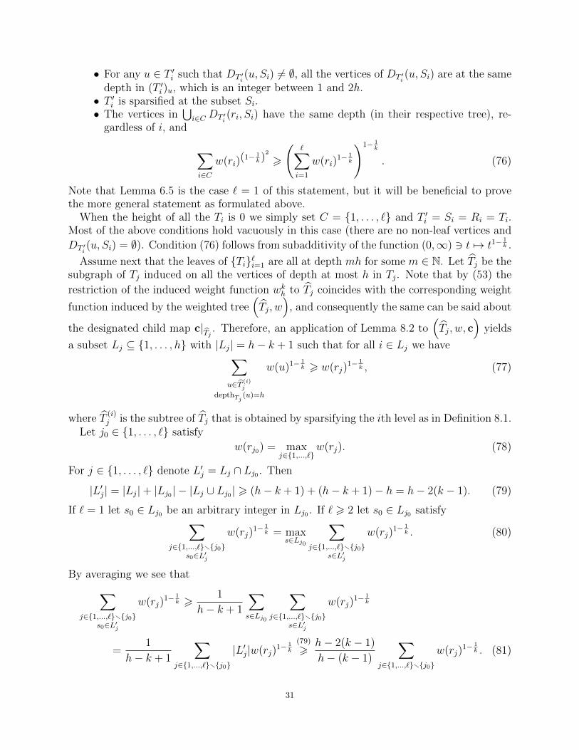
• For any u ∈ T ′i such that DT ′i(u, Si) 6= ∅, all the vertices of DT ′i

(u, Si) are at the samedepth in (T ′i )u, which is an integer between 1 and 2h.• T ′i is sparsified at the subset Si.• The vertices in

⋃i∈C DT ′i

(ri, Si) have the same depth (in their respective tree), re-gardless of i, and

∑i∈C

w(ri)(1− 1

k)2

>

(∑i=1

w(ri)1− 1

k

)1− 1k

. (76)

Note that Lemma 6.5 is the case ` = 1 of this statement, but it will be beneficial to provethe more general statement as formulated above.

When the height of all the Ti is 0 we simply set C = {1, . . . , `} and T ′i = Si = Ri = Ti.Most of the above conditions hold vacuously in this case (there are no non-leaf vertices and

DT ′i(u, Si) = ∅). Condition (76) follows from subadditivity of the function (0,∞) 3 t 7→ t1−

1k .

Assume next that the leaves of {Ti}`i=1 are all at depth mh for some m ∈ N. Let Tj be thesubgraph of Tj induced on all the vertices of depth at most h in Tj. Note that by (53) the

restriction of the induced weight function wkh to Tj coincides with the corresponding weight

function induced by the weighted tree(Tj, w

), and consequently the same can be said about

the designated child map c|Tj . Therefore, an application of Lemma 8.2 to(Tj, w, c

)yields

a subset Lj ⊆ {1, . . . , h} with |Lj| = h− k + 1 such that for all i ∈ Lj we have∑u∈T (i)

j

depthTj (u)=h

w(u)1− 1k > w(rj)

1− 1k , (77)

where T(i)j is the subtree of Tj that is obtained by sparsifying the ith level as in Definition 8.1.

Let j0 ∈ {1, . . . , `} satisfy

w(rj0) = maxj∈{1,...,`}

w(rj). (78)

For j ∈ {1, . . . , `} denote L′j = Lj ∩ Lj0 . Then

|L′j| = |Lj|+ |Lj0| − |Lj ∪ Lj0 | > (h− k + 1) + (h− k + 1)− h = h− 2(k − 1). (79)

If ` = 1 let s0 ∈ Lj0 be an arbitrary integer in Lj0 . If ` > 2 let s0 ∈ Lj0 satisfy∑j∈{1,...,`}r{j0}

s0∈L′j

w(rj)1− 1

k = maxs∈Lj0

∑j∈{1,...,`}r{j0}

s∈L′j

w(rj)1− 1

k . (80)

By averaging we see that∑j∈{1,...,`}r{j0}

s0∈L′j

w(rj)1− 1

k >1

h− k + 1

∑s∈Lj0

∑j∈{1,...,`}r{j0}

s∈L′j

w(rj)1− 1

k

=1

h− k + 1

∑j∈{1,...,`}r{j0}

|L′j|w(rj)1− 1

k

(79)

>h− 2(k − 1)

h− (k − 1)

∑j∈{1,...,`}r{j0}

w(rj)1− 1

k . (81)

31

Now defineC = {j ∈ {1, . . . , `} : s0 ∈ Lj} . (82)

We know that j0 ∈ C, since by construction s0 ∈ Lj0 . By (79) we have L′j 6= ∅ for everyj ∈ {1, . . . , `}. Therefore (80) implies that if ` > 2 then |C| > 2. Since (76) is trivial when` = 1, we will now prove (76) assuming ` > 2. By the choice of j0 in (78) we know that forall j ∈ {1, . . . , `}r {j0} we have

w (rj)1− 1

k 61

2

∑i=1

w(ri)1− 1

k . (83)

This implies that for all j ∈ {1, . . . , `}r {j0},

w(rj)(1− 1

k)2

>h− (k − 1)

h− 2(k − 1)· w(rj)

1− 1k(∑`

i=1w(ri)1− 1

k

) 1k

. (84)

To check (84) note that it is equivalent to the inequality

h− (k − 1)

h− 2(k − 1)

(w(rj)

1− 1k∑`

i=1 w(ri)1− 1

k

) 1k

6 1.

By (83) and the fact that h > 2k2, it suffices to show that (2k2−k+1)/(2k2−2k+2) 6 21/k.Since 21/k > 1 + 1/(2k) it suffices to check that 2k(2k2 − k + 1) 6 (2k + 1)(2k2 − 2k + 2),which is immediate to verify.

Having established (84), we proceed as follows.∑j∈C

w(rj)(1− 1

k)2

=w(rj0)

1− 1k

w(rj0)(1− 1

k)1k

+∑

j∈Cr{j0}

w(rj)(1− 1

k)2

(84)

>w(rj0)

1− 1k(∑`

i=1 w(ri)1− 1

k

) 1k

+h− (k − 1)

h− 2(k − 1)·∑

j∈Cr{j0}w(rj)1− 1

k(∑`i=1w(ri)

1− 1k

) 1k

(81)∧(82)

>w(rj0)

1− 1k(∑`

i=1 w(ri)1− 1

k

) 1k

+

∑j∈{1,...,`}r{j0}w(rj)

1− 1k(∑`

i=1 w(ri)1− 1

k

) 1k

=

(∑i=1

w(ri)1− 1

k

)1− 1k

,

completing the proof of (76).We can now complete the proof of Lemma 6.5 by applying the inductive hypothesis. For

every j ∈ C let uj1, uj2, . . . , u

j`j

be the leaves of the tree T(s0)j , i.e., the subtree of Tj that

was sparsified at level s0. Consider the subtrees of Tj that are rooted at uj1, uj2, . . . , u

j`j

, i.e.,

(Tj)uj1, (Tj)uj2

, . . . , (Tj)uj`j. By the inductive hypothesis applied to these trees there exists a

subset Cj ⊆ {1, . . . , `j} such that for each i ∈ Cj there is a subtree (Tj)′uji

of (Tj)ujiand

subsets Sji, Rji ⊆ (Tj)′uji

that satisfy the inductive hypotheses.

32

Denote for j ∈ C,

T ′j =

⋃i∈Cj

(Tj)′uji

⋃⋃i∈Cj

{u ∈ T (s0)

j : u ancestor of uji

} .

Thus T ′j is obtained by taking the subtree of T(s0)j whose leaves are

{uji}i∈Cj

, and replacing

every leaf uji by the tree (Tj)′uji

. We also define Rj =(⋃`j

i=1Rji

)⋃{rj}, and

Sj =

`j⋃i=1

(Sji r

{uji})⋃{

u ∈ T (s0)j : depthTj(u) = s0

}⋃{rj}.

Note by the definition of T(s0)j every u ∈ T (s0)

j with depthTj(u) = s0 has no siblings in T(s0)j .

All the desired properties of T ′j , Rj, Sj follow immediately for the construction; only (75)when u = rj requires justification as follows.

∑v∈DT ′

j(rj ,Rj)

w(v)(1− 1k)

2

=∑i∈Cj

w(uji)(1− 1

k)2 (76)

>

`j∑i=1

w(uji)1− 1

k

1− 1k

(77)

> w(rj)(1− 1

k)2

. �

9. Proof of Theorem 5.3

Here we prove Theorem 5.3, which is the last missing ingredient of the proof of Theo-rem 1.5. Theorem 5.3 is a weighted version of the results of [25, 30]. Theorem 9.1 belowfollows from a slight modification of the argument in [30], though it is not stated thereexplicitly. We will therefore explain how [30] can be modified to deduce this statement.Alternatively, a similar statement (with worse distortion bound) can be obtained by naturalmodifications of the argument in [25].

Theorem 9.1. Let (X, d) be a finite metric space and w1, w2 : X → [0,∞) two nonnegativeweight functions. Then for every ε ∈ (0, 1) there exists a subset S ⊆ X that embeds into anultrametric space with distortion

D =2

ε(1− ε) 1−εε

, (85)

and satisfying (∑x∈S

w1(x)

)(∑x∈X

w2(x)

)ε

>∑x∈X

w1(x)w2(x)ε. (86)

Theorem 9.1 implies the finite nonlinear Dvoretzky theorem (Theorem 1.2) in the specialcase w1 = w2 = 1. Theorem 5.3 follows by taking w1 = w1−ε and w2 = w. In this caseconclusion (86) becomes ∑

x∈S

w(x)1−ε >

(∑x∈X

w(x)

)1−ε

. (87)

This type of requirement was studied in [5] under the name of “the weighted metric Ramseyproblem”, where is was shown that there always exists S ⊆ X satisfying (87) that embedsinto an ultrametric space with distortion O (ε−1 log(2/ε)).

33

Proof of Theorem 9.1. The beginning of the argument is most natural to state in the contextof general metric measure spaces (X, d, µ). So, assume that (X, d, µ) is a metric measurespace; we will later specialize the discussion to the case of finite spaces.

Let f : X → [0,∞) be a nonnegative Borel measurable function. Lemma 2.1 of [30] statesthat for every compact S ⊆ X and every R > r > 0 there exists a compact subset T ⊆ Ssatisfying ∫

T

µ(B(x,R))

µ(B(x, r))f(x)dµ(x) >

∫S

fdµ, (88)

such that T can be partitioned as T =⋃∞n=1 Tn, where each (possibly empty) Tn is compact

and contained in a ball of radius r, and any two non-empty Tn, Tm are separated by a distanceof at least R− r.

Fix a nonnegative Borel measurable w ∈ L1(µ). Iterate the above statement as follows;the same iteration is carried out for the special case w = 1 in Lemma 2.2 of [30]. Assumethat we are given a non-increasing sequence of positive numbers R = r0 > r1 > r2 > · · · > 0converging to zero. Assume also that diam(X) 6 2R. For n ∈ N define fn : X → [0,∞) by

fn(x) =

(∞∏m=n

µ(B(x, rm))

µ(B(x, rm + 2rm−1

D

)))w(x), (89)

Where D be given by (85). Note that 0 6 fn 6 w for all n ∈ N. Assume that we alreadydefined a compact subset Sn−1 ⊆ X. An application of Lemma 2.1 of [30], with radiirn + 2rn−1

D> rn and weight function fn, yields a compact subset Sn ⊆ Sn−1 satisfying∫

Sn

fn+1dµ =

∫Sn

µ(B(x, rn + 2rn−1

D

))µ(B(x, rn))

fn(x)dµ(x)(88)

>∫Sn−1

fndµ.

Hence for all n ∈ N we have, ∫Sn

wdµ >∫X

f1dµ.

Consider the compact subset S =⋂∞n=1 Sn. By the dominated convergence theorem,∫S

wdµ >∫X

f1dµ. (90)

In [30, Lem. 2.2] it is shown that S embeds with distortion D into an ultrametric space.Assume now that the radii 1 = r0 > r1 > r2 > · · · > 0 are random variables satisfying

limn→∞ rn = 0 and for every real number r > 0

Pr

[rn < r 6 rn +

2rn−1

D

]6 ε. (91)

For the existence of such random variables, as well as the optimality for this purpose of thechoice ofD in (85), see [30, Thm. 1.5]. Specializing to the case of a finite metric measure space(X, d, µ) of diameter at most 2, apply (90) when w(x) = w1(x)/µ({x}) and w2(x) = µ({x}),and the radii are the random radii chosen above. By taking expectation of the resulting(random) inequality and using Jensen’s inequality we arrive at the following estimate.

E

[∑x∈S

w1(x)

](89)∧(90)

>∑x∈X

w1(x) exp

(E

[∞∑n=1

log

(µ(B(x, rm))

µ(B(x, rm + 2rm−1

D

)))]) . (92)

34

For every x ∈ X let 0 = t1(x) < t2(x) < . . . < tk(x)(x) be the radii at which µ(B(x, t))jumps, i.e., µ({x}) = µ(B(x, t1(x))) < µ(B(x, t2(x))) < . . . < µ(B(x, tk(x)(x))) = µ(X), andB(x, t) = B(x, tj(x)) if tj(x) 6 t < tj+1(x) (where we use the convention tk(x)+1(x) = ∞).Then we have the following straightforward identity (see equation (15) in [30]), which holdsfor every x ∈ X.

E

[∞∑n=1

log

(µ(B(x, rm))

µ(B(x, rm + 2rm−1

D

)))]

= −k(x)∑j=2

(∞∑n=1

Pr

[rn < tj(x) 6 rn +

2rn−1

D

])log

(µ (B(x, tj(x)))

µ (B(x, tj−1(x)))

). (93)

Hence,

E

[∑x∈S

w1(x)

](91)∧(92)∧(93)

>∑x∈X

w1(x) exp

−ε k(x)∑j=2

log

(µ (B(x, tj(x)))

µ (B(x, tj−1(x)))

)=∑x∈X

w1(x)

(µ({x})µ(X)

)ε=

∑x∈X w1(x)w2(x)ε(∑

y∈X w2(y))ε .

We have shown that the required estimate (86) holds in expectation for our random subsetS ⊆ X, completing the proof of Theorem 9.1. �

10. Impossibility results

The purpose of this section is to prove the second part of Theorem 1.4 and Theorem 1.8.In both cases the goal is to construct a metric space having the property that all its “almostEuclidean” subsets have small Hausdorff dimension. We will do so by gluing together thefinite examples from [5]: in the high distortion regime corresponding to Theorem 1.4 thesebuilding blocks are expander graphs, and in the low distortion regime corresponding to The-orem 1.8 these building blocks arise from dense random graphs. The gluing procedure, whichis an infinitary variant of the “metric composition” method from [5], starts with a sequenceof finite metric spaces and joins them in a tree-like fashion. The details of the construc-tion are contained in Section 10.1 below, and the specializations to prove Theorem 1.4 andTheorem 1.8 are described in Section 10.2 and Section 10.3, respectively.

10.1. Trees of metric spaces. Fix {nk}∞k=0 ⊆ N with n0 = 1 and nk > 1 for k > 1. Fixalso {δk}∞k=1 ⊆ (0,∞). Assume that for each k ∈ N we are given a metric dk on {1, . . . , nk}with

diamdk ({1, . . . , nk}) = 1 and mini,j∈{1,...,nk}

dk(i, j) = δk. (94)

For distinct x = (xk)∞k=1, y = (yk)

∞k=1 ∈

∏∞k=1{1, . . . , nk} let k(x, y) be the smallest k ∈ N

such that xk 6= yk. For α ∈ (0,∞) define

ρα(x, y) =dk(x,y)

(xk(x,y), yk(x,y)

)∏k(x,y)−1i=0 n

1/αi

. (95)

Also, set ρα(x, x) = ρα(y, y) = 0.

35

Remark 10.1. One can visualize the above construction as follows. Let T be the infiniterooted tree such for i > 0 each vertex at depth i in T has exactly ni+1 children. Then∏∞

k=1{1, . . . , nk} can be identified with the set of all infinite branches of T . With thisidentification, the distance ρα has the following meaning: given two infinite branches in T ,find the vertex v ∈ T at which they split (i.e., their deepest common vertex). Say that thedepth of v is i − 1. The metric di induces a metric space structure on the ni children of v,and the distance between the two given branches is a multiple of the distance between thetwo children of v that belong to these branches.

Lemma 10.2. (∏∞

k=1{1, . . . , nk}, ρα) is a compact metric space provided that

∀k ∈ N, δk >1

n1/αk

. (96)

Proof. Take x, y, z ∈∏∞

k=1{1, . . . , nk}. If k(x, y) = k(y, z) = k(x, z) = k then becausedk satisfies the triangle inequality, ρα(x, z) 6 ρα(x, y) + ρα(y, z). If k(x, y) > k(x, z) thennecessarily k(x, z) = k(y, z) = k and xk = yk. Hence ρα(x, z) = ρα(x, y) 6 ρα(x, y)+ρα(y, z).The remaining case k(x, z) > k(x, y) is dealt with as follows.

ρα(x, z) =dk(x,z)

(xk(x,z), zk(x,z)

)∏k(x,z)−1i=0 n

1/αi

(94)

61∏k(x,z)−1

i=0 n1/αi

(96)

6δk(x,y)∏k(x,y)−1

i=0 n1/αi

(94)

6 ρα(x, y).

This proves the triangle inequality. Compactness follows from Tychonoff’s theorem since ραinduces the product topology on

∏∞k=1{1, . . . , nk}. �

Lemma 10.3. Assume that in addition to (96) we have

limk→∞

log(1/δk)∑k−1i=1 log ni

= 0. (97)

Then

dimH

(∞∏k=1

{1, . . . , nk}, ρα

)= α.

Proof. Define ∆ = dimH (∏∞

k=1{1, . . . , nk}, ρα). The fact that ∆ 6 α is simple. Indeed, fork ∈ N consider the sets {Bk

x}x∈∏ki=1{1,...,ni}

given by

Bkx =

(k∏i=1

{xi}

)×

(∞∏

i=k+1

{1, . . . , ni}

). (98)

Then diamρα(Bkx) =

∏ki=1 n

−1/αi and {Bk

x}x∈∏ki=1{1,...,ni}

cover∏∞

i=1{1, . . . , ni}. Hence for

β > α the β-Hausdorff content of (∏∞

i=1{1, . . . , ni}, ρα) can be estimated as follows.

Hβ∞

(∞∏i=1

{1, . . . , ni}, ρα

)6 inf

k∈N

∑x∈

∏ki=1{1,...,ni}

1∏ki=0 n

β/αi

= infk∈N

1∏ki=0 n

(β−α)/αi

= 0.

Thus ∆ 6 α.We now pass to the proof of ∆ > α. We first prove the following preliminary state-

ment. Assume that x1, . . . , xm ∈∏∞

i=1{1, . . . , ni} and k1, . . . , km ∈ N ∪ {0} are such

36

that {Bkjxj}mj=1 cover

∏∞i=1{1, . . . , ni}, where Bk

x is given in (98) and we use the convention

B0x =

∏∞i=1{1, . . . , ni}. We claim that this implies that

m∑j=1

1∏kji=0 ni

> 1. (99)

The proof is by induction on m. If m = 1 then k1 = 0 and (99) follows. Assume that

m > 2, no subset of {Bkjxj}mj=1 covers

∏∞i=1{1, . . . , ni}, and that k1 6 k2 6 · · · 6 km.

For every y ∈ {1, . . . , nkm} let xkm(y) ∈∏∞

i=1{1, . . . , ni} have y in the km’th coordinate,

and coincide with xkm in all other coordinates. The sets {Bkmxkm (y)

}y∈{1,...,nkm} are pair-

wise disjoint, and are either contained in or disjoint from Bkjxj

for each j ∈ {1, . . . ,m}.Hence, by the minimality of the cover {Bkj

xj}mj=1 we have km = km−1 = · · · = km−nkm+1 and

{Bkjxj}kmj=m−nkm+1 = {Bkm

xkm (y)}y∈{1,...,nkm}. This implies that

m∑j=1

1∏kji=0 ni

=

m−nkm∑j=1

1∏kji=0 ni

+∑

y∈{1,...,nkm}

1∏kmi=0 ni

=

m−nkm∑j=1

1∏kji=0 ni

+1∏km−1

i=0 ni.

The induction hypothesis applied to {Bkjxj}m−nkmj=1 ∪ {Bkm−1

xm } concludes the proof of (99).Fix β ∈ (0, α). Due to (97) there exists C ∈ (0,∞) such that for all k ∈ N,

1

δk6 C

k−1∏i=1

n(α−β)/α2

i . (100)

Let {Bρα(xj, rj)}j∈J be a family of balls that covers∏∞

i=1{1, . . . , ni}. We will show that∑j∈J

rβj >1

Cα. (101)

This would mean that Hβ∞ (∏∞

i=1{1, . . . , ni}, ρα) > 0 for all β ∈ (0, α), proving that ∆ > α.By compactness of (

∏∞i=1{1, . . . , ni}, ρα) it suffices to prove (101) when J is finite. For every

j ∈ J choose kj ∈ N such that∏kj

i=0 n−1/αi < rj 6

∏kj−1i=0 n

−1/αi . Define

r∗j =

{ ∏kj−1i=1 n

−1/αi if δkj

∏kj−1i=1 n

−1/αi 6 rj 6

∏kj−1i=1 n

−1/αi ,∏kj

i=1 n−1/αi if

∏kji=1 n

−1/αi < rj < δkj

∏kj−1i=1 n

−1/αi .

(102)

If δkj∏kj−1

i=1 n−1/αi 6 rj 6

∏kj−1i=1 n

−1/αi then r∗j > rj, hence Bρα(xj, rj) ⊆ Bρα(xj, r∗j ) = B

kj−1

xj.

Also, observe that ρα does not take values in the interval(∏kj

i=1 n−1/αi , δkj

∏kj−1i=1 n

−1/αi

).

This implies that Bρα(xj, rj) = Bρα(xj, r∗j ) = Bkjxj

when∏kj

i=1 n−1/αi < rj < δkj

∏kj−1i=1 n

−1/αi .

We deduce that the balls Bρα(xj, r∗j ) cover∏∞

i=1{1, . . . , ni}, and they are all sets of the form

Bkx. It therefore follows from (99) that

1 6∑j∈J

(r∗j)α (102)

6∑j∈J

(rjδkj

)α (100)

6 Cα∑j∈J

rαj

kj−1∏i=0

n(α−β)/αi 6 Cα

∑j∈J

rβj , (103)

where in the last inequality of (103) we used the fact that rj 6∏kj−1

i=0 n−1/αi . �

37

Remark 10.4. A less direct way to prove the bound ∆ > α in Lemma 10.3 is to defineµ(Bk

x) =∏k

i=0 n−1i and to argue that the Caratheodory extension theorem applies here

and yields an extension of µ to a Borel measure on∏∞

i=1{1, . . . , ni}. One can then showanalogously to (103) that this measure is a β-Frostman measure for (

∏∞i=1{1, . . . , ni}, ρα).

In what follows we say that a property P of metric spaces is a metric property if whenever(X, dX) ∈ P and (Y, dY ) is isometric to (X, dX) then also (Y, dY ) ∈ P. We say that P ishereditary if whenever (X, d) ∈ P and Y ⊆ X then also (Y, d) ∈ P. Finally, we say thatP is dilation-invariant if whenever (X, d) ∈P and λ ∈ (0,∞) also (X,λd) ∈P.

Theorem 10.5. Fix α > 0. Fix also {nk}∞k=0 ⊆ N with n0 = 1 and nk > 1 for k > 1, asequence {δk}∞k=1 ⊆ (0,∞), and for each k ∈ N a metric dk on {1, . . . , nk}. Assume that (94),(96) and (97) hold true. Then there exists a metric space (Y, ρ) with dimH(Y, ρ) = α thatsatisfies the following property. Let {Pk}∞i=1 is a non-decreasing (with respect to inclusion)sequence of hereditary dilation-invariant metric properties and for every k ∈ N let mk be thecardinality of the largest subset S of {1, . . . , nk} such that (S, dk) has the property Pk. Thenevery Z ⊆ Y that has the property

⋃∞k=1 Pk satisfies

dimH(Z, ρ) 6 lim supk→∞

α logmk

log nk.

Proof. Take (Y, ρ) = (∏∞

k=1{1, . . . , nk}, ρα), where ρα is given in (95). By Lemma 10.3 andLemma 10.2 we know that (Y, ρ) is a compact metric space of Hausdorff dimension α.

Assume that Z ⊆ Y and (Z, ρ) ∈PK for some K ∈ N. Since {Pk}∞i=1 are non-decreasingproperties, we know that (Z, ρ) ∈Pk for all k > K. For every x ∈ Y and k ∈ N denote

Skx =

{j ∈ {1, . . . , nk} : Z ∩

((k−1∏i=1

{xi}

)× {j} ×

(∞∏

i=k+1

{1, . . . , ni}

))6= ∅

}.

If j ∈ Skx choose xk(j) ∈ Z whose first k − 1 coordinates coincide with the correspondingcoordinates of x, and whose k’th coordinate equals j. Then {xk(j)}j∈Skx is a subset of Z whose

metric is isometric to a dilation of the metric dk on Skx . Since Pk is a hereditary dilation-invariant metric property, it follows that Skx ∈Pk for all k > K. Hence |Skx | 6 mk. Let Zk be

the projection of the set Z onto the first k coordinates, i.e., the set of all x ∈∏k

i=1{1, . . . , ni}such that Bk

x ∩Z 6= ∅, where Bkx is given in (98). Then it follows by induction that for every

k > K we have |Zk| 6∏K−1

i=0 ni ·∏k

i=Kmi. Denote γ = lim supk→∞α logmklognk

. If β > γ then

there exists K ′ > K such that for every k > K ′ we have mk 6 n(β+γ)/(2α)k . Since the sets

{Bkx}x∈Zk cover Z and have ρ-diameter

∏ki=0 n

−1/αi ,

Hβ∞(Z, ρ) 6 inf

k>K′

∑x∈Zk

1∏ki=0 n

β/αi

6 infk>K′

∏K−1i=0 ni ·

∏ki=Kmi∏k

i=0 nβ/αi

6 infk>K′

∏K′−1i=0 ni ·

∏ki=K′ n

(β+γ)/(2α)i∏k

i=0 nβ/αi

6 infk>K′

∏K′−1i=0 ni∏k

i=K′ n(β−γ)/(2α)i

= 0.

Hence dimH(Z, ρ) 6 γ. �

38

Corollary 10.6. Fix an integer n > 2. Let (X, d) be an n-point metric space, and assumethat Ψ ∈ (0,∞) satisfies

Ψ · minx,y∈Xx 6=y

d(x, y) > diam(X).

Then there exists a compact metric space (Y, ρ) with dimH(Y, ρ) = logΨ n that has the follow-ing property. Fix m ∈ {1, . . . , n − 1} and assume that P is a hereditary dilation-invariantmetric property such that the largest subset of X having the property P is of size m. ThendimH(Z, ρ) 6 logΨm for every Z ⊆ Y with property P.

Proof. By rescaling assume that diam(X) = 1. Now apply Theorem 10.5 with Xi = X,ni = n, Pi = P and α = logΨ n. �

10.2. Expander fractals. It is shown in [5] that there is c ∈ (0,∞) such that for anyn ∈ N there exists an n-point metric space Xn such that for every ε ∈ (0, 1) all the subsetsof Xn of cardinality greater than n1−ε incur distortion greater than c/ε in any embeddinginto Hilbert space. In fact, the spaces Xn are the shortest-path metrics on expander graphs,implying that diamXn 6 C log n for some C ∈ (0,∞) and all n ∈ N (see [12]). We willapply Corollary 10.6 to these spaces, thus obtaining compact metric spaces that can be called“expander fractals”. The property P that will be used is “X embeds with distortion c/εinto Hilbert space”, which is clearly a hereditary dilation-invariant metric property.

Proof of the second part of Theorem 1.4. Let c, C,Xn be as above. Fix α > 0 and choose aninteger n > 2 such that n1/α > C log n. We may therefore use Corollary 10.6 with X = Xn

and Ψ = n1/α. The resulting compact metric space (Y, ρ) will then have Hausdorff dimensionequal to α. For every ε ∈ (0, 1) let Pε be the property “X embeds with distortion c/ε intoHilbert space”. Then all the subsets Z of Y that embed into Hilbert space with distortionc/ε satisfy dimH(Z, ρ) 6 logΨ (n1−ε) = (1− ε)α = (1− ε) dimH(Y, ρ). �

10.3. G (n, 1/2) fractals. It is shown in [5] that there exists K ∈ (1,∞) such that for anyn ∈ N there exists an n-point metric space Wn such that for every δ ∈ (0, 1) any subset

of Wn of size larger than 2 log2 n + K (δ−2 log(2/δ))2

must incur distortion at least 2 − δwhen embedded into Hilbert space. The space Wn comes from a random construction:consider a random graph G on n vertices, drawn from the Erdos-Reyni model G(n, 1/2)(thus every edge is present independently with probability 1/2). The space Wn is obtainedfrom G by declaring two vertices that are joined by an edge to be at distance 1, and twodistinct vertices that are not joined by an edge are declared to be at distance 2. Thereforethe positive distances in Wn are either 1 or 2. This description of Wn is implicit in [5]but follows immediately from the proof of [5]; see [6] for an alternative proof of this fact(yielding a worse asymptotic dependence on δ that is immaterial for our purposes). We willapply Theorem 10.5 to {Wn}∞n=2, thus obtaining compact metric spaces that can be called“G(n, 1/2) fractals”.

Proof of Theorem 1.8. Let K and {Wn}∞n=2 be as in the above discussion. Set Xn = Wn+d3αe.

Hence |Xn|1/α > 2. Let Pn be the property “X embeds with distortion 2− 1/ log log n intoHilbert space”. Then {Pn}n>20 is a non-decreasing sequence of hereditary dilation-invariantmetric properties. Moreover,

⋃n>20 Pn is the property “X embeds into Hilbert space with

distortion smaller than 2”. By the above discussion, letting mn be the size of the largestsubset of Xn that has the property Pn, we have mn 6 2 log2 n+O ((log log)2(log log log n)2).

39

Hence lim supn→∞α logmnlog |Xn| = 0. By Theorem 10.5 it follows there exists a compact metric

space (Y, ρ) with Hausdorff dimension α such that all of its subsets with positive Hausdorffdimension do not have property

⋃n>20 Pn, namely any embeding of such a subset into

Hilbert space must incur distortion at least 2. �

Acknowledgements. We are grateful to Terence Tao for sharing with us his initial attemptsto solve Question 1.3. We thank Tamas Keleti, Andras Mathe and Ondrej Zindulka for help-ful comments. We are also grateful to an anonymous referee who suggested a reorganizationof our proof so as to improve the exposition.

References

[1] G. Alberti, M. Csornyei, and D. Preiss. Structure of null sets in the plane and applications. In EuropeanCongress of Mathematics, pages 3–22. Eur. Math. Soc., Zurich, 2005.

[2] L. Ambrosio and B. Kirchheim. Rectifiable sets in metric and Banach spaces. Math. Ann., 318(3):527–555, 2000.

[3] Y. Bartal, B. Bollobas, and M. Mendel. Ramsey-type theorems for metric spaces with applications toonline problems. J. Comput. System Sci., 72(5):890–921, 2006.

[4] Y. Bartal, B. Bollobas, and M. Mendel. Ramsey-type theorems for metric spaces with applications toonline problems. J. Comput. System Sci., 72(5):890–921, 2006.

[5] Y. Bartal, N. Linial, M. Mendel, and A. Naor. On metric Ramsey-type phenomena. Ann. of Math. (2),162(2):643–709, 2005.

[6] Y. Bartal, N. Linial, M. Mendel, and A. Naor. Some low distortion metric Ramsey problems. DiscreteComput. Geom., 33(1):27–41, 2005.

[7] Y. Benyamini and J. Lindenstrauss. Geometric nonlinear functional analysis. Vol. 1, volume 48 ofAmerican Mathematical Society Colloquium Publications. American Mathematical Society, Providence,RI, 2000.

[8] A. Blum, H. Karloff, Y. Rabani, and M. Saks. A decomposition theorem for task systems and boundsfor randomized server problems. SIAM J. Comput., 30(5):1624–1661 (electronic), 2000.

[9] J. Bourgain, T. Figiel, and V. Milman. On Hilbertian subsets of finite metric spaces. Israel J. Math.,55(2):147–152, 1986.

[10] D. Burago, Y. Burago, and S. Ivanov. A course in metric geometry, volume 33 of Graduate Studies inMathematics. American Mathematical Society, Providence, RI, 2001.

[11] L. Carleson. Selected problems on exceptional sets. Van Nostrand Mathematical Studies, No. 13. D. VanNostrand Co., Inc., Princeton, N.J.-Toronto, Ont.-London, 1967.

[12] F. R. K. Chung. Diameters and eigenvalues. J. Amer. Math. Soc., 2(2):187–196, 1989.[13] A. Dvoretzky. Some results on convex bodies and Banach spaces. In Proc. Internat. Sympos. Linear

Spaces (Jerusalem, 1960), pages 123–160. Jerusalem Academic Press, Jerusalem, 1961.[14] K. Funano. Two infinite versions of nonlinear Dvoretzky’s theorem, 2011. Preprint available at http:

//arxiv.org/abs/1111.1627.[15] A. Grothendieck. Sur certaines classes de suites dans les espaces de Banach et le theoreme de Dvoretzky-

Rogers. Bol. Soc. Mat. Sao Paulo, 8:81–110 (1956), 1953.[16] J. D. Howroyd. On dimension and on the existence of sets of finite positive Hausdorff measure. Proc.

London Math. Soc. (3), 70(3):581–604, 1995.[17] B. Hughes. Trees and ultrametric spaces: a categorical equivalence. Adv. Math., 189(1):148–191, 2004.[18] H. Karloff, Y. Rabani, and Y. Ravid. Lower bounds for randomized k-server and motion-planning

algorithms. SIAM J. Comput., 23(2):293–312, 1994.[19] T. Keleti. A peculiar set in the plane constructed by Vituskin, Ivanov and Melnikov. Real Anal. Ex-

change, 20(1):291–312, 1994/95.[20] T. Keleti, A. Mathe, and O. Zindulka. Hausdorff dimension of metric spaces and Lipschitz maps onto

cubes. Preprint, available at http://arxiv.org/abs/1203.0686, 2012.

40

[21] M. Laczkovich. Paradoxical decompositions using Lipschitz functions. Real Anal. Exchange, 17(1):439–444, 1991/92.

[22] J. R. Lee and A. Naor. Extending Lipschitz functions via random metric partitions. Invent. Math.,160(1):59–95, 2005.

[23] J. Matousek. On Lipschitz mappings onto a square. In The mathematics of Paul Erdos, II, volume 14of Algorithms Combin., pages 303–309. Springer, Berlin, 1997.

[24] P. Mattila. Geometry of sets and measures in Euclidean spaces, volume 44 of Cambridge Studies inAdvanced Mathematics. Cambridge University Press, Cambridge, 1995. Fractals and rectifiability.

[25] M. Mendel and A. Naor. Ramsey partitions and proximity data structures. J. Eur. Math. Soc., 9(2):253–275, 2007.

[26] M. Mendel and A. Naor. Ultrametric skeletons. Preprint, available at http://arxiv.org/abs/1112.

3416, 2011.[27] V. Milman and G. Schechtman. An “isomorphic” version of Dvoretzky’s theorem. II. In Convex geometric

analysis (Berkeley, CA, 1996), volume 34 of Math. Sci. Res. Inst. Publ., pages 159–164. Cambridge Univ.Press, Cambridge, 1999.

[28] V. D. Milman. A new proof of A. Dvoretzky’s theorem on cross-sections of convex bodies. Funkcional.Anal. i Prilozen., 5(4):28–37, 1971.

[29] P. Morters and Y. Peres. Brownian motion. Cambridge Series in Statistical and Probabilistic Mathemat-ics. Cambridge University Press, Cambridge, 2010. With an appendix by Oded Schramm and WendelinWerner.

[30] A. Naor and T. Tao. Scale-oblivious metric fragmentation and the nonlinear Dvoretzky theorem, 2010.Preprint available at http://arxiv.org/abs/1003.4013. To appear in Israel J. Math.

[31] H. Sagan. Space-filling curves. Universitext. Springer-Verlag, New York, 1994.[32] G. Schechtman. Two observations regarding embedding subsets of Euclidean spaces in normed spaces.

Adv. Math., 200(1):125–135, 2006.[33] C. Sommer, E. Verbin, and W. Yu. Distance oracles for sparse graphs. In 2009 50th Annual IEEE

Symposium on Foundations of Computer Science (FOCS 2009), pages 703–712. IEEE Computer Soc.,Los Alamitos, CA, 2009.

[34] M. Talagrand. Regularity of Gaussian processes. Acta Math., 159(1-2):99–149, 1987.[35] M. Talagrand. The generic chaining. Springer Monographs in Mathematics. Springer-Verlag, Berlin,

2005. Upper and lower bounds of stochastic processes.[36] M. Talagrand. Upper and Lower Bounds for Stochastic Processes. 2011. Modern Methods and Classical

Problems. Forthcoming book.[37] M. Thorup and U. Zwick. Approximate distance oracles. J. ACM, 52(1):1–24 (electronic), 2005.[38] M. Urbanski. Transfinite Hausdorff dimension. Topology Appl., 156(17):2762–2771, 2009.[39] I. A. Vestfrid and A. F. Timan. A universality property of Hilbert spaces. Dokl. Akad. Nauk SSSR,

246(3):528–530, 1979.[40] A. G. Vituskin, L. D. Ivanov, and M. S. Mel′nikov. Incommensurability of the minimal linear measure

with the length of a set. Dokl. Akad. Nauk SSSR, 151:1256–1259, 1963.[41] C. Wulff-Nilsen. Approximate distance oracles with improved query time. Preprint, available at http:

//arxiv.org/abs/1202.2336, 2011.

Mathematics and Computer Science Department, Open University of Israel, 1 UniversityRoad, P.O. Box 808 Raanana 43107, Israel

E-mail address: mendelma@gmail.com

Courant Institute, New York University, 251 Mercer Street, New York NY 10012, USAE-mail address: naor@cims.nyu.edu

41