RANDOM SERIES IN POWERS OF ALGEBRAIC INTEGERS:

HAUSDORFF DIMENSION OF THE LIMIT DISTRIBUTION

STEVEN P. LALLEY

A

We study the distributions Fθ,pof the random sums 3¢

"εnθn, where ε

", ε

#,… are i.i.d. Bernoulli-p and

θ is the inverse of a Pisot number (an algebraic integer β whose conjugates all have moduli less than 1)between 1 and 2. It is known that, when p¯ .5, Fθ,p

is a singular measure with exact Hausdorff dimensionless than 1. We show that in all cases the Hausdorff dimension can be expressed as the top Lyapunovexponent of a sequence of random matrices, and provide an algorithm for the construction of thesematrices. We show that for certain β of small degree, simulation gives the Hausdorff dimension to severaldecimal places.

1. Introduction

Let ε", ε

#,… be independent, identically distributed Bernoulli-p random variables,

and consider the random variable X defined by the series

X¯ 3¢

n="

εnθn,

where θ ` (0, 1). By the ‘Law of Pure Types’ the distribution F¯Fθ,pof X is either

absolutely continuous or purely singular (but of course nonatomic). Erdo$ s proved (a)

that there exist values of θ larger than "

#, for example, the inverse of the ‘golden ratio’,

such that F is singular [6] ; but (b) that there exists γ! 1 such that for almost e�ery

θ ` (γ, 1) the distribution Fθ,.&is absolutely continuous [7]. (Solomyak [22] has recently

shown that statement (b) is true for γ¯ .5.) Erdo$ s’ argument shows that in fact F is

singular whenever θ is the inverse of a ‘Pisot ’ number. Recall that a Pisot number is

an algebraic integer greater than 1 whose algebraic conjugates are all smaller than 1

in modulus (see [20]) and an algebraic integer is a root of an irreducible monic, integer

polynomial. There are in fact infinitely many Pisot numbers in the interval (1, 2) : for

example, for each n¯ 2, 3,…, the largest root βn

of the polynomial

pn(x)¯xn®xn−"®xn−#®I®x®1 (1)

is a Pisot number: see [21]. We shall call these the simple Pisot numbers.

One may ask for those values of θ such that F¯Fθ,pis singular : is it necessarily

the case that F is concentrated on a set of Hausdorff dimension strictly less than 1,

and if so, what is the minimal such dimension? (We shall call this minimum the

Hausdorff dimension of F .) Przytycki and Urbanski [18], enlarging on an argument of

Garsia [12], showed that if θ is the inverse of a Pisot number between 1 and 2 then

in fact Fθ,.&has Hausdorff dimension less than 1. Unfortunately, their method does

not give an effective means of calculating it. Recently, Alexander and Zagier [2]

Received 10 May 1995; revised 8 April 1996.

1991 Mathematics Subject Classification 28A78.

Research supported by NSF grant DMS-9307855.

J. London Math. Soc. (2) 57 (1998) 629–654

630 .

showed how to calculate the ‘ information dimension’ in the case where θ is the

inverse of the golden ratio and p¯ "

#. As it turns out, the Hausdorff and information

dimensions coincide for the measures we consider here, but Alexander and Zagier did

not prove this. Their argument is very elegant, relating the dimension to properties

of the ‘Fibonacci tree ’ and thence to the Euclidean algorithm, but it does not seem

to generalize easily. (Although the authors claim that ‘ it seems likely that the

particulars will extend to β−"n

’ for βn

as defined above, this is not readily apparent.)

The purpose of this paper is to characterize the Hausdorff dimension of Fθ,pas the

top Lyapunov exponent of a certain natural sequence of random matrix products.

This characterization is quite general : it is valid for every θ such that β¯ 1}θ ` (1, 2)

is a Pisot number, and for all values of the Bernoulli parameter p. (The method is

applicable even more generally when the process ε", ε

#,… is a k-step Markov chain

taking values in an arbitrary finite set of integers, but we carry out the details only

in the case of Bernoulli processes.) Moreover, although the matrices involved may

have large dimensions (typically increasing exponentially in m, where m is the degree

of the minimal polynomial), they are sparse, so numerical computation of the

Lyapunov exponent may be feasible for 1}θ of moderate degree. Small simulations

give nonrigorous estimates that agree with the rigorous estimate of Alexander and

Zagier (which is accurate to the 4th decimal place) to 3 decimal places. For values of

p ranging from .1 to .5 (for which the methods of Alexander and Zagier do not apply),

small simulations based on our matrix product representation give estimates with

accuracy to ³.005. Some of these numerical results are reported in Section 8 below.

Using a ‘summation over paths’ in conjunction with our representation, one could

obtain rigorous upper and lower bounds; however, we have not yet done so.

Random matrix products occur in a number of other problems involving the

computation of Hausdorff dimensions. See Bedford [3] for their use in computing the

dimensions of the graphs of some self-affine functions, and Kenyon and Peres [14]

for studies of Cantor sets on the line. In each of these examples there is a natural

‘automatic ’ structure that leads to the matrix products. Here the automatic structure

arises from number-theoretic considerations. The discussion in Section 9 below may

shed further light on this.

2. Dimension and entropy: infinite Bernoulli con�olutions

For any probability distribution F on a metric space, one may define its

(Hausdorff) dimension δ(F ) to be the infimum of all d" 0 such that F is supported by

a set of Hausdorff dimension d. There is a simple and well known tool for calculating

δ(F ), which we shall call Frostman’s Lemma.

L 1 (Frostman). If for F-almost e�ery x the inequalities

δ"% lim inf

r$!

logF(Br(x))

log r% δ

#

hold, then δ"% δ(F )% δ

#.

Here Br(x) denotes the ball of radius r centered at x. The proof is relatively easy:

see [8, Chapter 1, Problem 1.8] or [24].

631

Application of the Frostman Lemma to a probability measure on the real line

requires a handle on the probabilities of ‘ typical ’ small intervals. In our applications

F is the distribution of a random sum X¯3 εnθn, and the value of X is (roughly)

determined to within r by the sum of the first n terms of the series, where rE θn.

Henceforth, for any infinite sequence ε¯ ε"ε#…of zeroes and ones we shall write

x(ε)¯ 3¢

k="

εkθk and x

n(ε)¯ 3

n

k="

εkθk,

and for any finite sequence ε¯ ε"ε#…ε

nof length n& 1 we shall write x

n(ε)¯

3n

k="εkθk. Observe that x(ε)®x

n(ε)% θn+"}(1®θ) for any n& 1 and every infinite 0–1

sequence ε. Consequently, if xn(ε«)¯x

n(ε) then rx(ε«)®x(ε)r% θn+"}(1®θ). In general,

the converse need not be true; however, if θ is the inverse of a Pisot number then there

is a weak converse, discovered by Garsia [11]. Because this result is of central

importance in the ensuing arguments, and because the proof is rather short, we

include it here. For the remainder of the paper, the following assumption will be in

force.

A 1. The ratio θ is the inverse of a Pisot number β ` (1, 2) with

minimal integer monic polynomial p(x) of degree m.

L 2 (Garsia [11]). There exists a constant C" 0 (depending on β) such that

for any integer n& 1 and any two sequences ε¯ ε", ε

#,…, ε

nand ε«¯ ε!

", ε!

#,… , ε!

nof

zeroes and ones, either

xn(ε)¯x

n(ε«) or rx

n(ε«)®x

n(ε)r&Cθn.

Proof. Suppose that ε, ε« are 0–1 sequences such that 3n

k="εkθk13n

k="ε!kθk.

Then F(β)1 0, where F(x)¯3n

k="δkxn−k and δ

k¯ ε

k®ε!

k. Note that F is a polynomial

with coefficients 0, ³1. Let βibe the algebraic conjugates of β ; then for each i we have

F(βi)1 0 and

F(β)0i

F(βi) `:.

Since each rβir! 1 (recall that β is a Pisot number) and the coefficients of F are

bounded by 1 in modulus, rF(βi)r% 1}(1®rβ

ir). Consequently,

rF(β)r&0i

(1®rβir)¯C.

It follows from this lemma that if x(ε«) `Br(x(ε)) for r¯ θn+"}2(1®θ) then there

are at most 2C­1 possible values for xn(ε«). There are, in general, many pairs of

sequences for which xn(ε)¯x

n(ε«) : the separation bound in the lemma implies that

there are only O(θ−n) possible values of the sum, but there are 2n sequences of zeroes

and ones of length n (and θ−"! 2). For each n the possible values of xn(ε) partition

the space Σ of all infinite sequences of zeroes and ones: for any two sequences

ε, ε« `Σ, we see that ε and ε« are in the same element of the partition if and only if

xn(ε«)¯x

n(ε). Call the resulting partition 0

n. For any ε `Σ let U(0

n, ε) be the element of

the partition 0n

containing ε. Then for each ε `Σ and each value of the Bernoulli

parameter p the set U(0n, ε) has a probability π

n(ε) (for notational simplicity, the

dependence on p is suppressed). In the subsequent sections we shall prove the

following theorem.

632 .

T 1. For any p ` (0, 1), if ε", ε

#,… are i.i.d. Bernoulli-p random �ariables

then with probability 1 the limit

α¯ limn!¢

(πn(ε))"/n (2)

exists, is positi�e, and is constant.

The proof will exhibit the limit α¯α(p) as the top Lyapunov exponent of a

certain sequence of random matrix products, providing an effective means of

calculation. Note that when p¯ "

#, the probability π

n(α) is just 2−n times the

cardinality of the equivalence class. In this case the matrices may be chosen to have

all entries 0 or 1, so numerical computations are easiest in this case.

Using the close connection between the partitions 0n

and the neighborhood

system Br(x(ε)) for r¯κθn, we shall prove the following formula for the dimension

of the measure Fθ,p.

T 2. The Hausdorff dimension of Fθ,pis

δ¯logα

log θ. (3)

This formula is an instance of the by now well-known general principle

‘dimension¬expansion rate¯ entropy’ : see [24] for more. However, the proof is not

entirely trivial, even given the result of Theorem 1: it relies on Garsia’s lemma, and

therefore on the algebraic nature of the ratio β¯ 1}θ. In the special case p¯ "

#,

Przytycki and Urbanski proved the inequality δ% logα}log θ and used it to deduce

that δ! 1, but did not establish equality. Alexander and Yorke proved, again in the

special case p¯ "

#, that logα}log θ equals the ‘ information dimension’ (also called the

Renyi dimension) of F, which always dominates the Hausdorff dimension, but did not

prove equality with the Hausdorff dimension. Theorem 2 follows directly from

Theorem 1 and Propositions 3 and 4 below.

It is worth noting here that the dimension δ(Fθ,p), considered as a function of p,

is symmetric about "

#, that is,

δ(Fθ,p)¯ δ(Fθ,"−p

).

The proof is simple. If ε", ε

#,… are i.i.d. Bernoulli (p), then ε!

", ε!

#,… are i.i.d. Bernoulli

(1®p), where ε!j¯ 1®ε

j. Consequently, if X¯x(ε) has distribution Fθ,p

, then Y¯θ}(1®θ)®X has distribution Fθ,"−p

. But the distributions of X and Y clearly have the

same dimensions, because Y is obtained from X by an isometry of the real line.

P 1. If Fθ,pis singular with respect to Lebesgue measure, then δ! 1.

In fact this holds in even greater generality ; see Proposition 5 below.

P 2. If β is a Pisot number between 1 and 2, then Fθ,pis singular for

e�ery p ` (0, 1).

Proof. This follows by Erdo$ s’ original argument. The Fourier transform of Fθ,p

is easily computed as an infinite product :

FWθ,p(t)¯& eitx Fθ,p(dx)¯ 0

¢

k="

(1­p(exp ²itθk´®1)).

633

It is obvious from this that

FWθ,p(βnt)¯ 0

n

k="

(1­p(exp ²itβn−k´®1))FWθ,p(t)

for every t ` (®¢,¢) and every n& 0. Since β is a Pisot number, distance (βn,:)! 0

as n!¢ at an exponential rate (see, for example, [20, Chapter 1]), and hence

3¢

k="

re#πiβk®1r!¢.

It follows from the standard criterion for convergence of an infinite product that for

every integer m& 1 we have

limn!¢

FWθ,p(2πβn)¯ 0¢

k=!

(1­p(exp²2πiβk−m´®1))FWθ,p(2πβ−m),

and that the limit of the infinite product in this expression is nonzero. Now if m is

sufficiently large, then FWθ,p(2πβ−m)1 0, because FWθ,p is continuous and takes the value

1 at the argument 0. Therefore, by the Riemann–Lebesgue lemma, Fθ,pis singular.

Theorems 1 and 2 reduce the problem of computing the Hausdorff dimension of

Fθ,pto that of computing the ‘entropy’ logα. This will be carried out in Sections 4–8.

It should be noted that the entropy arises in connection with several other

dimensional quantities, such as the ‘ information dimension’ : see [1, 2] for more on

this. Before coming to grips with the entropy, however, we shall prove Theorem 2 and

discuss certain generalizations of the results of this section to a class of measures

Fθ,µincluding the Fθ,p

.

3. Dimension and entropy: stationary measures

Let µ be an ergodic, shift-invariant measure on the space Σ of infinite sequences

ε", ε

#,… of zeroes and ones. Define Fθ,µ

to be the distribution under µ of X¯3¢

n="εnθn. Observe that if µ is the Bernoulli-p product measure, then Fθ,µ

¯Fθ,p.

The Bernoulli measures are not the only measures of interest, however—for

instance, there are measures µ for which Fθ,µis absolutely continuous relative to

Lebesgue measure. These measures were discovered by Renyi [19] for the case when

θ is the inverse of the golden ratio and by Parry [15, 16] for the other Pisot numbers.

As in the previous section, for each n let 0n

be the partition of Σ induced by the

equivalence relation εC ε« if and only if xn(ε)¯x

n(ε«). Note that these partitions are

not nested. For any sequence ε let Un(ε) be the element of 0

nthat contains ε, and let

πn(ε)¯µ(U

n(ε)). Similarly, for an arbitrary measurable partition 0 let U(0, ε) be the

element of 0 that contains ε, and let π(0, ε)¯µ(U(0, ε)). Define the entropy of the

partition 0 by

H(0)¯®Eµ logπ(0, ε)¯ 3F`0

®µ(F ) logµ(F ).

L 3. We ha�e limn!¢ H(0

n)}n¯®logα exists.

Proof. For any integers n, m& 1, the partition 0nhσ−n 0

mis a refinement of

0n+m

(here σ is the shift), because the values of xn(ε) and x

m(σnε) determine the value

634 .

of xn+m

(ε). Hence, as a refinement, it has the larger entropy. But by an elementary

property of the entropy function, H(0nhσ−n0

m)%H(0

n)­H(0

m) (see [23, Section

4.3]). Thus, H(Pn) is a subadditive sequence.

L 4. For e�ery n& 1, we ha�e lim infk!¢ π

nk(ε)"/k& e−H(0n) a.e. (µ).

Proof. First, recall that the entropy h(σn,0n) of the partition 0

nwith respect to

the measure-preserving transformation σn is defined by

h(σn,0n)¯ lim

k!¢

1

kH(jk−"

i=!σ−ni 0

n)%H(0

n) ;

see [23, Chapter 4] for details. By the Shannon–MacMillan–Breiman theorem [17],

limk!¢

1

klogπ(jk−"

i=!σ−ni 0

n, ε)¯ h(σn,0

n) a.e. (µ).

But jk−"i=!

σ−ni 0n

is a refinement of 0nk

, so πnk

(ε)&π(jk−"i=!

σ−ni 0n, ε), proving the

lemma.

C 1. For any ergodic, shift-in�ariant probability measure µ on Σ, we

ha�e

limπn(ε)"/n ¯α almost surely (µ). (4)

For the special case in which µ is the product Bernoulli-p measure, this is Theorem

1, and will be proved in Sections 4–8 below. A modification of the argument (which

we shall omit) shows that the conjecture is also true for any µ making the coordinate

process ε", ε

#,… a stationary k-step Markov chain.

P 3. For each ergodic, shift-in�ariant probability measure µ on Σ, the

dimension δ of Fθ,µsatisfies

δ%logα

log θ.

Proof. By the Frostman lemma, it suffices to show that for x in a set of

Fθ,µ-measure 1,

lim infr!!

logFθ,µ(B

r(x))

log r%

logα

log θ, (5)

and, by a routine argument, it suffices to consider only r¯κθnk for some fixed

constant κ" 0, a fixed integer n, and k¯ 1, 2,…. If ε, ε« are in the same element of the

partition 0nk

, then rx(ε)®x(ε«)r% θnk+"}(1®θ) ; consequently, if κ¯ 2θ}(1®θ) then

for every ε« in U(0nk

, ε), we have x(ε«) `Br(x(ε)). Therefore, Fθ,µ

(Br(x(ε)))&π

nk(ε), and

so (5) follows from the two preceding lemmas.

P 4. For any ergodic, shift-in�ariant measure µ on Σ for which (4) holds

almost surely with respect to µ, the Hausdorff dimension of Fθ,µsatisfies

δ¯logα

log θ.

635

Proof. The inequality δ% logα}log θ was proved in Proposition 3 above. Thus,

it is enough to prove the reverse inequality. By Frostman’s lemma, it suffices to show

that for all x in a set of full Fθ,µ-measure,

lim infr!!

logFθ,µ(B

r(x))

log r&

logα

log θ. (6)

By a routine argument, it suffices to prove this for the sequence r¯ θn.

Let ε, ε« be arbitrary sequences of zeroes and ones. In order that x(ε«) `Br(x(ε))

for r¯ θn, it is necessary that rxn(ε«)®x

n(ε)r%κθn, where κ¯ 1­2}(1®θ).

Consequently, for any fixed sequence ε¯ ε"ε#…of zeroes and ones and for any

r¯ θn, we haveFθ,µ

(Br(x(ε)))% ρ

n(ε),

whereρn(ε)¯µ²ε« : rx

n(ε«)®x

n(ε)r%κθn´.

Here ε is fixed (nonrandom). Note that ρn(ε)&π

n(ε).

Now let ε¯ ε"ε#… `Σ be random, with distribution µ. By the Chebyshev

inequality, for each η" 0 and each n& 1, we have

µ²ρn(ε)& (1­η)nπ

n(ε)´% (1­η)−n Eµ 0ρn

(ε)

πn(ε)1 .

We shall argue below that there is a constant Ck!¢ such that Eµ(ρn(ε)}π

n(ε))!Ck

for all n. It will then follow that 3nµ²ρ

n(ε)& (1­η)nπ

n(ε)´!¢ for every η" 0,

and consequently, by the Borel–Cantelli lemma, that with µ-probability 1, we have

ρn(ε)& (1­η)nπ

n(ε) for at most finitely many n. But this will imply, with probability

1, that limn!¢ ρ

n(ε)"/n ¯ lim

n!¢ πn(ε)"/n ¯α. Since ρ

n(ε) is an upper bound for

Fθ,µ(B

r(x(ε))), and this will prove (6).

So consider Eµ(ρn(ε)}π

n(ε)). By definition of ρ

n(ε), we have

Eµ 0ρn(ε)

πn(ε)1¯ 3

xn(ε)

3xn(

ε«)

πn(ε«),

where the outer sum is over all possible values of xn(ε) and the inner sum is over those

values of xn(ε«) such that rx

n(ε«)®x

n(ε)r%κθn (only one representative sequence ε« is

taken for each such value). But by Garsia’s lemma, each value of xn(ε«) appears in the

inner sum for at most Ck distinct xn(ε) for some Ck!¢ independent of n. Therefore,

Eµ 0ρn(ε)

πn(ε)1%Ck 3

xn(ε)

πn(ε)¯Ck.

P 5. Let µ be an ergodic, shift-in�ariant probability measure on Σ. If

Fθ,µis singular with respect to Lebesgue measure, then δ! 1.

Proof. This is an adaptation of the arguments of [12] and [18]. By Proposition

3, it suffices to show that ®logα!®log θ. For this it suffices to show that

H(0n)}n!®log θ for some n& 1,

because (see Lemma 3 and its proof) H(0n) is a subadditive sequence such that

H(0n)}n converges to ®log α as n!¢.

Recall that the elements of the partition 0n

are in 1–1 correspondence with the

possible values of the sum xn(ε)¯3n

j="εjθ j, where ε

"ε#… ε

nis a 0–1 sequence. Hence,

636 .

by Garsia’s lemma, there are at most C «θ−n elements of 0n, for some constant C «!¢

independent of n. Now the hypothesis that Fθ,µis singular, together with Garsia’s

lemma, implies (by the same argument as in [18]) that the probability measure µ r0n

is highly concentrated on a subset of 0n

of much smaller size than the cardinality

of 0n: in particular, for every η" 0 there exists an n and a subset 1

nZ0

nsuch that

g1n}g0

n! η and µ(5

F`1n

F )¯ 1®ρ" 1®η.

Consequently, with ρa ¯ 1®ρ, we have

H(0n)¯® 3

F`1n

µ(F ) logµ(F )® 3F`0

n−1n

µ(F ) logµ(F )

% ρa log (g1n)®ρa log ρa ­ρ log(g(0

n®1

n))®ρ log ρ

% log θ−n­ρa log η­logC «®ρa log ρa ®ρ log ρ.

Here we have used the estimates g0n%C «θ−n and g1

n%C «ηθ−n, and also the fact that

for a given partition, the probability measure that maximizes entropy is the uniform

distribution on the partition. Now ρ! η and η" 0 may be chosen arbitrarily small.

Since x logx­(1®x) log(1®x)! 0 as x! 0, the last two terms of the upper bound

may be made arbitrarily small. The term logC « is independent of η and ρ. Hence, by

choosing 0! ρ! η very small, we may make ρa log η­logC « much less than 0. It

follows that for sufficiently large n, we have H(0n)!®n log θ.

4. Equi�alent sequences

In Section 2 we reduced the problem of computing the Hausdorff dimension of the

measure Fθ,pto that of computing the entropy α, which is essentially the same as the

problem of estimating probabilities of equivalence classes. Thus, we must find an

effective way to tell when two sequences are equivalent. Recall that for fixed θ the

equivalence relation is defined as follows: two sequences ε and ε« of zeroes and ones

of length n are equivalent if and only if xn(ε)¯x

n(ε«). More generally, we say that

two length-n sequences ε, ε« of integers are equivalent if and only if 3n

k="εkθk¯

3n

k="ε!kθk.

Let p(z) be the minimal polynomial of β¯ 1}θ, and assume that it has degree m

and leading coefficient 1. The relation p(β)¯ 0 may be rewritten by moving all terms

with negative coefficients to the other side, yielding an identity between two

polynomials in β of degree m with nonnegative integer coefficients. This equation

translates to an equivalence between two distinct sequences ε and ε« of nonnegative

integers of length m­1: we shall call this equivalence the fundamental relation. Thus,

for example, if β is the golden ratio, the fundamental relation is

100C 011,

reflecting the fact that the minimal polynomial of the golden ratio is x#®x®1. Note

that there are Pisot numbers β between 1 and 2 such that the sequences in the

fundamental relation have entries other than 0 and 1: for instance, the leading root

β¯ 1.755Iof the cubic p(x)¯x$®2x#­x­1 is a Pisot number with fundamental

relation 1011C 0200. But observe that if εC ε« is the fundamental relation, then the

first entry of ε is always 1 and the first entry of ε« is 0.

Let γ¯ γ"γ#…γ

nand γ«¯ γ!

"γ!#…γ!

nbe arbitrary sequences of integers, and let

εC ε« be the fundamental relation. We shall say that γ« can be obtained from γ by

637

applying the fundamental relation k times in the (m­1)-block starting at the lth entry

if γj¯ γ!

jfor all j except j¯ l, l­1,… , l­m, and γ

l+j­kε!

j¯ γ!

l+j­kε

jfor all j¯ 0,

1,… ,m. Here ε¯ ε!ε"…ε

mand ε«¯ ε!

!ε!"…ε!

m, and k may be any integer. In general,

if a 0–1 sequence ε of arbitrary length n&m­1 may be obtained from another

sequence ε« of the same length by repeatedly applying the fundamental relation to

various (m­1)-blocks (strings of m­1 consecutive entries), then εC ε«. For example,

when β is the golden ratio the sequences 100011 and 011100 are equivalent, because

one may obtain the second from the first by the chain of substitutions 100011!100100! 011100.

P 6. Two sequences ε and ε« of length n are equi�alent if and only if ε«may be obtained from ε by applying the fundamental relation repeatedly to blocks of

length m­1, starting at the left and ending at the right.

The stipulation that the substitutions be made left to right will be crucial.

However, it should be noted that in general it is not possible to make the substitutions

in order and have all of the intermediate sequences be sequences of zeroes and ones,

even when the sequences ε, ε« in the fundamental relation εC ε« are 0–1 sequences.

For example, when the fundamental relation is 100C 011 the sequences 10100 and

01111 are equivalent, the chain of substitutions being

10100MN 01200MN 01111.

Moreover, the proposition does not state that the fundamental relation is applied

only once at each block of length m­1: in fact, it may be that one must use it more

than once in a given direction, for example, changing 200 to 0(–1)(–1). Later we shall

prove certain restrictions on the substitutions that can occur at a given (m­1)-block.

Finally, one should bear in mind that the sequences are merely shorthand for sums

3k

j="εjθ j.

Proof. The sequences ε and ε« are equivalent if and only if θ satisfies the

polynomial equation

3n

k="

δkxk¯ 0,

where δk¯ ε

k®ε!

k. This happens if and only if β is a root of the polynomial f(x)¯

3n

k="δkxn−k. Since p(x) is the minimal polynomial of β, it follows that p divides f in

the polynomial ring :[x], that is, there exists a polynomial g(x)¯3n−m

j=!bjxj with

integer coefficients bjsuch that f¯ pg.

The coefficients of g(x) provide the schedule of substitutions. The jth coefficient

bjtells how many times to apply the fundamental relation to the (m­1)-block starting

at the ( j­m­1)th entry from the right ; the sign (­ or ®) tells whether the

fundamental relation should be applied in the forward or the backward direction.

This is best illustrated by a simple example: let the fundamental relation be 100C 011

(with β¯ golden ratio), and let ε¯ 10100 and ε«¯ 01111. Then f(x)¯x%®x$®x®1

and g(x)¯x#­1. The quotient polynomial g has coefficients ­1 in the 0th and 2nd

positions ; these indicate that the substitution 100! 011 should be made once to the

block at the extreme left and once to the block two positions in, that is, 10100!01200! 01111.

That the quotient polynomial g(x) does in fact provide a left-right sequence of

substitutions in e�ery case is easily proved by induction on n. We prove a more general

638 .

statement: if u", u

#,… , u

nand �

", �

#,… , �

nare equivalent sequences of integers

(meaning that f(θ)¯3n

j="(u

j®�

j)θn ¯ 0) then g(x)¯ f(x)}p(x) provides a correct left-

right sequence of substitutions. The statement is clearly true if n¯m, because in this

case f is an integer multiple of p, as p is the minimal polynomial of θ. Suppose it is

true whenever n!N, and let u", u

#,… , u

nand �

", �

#,… , �

nbe equivalent sequences of

length n¯N. If the leading term of g(x) is bn−m−"

then clearly u"®�

"¯ b

n−m−". (Note

that here β is an algebraic integer—this guarantees that the leading term in the

minimal polynomial has coefficient 1.) Consequently, if one makes bn−m

substitutions

of the fundamental relation in the leading (m­1)-block of u", u

#,… , u

none obtains

an equivalent sequence w",w

#,… ,w

nwhose leading entry is �

". But w

", w

#,… ,w

nand

�", �

#,… , �

nare equivalent sequences with the same first entry, so w

#, w

$,…w

nand

�#, �

$,… , �

nare equivalent sequences of length n®1. The induction hypothesis now

implies the result.

C 1. Suppose that εC ε« are equi�alent sequences of length n. Let

f(x)¯3n

k="δkxn−k, where δ

k¯ ε

k®ε!

k, and let g(x)¯3n−m

j=!bjx j ¯ f(x)}p(x). Then ε«

may be obtained from ε by applying the fundamental relation bjtimes to the (m­1)-

block, starting at the ( j­m­1)th entry from the right, in the order j¯ n®m,

n®m®1,… , 0.

We shall call the sequence of transformations described in this corollary the

canonical transformation taking ε to ε«. It produces (n®m®1) intermediate sequences

ε("), ε(#),…, ε(n−m−").

In modifying ε(i) to obtain ε(i+"), only entries in the (m­1)-block starting at the

(i­1)th entry are changed; since these (m­1)-blocks move left to right one unit at

a time, it follows that

(a) the first i first entries of ε(i) agree with corresponding entries of ε« ;(b) the final n®i®m entries of ε(i) agree with the corresponding entries of ε.

In particular, only those entries of ε(i) in the m-block starting at the (i­1)th entry can

be different from 0 or 1. Neither Proposition 8 nor Corollary 2 implies that the entries

of m-blocks arising in intermediate sequences of canonical transformations are

bounded—in principle, there could be infinitely many possible such m-blocks. In the

next section, we shall show that in fact there are only finitely many possibilities, and

give an algorithm for identifying them.

5. Admissible m-blocks

Define an admissible m-block to be an m-block (a sequence of m integers) that

occurs in some intermediate sequence in a canonical transformation of some sequence

ε of zeroes and ones to an equivalent sequence ε« of zeroes and ones, and define

!¯²admissiblem-blocks´.

The matrices M!, M

"that will appear in the random matrix products used to

characterize the entropy α (see Theorems 3 and 4 below) will have rows and columns

indexed by the admissible m-blocks. In this section we shall verify that ! is finite and

give an effective procedure for identifying its elements.

P 7. r!r!¢.

639

We know two proofs, one based on Garsia’s lemma, the other on the following

result, a special case of Proposition 2.5 of [10] (which is attributed to J. P. Bezevin).

We reproduce the proof, because it provides an explicit bound for the size of entries

of admissible m-blocks (see Corollary 2 below).

P 8. Assume that β is a Pisot number. Then there exists a positi�e

integer C!¢ with the following property: for any polynomial f(x) with coefficients 0,

1, ®1 such that p r f in the ring :[x], the coefficients bjof the quotient polynomial

g(x)¯ f(x)}p(x)¯3n−m

j=!bjxj are bounded in modulus by C. Furthermore, if β¯ β

",

β#,…, β

mare the roots of p(x), then we may take C¯ [C « ], where [[] denotes greatest

integer and

C «¯ (1®β−")−"0m

i=#

(1®rβir)−". (7)

N. Since the coefficients bjof any such quotient polynomial are integers, it

follows that they are elements of the finite set ²®C, ®C­1,… ,C®1,C ´.

Proof. The argument, in brief, is as follows. Say that a polynomial P(x) has the

bounded di�ision property if for each real a" 0 there exists a constant Ca!¢ such

that for any polynomial F(x)¯3n

i=!aixi `#[x] with coefficients a

ibounded in

modulus by a, if P(x) rF(x) in the ring #[x], then the coefficients of the quotient

polynomial F(x)}P(x) are bounded in modulus by Ca. Call the assignment a!C

aan

expansion function for P(x). It is easily seen that if P"(x) and P

#(x) both have the

bounded division property, then so does their product P"P#, and the product has

expansion function a!C(a) satisfying C(a)%C (") aC (#)(a), where C (")([) and C (#)([)

are expansion functions for P"and P

#, respectively. It is also easily seen that any linear

polynomial of the form x®α has the bounded division property if and only if

rαr1 1, and that in this case an expansion function is

Ca¯

1

23

4

(1®rαr)−" a if rαr! 1,

(1®rαr−")−" a if rαr" 1.

Therefore, a polynomial P(x) `#[x] has the bounded division property if and only if

it has no roots on the unit circle.

Since β is a Pisot number, its minimal polynomial p(x) has no roots on the unit

circle. Thus, it has the bounded division property. In fact, β¯ β!" 1 is the only root

outside the unit circle, so the results of the previous paragraph imply that the bound

(7) holds for the constant C¯C".

C 2. Assume that β is a Pisot number. Let H be the maximum of the

absolute �alues of the coefficients of the minimal polynomial p(x). Then the entries of

admissible m-blocks are bounded in modulus by Ck, where

Ck¯CHm­CH­1; (8)

here C is the constant in (7) and m is the degree of the minimal polynomial p(x) of β.

Proof. Consider the sequence of transformations specified in Corollary 1. The

fundamental relation is applied bn−m

times at the leftmost (m­1)-block of ε ; then

bn−m+"

times at the leftmost-but-one (m­1)-block of the resulting sequence; etc. The

integers bjare the coefficients of a quotient polynomial f}p, where f has all coefficients

640 .

in 0, ®1, 1, so by Proposition 8 each bjsatisfies rb

jr%C. Applying the fundamental

relation once (either in the forward direction or the backward direction) changes

entries by at most H (in absolute value), so applying it bjtimes changes entries by at

most CH. Moreover, an entry is changed only if its position is in the current (m­1)-

block. Since no position is in the current (m­1)-block more than m­1 times, it

follows that the maximum amount by which it can be modified is no more than

CH(m­1). Therefore, since the entries of the original sequence ε are either 0 or 1,

entries in intermediate sequences cannot be more than 1­CH(m­1) or less than

®CH(m­1).

Next, we discuss the problem of explicitly enumerating the set ! of admissible

m-blocks. By Corollary 2, ! is contained in the set of m-tuples with entries in

²®Ck, ®Ck­1,… ,Ck´. Unfortunately, even for Pisot numbers of small degree m, Cm

*

may be fairly large compared to the cardinality of ! (see the table below) and so a

brute force search of the set of all such m-tuples may be needlessly lengthy. A much

more useful test seems to be that provided by the following lemma.

L 5. If ε¯ ε"ε#…ε

mis an admissible m-block, then

®(1®θ)−"%3m

i="

εiθi % θm(1®θ)−".

Proof. If an application of the fundamental relation changes a sequence

δ"δ#…δ

nof integers to an equivalent sequence δ!

"δ!

#…δ!

n, then 3 δ

jθ j ¯3 δ!

jθ j. Now

recall that admissible m-blocks occur only in intermediate sequences of canonical

transformations of equivalent sequences of zeroes and ones, and that in these

canonical transformations, the fundamental relation is applied repeatedly, left to

right. Consequently, if ε¯ ε"ε#…ε

mis an admissible m-block such that 3m

j="εjθ j "

3m

j="θ j, then the ‘excess ’ 3m

j="εjθ j®3m

j="θ j cannot be greater than 3¢

j=!θ j, because

this excess must eventually be ‘transferred’ to the right of the m-block. Similarly, if

3m

j="εjθ j ! 0, then this ‘deficiency’ cannot be less than ®3¢

j=!θ j, because it must

eventually be compensated by the terms to the right of the m-block.

Thus, !Z", where " is the set of all m-blocks with entries bounded in modulus

by Ck such that the inequalities of Lemma 5 are satisfied. Let b¯ b"b#…b

mand

b«¯ b!

"b!

#…b!

mbe elements of ". Write

bMN b«

if b« can be obtained from b by (1) appending either a 0 or a 1 to the end of b, then

(2) applying the fundamental relation to the resulting (m­1)-block either ®b"

or

®b"­1 times, and finally (3) deleting the entry at the beginning of the transformed

(m­1)-block. For example, if the fundamental relation is 100C 011, then 20! 12

(20:201:112:12), but 212 01. Observe that for a given m-block b there are at most

four m-blocks b« such that b! b«.

L 6. An element b of " is an element of ! if and only if there is a finite chain

b(") MN b(#) MNIMN bMNIMN b(K)

in which both endpoints b(") and b(K) are sequences of zeroes and ones.

641

T 1

β p(x) r!r Ck(β)

1.618 x#®x®1 8 21.61.325 x$®x®1 200 949.51.466 x$®x#®1 68 417.01.755 x$®2x#­x®1 28 310.51.839 x$®x#®x®1 14 128.11.380 x%®x$®1 1702 28288.81.866 x%®2x$­x®1 92 3535.61.905 x%®x$®2x#­1 154 4790.61.928 x%®x$®x#®x®1 24 1398.2

Proof. This is a direct consequence of Corollary 1 and the discussion following.

Write b!r

b« if b«! b. Note that b!r

b« if and only if b« can be obtained from

b by (1) prepending either a 0 or a 1 to the beginning of b, then (2) applying

the fundamental relation to the resulting (m­1)-block either ®bm

or ®bm­1

times, and finally (3) deleting the entry at the end of the transformed (m­1)-

block. Again, for a given m-block b there are at most four m-blocks b« such that

b!r

b«. Moreover, the conclusion of the preceding lemma holds with all the arrows

! replaced by !r

.

We may now give an algorithm for determining the admissible m-blocks.

A. Set !« to be the set of all m-blocks with 0–1 entries. Update !« by

appending to it the set of all b« `" such that b! b« for some b `!«. Continue

updating !« in this manner until it stabilizes. Next, set !§ to be the set of all 0, 1

m-blocks. Update !§ by appending to it the set of all b« `"f!« such that b!r

b«for some b `!§. Continue updating !§ in this manner until it stabilizes. Finally,

!¯!§.

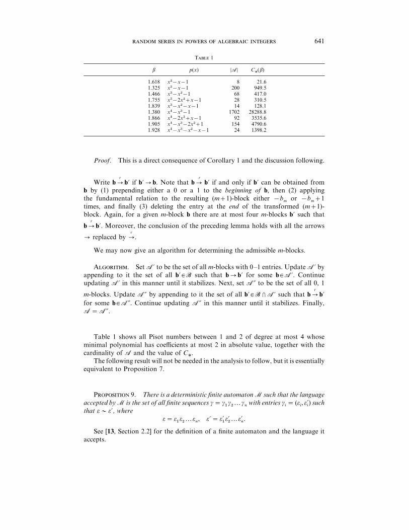
Table 1 shows all Pisot numbers between 1 and 2 of degree at most 4 whose

minimal polynomial has coefficients at most 2 in absolute value, together with the

cardinality of ! and the value of Ck.

The following result will not be needed in the analysis to follow, but it is essentially

equivalent to Proposition 7.

P 9. There is a deterministic finite automaton - such that the language

accepted by - is the set of all finite sequences γ¯ γ"γ#…γ

nwith entries γ

i¯ (ε

i, ε!

i) such

that εC ε«, where

ε¯ ε"ε#…ε

n, ε«¯ ε!

"ε!#…ε!

n.

See [13, Section 2.2] for the definition of a finite automaton and the language it

accepts.

642 .

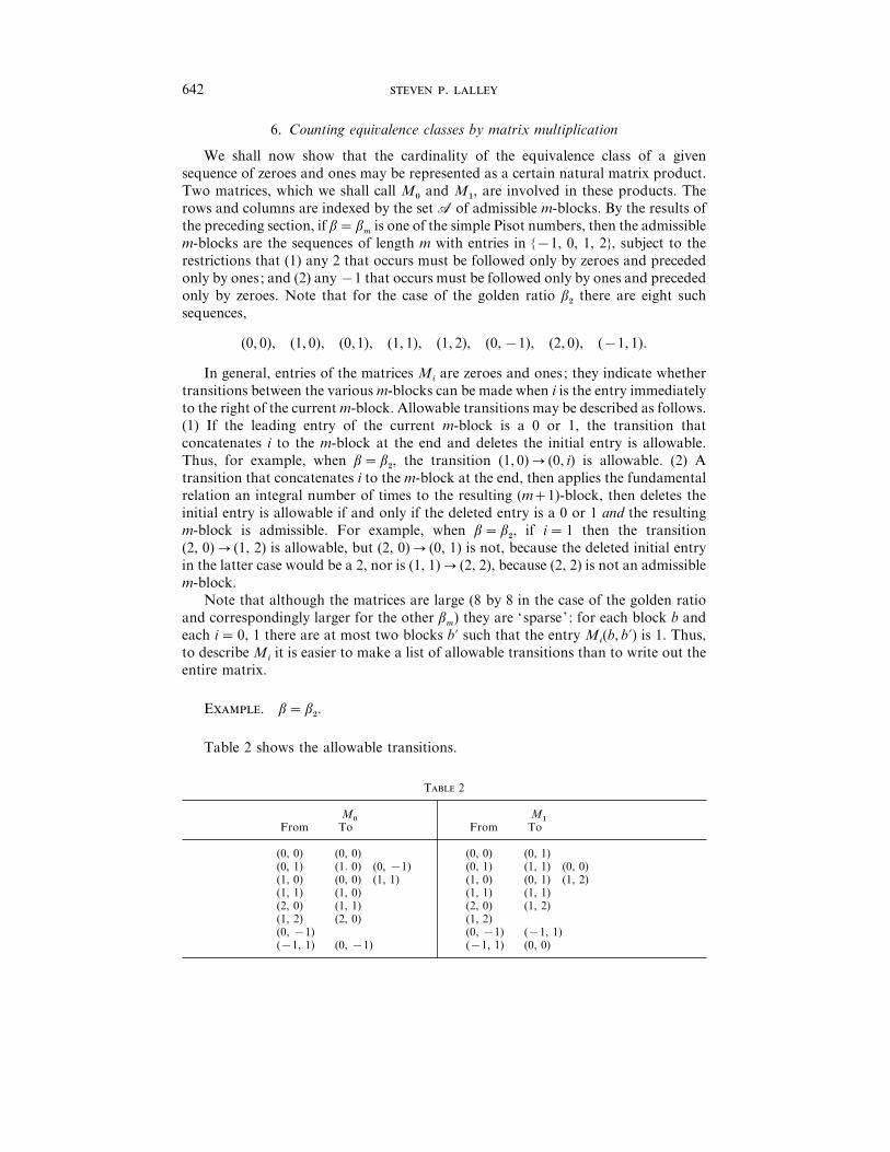
6. Counting equi�alence classes by matrix multiplication

We shall now show that the cardinality of the equivalence class of a given

sequence of zeroes and ones may be represented as a certain natural matrix product.

Two matrices, which we shall call M!

and M", are involved in these products. The

rows and columns are indexed by the set ! of admissible m-blocks. By the results of

the preceding section, if β¯ βm

is one of the simple Pisot numbers, then the admissible

m-blocks are the sequences of length m with entries in ²®1, 0, 1, 2´, subject to the

restrictions that (1) any 2 that occurs must be followed only by zeroes and preceded

only by ones; and (2) any ®1 that occurs must be followed only by ones and preceded

only by zeroes. Note that for the case of the golden ratio β#

there are eight such

sequences,

(0, 0), (1, 0), (0,1), (1, 1), (1, 2), (0,®1), (2, 0), (®1, 1).

In general, entries of the matrices Miare zeroes and ones; they indicate whether

transitions between the various m-blocks can be made when i is the entry immediately

to the right of the current m-block. Allowable transitions may be described as follows.

(1) If the leading entry of the current m-block is a 0 or 1, the transition that

concatenates i to the m-block at the end and deletes the initial entry is allowable.

Thus, for example, when β¯ β#, the transition (1, 0)! (0, i) is allowable. (2) A

transition that concatenates i to the m-block at the end, then applies the fundamental

relation an integral number of times to the resulting (m­1)-block, then deletes the

initial entry is allowable if and only if the deleted entry is a 0 or 1 and the resulting

m-block is admissible. For example, when β¯ β#, if i¯ 1 then the transition

(2, 0)! (1, 2) is allowable, but (2, 0)! (0, 1) is not, because the deleted initial entry

in the latter case would be a 2, nor is (1, 1)! (2, 2), because (2, 2) is not an admissible

m-block.

Note that although the matrices are large (8 by 8 in the case of the golden ratio

and correspondingly larger for the other βm) they are ‘sparse ’ : for each block b and

each i¯ 0, 1 there are at most two blocks b« such that the entry Mi(b, b«) is 1. Thus,

to describe Miit is easier to make a list of allowable transitions than to write out the

entire matrix.

E. β¯ β#.

Table 2 shows the allowable transitions.

T 2

M!

M"

From To From To

(0, 0) (0, 0) (0, 0) (0, 1)(0, 1) (1. 0) (0, ®1) (0, 1) (1, 1) (0, 0)(1, 0) (0, 0) (1, 1) (1, 0) (0, 1) (1, 2)(1, 1) (1, 0) (1, 1) (1, 1)(2, 0) (1, 1) (2, 0) (1, 2)(1, 2) (2, 0) (1, 2)(0, ®1) (0, ®1) (®1, 1)(®1, 1) (0, ®1) (®1, 1) (0, 0)

643

Notice that in M!

there are no allowable transitions from the m-block (0, ®1).

This is because a ®1 must always be followed by a 1 in an m-block. But notice also

that there is an allowable transition from (0, ®1) in the matrix M".

P 10. Let ε¯ ε"ε#…ε

n+mbe an arbitrary sequence of zeroes and ones.

Then the number of sequences of zeroes and ones equi�alent to ε and ending in the m-

block b"¯ ε!

"ε!#…ε!

mis the (b

!, b

")th entry of the matrix product Mε

m+"

Mεm+#

…Mεn+m

,

where b!¯ ε

"ε#…ε

m.

It obviously follows that the total number of 0–1 sequences equivalent to ε

is the sum over all m-blocks b"

of the (b!,b

")th entries of the matrix product

Mεm+"

Mεm+#

…Mεn+m

.

Proof. We prove a slightly more general statement, specifically, that for any

admissible m-blocks b!, b

"the (b

!, b

")th entry of Mε

m+"

Mεm+#

…Mεn+m

is the number of

allowable left-right transformations of the sequence b!εm+"

εm+#

…εn+m

ending in a

sequence whose first n entries are zeroes and ones and whose last m entries are the m-

block b". The proof is by induction on n& 1. The case n¯ 1 is easily checked: the

matrices M!

and M"

were defined in such a way that this would be true.

The induction step is also easy. Assume that it is true for all integers less than n

and let ε¯ ε"ε#…ε

n+mbe a sequence of zeroes and ones. Then we know by the

induction hypothesis that the number of canonical (left-right) transformations of the

sequence b!εm+"

εm+#

…εn+m−"

, that move the ‘cursor’ n®1 steps to the right and result

in a sequence beginning with n®1 zeroes and ones and end in a given block b, is the

(b!, b)th entry of Mε

m+"

…Mεn+m−"

. To obtain the number of canonical transformations

of b!εm+"

εm+#

…εn

that move the cursor n steps to the right and transform the final

m-block to b", partition the count by the possible values of the next-to-last m-block

b (when the cursor is n®1 units to the left). Regardless of the steps taken to reach b

the number of ways to go from b to b"is given by the (b, b

")th entry of Mε

n+m

, again

by the induction hypothesis. (Notice that, once the first n®1 steps of the substitution

sequence have been made, the first n®1 entries of the resulting transformed sequence

play no further role, since the cursor has now moved to their right. Therefore, even

though different substitution sequences may result in transformed sequences with

different initial (n®1)-blocks, as long as they result in the same m-block b to the right

of the cursor the number of ways to complete the transformation will be the same for

each.) Finally, summing over all possible m-blocks b and using the definition of

matrix multiplication one obtains the desired equality, completing the inductive phase

of the proof.

It now follows that the asymptotic behavior of the random variable πn(ε) when

ε", ε

#,… is a sequence of i.i.d. Bernoulli-"

#random variables is determined by that of

the random matrix product

Πn¯Mε

m+"

Mεm+#

…Mεn

.

The asymptotic behavior of these random matrix products is in turn described by the

Furstenberg–Kesten theorem ([10] ; also [4, Chapter 1]). This theorem implies that

limn!¢

1

nlog sΠ

ns¯ λ, (9)

644 .

where

λ¯ limn!¢

1

nE log sΠ

ns

is the ‘ top Lyapunov exponent’ of the sequence Πn. Neither the convergence nor the

value of λ is affected by the choice of norm.

If the entries of Πn

were eventually positive, with probability 1, then not only the

norm but also the individual entries would grow exponentially at the rate λ. This is

not the case, however. For example, examination of the entries of M!, M

"in the case

β¯ β#

(see above) shows that the (1, 1) and (1, 0) columns of Πn

cannot both have

positive entries. But the (Euclidean) norms of the rows do grow exponentially at rate

λ, as the following result shows. For any b `!, let ub be the vector with bth entry 1

and all other entries 0.

P 11. For each b `!, we ha�e

limn!¢

su!bΠ

ns"/n ¯ eλ.

Proof. First, we shall argue that for each pair b, b« of admissible m-blocks there

exists a sequence i"i#…i

kof zeroes and ones such that the (b, b«) entry of M

i"

Mi#

…Mik

is positive. Write b! b« if there is such a sequence. Let b, b« be arbitrary admissible

m-blocks. By the definition of !, for each b `! there exist m-blocks b§, b¨ with

0–1 entries such that b! b§ and b¨! b. Consequently, it suffices to prove the

contention only for pairs of m-blocks b, b« with all entries in ²0, 1´. But if b, b« have

only 0–1 entries, then it is certainly true that b! b«, because all the m-blocks in the

concatenation bb« are 0–1 m-blocks and are therefore admissible ; and hence, if b«¯i"i#…i

m, then the b, b« entry of M

i"

Mi#

…Mim

is positive.

Next, we shall argue that with probability 1 there exists an admissible m-block b

(possibly random) so that

lim infn!¢

su!b Πns"/n & eλ. (10)

Since the entries of Πn

and ub are all nonnegative, and since 3b`! ub is the vector with

all entries 1, it follows that s3b`! u!b Πns& sΠ

ns. Consequently, by the Furstenberg–

Kesten theorem, there exists an admissible m-block b such that

lim supn!¢

su!b Πns"/n & eλ.

But since sΠns"/n ! eλ, an elementary argument shows that lim sup may be replaced

by lim inf in the above equation.

The proposition follows from the results of the last two paragraphs. Choose an

admissible m-block bk such that, with positive probability, (10) holds for b¯ bk. Fix

any b `! ; then by the result of the first paragraph (and the fact that the matrices in

the product Πn

are i.i.d.) there exist (random) N"!N

#!I such that the bkth entry

of u!b ΠNj

is a least 1. Hence, for each j¯ 1, 2,… and each n& 1, we have

su!b ΠNj+ns& su!bk Π−"

Nj

ΠNj+n

s.

645

Now consider the sequence of sequences ²u!bk Π−"Nj

ΠNj+n

´n&

", for j¯ 1, 2,…. By the

Kolmogorov 0–1 Law, this sequence is ergodic, since the invariant σ-algebra is

contained in the tail σ-algebra of the sequence ε", ε

#,…. Moreover, by the choice of

bk, the probability that (10) holds for any one of these sequences is p" 0.

Consequently, by the Birkhoff ergodic theorem, with probability 1 there exists j& 1

such that

lim infn!¢

su!bk Π−"Nj

ΠNj+n

s"/n & eλ.

The proposition now follows directly from this and the last displayed inequality.

Let !!

be the set of all admissible m-blocks with only 0–1 entries, and let �¯3b`!

!

ub. Let 1¯3b`! ub be the vector with all entries 1, and let w¯ 1®�.

C 3. For each b `!!, we ha�e

limn!¢

(u!b Πn�)"/n ¯ eλ.

Proof. Recall that for each b `! there exist a finite 0–1 sequence ib ¯ i"i#…i

J

and an admissible m-block b« with 0–1 entries such that the (b, b«) entry of Mi"

Mi#

IM

iJ

is at least 1. Moreover, there exists K!¢ such that the length J of the string ibsatisfies J%K for all b `!, because there are only finitely many b `!.

Let u be a vector with nonnegative entries, not all 0. For each k& 1 let b(k) `! be

such that the b(k) entry of u«Πk

is maximal. (Note that b(k) is random.) For each

k& 1 it may happen, with probability at least 2−K, that εk+j

¯ ijc1% j% J, where

i"i#…i

Jis a 0–1 sequence as in the previous paragraph, for b¯ b(k). Denote this event

by Gk. Since P(G

k)& 2−K for each k, and since the events G

K, G

#K,… are independent,

the Borel–Cantelli lemma implies that

P((5n−K

k=n−onG

k)c i.o.)¯ 0.

We shall argue that on the event 5n−K

k=n−onG

k,

u«Πn�&

su«Πns

r!r$maxn−on%k%n

sΠ−"k

πns. (11)

This will prove the corollary, because by the preceding proposition su«Πns"/n ! eλ,

and, by Lemma 7 below,

lim supn!¢

maxn−on%k%n

sΠ−"k

Πns"/n % 1.

On the event Gk, there is at least one b« `!

!and 1% J%K such that the b« entry

of u«Πk+J

is at least as large as the b(k) entry of u«Πk. Since b« `!

!, there is at least one

b§ `!!

such that the (b«, b§) entry of Π−"k+J

Πn

is at least 1. Consequently,

u«Πn�& u«Π

k+Jub,& u«Π

kub(k) & su«Π

ks}r!r,

the last inequality because of the choice of b(k). On the other hand, no entry of u«Πn

can be larger than su«Πks sΠ−"

kΠ

ns, and hence

su«Πns% r!r# su«Π

ks sΠ−"

kΠ

ns.

646 .

The inequality (11) follows from the last two displayed inequalities.

L 7. lim supn!¢ max

n−on%k%nsΠ−"

kΠ

ns"/n % 1.

Proof. Recall that the random matrices Mεi

can assume only two values, so

EsMεi

s¯ ρ!¢. Now each Π−"k

Πn

is the product of independent copies of Mε"

, so

for any n®on%k% n and any ε" 0, Markov’s inequality implies that

P²sΠ−"k

Πns" (1­ε)n´% ρon(1­ε)−n.

The probability that sΠ−"k

Πns" (1­ε)n for some n®on%k% n cannot be more

than on times this. Because 3n(on)ρon(1­ε)−n !¢, it follows from the

Borel–Cantelli lemma that, with probability 1, we have

maxn−on%k%n

sΠ−"k

Πns" (1­ε)n

for only finitely many n.

T 3. Let λ be the top Lyapuno� exponent for the sequence Πn

of random

matrix products defined abo�e. If ε¯ ε"ε#…, where ε

",ε

#,… are i.i.d. Bernoulli-"

#then,

with probability 1 we ha�e

limn!¢

πn(ε)"/n ¯ "

#eλ ¯α. (12)

Notice that this proves Theorem 1 in the special case p¯ "

#.

Proof. By Proposition 10, the cardinality of the equivalence class of ε"ε#…ε

nis

u!bΠn�, where b¯ ε

"ε#…ε

m. Consequently, π

n(ε)¯ 2−nu!bΠn

�. By the preceding

corollary, πn(ε)"/n ! eλ}2.

7. Calculating the weight of an equi�alence class

For values of p other than "

#the probabilities π

n(ε) cannot be obtained merely by

enumerating the equivalence classes of the various sequences. Nevertheless, it is still

possible to represent them in terms of a matrix product, with matrices similar,

structurally, to those used to enumerate the classes.

Let ε¯ ε"ε#…ε

nbe a given sequence of zeroes and ones; its probability under the

Bernoulli-p measure is pS(ε)qn−S(ε), where S(ε)¯3n

i="εiis the number of ones in ε.

Observe that not all sequences of length n equivalent to ε have the same

probabilities : for instance,when β¯ β#the sequences 100 and 011 are equivalent, but

the first has probability pq# while the second has probability p#q.

Suppose in general that εCε« ; then by Corollary 1 there is a sequence of left-right

substitutions based on the fundamental relation, some positive and some negative,

transforming ε to ε«. Every time a single positive substitution is made, the likelihood

of the sequence is multiplied by the factor (p}q)κ, where κ is the number of ones on

the left-hand side of the fundamental relation minus the number of ones on the right-

hand side. This is because each time the fundamental relation is applied (in the

positive direction) there is a net increase of κ in the number of ones and a net decrease

of κ in the number of zeroes. Similarly, every time a single negative substitution is

647

made, the likelihood is multiplied by (q}p)κ. Hence the likelihood of ε« is ρ times the

likelihood of ε, where ρ¯ (p}q)Nκ and N is the total number of positive substitutions

minus the total number of negative substitutions in the transformation from ε to ε«.

In the last section we defined matrices Miwith 0–1 entries to indicate whether

transformations between different m-blocks could occur when the entry to the right

of the block was i. We found that the entries of products of these matrices give the

number of ways to do substitutions left to right on the original sequence and arrive at

given m-blocks. If we want to tally total likelihood (relative to the parameter p)

instead of cardinality, then instead of ones as entries we should put a positive number

indicating the (multiplicative) effect on likelihood. Thus, we redefine the matrices M!

and M"as follows. For admissible m-blocks b and b« let the (b, b«)th entry of M

ibe

zero when the transition b! b« is not allowable ; piq"−i when the transition is allowable

and no substitution is made in the transition; and piq"−i¬ν when the transition is

allowable and a substitution is made, where ν¯ (p}q)lκ and l is the number of

substitutions made in the transition (l may be positive or negative). For example,

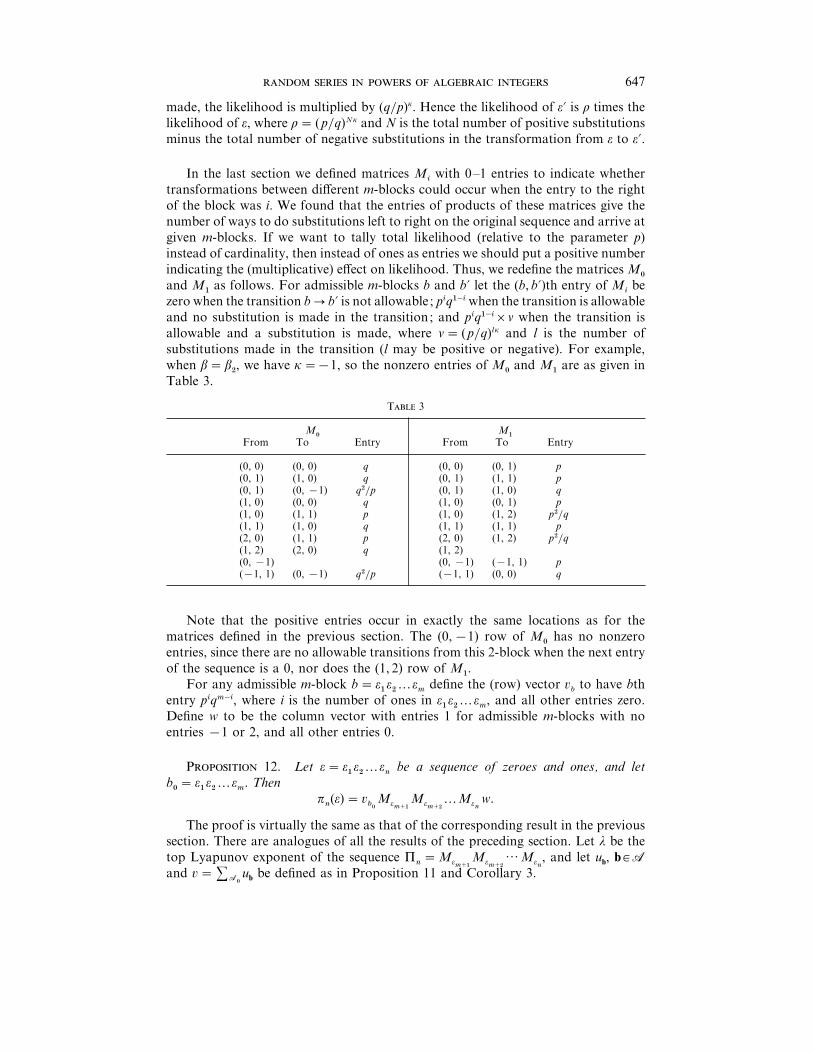
when β¯ β#, we have κ¯®1, so the nonzero entries of M

!and M

"are as given in

Table 3.

T 3

M!

M"

From To Entry From To Entry

(0, 0) (0, 0) q (0, 0) (0, 1) p(0, 1) (1, 0) q (0, 1) (1, 1) p(0, 1) (0, ®1) q#}p (0, 1) (1, 0) q(1, 0) (0, 0) q (1, 0) (0, 1) p(1, 0) (1, 1) p (1, 0) (1, 2) p#}q(1, 1) (1, 0) q (1, 1) (1, 1) p(2, 0) (1, 1) p (2, 0) (1, 2) p#}q(1, 2) (2, 0) q (1, 2)(0, ®1) (0, ®1) (®1, 1) p(®1, 1) (0, ®1) q#}p (®1, 1) (0, 0) q

Note that the positive entries occur in exactly the same locations as for the

matrices defined in the previous section. The (0,®1) row of M!

has no nonzero

entries, since there are no allowable transitions from this 2-block when the next entry

of the sequence is a 0, nor does the (1, 2) row of M".

For any admissible m-block b¯ ε"ε#…ε

mdefine the (row) vector �

bto have bth

entry piqm−i, where i is the number of ones in ε"ε#…ε

m, and all other entries zero.

Define w to be the column vector with entries 1 for admissible m-blocks with no

entries ®1 or 2, and all other entries 0.

P 12. Let ε¯ ε"ε#…ε

nbe a sequence of zeroes and ones, and let

b!¯ ε

"ε#…ε

m. Then

πn(ε)¯ �

b!

Mεm+"

Mεm+#

…Mεn

w.

The proof is virtually the same as that of the corresponding result in the previous

section. There are analogues of all the results of the preceding section. Let λ be the

top Lyapunov exponent of the sequence Πn¯Mε

m+"

Mεm+#

IMεn

, and let ub, b `!and �¯3!

!

ub be defined as in Proposition 11 and Corollary 3.

648 .

P 13. For each b `!!, we ha�e

limn!¢

(u!b Πn�)"/n ¯ eλ.

T 4. Let λ be the top Lyapuno� exponent for the sequence Πn

of random

matrix products defined abo�e. If ε¯ ε"ε#…, where ε

", ε

#…are i.i.d. Bernoulli-p, then

with probability 1 we ha�e

limn!¢

πn(ε)"/n ¯ eλ ¯α. (13)

This completes the proof of Theorem 1.

It should now be clear how to modify the approach for other 0–1 stochastic

sequences, in particular, k-step Markov chains. If k&m then it is necessary to index

the rows and columns by (k­1)-blocks rather than m-blocks, to keep track of the

likelihoods involved. It should also be clear that the whole approach could be adapted

to sequences of random variables valued in other finite subsets of : than ²0, 1´.

8. Computing the Lyapuno� exponent

Computation of Lyapunov exponents is a difficult problem, even for small

matrices. However, because of the special structure of the matrices arising in Sections

6 and 7, computation to a reasonable degree of accuracy is possible for simple Pisot

numbers βm

of small degree m. In this section, we restrict our discussion to the cases

β¯ βm, with m& 2.

Fix a value of the Bernoulli parameter p and let ε", ε

#,…be i.i.d. Bernoulli-p

random variables. Let M!

and M"

be the matrices defined in the preceding section.

Our problem is to calculate the top Lyapunov exponent of the sequence

Πn¯Mε

"

Mε#

…Mεn

.

By Proposition 13, for any vector u with nonnegative entries, not all 0, we have

λ¯ limn!¢

1

nlog suΠ

ns. (14)

A propitious choice is the vector u with (0, 0,…, 0) entry q, (1, 1,…, 1) entry p, and

all other entries 0. (Recall that the rows and columns of the matrices Miare indexed

by admissible m-blocks, hence so are the entries of row vectors.)

The reason for the peculiar choice of u is that the random sequence of vectors uΠn

visits the ray through u infinitely often.

L 8. Let T be the infimum of the set of integers n& 1 such that uΠnis a scalar

multiple of u. Then

ET!¢ ;

in particular, T!¢ with probability 1.

The proof will be given later. In fact, we shall obtain an explicit algebraic (in p)

expression for ET : thus, for instance, when m¯ 2 and p¯ "

#, then ET¯ 12.

649

The existence of such a stopping time allows one to re-express the Lyapunov

exponent in a simpler form. The vector uΠT

is a scalar multiple of the starting vector

u. Since scalars may be factored out of matrix products, this implies that the process

uΠn

effectively ‘regenerates ’ at time T : specifically, the law of the sequence

uΠT+n

suΠTs, n& 0

is the same as that of the original sequence uΠn

with n& 0. It follows that there are

infinitely many times at which uΠn

is a scalar multiple of u ; label these times T!¯

0!T"¯T!T

#!T

$!I!¢. At each of these times the sequence regenerates. For

each n& 1, we have

1

Tn

log suΠTn

s¯1

Tn

3n

j="

logsuΠ

Tj

s

suΠTj−"

s,

and the summands are i.i.d. with finite expectation (this because ET!¢). Dividing

numerator and denominator by n and using the strong law of large numbers on each,

one obtains the limit in (14) along the subsequence Tn

as a ratio of expectations. But

we know the limit in (14) exists, by the Furstenberg–Kesten theorem, so the limit of

the whole sequence must be given by the same ratio of expectations. (Notice that a

standard argument shows that the limit exists without reference to the Furstenberg–

Kesten theorem.) We summarize this in the following corollary.

C 4. We ha�e

λ¯E log suΠ

Ts

ET(15)

and

δ¯E log suΠ

Ts

(log θ)ET. (16)

Since we have an exact expression for ET, only the expectation in the numerator

requires estimation. Unfortunately, no further simplification seems possible : the

numerator can only be estimated by simulation or summation over paths. It should

be remarked, however, that this is a significant improvement on the crude

representation of λ as limn!¢ n−"E log sΠ

ns, because, in general, one cannot say how

fast the convergence in this limit is.

The numerator may, in general, be estimated by simulation with very little effort.

Greater or lesser precision may be obtained by adjusting the number of replications.

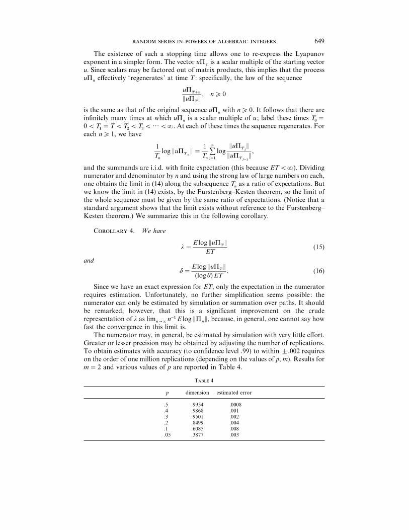
To obtain estimates with accuracy (to confidence level .99) to within ³.002 requires

on the order of one million replications (depending on the values of p, m). Results for

m¯ 2 and various values of p are reported in Table 4.

T 4

p dimension estimated error

.5 .9954 .0008

.4 .9868 .001

.3 .9501 .002

.2 .8499 .004

.1 .6085 .008

.05 .3877 .003

650 .

We have conducted simulations for all rational values of p between 0 and .5 with

denominators less than 12 and also for .01, .02,…, .09; these seem to indicate that the

dimension is a strictly increasing function of p ` (0, .5]. As yet we have no rigorous

argument for this conjecture.

Proof of Lemma 8. We shall discuss only the case m¯ 2, the general case being

completely similar but requiring more cumbersome notation. Thus, u is the vector

with (0, 0) entry q, (1, 1) entry p, and all other entries 0.

Let un¯ uΠ

n. We shall say that any admissible 2-block for which the

corresponding entry of un

is positive occurs in un. Not all admissible 2-blocks may

occur simultaneously in un: for instance, 11 and 10 cannot occur simultaneously.

However, all admissible m-blocks may occur in some un

(see the proof of Proposition

11).

Since the random variables ε", ε

#,… are i.i.d. Bernoulli-p, the sequence must, with

probability 1, contain arbitrarily long blocks of ones. Consider what happens to the

vectors un

when such a long block of ones occurs. If either of the blocks (0, ®1) or

(®1, 1) occurs in un, then after one or two successive ones these blocks will be

converted to the block (0, 0). If either of the blocks (2, 0) or (1, 2) occurs in un, then

after one or two successive ones they will be ‘killed’. If any of the four blocks with

no 2 or ®1 entries occurs in un

then after either one or two successive ones all will

be converted to one of the blocks (0, 0), (0, 1), (1, 1). Consequently, regardless of

which blocks occur in un, if ε

n+"¯ ε

n+#¯ 1 then only 00, 01, and 11 can occur in u

n+#.

Moreover, the blocks 00 and 01 cannot occur simultaneously. Note that if the two

blocks that occur in un+#

are 00 and 11, then if εn+$

¯ 1, the blocks that occur in un+$

must be 01 and 11. Thus, with probability 1, for some n the vector unwill have positive

entries in the 01 and 11 entries and all other entries zero.

Now consider what happens when un

has positive entries in the 01 and 11 entries

and all other entries zero, and εn+"

¯ εn+#

¯ 0. Using Table 2 in Section 6, one easily

verifies that un+#

must have 11 entry pq(un(01)­u

n(11)), 00 entry q#(u

n(01)­u

n(11)),

and all other entries zero. Thus, un+#

is a scalar multiple of u.

The arguments of the last two paragraphs show that, depending on the

composition of un, a regeneration will occur if either (a) ε

n+"¯ 1 and ε

n+#¯ ε

n+$¯ 0,

or (b) εn+"

¯ εn+#

¯ 1 and εn+$

¯ εn+%

¯ 0. Elementary arguments show that this

must happen eventually, with probability 1; in fact, that the expected time until it

happens is finite.

The preceding argument shows that the regeneration event is determined by the

set of admissible m-blocks that occur in a given un

and the subsequent pattern of

zeroes and ones in the sequence εj, but not on the actual coefficients of the m-blocks

that occur in un. It follows that T is a stopping time for the Markov chain whose state

at any time n is the set of admissible m-blocks that occur in un. It follows from

elementary Markov chain theory that ET may be computed by solving a simple

matrix equation. In the special case m¯ 2, there are 7 distinct sets of admissible m-

blocks that may occur simultaneously in un; the transition probabilities between these

sets are easy to write down, and the resulting matrix equation is easily solved via

Mathematica. This yields the identity (when m¯ 2)

ET¯®2®p­p#

®p­2p#®2p$­p%

. (17)

651

Similar formulas may be obtained for arbitrary m, although the size of the matrix

equation that must be solved grows with m.

9. The associated graph

In this section we indicate another approach to the representation of the

probabilities πn(ε) by matrix products. This approach is essentially geometric in

nature, relying on simple properties of a natural graph associated with the Pisot

number β ` (1, 2). In the special case when β is the golden ratio, this graph is the

‘Fibonacci tree ’ exploited by Alexander and Zagier [2].

The (directed) graph Γ¯ (6,% ) is defined as follows. The vertex set 6 is the

union of countably many finite sets 6nwith n& 0; the elements of 6

nare the possible

sums xn(ε)¯3n

k="εkθk, where ε is a 0–1 sequence. The (directed) edges connect

vertices at depths n and n­1: there are edges from xn(ε) to x

n+"(ε) for every ε `Σ, and

no others. To each edge from xn(ε) to x

n(ε)­θn+" attach weight p, and to each edge

from xn(ε) to x

n(ε) attach weight q¯ 1®p.

For any two vertices xn(ε), x

n(ε«) at the same depth n, define their distance

ρ(xn(ε), x

n(ε«)) by

ρ(xn(ε),x

n(ε«))¯ βn rx

n(ε)®x

n(ε«)r.

Fix a constant κ" 2θ}(1®θ). For any vertex xn(ε) define its neighborhood

.(xn(ε))¯.κ(xn

(ε)) to be the set of vertices xn(ε«) at the same depth such that

ρ(xn(ε), x

n(ε«))!κ. Say that two vertices x

n(ε), x

k(ε«) (not necessarily at the same

depth) have the same neighborhood type if there is a bijective mapping between

.(xn(ε)) and .(x

k(ε«)) that preserves the distance function ρ.

P 14. There are only finitely many neighborhood types, that is, there is

a finite set of �ertices 3 such that e�ery �ertex of Γ has the same neighborhood type as

one of the �ertices in 3.

R. The reader should notice the similarity with [5, Theorem], concerning

the Cayley graph of a finitely generated, discontinuous group of isometries of a

hyperbolic space.

Proof. This follows from Garsia’s lemma, which implies that there is a lower

bound d on the ρ-distance between distinct vertices in any neighborhood. Consider

the neighborhoods . of a vertex xn+k

(ε) and . « of the vertex xk(σnε) (here σ is the

shift operator). There is a distance-preserving injection . «!., because there is a

copy Γ« of the graph Γ embedded in Γ emanating from the vertex xn(σnε).

Consequently, for any sequence ε¯ ε"ε#…`Σ and each n& 1 there is a chain of

distance-preserving injections

.(x"(σn−"ε))MN.(x

#(σn−#ε))MN …MN.(x

n(ε)).

By Garsia’s lemma, all sufficiently long chains must stabilize, that is, there is a finite

integer k such that all the injections after the kth in any such chain must be bijections

(if not, there would be neighborhoods with arbitrarily large cardinalities). It follows

that there are only finitely many neighborhood types.

Let 4 be the (finite) set of possible neighborhood types.

652 .

For any vertex xn+"

(ε) at depth n­1& 1, let B(xn+"

(ε))Z6n

be the set of all

vertices at depth n from which emanate directed edges of Γ leading into .(xn+"

(ε)).

L 9. B(xn+"

(ε))Z.(xn(ε)).

Proof. Observe that for any vertex xn+"

(ε«) at depth n­1 there are at most 2, and

at least 1, directed edges from Vn

to xn+"

(ε«). If ε!n+"

¯ 1, then there must be a p-edge

from xn(ε«) to x

n+"(ε«), and there may be a q-edge from some x

n(ε§) to x

n+"(ε«) ; if

ε!n+"

¯ 0, then there must be a q-edge from xn(ε«) to x

n+"(ε«), and there may be a p-edge

from some xn(ε§) to x

n+"(ε«). Consequently, B(x

n+"(ε)) is finite.

Now consider any directed edge from a vertex xn(ε«) `V

nleading into .(x

n+"(ε)).

Depending on whether it is a p-edge or a q-edge,

rxn(ε«)­θn+"®x

n(ε)®ε

n+"θn+"r!κθn+"! 2θn+#}(1®θ)

orrx

n(ε«)®x

n(ε)®ε

n+"θn+"r!κθn+"! 2θn+#}(1®θ).

In either case,

βn rxn(ε«)®x

n(ε)r! θ­2θ#}(1®θ)! 2θ}(1®θ)!κ,

since κ" 2θ}(1®θ).

C 5. For any 0–1 sequence ε¯ ε"ε#… , the neighborhood type

.(xn+"

(ε)) is determined by the neighborhood type .(xn(ε)) and the entry ε

n+".

For any infinite 0–1 sequence ε and each n& 1, define Yn(ε) to be the vector of

probabilitiesYn(ε)¯ (π

n(ε«)).(xn(

ε)),

where the entries are indexed by the elements of .(xn(ε)) (for each element x

n(ε«) of

.(xn(ε)), choose one representative ε« and let π

n(ε«) be the entry for that element). The

probabilities πn(ε) are computed under the Bernoulli-p measure (the measure on

sequence space Σ making ε", ε

#,…, i.i.d. Bernoulli-p random variables).

L 10. There exist nonnegati�e matrices L.,i, for . `4 and i¯ 0, 1, such

that for e�ery 0–1 sequence ε and e�ery n& 1, the identity

Yn+"

(ε)¯L.(xn(ε)),εn+"

Yn(ε) (18)

is satisfied.

Proof. For any sequence ε«¯ ε!"ε!#…the probability π

n+"(ε«) is obtained

by summing the probabilities of all sequences ε§ such that xn+"

(ε§)¯xn+"

(ε«). In

geometric terms, πn+"

(ε) is obtained by summing all πn(ε«)w for depth-n vertices x

n(ε«)

such that there is an edge from xn(ε«) to x

n+"(ε) ; and w¯ p or q, depending on the

weight attached to the edge. Note that there are at most two, and at least one, terms

in this sum. Moreover, by (9), the factors πn(ε«) in the two terms are both entries of

the vector Yn(ε). It is clear that these equations may be written in the matrix form (18),

with the matrix L.(xn(ε)),εn+"

having rows indexed by elements of .(xn+"

(ε)), columns

indexed by elements of .(xn(ε)), and entries 0, p, 1®p.

Note that this argument used the assumption that µ is a Bernoulli measure.

Generalization to arbitrary shift-invariant measures on Σ would seem to be

653

problematic. However, if µ is a Markov measure (that is, under µ the coordinate

process ε", ε

#,… is a k-step Markov chain for some k!¢), then there is an obvious

generalization of Lemma 10. We refrain from giving the details.

Lemma 10 provides a representation of the probability vector Yn(ε) in terms of

matrix products, but, unfortunately, the matrices need not be square. Nevertheless,

it is possible to use the theory of random matrix products to determine the asymptotic

behavior of the sequence Yn(ε). The idea is to embed the vectors Y

n(ε) into vectors

Yn(ε) whose entries are indexed by elements of the union ' of all possible neighborhood

types τ `4, and to embed the matrices L.,i(as blocks) into matrices ,

iwith rows and

columns indexed by elements of '. The entries of Yn(ε) are all zero except for those

indexed by elements of the neighborhood type .(xn(ε) ; these entries have the same

values as the corresponding entries of Yn(ε). Then Lemma 10 implies that Y

n+"(ε)¯

,εn+"

Yn(ε), and consequently, we have the following result.

P 15. If n"k, then

Yn(ε)¯,ε

n

,εn−"

I,εk+"

Yk(ε). (19)

Proposition 15 provides another representation of πn(ε) in terms of a random

matrix product (recall Propositions 10 and 12), as the value of πn(ε) is one of the

entries of the vector Yn(ε). Although this representation is in some ways more natural,

and easier to derive, it seems less useful for actual computations. This is because the

matrices ,i

are, in general, much larger than the matrices in the products in

Propositions 10 and 12, and enumeration of the neighborhood types may be

practically more difficult than the enumeration of the admissible m-blocks for a

given β.

Acknowledgements. Thanks to Irene Hueter for help with some of the numerical

computations and for valuable conversations. Thanks to Yuval Peres for the

reference to [2], and to Boris Solomyak for pointing the author to [9] after seeing an

earlier version of this manuscript.

References

1. J. A and A. Y, ‘Fat baker’s transformations ’, Ergodic Theory Dynamical Systems 4(1984) 1–23.

2. J. A and D. Z, ‘The entropy of a certain infinitely convolved Bernoulli measure’, J.London Math. Soc. (2) 44 (1991) 121–134.

3. T. B, ‘On Weierstrass-like functions and random recurrent sets ’, Math. Proc. CambridgePhilos. Soc. 106 (1989) 325–342.

4. P. B and J. LC, Products of random matrices (Birkhauser, Boston, 1985).5. J. C, ‘The combinatorial structure of co-compact discrete hyperbolic groups’, Geom. Dedicata

16 (1984) 123–148.6. P. E$ , ‘On a family of symmetric Bernoulli convolutions ’, Amer. J. Math. 61 (1939) 974–976.7. P. E$ , ‘On the smoothness of properties of a family of Bernoulli convolutions ’, Amer. J. Math.

62 (1940) 180–186.8. K. F, The geometry of fractal sets (Cambridge University Press, 1985).9. C. F, ‘Representations of numbers and finite automata’. Math. Systems Theory 25 (1992)

37–60.10. H. F and H. K, ‘Products of random matrices ’, Ann. Math. Statistics 31 (1963)

457–469.11. A. G, ‘Arithmetic properties of Bernoulli convolutions ’, Trans. Amer. Math. Soc. 102 (1962)

409–432.12. A. G, ‘Entropy and singularity of infinite convolutions ’, Pacific J. Math. 13 (1963) 1159–1169.13. J. H and J. U, Introduction to automatic theory, languages, and computation (Addison-

Wesley, Reading, 1979).

654

14. R. K and Y. P, ‘ Intersecting random translates of invariant Cantor sets ’, In�ent. Math. 104(1991) 601–629.

15. W. P, ‘On the β expansions of real numbers ’, Acta Math. Acad. Sci. Hun. 11 (1964) 401–416.16. W. P, ‘ Intrinsic Markov chains ’, Trans. Amer. Math. Soc. 112 (1964) 55–64.17. K. P, Ergodic theory (Cambridge University Press, 1983).18. F. P and M. U, ‘On the Hausdorff dimension of some fractal sets ’, Studia Math. 93

(1989) 155–186.19. A. R, ‘Representations for real numbers and their ergodic properties ’, Acta Math. Acad. Sci.

Hung. 8 (1957) 477–493.20. R. S, Algebraic numbers and Fourier analysis (Heath, Lexington, 1963).21. C. L. S, ‘Algebraic integers whose conjugates lie in the unit circle ’, Duke Math. J. 11 (1944)

597–602.22. B. S ‘On the random series Σ³λn, Ann. of Math. (2) 142 (1995) 611–625.23. P. W, An introduction to ergodic theory (Springer, New York, 1982).24. L.-S. Y, ‘Dimension, entropy, and Lyapunov exponents ’, Ergodic Theory Dynamical Systems 2

(1982) 109–124.

Department of StatisticsMathematical Sciences BuildingPurdue UniversityWest LafayetteIndiana 47907USA

E-mail : lalley!stat.purdue.edu