Conjugate Heat Transfer Analysis of Convection-cooled Turbine

Vanes Using γ-Reθ Transition Model

Gang Lin1, Karsten Kusterer1, Anis Haj Ayed1, Dieter Bohn2, Takao Sugimoto3

1 B&B-AGEMA GmbH

Jülicher Strasse 338, 52070 Aachen, Germany

E-mail: lin@bub-agema.de 2RWTH Aachen University

3University of Hyogo

ABSTRACT

In order to achieve high process efficiencies for the economic

operation of stationary gas turbines and aero engines, extremely

high turbine inlet temperatures at adjusted pressure ratios are

applied. The allowable hot gas temperature is limited by the

material temperature of the hot gas path components, in particular

the vanes and blades of the turbine. Thus, intensive cooling is

required to guarantee an acceptable life span of these components.

Modern computational tools as well as advanced calculation

methods support essentially on the successful design of these

thermally high-loaded components. The homogeneous, or

sometimes also mentioned as “full”, conjugate calculation

technique for the coupled calculation of fluid flows, heat transfer

and heat conduction is such an advanced numerical approach in the

design process and huge experiences on validation and application

have been collected throughout the years. This paper summarizes

the numerical approach for this method as well as provides a

collection of numerical results obtained by the authors for

validation cases for a convection-cooled turbine vane test case as

well as comparison to calculation data for this test case provided in

open literature. Furthermore, systematic studies on the impact of

calculation parameters, e.g. hot gas fluid properties, and numerical

models for turbulence calculation are performed and the numerical

results are compared to the experimental results of the test case.

INTRODUCTION

Due to the necessity of cooling technologies in modern gas tur-

bines, turbulent heat transfer is of significant importance in the

thermal design process of the cooled components. Tremendous ef-

forts have been put into the determination of empirical correlations

for the internal and external heat transfer, which are necessary for

the conventional design process. Here, analysis of turbine blade

cooling and heat transfer consists of three areas (Patankar, [1]): (a)

prediction of the heat transfer coefficients on the external surface

of the airfoil (Kays and Crawford, [2]), (b) prediction of heat

transfer in the internal cooling passages (Kays and Crawford, [2])

and (c) calculation of the temperature distribution in the blade ma-

terial.

However, the accuracy of the approach based on heat transfer

coefficients is very much limited by the uncertainties of the

correlations if applied to the real gas turbine geometric

configurations and conditions. With regard to the inter-relations

between the external fluid flow, the internal fluid flow and the heat

conduction, it is obvious that a coupled calculation of the fluid, the

heat transfer and the heat conductivity in the solid body can lead to

a higher accuracy in the design process.

A little bit more than 20 years ago, in the early 1990s, the

Institute of Steam and Gas Turbines at RWTH Aachen University

headed by Prof. Dieter Bohn started a long-term development of a

most sophisticated approach for the coupled calculation of fluid

flows and heat transfer with focus on the hot gas components in a

gas turbine. The numerical group of the institute developed the

homogeneous method for the conjugate calculation technique

(CCT). The method involves the direct coupling of the fluid flow

and the solid body using the same discretization and numerical

principle for both zones. This makes it possible to have an

interpolation-free crossing of the heat fluxes between the

neighboring cell faces. Thus, additional information on the

boundary conditions at the blade walls, such as the distribution of

the heat transfer coefficient, becomes redundant, and the wall

temperatures as well as the temperatures in the blade walls are a

direct result of this simulation. First results and validation cases

have been published in the 1990s for convection-cooled cases (e.g.

[3-6]) as well as for film-cooled configurations (e.g. [7-9]). The

detailed description of the conjugate calculation technique and its

validation is provided by Bohn et al. in [10].

NOMENCLATURE

Flength = function to control transition length

Fonset = function to control transition onset location

H = heat transfer coefficient (W/m2/K)

H0 = reference heat transfer coefficient (1135 W/m2/K )

L = axial chord length (m)

Ma = Mach number

k = turbulent kinetic energy (m2/s2)

Re = momentum thickness Reynolds number

cRe = momentum thickness Reynolds number, where the

intermittency starts to increase

tRe = momentum thickness Reynolds number, where the skin

friction starts to increase

teR~ = transported variable for

tRe

S = streamwise distance

T = temperature (K)

Tref = reference temperature (811K)

X = axiale chord position (m)

y+ = non-dimensional wall-normal distance,

γ = intermittency

μ = dynamic viscosity (kg/m/s)

μt = turbulent viscosity (kg/m/s)

International Journal of Gas Turbine, Propulsion and Power Systems December 2014, Volume 6, Number 3

Copyright © 2014 Gas Turbine Society of Japan

Manuscript Received on November 20, 2013 Review Completed on November 26, 2014

9

ρ = density (kg/m3)

ω = specific turbulence dissipation rate (s-1)

TEST CASE DESCRIPTION

The famous Mark II test case for a convection-cooled vane has

been chosen for comparative calculations of the thermal load by

application of the CCT. The vane has been investigated extensively

by Hylton et al. [11] over a wide range of operating conditions in a

hot gas duct. Mark II is a high-pressure turbine nozzle guide vane,

which is convectively cooled with air by ten radial cooling channels.

Figure 1 shows the vane geometry and the arrangement of the

cooling passages. The test case no. 5411 has been chosen for the

numerical investigations. The numerical validations have been

carried out in both 2-D and 3-D cases. In 2-D case the heat transfer

coefficients and cooling air temperatures have been defined as

boundary conditions for calculation of heat transfer from internal

cooling air. In 3-D case the heat transfer from internal cooling air to

solid is calculated by given cooling air mass flow and cooling air

inlet temperature. After Hylton et al. [11] the inlet turbulence

intensity was 6.5% in the experiment, which has also be used in the

numerical investigations. Instead of turbulence length scale the

turbulent viscosity ratio has been applied as another inlet boundary

condition for turbulence conditions. The inlet turbulent viscosity

ratio has been set at 10. In the study by Mansour et al. [12] the inlet

turbulent viscosity ratio has insignificant impact on the heat

transfer coefficient distribution prediction at suction side in the case

Mark II.

Fig. 1 Geometry and boundary conditions for Mark II test case

The own-developed solver, CHTflow, is based on the

homogeneous method as it is described in [10]. Conjugate

calculations have been performed with structured hexahedral grids

for 2-D case. The y+ in the boundary layer is approximately y+=1.

The Baldwin-Lomax algebraic turbulence model [13] has been

applied. The model has been established during the validation

procedure of the CHTflow code in the mid 1990s and the results

have been presented in [4, 10]. These results are taken as the

reference for the present calculations with commercial CFD

software. In the recent years, this kind of homogeneous conjugate

methodology found its way also into the commercial CFD codes

and, thus, the Star CCM+ solver [14] has been applied for the new

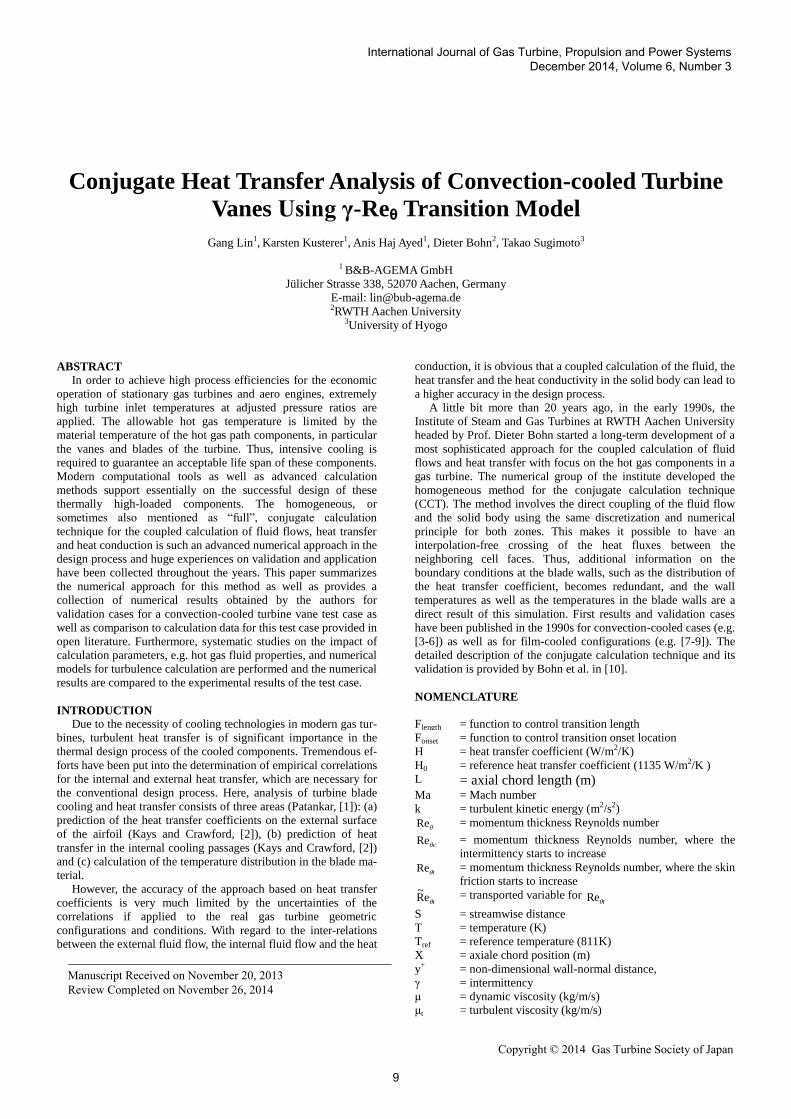
calculation and comparison to the CHTflow results. Figure 2 shows

the mid-section of the 3-D polyhedral mesh, which has been used

for the CCM+ application. In order to establish an appropriate

calculation of the local heat transfer, the y+ value of the first cell in

the boundary layer is less than y+=1. The suitable cell number of the

grid after mesh independency study is 2.86 million including the

prism layers on the fluid-solid boundaries. Best results have been

obtained with the SST k-ω turbulence model and if not otherwise

mentioned, presented results from the CCM+ solver have been

obtained by application of this model.

Fig. 2 Mid-section of 3D polyhedral mesh for CCM+ application

The SST turbulence model [15] is a two-equation turbulence

model, which combines the advantages of both k-ω and k-ε model.

With the help of a blending function F1, the turbulence model can

be transformed between k-ε model in the freestream zone and κ-ω

model in the boundary layer zone. With this method, the advantages

of near-wall performance of k-ω model can be implemented

without any influence on sensitivity of any boundary condition in

free stream, which can lead to errors in the original k-ω model. The

equations of two transport models, one for turbulent kinetic energy

k and the other for specific turbulence dissipation rate ω, are given

as follows:

k

kk

Dt

Dk

eff

j

j

teffj

tk

j xu

Sxx

1,1.0,maxmin

2

xx

F

xu

Sxx

jj

j

j

tj

tj

k

kDt

D

112

21

22

Usually the γ-Reθ transition model is applied in the SST

turbulence model [15]. This transition model is build up by two

transport equations: one is for the intermittency γ and the other is

for the transported transition momentum thickness Reynolds

number teR

~ .

cFc

cFcFxx

eturba

eonsetalength

j

t

j

SDt

D

22

1

5.0

1

1

1

JGPP Vol.6, No. 3

10

F

cxx

tt

tt

j

t

tt

j

t U

Dt

D

1)eR~

(500

eR~

eR~

Re2

The intermittency γ determines the production of turbulent

kinetic energy in the boundary layer. It is 0 in the laminar boundary

layer and 1 in the fully turbulent layer. teR

~ is used as the criterion

of transition onset position, which transforms non-local free stream

information into a local quantity. So that the function Fonset (shown

in eq. 3), which is used to control transition onset location, can be

expressed.

Open literature numerical data by other authors for this test

configuration can be found in [16-19], for example, as well as

numerical data [20-24] for the similar C3X test case from Hylton et

al. [11]. The same test configuration Mark II has been studied by

Yan et al. [16] using a structured mesh in the commercial solvers

CFX and Fluent with different turbulence models. The results of

SST Gamma Theta calculation in CFX solver have shown a good

agreement with the experimental data in temperature distribution.

The temperature at the reattachment point on suction side was over

predicted by about 6% to 7%. Lin et al. [17] have done the analysis

of this test case also in the CFX solver but using unstructured mesh

with the SST-γ-Reθ model. The numerical results capture the trends

of temperature along the surface with an under prediction by about

5% to 8% on the pressure side. Zeng and Qing [18] have completed

another 2D and 3D conjugate heat transfer simulation of Mark II

with unstructured mesh. The grid in the 3D calculation was

obtained by extruding of the 2D grid. The boundary conditions in

the cooling channels, for both 2D and 3D simulation, were applied

with cooling temperature and heat transfer coefficient. The SST-

γ-Reθ model again showed the best accuracy among all of the used

turbulence models. The maximum difference between prediction

and test data occurred at the reattachment point with about 3% to

4% over prediction.

RESULTS

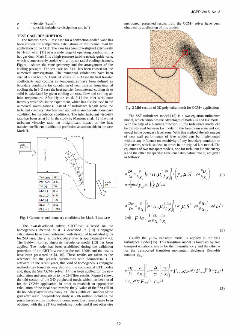
Both applied numerical codes show reasonable results for the

Mach-number distribution in the mid-section of the vane as it is

compared in Fig. 3. There is a strong and sharp compression shock

on the front part of the vane suction side. In front of the shock the

flow is accelerated up a Mach-number of slightly over Ma=1.6.

Downstream the strong shock, the flow is accelerated again, before

a second, weaker shock can be observed shortly in front of the

trailing edge.

a) CHT flow result

b) CCM+ result

Fig. 3 Mach-number distribution (mid-section)

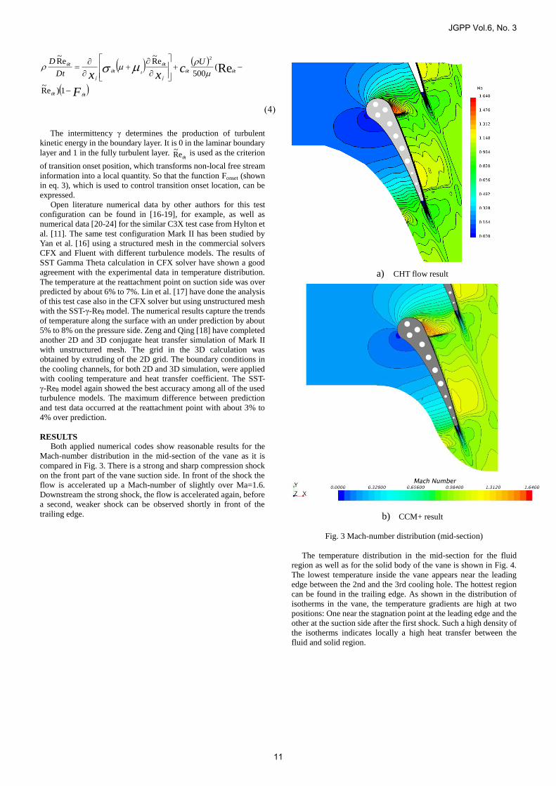
The temperature distribution in the mid-section for the fluid

region as well as for the solid body of the vane is shown in Fig. 4.

The lowest temperature inside the vane appears near the leading

edge between the 2nd and the 3rd cooling hole. The hottest region

can be found in the trailing edge. As shown in the distribution of

isotherms in the vane, the temperature gradients are high at two

positions: One near the stagnation point at the leading edge and the

other at the suction side after the first shock. Such a high density of

the isotherms indicates locally a high heat transfer between the

fluid and solid region.

JGPP Vol.6, No. 3

11

a) CHT flow result

b) CCM+ result

Fig. 4 Temperature distribution (mid-section)

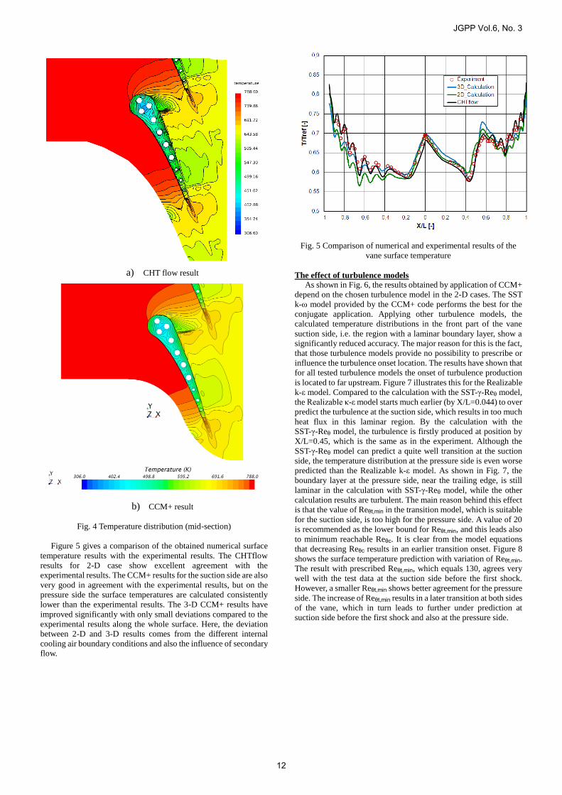
Figure 5 gives a comparison of the obtained numerical surface

temperature results with the experimental results. The CHTflow

results for 2-D case show excellent agreement with the

experimental results. The CCM+ results for the suction side are also

very good in agreement with the experimental results, but on the

pressure side the surface temperatures are calculated consistently

lower than the experimental results. The 3-D CCM+ results have

improved significantly with only small deviations compared to the

experimental results along the whole surface. Here, the deviation

between 2-D and 3-D results comes from the different internal

cooling air boundary conditions and also the influence of secondary

flow.

Fig. 5 Comparison of numerical and experimental results of the

vane surface temperature

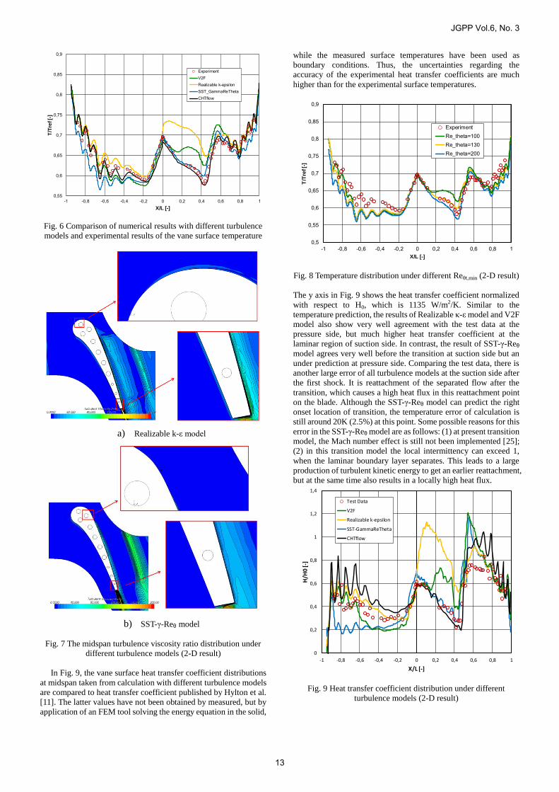
The effect of turbulence models

As shown in Fig. 6, the results obtained by application of CCM+

depend on the chosen turbulence model in the 2-D cases. The SST

k-ω model provided by the CCM+ code performs the best for the

conjugate application. Applying other turbulence models, the

calculated temperature distributions in the front part of the vane

suction side, i.e. the region with a laminar boundary layer, show a

significantly reduced accuracy. The major reason for this is the fact,

that those turbulence models provide no possibility to prescribe or

influence the turbulence onset location. The results have shown that

for all tested turbulence models the onset of turbulence production

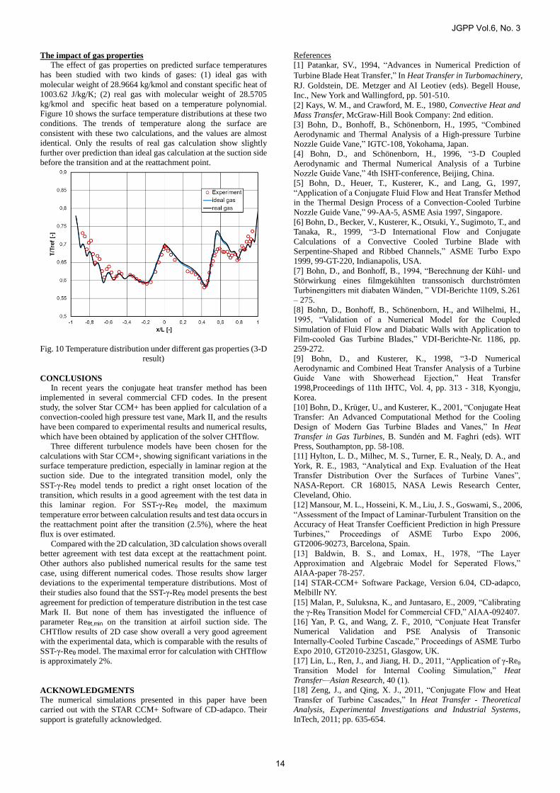
is located to far upstream. Figure 7 illustrates this for the Realizable

k-ε model. Compared to the calculation with the SST-γ-Reθ model,

the Realizable κ-ε model starts much earlier (by X/L=0.044) to over

predict the turbulence at the suction side, which results in too much

heat flux in this laminar region. By the calculation with the

SST-γ-Reθ model, the turbulence is firstly produced at position by

X/L=0.45, which is the same as in the experiment. Although the

SST-γ-Reθ model can predict a quite well transition at the suction

side, the temperature distribution at the pressure side is even worse

predicted than the Realizable k-ε model. As shown in Fig. 7, the

boundary layer at the pressure side, near the trailing edge, is still

laminar in the calculation with SST-γ-Reθ model, while the other

calculation results are turbulent. The main reason behind this effect

is that the value of Reθt,min in the transition model, which is suitable

for the suction side, is too high for the pressure side. A value of 20

is recommended as the lower bound for Reθt,min, and this leads also

to minimum reachable Reθc. It is clear from the model equations

that decreasing Reθc results in an earlier transition onset. Figure 8

shows the surface temperature prediction with variation of Reθt,min.

The result with prescribed Reθt,min, which equals 130, agrees very

well with the test data at the suction side before the first shock.

However, a smaller Reθt,min shows better agreement for the pressure

side. The increase of Reθt,min results in a later transition at both sides

of the vane, which in turn leads to further under prediction at

suction side before the first shock and also at the pressure side.

JGPP Vol.6, No. 3

12

0,55

0,6

0,65

0,7

0,75

0,8

0,85

0,9

-1 -0,8 -0,6 -0,4 -0,2 0 0,2 0,4 0,6 0,8 1

T/T

ref [-

]

X/L [-]

ExperimentV2FRealizable k-epsilonSST_GammaReThetaCHTflow

Fig. 6 Comparison of numerical results with different turbulence

models and experimental results of the vane surface temperature

a) Realizable k-ε model

b) SST-γ-Reθ model

Fig. 7 The midspan turbulence viscosity ratio distribution under

different turbulence models (2-D result)

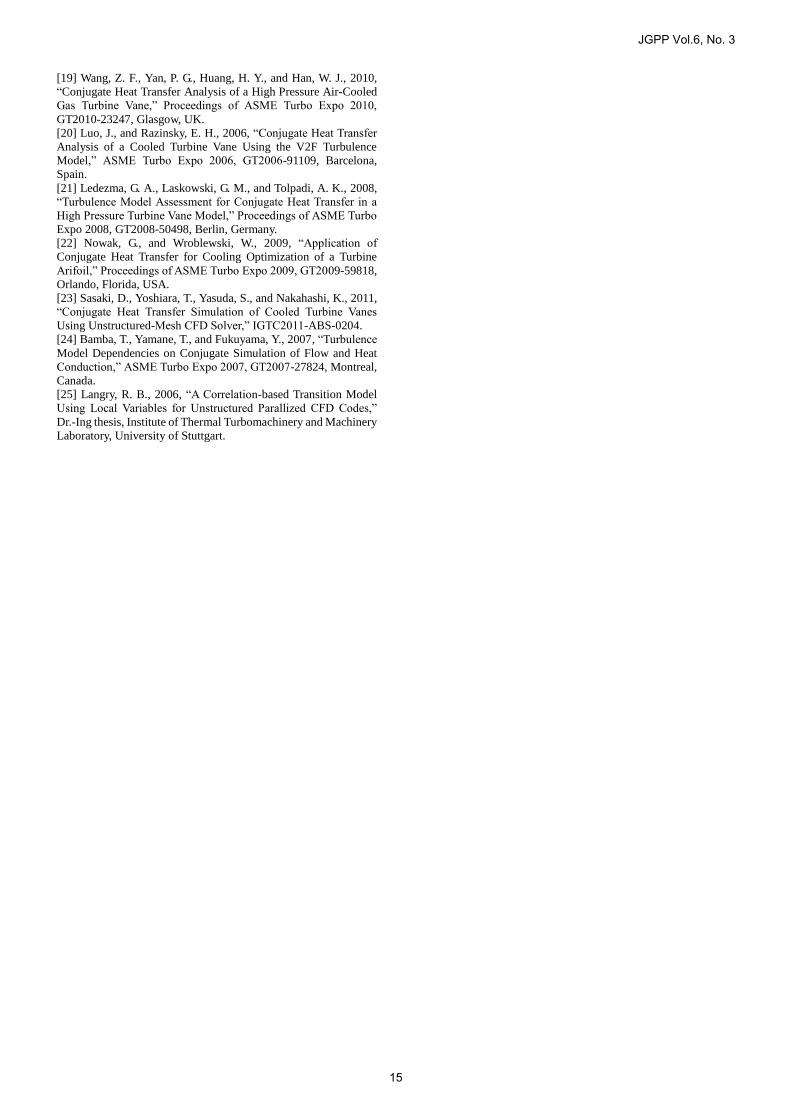
In Fig. 9, the vane surface heat transfer coefficient distributions

at midspan taken from calculation with different turbulence models

are compared to heat transfer coefficient published by Hylton et al.

[11]. The latter values have not been obtained by measured, but by

application of an FEM tool solving the energy equation in the solid,

while the measured surface temperatures have been used as

boundary conditions. Thus, the uncertainties regarding the

accuracy of the experimental heat transfer coefficients are much

higher than for the experimental surface temperatures.

0,5

0,55

0,6

0,65

0,7

0,75

0,8

0,85

0,9

-1 -0,8 -0,6 -0,4 -0,2 0 0,2 0,4 0,6 0,8 1

T/T

ref [-

]

X/L [-]

ExperimentRe_theta=100Re_theta=130Re_theta=200

Fig. 8 Temperature distribution under different Reθt,min (2-D result)

The y axis in Fig. 9 shows the heat transfer coefficient normalized

with respect to H0, which is 1135 W/m2/K. Similar to the

temperature prediction, the results of Realizable κ-ε model and V2F

model also show very well agreement with the test data at the

pressure side, but much higher heat transfer coefficient at the

laminar region of suction side. In contrast, the result of SST-γ-Reθ

model agrees very well before the transition at suction side but an

under prediction at pressure side. Comparing the test data, there is

another large error of all turbulence models at the suction side after

the first shock. It is reattachment of the separated flow after the

transition, which causes a high heat flux in this reattachment point

on the blade. Although the SST-γ-Reθ model can predict the right

onset location of transition, the temperature error of calculation is

still around 20K (2.5%) at this point. Some possible reasons for this

error in the SST-γ-Reθ model are as follows: (1) at present transition

model, the Mach number effect is still not been implemented [25];

(2) in this transition model the local intermittency can exceed 1,

when the laminar boundary layer separates. This leads to a large

production of turbulent kinetic energy to get an earlier reattachment,

but at the same time also results in a locally high heat flux.

0

0,2

0,4

0,6

0,8

1

1,2

1,4

-1 -0,8 -0,6 -0,4 -0,2 0 0,2 0,4 0,6 0,8 1

H/H

0 [-

]

X/L [-]

Test Data

V2F

Realizable k-epsilon

SST-GammaReTheta

CHTflow

Fig. 9 Heat transfer coefficient distribution under different

turbulence models (2-D result)

JGPP Vol.6, No. 3

13

The impact of gas properties

The effect of gas properties on predicted surface temperatures

has been studied with two kinds of gases: (1) ideal gas with

molecular weight of 28.9664 kg/kmol and constant specific heat of

1003.62 J/kg/K; (2) real gas with molecular weight of 28.5705

kg/kmol and specific heat based on a temperature polynomial.

Figure 10 shows the surface temperature distributions at these two

conditions. The trends of temperature along the surface are

consistent with these two calculations, and the values are almost

identical. Only the results of real gas calculation show slightly

further over prediction than ideal gas calculation at the suction side

before the transition and at the reattachment point.

Fig. 10 Temperature distribution under different gas properties (3-D

result)

CONCLUSIONS

In recent years the conjugate heat transfer method has been

implemented in several commercial CFD codes. In the present

study, the solver Star CCM+ has been applied for calculation of a

convection-cooled high pressure test vane, Mark II, and the results

have been compared to experimental results and numerical results,

which have been obtained by application of the solver CHTflow.

Three different turbulence models have been chosen for the

calculations with Star CCM+, showing significant variations in the

surface temperature prediction, especially in laminar region at the

suction side. Due to the integrated transition model, only the

SST-γ-Reθ model tends to predict a right onset location of the

transition, which results in a good agreement with the test data in

this laminar region. For SST-γ-Reθ model, the maximum

temperature error between calculation results and test data occurs in

the reattachment point after the transition (2.5%), where the heat

flux is over estimated.

Compared with the 2D calculation, 3D calculation shows overall

better agreement with test data except at the reattachment point.

Other authors also published numerical results for the same test

case, using different numerical codes. Those results show larger

deviations to the experimental temperature distributions. Most of

their studies also found that the SST-γ-Reθ model presents the best

agreement for prediction of temperature distribution in the test case

Mark II. But none of them has investigated the influence of

parameter Reθt,min on the transition at airfoil suction side. The

CHTflow results of 2D case show overall a very good agreement

with the experimental data, which is comparable with the results of

SST-γ-Reθ model. The maximal error for calculation with CHTflow

is approximately 2%.

ACKNOWLEDGMENTS

The numerical simulations presented in this paper have been

carried out with the STAR CCM+ Software of CD-adapco. Their

support is gratefully acknowledged.

References

[1] Patankar, SV., 1994, “Advances in Numerical Prediction of

Turbine Blade Heat Transfer,” In Heat Transfer in Turbomachinery,

RJ. Goldstein, DE. Metzger and AI Leotiev (eds). Begell House,

Inc., New York and Wallingford, pp. 501-510.

[2] Kays, W. M., and Crawford, M. E., 1980, Convective Heat and

Mass Transfer, McGraw-Hill Book Company: 2nd edition.

[3] Bohn, D., Bonhoff, B., Schönenborn, H., 1995, “Combined

Aerodynamic and Thermal Analysis of a High-pressure Turbine

Nozzle Guide Vane,” IGTC-108, Yokohama, Japan.

[4] Bohn, D., and Schönenborn, H., 1996, “3-D Coupled

Aerodynamic and Thermal Numerical Analysis of a Turbine

Nozzle Guide Vane,” 4th ISHT-conference, Beijing, China.

[5] Bohn, D., Heuer, T., Kusterer, K., and Lang, G., 1997,

“Application of a Conjugate Fluid Flow and Heat Transfer Method

in the Thermal Design Process of a Convection-Cooled Turbine

Nozzle Guide Vane,” 99-AA-5, ASME Asia 1997, Singapore.

[6] Bohn, D., Becker, V., Kusterer, K., Otsuki, Y., Sugimoto, T., and

Tanaka, R., 1999, “3-D International Flow and Conjugate

Calculations of a Convective Cooled Turbine Blade with

Serpentine-Shaped and Ribbed Channels,” ASME Turbo Expo

1999, 99-GT-220, Indianapolis, USA.

[7] Bohn, D., and Bonhoff, B., 1994, “Berechnung der Kühl- und

Störwirkung eines filmgekühlten transsonisch durchströmten

Turbinengitters mit diabaten Wänden, ” VDI-Berichte 1109, S.261

– 275.

[8] Bohn, D., Bonhoff, B., Schönenborn, H., and Wilhelmi, H.,

1995, “Validation of a Numerical Model for the Coupled

Simulation of Fluid Flow and Diabatic Walls with Application to

Film-cooled Gas Turbine Blades,” VDI-Berichte-Nr. 1186, pp.

259-272.

[9] Bohn, D., and Kusterer, K., 1998, “3-D Numerical

Aerodynamic and Combined Heat Transfer Analysis of a Turbine

Guide Vane with Showerhead Ejection,” Heat Transfer

1998,Proceedings of 11th IHTC, Vol. 4, pp. 313 - 318, Kyongju,

Korea.

[10] Bohn, D., Krüger, U., and Kusterer, K., 2001, “Conjugate Heat

Transfer: An Advanced Computational Method for the Cooling

Design of Modern Gas Turbine Blades and Vanes,” In Heat

Transfer in Gas Turbines, B. Sundén and M. Faghri (eds). WIT

Press, Southampton, pp. 58-108.

[11] Hylton, L. D., Milhec, M. S., Turner, E. R., Nealy, D. A., and

York, R. E., 1983, “Analytical and Exp. Evaluation of the Heat

Transfer Distribution Over the Surfaces of Turbine Vanes”,

NASA-Report. CR 168015, NASA Lewis Research Center,

Cleveland, Ohio.

[12] Mansour, M. L., Hosseini, K. M., Liu, J. S., Goswami, S., 2006,

“Assessment of the Impact of Laminar-Turbulent Transition on the

Accuracy of Heat Transfer Coefficient Prediction in high Pressure

Turbines,” Proceedings of ASME Turbo Expo 2006,

GT2006-90273, Barcelona, Spain.

[13] Baldwin, B. S., and Lomax, H., 1978, “The Layer

Approximation and Algebraic Model for Seperated Flows,”

AIAA-paper 78-257.

[14] STAR-CCM+ Software Package, Version 6.04, CD-adapco,

Melbillr NY.

[15] Malan, P., Suluksna, K., and Juntasaro, E., 2009, “Calibrating

the γ-Reθ Transition Model for Commercial CFD,” AIAA-092407.

[16] Yan, P. G., and Wang, Z. F., 2010, “Conjuate Heat Transfer

Numerical Validation and PSE Analysis of Transonic

Internally-Cooled Turbine Cascade,” Proceedings of ASME Turbo

Expo 2010, GT2010-23251, Glasgow, UK.

[17] Lin, L., Ren, J., and Jiang, H. D., 2011, “Application of γ-Reθ

Transition Model for Internal Cooling Simulation,” Heat

Transfer—Asian Research, 40 (1).

[18] Zeng, J., and Qing, X. J., 2011, “Conjugate Flow and Heat

Transfer of Turbine Cascades,” In Heat Transfer - Theoretical

Analysis, Experimental Investigations and Industrial Systems,

InTech, 2011; pp. 635-654.

JGPP Vol.6, No. 3

14

[19] Wang, Z. F., Yan, P. G., Huang, H. Y., and Han, W. J., 2010,

“Conjugate Heat Transfer Analysis of a High Pressure Air-Cooled

Gas Turbine Vane,” Proceedings of ASME Turbo Expo 2010,

GT2010-23247, Glasgow, UK.

[20] Luo, J., and Razinsky, E. H., 2006, “Conjugate Heat Transfer

Analysis of a Cooled Turbine Vane Using the V2F Turbulence

Model,” ASME Turbo Expo 2006, GT2006-91109, Barcelona,

Spain.

[21] Ledezma, G. A., Laskowski, G. M., and Tolpadi, A. K., 2008,

“Turbulence Model Assessment for Conjugate Heat Transfer in a

High Pressure Turbine Vane Model,” Proceedings of ASME Turbo

Expo 2008, GT2008-50498, Berlin, Germany.

[22] Nowak, G., and Wroblewski, W., 2009, “Application of

Conjugate Heat Transfer for Cooling Optimization of a Turbine

Arifoil,” Proceedings of ASME Turbo Expo 2009, GT2009-59818,

Orlando, Florida, USA.

[23] Sasaki, D., Yoshiara, T., Yasuda, S., and Nakahashi, K., 2011,

“Conjugate Heat Transfer Simulation of Cooled Turbine Vanes

Using Unstructured-Mesh CFD Solver,” IGTC2011-ABS-0204.

[24] Bamba, T., Yamane, T., and Fukuyama, Y., 2007, “Turbulence

Model Dependencies on Conjugate Simulation of Flow and Heat

Conduction,” ASME Turbo Expo 2007, GT2007-27824, Montreal,

Canada.

[25] Langry, R. B., 2006, “A Correlation-based Transition Model

Using Local Variables for Unstructured Parallized CFD Codes,”

Dr.-Ing thesis, Institute of Thermal Turbomachinery and Machinery

Laboratory, University of Stuttgart.

JGPP Vol.6, No. 3

15