Computing β-Drawings of 2-Outerplane Graphsmirfan/papers/Irfan_MS_Thesis_2006.pdf · M.Sc. Engg....
80
M.Sc. Engg. Thesis Computing β -Drawings of 2-Outerplane Graphs by Mohammad Tanvir Irfan Submitted to Department of Computer Science and Engineering in partial fulfilment of the requirments for the degree of Master of Science in Computer Science and Engineering Department of Computer Science and Engineering Bangladesh University of Engineering and Technology (BUET) Dhaka 1000 December 2006
-
Upload
truonghanh -
Category
Documents
-
view
221 -
download
2
Transcript of Computing β-Drawings of 2-Outerplane Graphsmirfan/papers/Irfan_MS_Thesis_2006.pdf · M.Sc. Engg....
M.Sc. Engg. Thesis
Computing β-Drawings of 2-Outerplane Graphs
by
Mohammad Tanvir Irfan
Submitted to
Department of Computer Science and Engineering
in partial fulfilment of the requirments for the degree of
Master of Science in Computer Science and Engineering
Department of Computer Science and Engineering
Bangladesh University of Engineering and Technology (BUET)
Dhaka 1000
December 2006
The thesis titled “Computing β-Drawings of 2-Outerplane Graphs,” submittedby Mohammad Tanvir Irfan, Roll No. 040405037P, Session April 2004, to the Department ofComputer Science and Engineering, Bangladesh University of Engineering and Technology, hasbeen accepted as satisfactory in partial fulfillment of the requirements for the degree of Masterof Science in Computer Science and Engineering and approved as to its style and contents.Examination held on December 24, 2006.
Board of Examiners
1.Dr. Md. Saidur Rahman ChairmanProfessor (Supervisor)Department of CSEBUET, Dhaka 1000
2.Dr. Muhammad Masroor Ali MemberProfessor & Head (Ex-officio)Department of CSEBUET, Dhaka 1000
3.Dr. Md. Shamsul Alam MemberProfessorDepartment of CSEBUET, Dhaka 1000
4.Dr. Masud Hasan MemberAssistant ProfessorDepartment of CSEBUET, Dhaka 1000
5.Dr. Md. Abdul Hakim Khan MemberAssociate Professor (External)Department of MathematicsBUET, Dhaka 1000
i

Candidate’s Declaration
It is hereby declared that this thesis or any part of it has not been submitted elsewhere
for the award of any degree or diploma.
Mohammad Tanvir Irfan
Candidate
ii
Contents
Board of Examiners i
Candidate’s Declaration ii
Acknowledgements vii
Abstract viii
1 Introduction 1
1.1 Proximity Graphs . . . . . . . . . . . . . . . . . . . . . . . . . . . . . . . . 1
1.2 Applications of Proximity Graphs . . . . . . . . . . . . . . . . . . . . . . . 2
1.2.1 Dataset Thinning in NN-rule . . . . . . . . . . . . . . . . . . . . . 2
1.2.2 Other Applications . . . . . . . . . . . . . . . . . . . . . . . . . . . 5
1.3 Parameterized Family of Proximity Graphs . . . . . . . . . . . . . . . . . . 6
1.4 Literature Review . . . . . . . . . . . . . . . . . . . . . . . . . . . . . . . . 6
1.4.1 Computation of Proximity Graphs . . . . . . . . . . . . . . . . . . 6
1.4.2 Proximity Graph Drawing . . . . . . . . . . . . . . . . . . . . . . . 8
1.5 Summary . . . . . . . . . . . . . . . . . . . . . . . . . . . . . . . . . . . . 10
1.6 Organization of the Thesis . . . . . . . . . . . . . . . . . . . . . . . . . . . 12
2 Preliminaries 13
2.1 Graphs . . . . . . . . . . . . . . . . . . . . . . . . . . . . . . . . . . . . . . 13
2.2 Planar Graphs and Plane Graphs . . . . . . . . . . . . . . . . . . . . . . . 14
iii
CONTENTS iv
2.3 Straight-line Drawings . . . . . . . . . . . . . . . . . . . . . . . . . . . . . 15
2.4 1-Outerplanar Graphs and 2-Outerplanar Graphs . . . . . . . . . . . . . . 16
2.5 Fan of a Vertex . . . . . . . . . . . . . . . . . . . . . . . . . . . . . . . . . 18
2.6 Complex Cycle . . . . . . . . . . . . . . . . . . . . . . . . . . . . . . . . . 18
2.7 β-Regions . . . . . . . . . . . . . . . . . . . . . . . . . . . . . . . . . . . . 19
2.8 Notions of β-Drawings . . . . . . . . . . . . . . . . . . . . . . . . . . . . . 21
2.8.1 β-drawings . . . . . . . . . . . . . . . . . . . . . . . . . . . . . . . . 21
2.8.2 The β-drawability problem . . . . . . . . . . . . . . . . . . . . . . . 21
2.8.3 Angular measurements related to β-drawings . . . . . . . . . . . . . 22
2.8.4 What values of β are most interesting? . . . . . . . . . . . . . . . . 23
2.8.5 The β-boundary curve . . . . . . . . . . . . . . . . . . . . . . . . . 24
2.9 Chapter Summary . . . . . . . . . . . . . . . . . . . . . . . . . . . . . . . 25
3 β-Drawability of Biconnected 2-Outerplane Graphs 26
3.1 A Necessary Condition for β-Drawability . . . . . . . . . . . . . . . . . . . 26
3.2 Sufficient Conditions . . . . . . . . . . . . . . . . . . . . . . . . . . . . . . 27
3.2.1 Proof of the Sufficient Conditions . . . . . . . . . . . . . . . . . . . 28
3.3 Application . . . . . . . . . . . . . . . . . . . . . . . . . . . . . . . . . . . 55
3.4 Chapter Summary . . . . . . . . . . . . . . . . . . . . . . . . . . . . . . . 58
4 Forbidden 2-Outerplane Graphs 59
4.1 Necessary Condition . . . . . . . . . . . . . . . . . . . . . . . . . . . . . . 60
4.2 Sufficient Condition . . . . . . . . . . . . . . . . . . . . . . . . . . . . . . . 60
4.3 Chapter Summary . . . . . . . . . . . . . . . . . . . . . . . . . . . . . . . 62
5 Conclusion 64
List of Figures
1.1 Training dataset for nearest neighbor decision rule . . . . . . . . . . . . . . 3
1.2 Gabriel graph corresponding to points shown in fig. 1.1 . . . . . . . . . . . 4
1.3 Relative neighborhood graph corresponding to points shown in fig. 1.1 . . . 4
2.1 A graph representing a road network among seven cities. . . . . . . . . . . 13
2.2 A planar graph and a plane graph . . . . . . . . . . . . . . . . . . . . . . . 15
2.3 Two straight-line drawings of the same 1-outerplanar graph . . . . . . . . . 16
2.4 A straight-line drawing of a graph of outerplanarity 2. . . . . . . . . . . . . 16
2.5 Straight-line drawing of a 2-outerplane graph and related notations. . . . . 17
2.6 Fan of a vertex u of a biconnected outerplanar graph and related notions. . 19
2.7 A complex cycle C in a plane graph G. . . . . . . . . . . . . . . . . . . . . 19
2.8 β-region for several values of β. . . . . . . . . . . . . . . . . . . . . . . . . 20
2.9 The angles α(β) and γ(β) for several values of β . . . . . . . . . . . . . . . 23
2.10 Cu,v,β(θ) for −π4≤ θ ≤ π
4and for β = 1.6 and β = 3.0. . . . . . . . . . . . . 24
3.1 Case I in the proof of lemma 3.2.2 . . . . . . . . . . . . . . . . . . . . . . . 28
3.2 Case II in the proof of lemma 3.2.2 . . . . . . . . . . . . . . . . . . . . . . 29
3.3 Base case of drawing a fan Fu, when u has only two neighbors . . . . . . . 33
3.4 Induction step of drawing a fan Fu. . . . . . . . . . . . . . . . . . . . . . . 34
3.5 Justification for selection of regions. . . . . . . . . . . . . . . . . . . . . . . 36
3.6 Regions for positioning Fu and G− V (Fu). . . . . . . . . . . . . . . . . . . 37
v
LIST OF FIGURES vi
3.7 An arc xzy computed in the region R1 . . . . . . . . . . . . . . . . . . . . 38
3.8 Two types of vertices in G− V (Fu): type 1 and type 2 . . . . . . . . . . . 39
3.9 Placement of vertices of type 1B. . . . . . . . . . . . . . . . . . . . . . . . 40
3.10 The internal angle between three type 1 vertices . . . . . . . . . . . . . . . 44
3.11 Placement of the vertices of type 2. . . . . . . . . . . . . . . . . . . . . . . 45
3.12 β-region of v1 and v2 is void of vertices of type 1A and type 1B . . . . . . 47
3.13 β-region of v1 and v2 does not contain any vertex of type 2. . . . . . . . . . 48
3.14 β-region of two adjacent type 2 vertices v1 and v2 is empty. . . . . . . . . . 51
3.15 β-region of a fan vertex and an adjacent type 1 vertex is empty. . . . . . . 53
3.16 β-region of a vertex of Fu and another of type 2 is nonempty. . . . . . . . . 54
3.17 Topology of sensors in a network . . . . . . . . . . . . . . . . . . . . . . . 56
3.18 Placement of sensors . . . . . . . . . . . . . . . . . . . . . . . . . . . . . . 57
4.1 Forbidden class and β-drawable class of biconnected 2-outerplane graphs . 59
4.2 A biconnected 2-outerplane graph not satisfying condition 2(a). . . . . . . 61
4.3 A biconnected 2-outerplane graph not satisfying condition 2(b). . . . . . . 61
4.4 A biconnected 2-outerplane graph not satisfying condition 2(a). . . . . . . 62

Acknowledgments
First of all, I would like to express my profound gratitude to Allah, the almighty and
the merciful, for letting me finish this research work.
I would like to thank my supervisor Professor Dr. Md. Saidur Rahman for introducing
me to the beautiful research world of graph drawing. Geometry has always been the
most appealing field of study to me and I feel myself very much fortunate for studying
computational problems in geometry under the supervision of Professor Dr. Rahman,
who is a preeminent scientist in this field. I thank him for his patience in reviewing my
drafts, for correcting my proofs and language, for suggesting new ways of thinking and
for encouraging me to continue my work.
I would also want to thank the members of the board of examiners for their valuable
suggestions. I thank Professor Dr. Muhammad Masroor Ali, Professor Dr. Md. Shamsul
Alam, Dr. Masud Hasan and Dr. Md. Abdul Hakim Khan.
I am grateful to my family members and friends for their encouragement. I must
acknowledge with thanks the contribution of my father, who is a mathematician, to this
research work. At one moment during the research work I lost my heart. Then I discussed
the seemingly unsolvable problem with my father. Together we discussed the issue and
found out a solution.
Last but not least, I must thank the members of our research group. They gave
me valuable suggestions and listened to all of my presentations. Without their sincere
cooperation and constructive criticism this work would not have been possible.
vii
Abstract
One of the relatively new graph drawing problems is the proximity drawing of graphs.
A proximity drawing of a plane graph G is a straight-line drawing of G with the additional
geometric constraint that two vertices of G are adjacent if and only if the well-defined
“proximity region” of these two vertices does not contain any other vertex. In general,
a proximity drawing of a graph has some appealing features. For example, the group
of vertices which are adjacent to each other tend to stay close together in the proximity
drawing and the vertices that are nonadjacent tend to stay relatively far apart from each
other. These underlying features of a proximity drawing of a graph have made it useful
in many practical application areas. One class of parameterized proximity drawings is
the β-drawing, where the value of the parameter β can be any nonnegative real number
including ∞. The problem of whether a class of graphs is β-drawable, for some value of β,
has been studied for two classes of graphs, namely trees and outerplanar graphs. However,
for larger classes of graphs the problem of β-drawability is still an open problem. In this
thesis we concentrate on the problem of β-drawings of 2-outerplane graphs for 1 < β < 2.
We provide a characterization of a subclass of biconnected 2-outerplane graphs for having
a β-drawing for the specified range of β values. We provide a drawing algorithm as well.
We also identify a subclass of biconnected 2-outerplane graphs that are not β-drawable
for 1 < β < 2.
viii
Chapter 1
Introduction
In general, a graph represents relationships among a set of entities. When each vertex v
of a graph represents a point p in space, the graph takes upon some geometric properties.
There are many graphs that have interesting geometric properties. Such graphs are known
as geometric graphs. Well-known geometric graphs such as Voronoi diagrams, Delaunay
triangulations, convex hulls, visibility graphs, etc. have evolved over time for modeling
and solving various practical problems. Compared to the mentioned geometric graphs,
proximity graphs are relatively new in the field of computational geometry. Still, proximity
graphs have been used in a wide range of applications. In this chapter, first we introduce
proximity graphs. Then we specify several application areas where proximity graphs are
being used. We introduce a parameterized family of proximity graphs, known as the β-
proximity graphs, for 0 ≤ β ≤ ∞. Then we review the literature and finally, state the
results of the thesis.
1.1 Proximity Graphs
Proximity graphs are geometric graphs. Although the notion of “proximity graphs” was
coined in much later, essentially the foundation of this fast expanding field of study has
1
CHAPTER 1. INTRODUCTION 2
been the Gabriel graph, introduced by Gabriel and Sokal in the context of geographic
variation analysis [GS69]. A Gabriel graph is a plane graph in which two vertices are
adjacent if and only if the closed circle having these two vertices as its two antipodal
points contains no other vertex of the graph. Here the closed circle just mentioned is also
known as the proximity region, specifically the Gabriel region, of the two vertices. Like
Gabriel graphs other types of proximity graphs also have a well-defined proximity region.
Proximity regions are also termed as regions of influence by many authors. A definition
of the proximity region is the heart of a proximity graph. In fact, this is the prime reason
why a proximity graph is known as a geometric graph. All the geometric properties of
any proximity graph are just results of the definition of its proximity region. For different
proximity regions we get different proximity graphs although they might have the same
set of points in the plane, each point being represented by a vertex of the corresponding
graph. We clarify this idea in the next section by an example from the application domain
of pattern recognition, more specifically instance-based learning.
1.2 Applications of Proximity Graphs
In this section we specify several applications of proximity graphs with the aim of clarifying
the idea of constructing a proximity graph of a plane graph.
1.2.1 Dataset Thinning in NN-rule
The nearest neighbor classification rule, also known as the NN-rule, is one of the most
famous classification rules in pattern recognition. It has gained its popularity because
of its simplicity and also because of Cover and Hart’s theorem that the probability of a
classification error using the nearest neighbor rule is at most twice the Bayes probability
of classification error [CH67]. It may be mentioned here that the Bayes probability of
classification error is the minimum among all classification rules. The nearest neighbor
CHAPTER 1. INTRODUCTION 3
classification rule says that given a set of N training vectors xi, θiNi=1, where xi =
xi1, xi2, ..., xil is the l-dimensional feature vector of the i-th object and θi is the class of
that object, classify the test feature vector xtest to the class θk if min1≤i≤Nd(xi, xtest) =
d(xk, xtest), where d denotes Euclidean distance. Simply stating, classify a test feature
vector to the class of its nearest training vector. Now what’s the problem of this very
simple approach of classification? The first problem is that for a large value of dataset size
N we need huge storage space. The second and related problem is that of computational
requirement, since we need to find distance of the test feature vector from every training
feature vector to find the minimum distance. For these two reasons researchers have been
looking for ways to reduce the size of the training dataset without incurring too much
degradation in performance. Bhattacharya et. al. has achieved it using two types of
proximity graphs, namely the Gabriel graph and the relative neighborhood graph [BPT92].
They have also provided experimental results showing that training dataset reduction
using Gabriel graph introduces a very low margin of additional error. Next we illustrate
how this reduction in dataset is achieved.
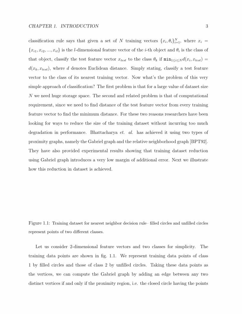
Figure 1.1: Training dataset for nearest neighbor decision rule– filled circles and unfilled circles
represent points of two different classes.
Let us consider 2-dimensional feature vectors and two classes for simplicity. The
training data points are shown in fig. 1.1. We represent training data points of class
1 by filled circles and those of class 2 by unfilled circles. Taking these data points as
the vertices, we can compute the Gabriel graph by adding an edge between any two
distinct vertices if and only if the proximity region, i.e. the closed circle having the points
CHAPTER 1. INTRODUCTION 4
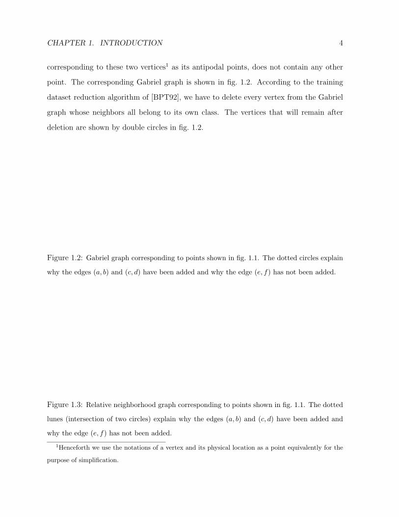
corresponding to these two vertices1 as its antipodal points, does not contain any other
point. The corresponding Gabriel graph is shown in fig. 1.2. According to the training
dataset reduction algorithm of [BPT92], we have to delete every vertex from the Gabriel
graph whose neighbors all belong to its own class. The vertices that will remain after
deletion are shown by double circles in fig. 1.2.
Figure 1.2: Gabriel graph corresponding to points shown in fig. 1.1. The dotted circles explain
why the edges (a, b) and (c, d) have been added and why the edge (e, f) has not been added.
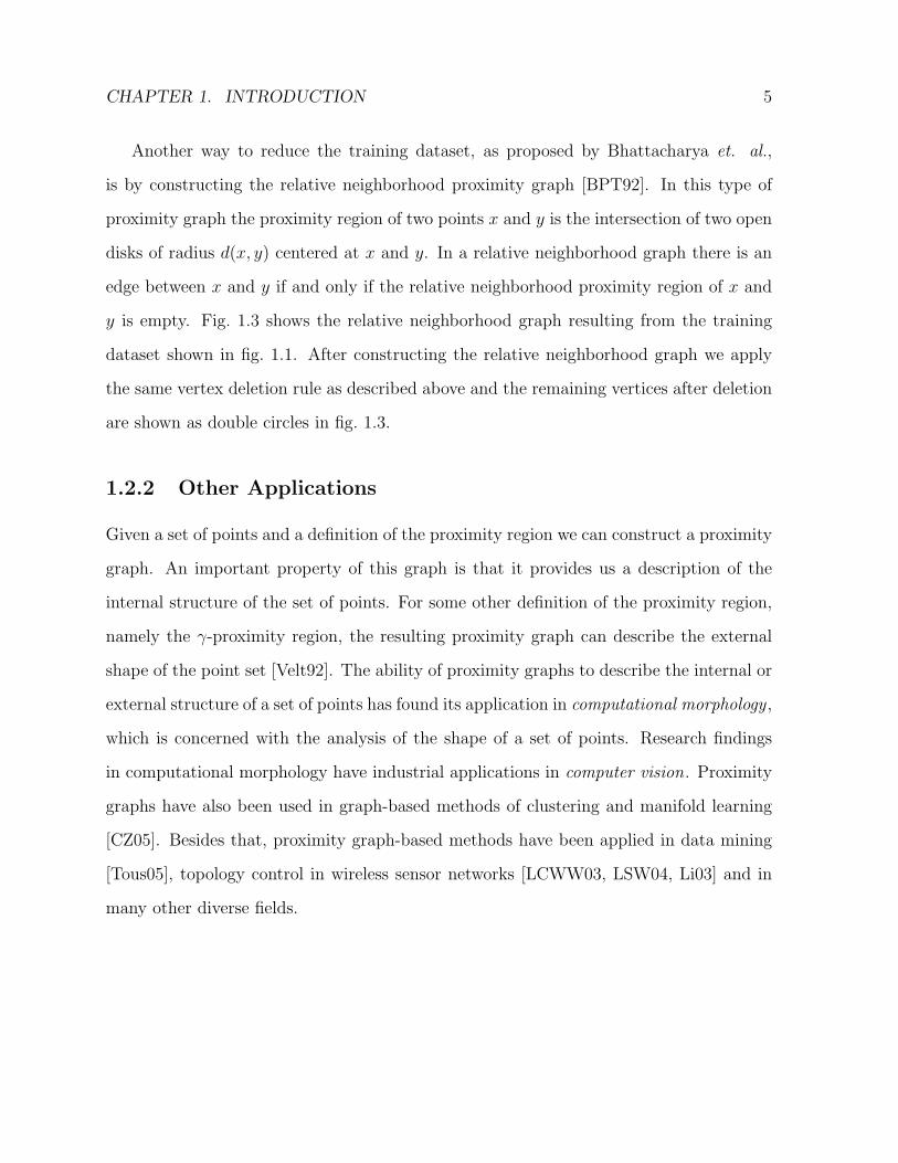
Figure 1.3: Relative neighborhood graph corresponding to points shown in fig. 1.1. The dotted
lunes (intersection of two circles) explain why the edges (a, b) and (c, d) have been added and
why the edge (e, f) has not been added.
1Henceforth we use the notations of a vertex and its physical location as a point equivalently for the
purpose of simplification.
CHAPTER 1. INTRODUCTION 5
Another way to reduce the training dataset, as proposed by Bhattacharya et. al.,
is by constructing the relative neighborhood proximity graph [BPT92]. In this type of
proximity graph the proximity region of two points x and y is the intersection of two open
disks of radius d(x, y) centered at x and y. In a relative neighborhood graph there is an
edge between x and y if and only if the relative neighborhood proximity region of x and
y is empty. Fig. 1.3 shows the relative neighborhood graph resulting from the training
dataset shown in fig. 1.1. After constructing the relative neighborhood graph we apply
the same vertex deletion rule as described above and the remaining vertices after deletion
are shown as double circles in fig. 1.3.
1.2.2 Other Applications
Given a set of points and a definition of the proximity region we can construct a proximity
graph. An important property of this graph is that it provides us a description of the
internal structure of the set of points. For some other definition of the proximity region,
namely the γ-proximity region, the resulting proximity graph can describe the external
shape of the point set [Velt92]. The ability of proximity graphs to describe the internal or
external structure of a set of points has found its application in computational morphology ,
which is concerned with the analysis of the shape of a set of points. Research findings
in computational morphology have industrial applications in computer vision. Proximity
graphs have also been used in graph-based methods of clustering and manifold learning
[CZ05]. Besides that, proximity graph-based methods have been applied in data mining
[Tous05], topology control in wireless sensor networks [LCWW03, LSW04, Li03] and in
many other diverse fields.
CHAPTER 1. INTRODUCTION 6
1.3 Parameterized Family of Proximity Graphs
We have just seen two types of proximity graphs– the Gabriel graph and the relative
neighborhood graph. One might wonder how many other types of proximity graphs are
there. In fact, there is an infinite number of different types of proximity graphs. This is
due to an infinite family of parameterized proximity graphs introduced by Kirkpatrick and
Radke [KR85]. This family of proximity graphs is called β-skeletons, where β stands for
the parameter that can take any real number value in [0,∞]. Interestingly, Gabriel graph
and relative neighborhood graph both belong to this family of proximity graphs. Gabriel
graph is the closed proximity graph for the value of β = 1 and relative neighborhood
graph is the open proximity graph for β = 2.
1.4 Literature Review
Being brought to light in the year of 1969, proximity graphs might seem to be old geometric
graphs. But the most interesting thing is that it has been providing new research trends
quite regularly. In this section we review two basic problems concerning proximity graphs:
firstly, how one can compute a proximity graph when a set of points is given as input and
secondly, how a given plane graph be proximity-drawn.
1.4.1 Computation of Proximity Graphs
The oldest research direction concerning proximity graphs is– given a set of points and
a definition of the proximity region, how can we compute the proximity graph efficiently
and what are the properties of this graph? This research area has been explored and
reviewed very nicely in a paper by Jaromczyk and Toussaint [JT92]. One research prob-
lem in this direction is– what are the lower bounds and upper bounds of the number
of edges in different types of proximity graphs? This would have direct application in
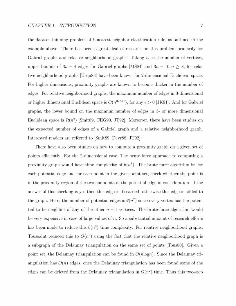
CHAPTER 1. INTRODUCTION 7
the dataset thinning problem of k-nearest neighbor classification rule, as outlined in the
example above. There has been a great deal of research on this problem primarily for
Gabriel graphs and relative neighborhood graphs. Taking n as the number of vertices,
upper bounds of 3n − 8 edges for Gabriel graphs [MS84] and 3n − 10, n ≥ 8, for rela-
tive neighborhood graphs [Urqu83] have been known for 2-dimensional Euclidean space.
For higher dimensions, proximity graphs are known to become thicker in the number of
edges. For relative neighborhood graphs, the maximum number of edges in 3-dimensional
or higher dimensional Euclidean space is O(n3/2+ε), for any ε > 0 [JK91]. And for Gabriel
graphs, the lower bound on the maximum number of edges in 3- or more dimensional
Euclidean space is Ω(n2) [Smit89, CEG90, JT92]. Moreover, there have been studies on
the expected number of edges of a Gabriel graph and a relative neighborhood graph.
Interested readers are referred to [Smit89, Devr88, JT92].
There have also been studies on how to compute a proximity graph on a given set of
points efficiently. For the 2-dimensional case, The brute-force approach to computing a
proximity graph would have time complexity of θ(n3). The brute-force algorithm is: for
each potential edge and for each point in the given point set, check whether the point is
in the proximity region of the two endpoints of the potential edge in consideration. If the
answer of this checking is yes then this edge is discarded, otherwise this edge is added to
the graph. Here, the number of potential edges is θ(n2) since every vertex has the poten-
tial to be neighbor of any of the other n − 1 vertices. The brute-force algorithm would
be very expensive in case of large values of n. So a substantial amount of research efforts
has been made to reduce this θ(n3) time complexity. For relative neighborhood graphs,
Toussaint reduced this to O(n2) using the fact that the relative neighborhood graph is
a subgraph of the Delaunay triangulation on the same set of points [Tous80]. Given a
point set, the Delaunay triangulation can be found in O(nlogn). Since the Delaunay tri-
angulation has O(n) edges, once the Delaunay triangulation has been found some of the
edges can be deleted from the Delaunay triangulation in O(n2) time. Thus this two-step
CHAPTER 1. INTRODUCTION 8
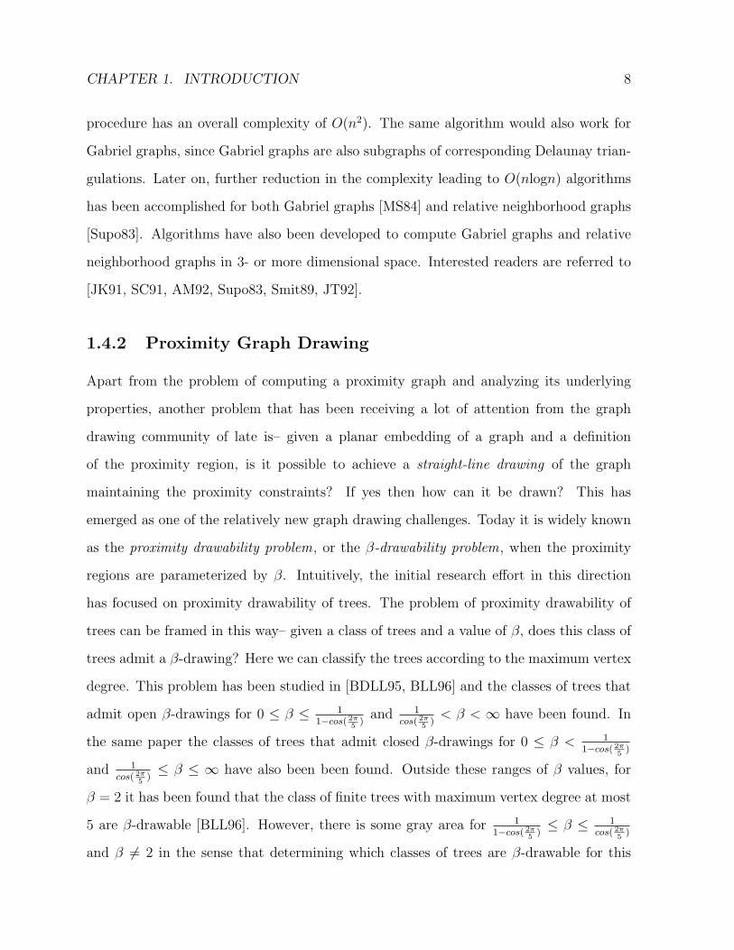
procedure has an overall complexity of O(n2). The same algorithm would also work for
Gabriel graphs, since Gabriel graphs are also subgraphs of corresponding Delaunay trian-
gulations. Later on, further reduction in the complexity leading to O(nlogn) algorithms
has been accomplished for both Gabriel graphs [MS84] and relative neighborhood graphs
[Supo83]. Algorithms have also been developed to compute Gabriel graphs and relative
neighborhood graphs in 3- or more dimensional space. Interested readers are referred to
[JK91, SC91, AM92, Supo83, Smit89, JT92].
1.4.2 Proximity Graph Drawing
Apart from the problem of computing a proximity graph and analyzing its underlying
properties, another problem that has been receiving a lot of attention from the graph
drawing community of late is– given a planar embedding of a graph and a definition
of the proximity region, is it possible to achieve a straight-line drawing of the graph
maintaining the proximity constraints? If yes then how can it be drawn? This has
emerged as one of the relatively new graph drawing challenges. Today it is widely known
as the proximity drawability problem, or the β-drawability problem, when the proximity
regions are parameterized by β. Intuitively, the initial research effort in this direction
has focused on proximity drawability of trees. The problem of proximity drawability of
trees can be framed in this way– given a class of trees and a value of β, does this class of
trees admit a β-drawing? Here we can classify the trees according to the maximum vertex
degree. This problem has been studied in [BDLL95, BLL96] and the classes of trees that
admit open β-drawings for 0 ≤ β ≤ 11−cos( 2π
5)
and 1cos( 2π
5)
< β < ∞ have been found. In
the same paper the classes of trees that admit closed β-drawings for 0 ≤ β < 11−cos( 2π
5)
and 1cos( 2π
5)≤ β ≤ ∞ have also been been found. Outside these ranges of β values, for
β = 2 it has been found that the class of finite trees with maximum vertex degree at most
5 are β-drawable [BLL96]. However, there is some gray area for 11−cos( 2π
5)≤ β ≤ 1
cos( 2π5
)
and β 6= 2 in the sense that determining which classes of trees are β-drawable for this
CHAPTER 1. INTRODUCTION 9
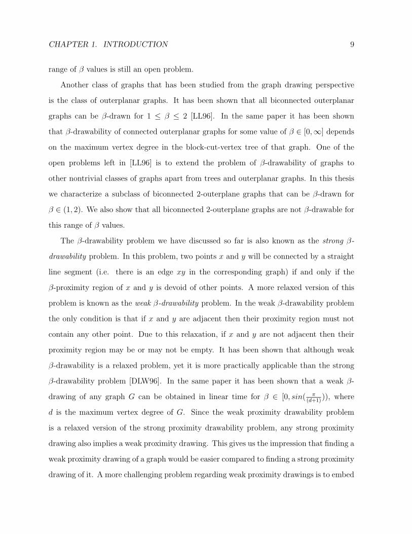
range of β values is still an open problem.
Another class of graphs that has been studied from the graph drawing perspective
is the class of outerplanar graphs. It has been shown that all biconnected outerplanar
graphs can be β-drawn for 1 ≤ β ≤ 2 [LL96]. In the same paper it has been shown
that β-drawability of connected outerplanar graphs for some value of β ∈ [0,∞] depends
on the maximum vertex degree in the block-cut-vertex tree of that graph. One of the
open problems left in [LL96] is to extend the problem of β-drawability of graphs to
other nontrivial classes of graphs apart from trees and outerplanar graphs. In this thesis
we characterize a subclass of biconnected 2-outerplane graphs that can be β-drawn for
β ∈ (1, 2). We also show that all biconnected 2-outerplane graphs are not β-drawable for
this range of β values.
The β-drawability problem we have discussed so far is also known as the strong β-
drawability problem. In this problem, two points x and y will be connected by a straight
line segment (i.e. there is an edge xy in the corresponding graph) if and only if the
β-proximity region of x and y is devoid of other points. A more relaxed version of this
problem is known as the weak β-drawability problem. In the weak β-drawability problem
the only condition is that if x and y are adjacent then their proximity region must not
contain any other point. Due to this relaxation, if x and y are not adjacent then their
proximity region may be or may not be empty. It has been shown that although weak
β-drawability is a relaxed problem, yet it is more practically applicable than the strong
β-drawability problem [DLW96]. In the same paper it has been shown that a weak β-
drawing of any graph G can be obtained in linear time for β ∈ [0, sin( π(d+1)
)), where
d is the maximum vertex degree of G. Since the weak proximity drawability problem
is a relaxed version of the strong proximity drawability problem, any strong proximity
drawing also implies a weak proximity drawing. This gives us the impression that finding a
weak proximity drawing of a graph would be easier compared to finding a strong proximity
drawing of it. A more challenging problem regarding weak proximity drawings is to embed
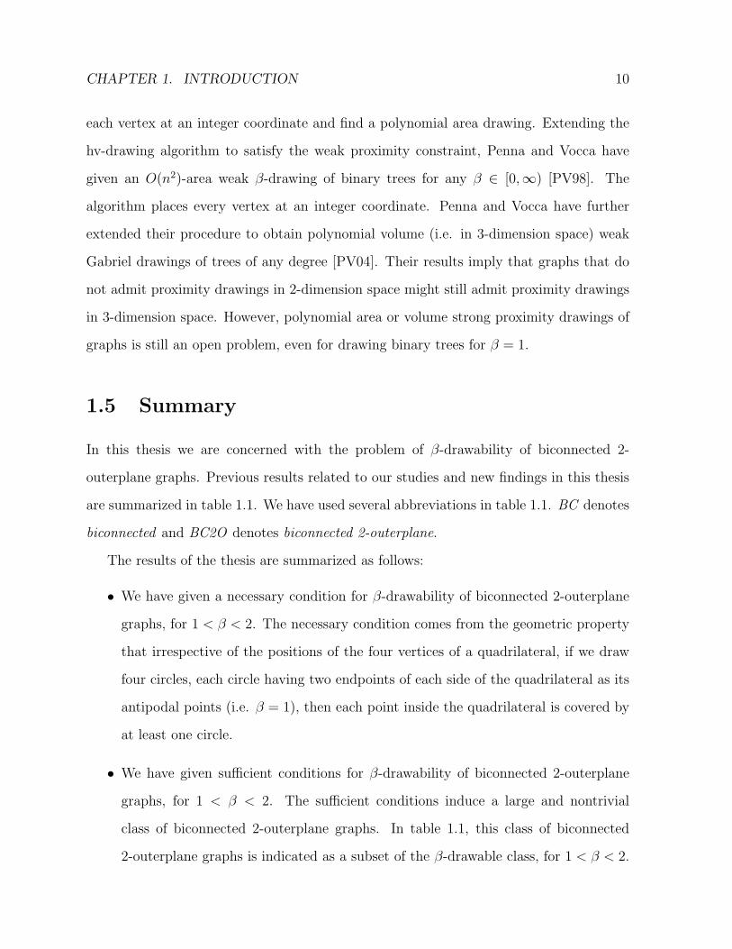
CHAPTER 1. INTRODUCTION 10
each vertex at an integer coordinate and find a polynomial area drawing. Extending the
hv-drawing algorithm to satisfy the weak proximity constraint, Penna and Vocca have
given an O(n2)-area weak β-drawing of binary trees for any β ∈ [0,∞) [PV98]. The
algorithm places every vertex at an integer coordinate. Penna and Vocca have further
extended their procedure to obtain polynomial volume (i.e. in 3-dimension space) weak
Gabriel drawings of trees of any degree [PV04]. Their results imply that graphs that do
not admit proximity drawings in 2-dimension space might still admit proximity drawings
in 3-dimension space. However, polynomial area or volume strong proximity drawings of
graphs is still an open problem, even for drawing binary trees for β = 1.
1.5 Summary
In this thesis we are concerned with the problem of β-drawability of biconnected 2-
outerplane graphs. Previous results related to our studies and new findings in this thesis
are summarized in table 1.1. We have used several abbreviations in table 1.1. BC denotes
biconnected and BC2O denotes biconnected 2-outerplane.
The results of the thesis are summarized as follows:
• We have given a necessary condition for β-drawability of biconnected 2-outerplane
graphs, for 1 < β < 2. The necessary condition comes from the geometric property
that irrespective of the positions of the four vertices of a quadrilateral, if we draw
four circles, each circle having two endpoints of each side of the quadrilateral as its
antipodal points (i.e. β = 1), then each point inside the quadrilateral is covered by
at least one circle.
• We have given sufficient conditions for β-drawability of biconnected 2-outerplane
graphs, for 1 < β < 2. The sufficient conditions induce a large and nontrivial
class of biconnected 2-outerplane graphs. In table 1.1, this class of biconnected
2-outerplane graphs is indicated as a subset of the β-drawable class, for 1 < β < 2.
CHAPTER 1. INTRODUCTION 11
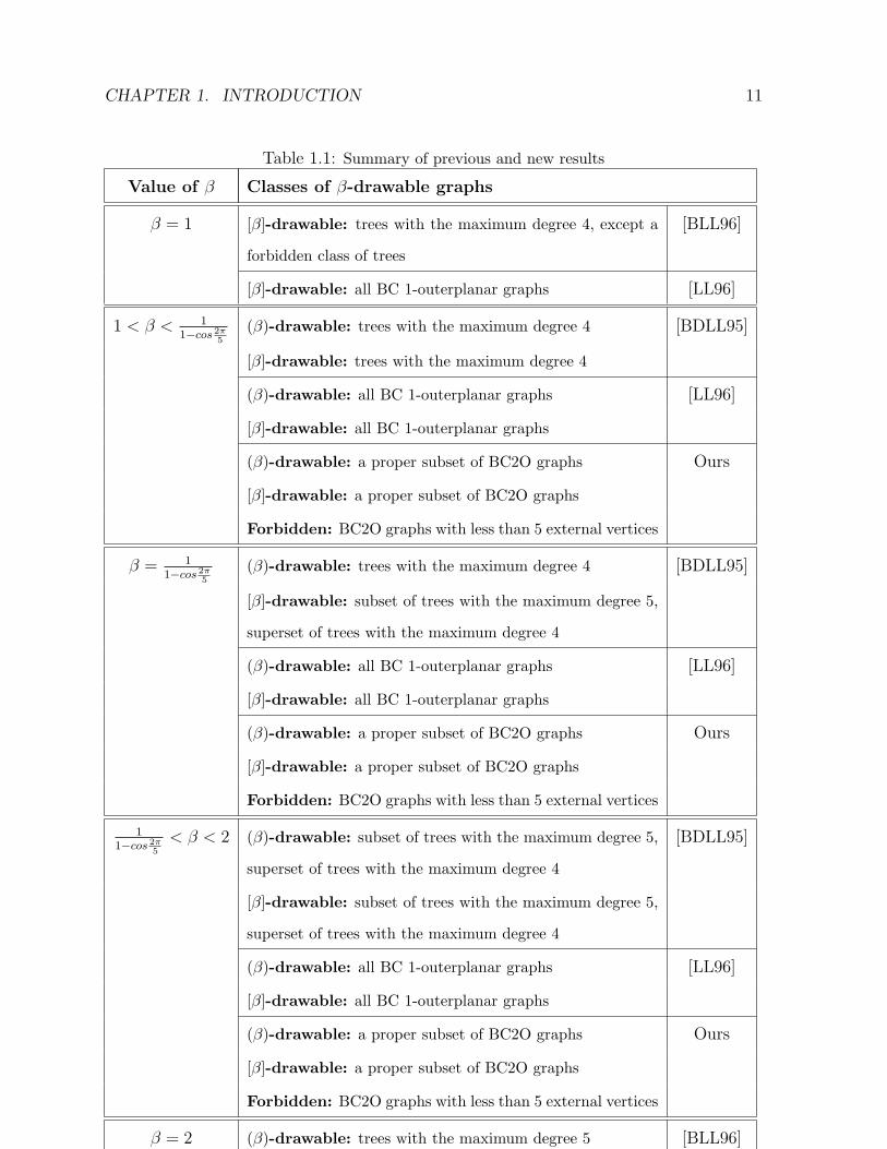
Table 1.1: Summary of previous and new results
Value of β Classes of β-drawable graphs
β = 1 [β]-drawable: trees with the maximum degree 4, except a
forbidden class of trees
[BLL96]
[β]-drawable: all BC 1-outerplanar graphs [LL96]
1 < β < 11−cos 2π
5
(β)-drawable: trees with the maximum degree 4 [BDLL95]
[β]-drawable: trees with the maximum degree 4
(β)-drawable: all BC 1-outerplanar graphs [LL96]
[β]-drawable: all BC 1-outerplanar graphs
(β)-drawable: a proper subset of BC2O graphs Ours
[β]-drawable: a proper subset of BC2O graphs
Forbidden: BC2O graphs with less than 5 external vertices
β = 11−cos 2π
5
(β)-drawable: trees with the maximum degree 4 [BDLL95]
[β]-drawable: subset of trees with the maximum degree 5,
superset of trees with the maximum degree 4
(β)-drawable: all BC 1-outerplanar graphs [LL96]
[β]-drawable: all BC 1-outerplanar graphs
(β)-drawable: a proper subset of BC2O graphs Ours
[β]-drawable: a proper subset of BC2O graphs
Forbidden: BC2O graphs with less than 5 external vertices
11−cos 2π
5
< β < 2 (β)-drawable: subset of trees with the maximum degree 5,
superset of trees with the maximum degree 4
[BDLL95]
[β]-drawable: subset of trees with the maximum degree 5,
superset of trees with the maximum degree 4
(β)-drawable: all BC 1-outerplanar graphs [LL96]
[β]-drawable: all BC 1-outerplanar graphs
(β)-drawable: a proper subset of BC2O graphs Ours
[β]-drawable: a proper subset of BC2O graphs
Forbidden: BC2O graphs with less than 5 external vertices
β = 2 (β)-drawable: trees with the maximum degree 5 [BLL96]
(β)-drawable: all BC 1-outerplanar graphs [LL96]
CHAPTER 1. INTRODUCTION 12
• For a biconnected 2-outerplane graph that satisfies the sufficient conditions, we have
provided an O(n2) drawing algorithm for β-drawing the graph, for 1 < β < 2. This
drawing algorithm is obtained by the constructive proof of the sufficient conditions.
The drawing algorithm requires to find an external vertex that is described as the
“apex”. Finding an apex takes O(n2) time and once an apex is found the remaining
drawing algorithm needs O(n) time.
• The specified necessary condition implies a forbidden class of biconnected 2-outerplane
graphs which cannot be β-drawn, for 1 < β < 2. In table 1.1, this class of bicon-
nected 2-outerplane graphs is indicated as a subset of the forbidden class. The
sufficient conditions imply a subclass of biconnected 2-outerplane graphs that are
β-drawable for the same range of β values. We have shown that if a biconnected
2-outerplane graph does not belong to the forbidden class and also not to the above
mentioned β-drawable class, then this graph is not necessarily β-drawable.
1.6 Organization of the Thesis
The remainder of the thesis is organized as follows. In chapter 2 we state preliminary
definitions, notations and basic properties of proximity drawings. Then in chapter 3
we characterize a subclass of biconnected 2-outerplane graphs that admits β-drawings
for β ∈ (1, 2). In chapter 4, we prove that all biconnected 2-outerplane graphs do not
admit β-drawings for the specified range of β values and we identify a forbidden class of
biconnected 2-outerplane graphs. In chapter 5, we conclude the thesis with an outline of
future research directions related to our studies.
Chapter 2
Preliminaries
In this chapter we first present definitions of graphs, planar and plane graphs, straight-line
drawings of planar graphs, 1-outerplanar and 2-outerplanar graphs and then we define
β-proximity graphs and state several properties of β-drawings of graphs.
2.1 Graphs
A graph is used to model relationships among a set of objects or entities. Mathematically,
a graph G is a tuple (V, E), where V denotes the set of vertices and E denotes the set
of edges, each edge being an unordered pair of vertices. The set of vertices of G is also
denoted by V (G) and the set of edges by E(G).
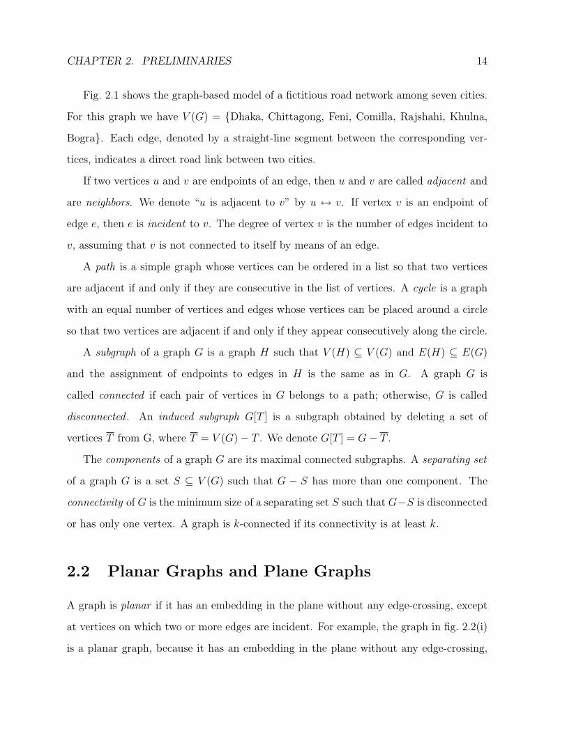
Figure 2.1: A graph representing a road network among seven cities.
13
CHAPTER 2. PRELIMINARIES 14
Fig. 2.1 shows the graph-based model of a fictitious road network among seven cities.
For this graph we have V (G) = Dhaka, Chittagong, Feni, Comilla, Rajshahi, Khulna,
Bogra. Each edge, denoted by a straight-line segment between the corresponding ver-
tices, indicates a direct road link between two cities.
If two vertices u and v are endpoints of an edge, then u and v are called adjacent and
are neighbors. We denote “u is adjacent to v” by u ↔ v. If vertex v is an endpoint of
edge e, then e is incident to v. The degree of vertex v is the number of edges incident to
v, assuming that v is not connected to itself by means of an edge.
A path is a simple graph whose vertices can be ordered in a list so that two vertices
are adjacent if and only if they are consecutive in the list of vertices. A cycle is a graph
with an equal number of vertices and edges whose vertices can be placed around a circle
so that two vertices are adjacent if and only if they appear consecutively along the circle.
A subgraph of a graph G is a graph H such that V (H) ⊆ V (G) and E(H) ⊆ E(G)
and the assignment of endpoints to edges in H is the same as in G. A graph G is
called connected if each pair of vertices in G belongs to a path; otherwise, G is called
disconnected . An induced subgraph G[T ] is a subgraph obtained by deleting a set of
vertices T from G, where T = V (G)− T . We denote G[T ] = G− T .
The components of a graph G are its maximal connected subgraphs. A separating set
of a graph G is a set S ⊆ V (G) such that G − S has more than one component. The
connectivity of G is the minimum size of a separating set S such that G−S is disconnected
or has only one vertex. A graph is k-connected if its connectivity is at least k.
2.2 Planar Graphs and Plane Graphs
A graph is planar if it has an embedding in the plane without any edge-crossing, except
at vertices on which two or more edges are incident. For example, the graph in fig. 2.2(i)
is a planar graph, because it has an embedding in the plane without any edge-crossing,
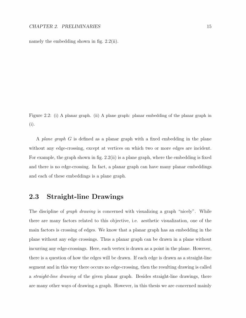
CHAPTER 2. PRELIMINARIES 15
namely the embedding shown in fig. 2.2(ii).
Figure 2.2: (i) A planar graph. (ii) A plane graph: planar embedding of the planar graph in
(i).
A plane graph G is defined as a planar graph with a fixed embedding in the plane
without any edge-crossing, except at vertices on which two or more edges are incident.
For example, the graph shown in fig. 2.2(ii) is a plane graph, where the embedding is fixed
and there is no edge-crossing. In fact, a planar graph can have many planar embeddings
and each of these embeddings is a plane graph.
2.3 Straight-line Drawings
The discipline of graph drawing is concerned with visualizing a graph “nicely”. While
there are many factors related to this objective, i.e. aesthetic visualization, one of the
main factors is crossing of edges. We know that a planar graph has an embedding in the
plane without any edge crossings. Thus a planar graph can be drawn in a plane without
incurring any edge-crossings. Here, each vertex is drawn as a point in the plane. However,
there is a question of how the edges will be drawn. If each edge is drawn as a straight-line
segment and in this way there occurs no edge-crossing, then the resulting drawing is called
a straight-line drawing of the given planar graph. Besides straight-line drawings, there
are many other ways of drawing a graph. However, in this thesis we are concerned mainly
CHAPTER 2. PRELIMINARIES 16
with straight-line drawings.
2.4 1-Outerplanar Graphs and 2-Outerplanar Graphs
An outerplanar graph is a graph that has a planar embedding such that all the vertices
lie on the external face. This graph is also known as a 1-outerplanar graph.
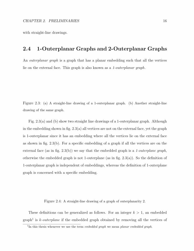
Figure 2.3: (a) A straight-line drawing of a 1-outerplanar graph. (b) Another straight-line
drawing of the same graph.
Fig. 2.3(a) and (b) show two straight line drawings of a 1-outerplanar graph. Although
in the embedding shown in fig. 2.3(a) all vertices are not on the external face, yet the graph
is 1-outerplanar since it has an embedding where all the vertices lie on the external face
as shown in fig. 2.3(b). For a specific embedding of a graph if all the vertices are on the
external face (as in fig. 2.3(b)) we say that the embedded graph is a 1-outerplane graph,
otherwise the embedded graph is not 1-outerplane (as in fig. 2.3(a)). So the definition of
1-outerplanar graph is independent of embeddings, whereas the definition of 1-outerplane
graph is concerned with a specific embedding.
Figure 2.4: A straight-line drawing of a graph of outerplanarity 2.
These definitions can be generalized as follows. For an integer k > 1, an embedded
graph1 is k-outerplane if the embedded graph obtained by removing all the vertices of
1In this thesis whenever we use the term embedded graph we mean planar embedded graph.
CHAPTER 2. PRELIMINARIES 17
the external face is a (k − 1)-outerplane graph. On the other hand, we call a graph
k-outerplanar if it has an embedding that is k-outerplane. A related notion is the out-
erplanarity of a graph which is defined as follows. For an integer k > 0, a graph has
outerplanarity k if k is the least positive integer such that the graph is k-outerplanar.
For example, the graph corresponding to fig. 2.3 is 1-outerplanar as it has a 1-
outerplane embedding (fig. 2.3(b)) and the same graph is also 2-outerplanar as it has
a 2-outerplane embedding (fig. 2.3(a)). Therefore, k = 1 is the least positive integer
such that it is k-outerplanar and thus the outerplanarity of the graph is 1. Fig. 2.4
shows a straight-line drawing of a graph that has no 1-outerplane embedding, but has a
2-outerplane embedding. So the outerplanarity of this graph is 2.
We now define a few notations related to a biconnected 2-outerplane graph.
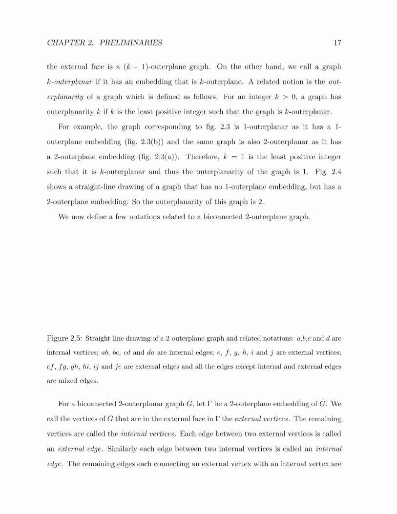
Figure 2.5: Straight-line drawing of a 2-outerplane graph and related notations: a,b,c and d are
internal vertices; ab, bc, cd and da are internal edges; e, f , g, h, i and j are external vertices;
ef , fg, gh, hi, ij and je are external edges and all the edges except internal and external edges
are mixed edges.
For a biconnected 2-outerplanar graph G, let Γ be a 2-outerplane embedding of G. We
call the vertices of G that are in the external face in Γ the external vertices . The remaining
vertices are called the internal vertices . Each edge between two external vertices is called
an external edge. Similarly each edge between two internal vertices is called an internal
edge. The remaining edges each connecting an external vertex with an internal vertex are
CHAPTER 2. PRELIMINARIES 18
called mixed edges . These definitions are illustrated in fig. 2.5.
2.5 Fan of a Vertex
In this section we define the notion of fan of a vertex of a biconnected outerplanar
graph.Let G = (V, E) be a biconnected outerplanar graph. For any vertex u ∈ V , the
fan of u, denoted by Fu, is the subgraph of G induced by the vertices in V that share
an internal face with u in a 1-outerplanar embedding of G. Here, the vertex u is called
the apex of Fu. Since G is outerplanar, Fu is also outerplanar. Let Γ be a 1-outerplanar
embedding of G in which Fu has the 1-outerplanar embedding Φ. Let u1, u2, . . . , uk be
the vertices of neighbors of u in clockwise order in Φ. The edge (u, u1) is called the first
edge of Fu and (u, uk) the last edge of Fu for that embedding. We call each edge (u, ui)
a radial edge of Fu, for i = 2, . . . , k − 1. Apart from the first edge, the last edge and
the radial edges, all other edges of Fu are called fan edges . We denote the m vertices on
the boundary of Φ in between ui and ui+1 by ui,1, ui,2, . . . , ui,m in clockwise order, where
1 ≤ i ≤ k − 1. These notations are illustrated in fig. 2.6.
In this thesis, we adopt the notion of fan of a vertex in a biconnected 2-outerplane
graph by allowing the apex of the fan to be an external vertex of the graph.
2.6 Complex Cycle
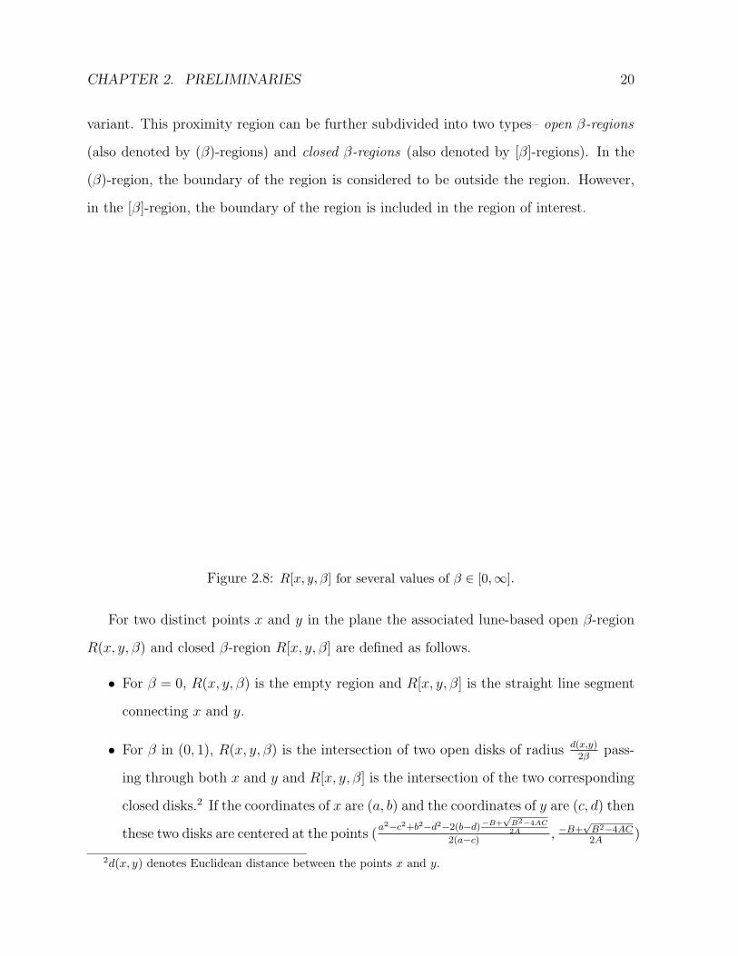
Let C be a cycle in a plane graph G. C is called a complex cycle if there is a vertex
v ∈ V (G) located inside C. If there are k vertices on the complex cycle C then C is called
a complex k-cycle.
Fig. 2.7 shows a complex 4-cycle C in a plane graph G.
CHAPTER 2. PRELIMINARIES 19
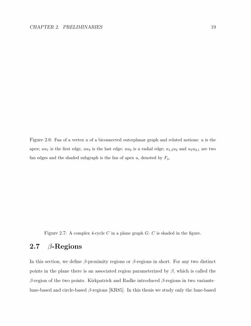
Figure 2.6: Fan of a vertex u of a biconnected outerplanar graph and related notions: u is the
apex; uu1 is the first edge, uu3 is the last edge; uu2 is a radial edge; u1,2u2 and u2u2,1 are two
fan edges and the shaded subgraph is the fan of apex u, denoted by Fu.
Figure 2.7: A complex 4-cycle C in a plane graph G: C is shaded in the figure.
2.7 β-Regions
In this section, we define β-proximity regions or β-regions in short. For any two distinct
points in the plane there is an associated region parameterized by β, which is called the
β-region of the two points. Kirkpatrick and Radke introduced β-regions in two variants–
lune-based and circle-based β-regions [KR85]. In this thesis we study only the lune-based
CHAPTER 2. PRELIMINARIES 20
variant. This proximity region can be further subdivided into two types– open β-regions
(also denoted by (β)-regions) and closed β-regions (also denoted by [β]-regions). In the
(β)-region, the boundary of the region is considered to be outside the region. However,
in the [β]-region, the boundary of the region is included in the region of interest.
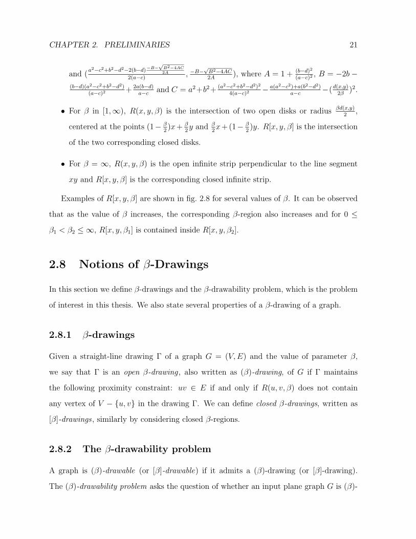
Figure 2.8: R[x, y, β] for several values of β ∈ [0,∞].
For two distinct points x and y in the plane the associated lune-based open β-region
R(x, y, β) and closed β-region R[x, y, β] are defined as follows.
• For β = 0, R(x, y, β) is the empty region and R[x, y, β] is the straight line segment
connecting x and y.
• For β in (0, 1), R(x, y, β) is the intersection of two open disks of radius d(x,y)2β
pass-
ing through both x and y and R[x, y, β] is the intersection of the two corresponding
closed disks.2 If the coordinates of x are (a, b) and the coordinates of y are (c, d) then
these two disks are centered at the points (a2−c2+b2−d2−2(b−d)−B+
√B2−4AC2A
2(a−c), −B+
√B2−4AC2A
)
2d(x, y) denotes Euclidean distance between the points x and y.
CHAPTER 2. PRELIMINARIES 21
and (a2−c2+b2−d2−2(b−d)−B−
√B2−4AC2A
2(a−c), −B−
√B2−4AC2A
), where A = 1 + (b−d)2
(a−c)2, B = −2b−
(b−d)(a2−c2+b2−d2)(a−c)2
+ 2a(b−d)a−c
and C = a2+b2+ (a2−c2+b2−d2)2
4(a−c)2− a(a2−c2)+a(b2−d2)
a−c−(d(x,y)
2β)2.
• For β in [1,∞), R(x, y, β) is the intersection of two open disks or radius βd(x,y)2
,
centered at the points (1− β2)x+ β
2y and β
2x+(1− β
2)y. R[x, y, β] is the intersection
of the two corresponding closed disks.
• For β = ∞, R(x, y, β) is the open infinite strip perpendicular to the line segment
xy and R[x, y, β] is the corresponding closed infinite strip.
Examples of R[x, y, β] are shown in fig. 2.8 for several values of β. It can be observed
that as the value of β increases, the corresponding β-region also increases and for 0 ≤
β1 < β2 ≤ ∞, R[x, y, β1] is contained inside R[x, y, β2].
2.8 Notions of β-Drawings
In this section we define β-drawings and the β-drawability problem, which is the problem
of interest in this thesis. We also state several properties of a β-drawing of a graph.
2.8.1 β-drawings
Given a straight-line drawing Γ of a graph G = (V, E) and the value of parameter β,
we say that Γ is an open β-drawing , also written as (β)-drawing, of G if Γ maintains
the following proximity constraint: uv ∈ E if and only if R(u, v, β) does not contain
any vertex of V − u, v in the drawing Γ. We can define closed β-drawings, written as
[β]-drawings , similarly by considering closed β-regions.
2.8.2 The β-drawability problem
A graph is (β)-drawable (or [β]-drawable) if it admits a (β)-drawing (or [β]-drawing).
The (β)-drawability problem asks the question of whether an input plane graph G is (β)-
CHAPTER 2. PRELIMINARIES 22
drawable or not for a specified value of β. Similarly, the [β]-drawability problem can be
defined.
A class of graphs G is called (β)-drawable if every graph G ∈ G admits a (β)-drawing
[BDLL95]. If there is a graph G ∈ G that does not admit a (β)-drawing then we say that
G is not (β)-drawable. We use similar definition for closed β-drawable class of graphs.
In this thesis we simply use the notations β-regions, β-drawings or β-drawable graphs
whenever the discussion applies for both (β)-regions and [β]-regions.
2.8.3 Angular measurements related to β-drawings
The definitions of β-regions and β-drawings imply that β-drawings are essentially scaling-
independent. That is, if we scale a β-drawing maintaining the aspect ratio, that is the
ration of width and height, then the resulting drawing still maintains the β-proximity
constraints. As a result, lengths of edges or distances among vertices are seldom used
in the analysis of β-drawings of graphs. What actually matters is some form of angular
measurement. In this thesis we use two angular measurements α(β) and γ(β) that are
defined as follows:
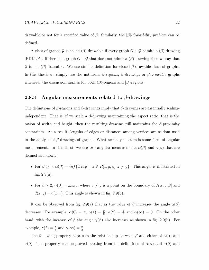
• For β ≥ 0, α(β) = inf∠xzy ‖ z ∈ R[x, y, β], z 6= y. This angle is illustrated in
fig. 2.9(a).
• For β ≥ 2, γ(β) = ∠zxy, where z 6= y is a point on the boundary of R[x, y, β] and
d(x, y) = d(x, z). This angle is shown in fig. 2.9(b).
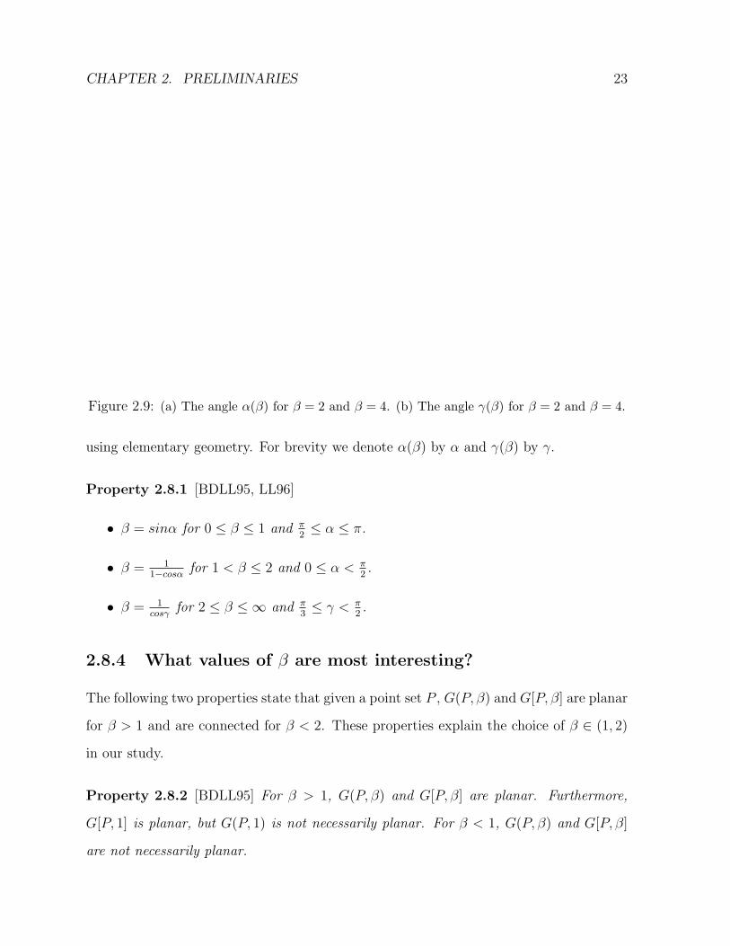
It can be observed from fig. 2.9(a) that as the value of β increases the angle α(β)
decreases. For example, α(0) = π, α(1) = π2, α(2) = π
3and α(∞) = 0. On the other
hand, with the increase of β the angle γ(β) also increases as shown in fig. 2.9(b). For
example, γ(2) = π3
and γ(∞) = π2.
The following property expresses the relationship between β and either of α(β) and
γ(β). The property can be proved starting from the definitions of α(β) and γ(β) and
CHAPTER 2. PRELIMINARIES 23
Figure 2.9: (a) The angle α(β) for β = 2 and β = 4. (b) The angle γ(β) for β = 2 and β = 4.
using elementary geometry. For brevity we denote α(β) by α and γ(β) by γ.
Property 2.8.1 [BDLL95, LL96]
• β = sinα for 0 ≤ β ≤ 1 and π2≤ α ≤ π.
• β = 11−cosα
for 1 < β ≤ 2 and 0 ≤ α < π2.
• β = 1cosγ
for 2 ≤ β ≤ ∞ and π3≤ γ < π
2.
2.8.4 What values of β are most interesting?
The following two properties state that given a point set P , G(P, β) and G[P, β] are planar
for β > 1 and are connected for β < 2. These properties explain the choice of β ∈ (1, 2)
in our study.
Property 2.8.2 [BDLL95] For β > 1, G(P, β) and G[P, β] are planar. Furthermore,
G[P, 1] is planar, but G(P, 1) is not necessarily planar. For β < 1, G(P, β) and G[P, β]
are not necessarily planar.
CHAPTER 2. PRELIMINARIES 24
Property 2.8.3 [BDLL95] For β < 2, G(P, β) and G[P, β] are connected. Furthermore,
G(P, 2) is connected, but G[P, 1] is not necessarily connected. For β > 2, G(P, β) and
G[P, β] are not necessarily connected.
2.8.5 The β-boundary curve
We now define the β-boundary curve that has been introduced by Lenhart and Liotta
[LL96]. For β ∈ [1, 2], any distinct pair of points u and v in the plane is associated with
a β-boundary curve denoted by Cu,v,β such that for every point z on the curve Cu,v,β, v is
on the boundary of R[u, z, β]. Each point z on the curve Cu,v,β is parameterized by the
angle θ ≡ ∠vuz and positive values of θ correspond to the occurrence of u, v and z in
clockwise order.
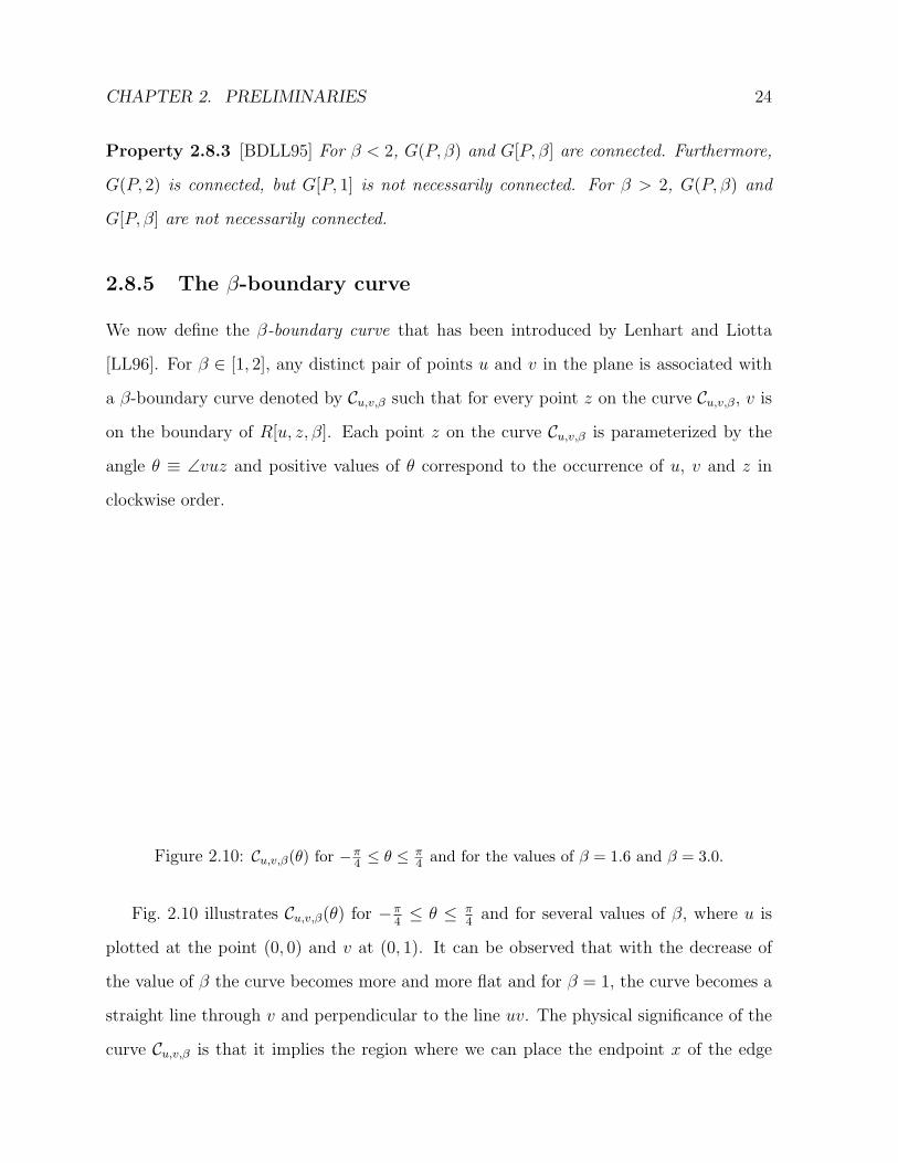
Figure 2.10: Cu,v,β(θ) for −π4 ≤ θ ≤ π
4 and for the values of β = 1.6 and β = 3.0.
Fig. 2.10 illustrates Cu,v,β(θ) for −π4≤ θ ≤ π
4and for several values of β, where u is
plotted at the point (0, 0) and v at (0, 1). It can be observed that with the decrease of
the value of β the curve becomes more and more flat and for β = 1, the curve becomes a
straight line through v and perpendicular to the line uv. The physical significance of the
curve Cu,v,β is that it implies the region where we can place the endpoint x of the edge
CHAPTER 2. PRELIMINARIES 25
(u, x) so that the point v does not lie in the β-region of u and x. For example, if we place
x outside the curve Cu,v,β (w.r.t. u) then v will be inside R[u, x, β]. To the contrary, if we
place x inside Cu,v,β then R[u, x, β] will not contain v.
The following lemma presents the mathematical definition of the β-boundary curve.
Lemma 2.8.1 [LL96] For θ ∈ [−π4, π
4], if u = (0, 0) and v = (0, 1) then
Cu,v,β(θ) =2(√
1−(2/β−1)2sin2θ−(2/β−1)cosθ)
β(1−(2/β−1)2)(sinθ, cosθ).
2.9 Chapter Summary
In this chapter we have defined various notations and terminologies that are used in this
thesis. We have defined graphs, planar and plane graphs, 1-outerplanar and 2-outerplanar
graphs and various other notions. We have also defined the β-drawability problem, on
which we focus in this thesis. We have illustrated the concepts of β-regions and described
several properties of proximity graphs parameterized by β. In the next chapter we are
going to shed light on one of the main works of this thesis– β-drawings of biconnected
2-outerplane graphs. We are going to give a necessary condition and a set of sufficient
conditions for β-drawability of a biconnected 2-outerplane graph.
Chapter 3
β-Drawability of Biconnected
2-Outerplane Graphs
In this chapter we give characterization of biconnected 2-outerplane graphs that can be
β-drawn. We provide a constructive proof of our claim. The constructive prove gives us
an O(n2) drawing algorithm for β-drawing a biconnected 2-outerplane graph that satisfies
a set of sufficient conditions.
3.1 A Necessary Condition for β-Drawability
There are biconnected 2-outerplane graphs that are not β-drawable for β ∈ (1, 2). For
example the graph shown in fig. 2.4 is not β-drawable. In this biconnected 2-outerplane
graph there are four external vertices and one internal vertex. Suppose that we want to
achieve a [1]-drawing of this graph. No matter where we place the four external vertices,
the internal vertex will be inside the proximity region of at least one of the four pairs of
neighboring external vertices. As a result the graph is not [1]-drawable. The graph will
not be β-drawable for β > 1 as well, since the proximity regions will only increase and
we will have no place to position the internal vertex. The same situation will arise for a
26
CHAPTER 3. β-DRAWABILITY OF BICONNECTED 2-OUTERPLANE GRAPHS27
2-outerplane graph with three external vertices. Thus the following lemma holds.
Lemma 3.1.1 Let G be a planar embedded graph. If G has a complex 4-cycle or a complex
3-cycle then G cannot be β-drawn for 1 < β < 2.
From lemma 3.1.1, we can arrive at the following corollary expressing a necessary
condition for β-drawability of a biconnected 2-outerplane graph, for 1 < β < 2.
Corollary 3.1.2 Let G be a biconnected 2-outerplane graph. G has no β-drawing, for
1 < β < 2, if G has less than five external vertices.
3.2 Sufficient Conditions
By definition, corollary 3.1.2 implies that not all of the graphs in the class of biconnected
2-outerplane graphs are β-drawable, for β ∈ (1, 2). We are now interested in finding a
subclass of biconnected 2-outerplane graphs that are β-drawable for 1 < β < 2. The
following theorem characterizes a subclass of biconnected 2-outerplane graphs that are
β-drawable for 1 < β < 2.
Theorem 3.2.1 A biconnected 2-outerplane graph G is β-drawable for β ∈ (1, 2) if G
satisfies the following conditions:
1. There are at least five external vertices; and
2. There is an external vertex u such that the fan Fu has all of the following properties:
(a) Fu is biconnected 1-outerplane;
(b) Fu contains all the internal vertices; and
(c) Every vertex in Fu has at most one neighbor outside Fu and every vertex outside
Fu has at most one neighbor in Fu.
CHAPTER 3. β-DRAWABILITY OF BICONNECTED 2-OUTERPLANE GRAPHS28
3.2.1 Proof of the Sufficient Conditions
In the rest of this chapter we provide a constructive proof of theorem 3.2.1. But before
going on to the proof, an interesting question arises regarding a biconnected 2-outerplane
graph G that satisfies all the conditions in theorem 3.2.1: is there any possibility of the
occurence of a complex 3-cycle or a complex 4-cycle in G? The following lemma confirms
that this can never happen.
Lemma 3.2.2 Let G be a biconnected 2-outerplane graph satisfying the conditions in
theorem 3.2.1. Then a 3-cycle or a 4-cycle of G is a face of G.
Proof. We prove the statement by contradiction. Since G satisfies the conditions
in theorem 3.2.1, G has an external vertex u such that Fu is biconnected 1-outerplane,
contains all the internal vertices and has the property that every vertex in Fu has at most
one neighbor in G− Fu and every vertex in G− Fu has at most one neighbor in Fu.
Suppose that there is a 4-cycle C in G with a vertex v inside the cycle. The following
cases can occur regarding C:
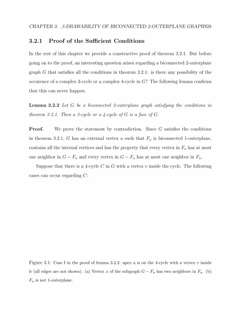
Figure 3.1: Case I in the proof of lemma 3.2.2: apex u is on the 4-cycle with a vertex v inside
it (all edges are not shown). (a) Vertex x of the subgraph G− Fu has two neighbors in Fu. (b)
Fu is not 1-outerplane.
CHAPTER 3. β-DRAWABILITY OF BICONNECTED 2-OUTERPLANE GRAPHS29
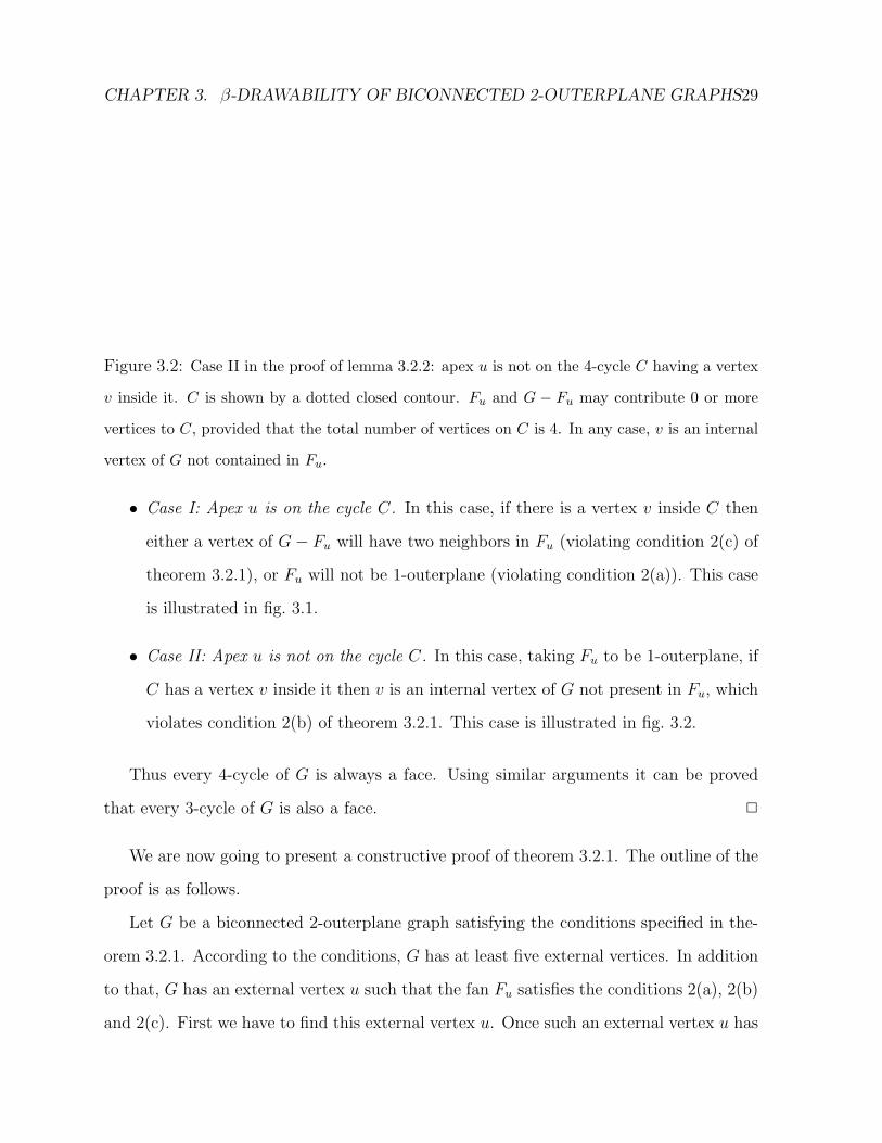
Figure 3.2: Case II in the proof of lemma 3.2.2: apex u is not on the 4-cycle C having a vertex
v inside it. C is shown by a dotted closed contour. Fu and G − Fu may contribute 0 or more
vertices to C, provided that the total number of vertices on C is 4. In any case, v is an internal
vertex of G not contained in Fu.
• Case I: Apex u is on the cycle C. In this case, if there is a vertex v inside C then
either a vertex of G− Fu will have two neighbors in Fu (violating condition 2(c) of
theorem 3.2.1), or Fu will not be 1-outerplane (violating condition 2(a)). This case
is illustrated in fig. 3.1.
• Case II: Apex u is not on the cycle C. In this case, taking Fu to be 1-outerplane, if
C has a vertex v inside it then v is an internal vertex of G not present in Fu, which
violates condition 2(b) of theorem 3.2.1. This case is illustrated in fig. 3.2.
Thus every 4-cycle of G is always a face. Using similar arguments it can be proved
that every 3-cycle of G is also a face. 2
We are now going to present a constructive proof of theorem 3.2.1. The outline of the
proof is as follows.
Let G be a biconnected 2-outerplane graph satisfying the conditions specified in the-
orem 3.2.1. According to the conditions, G has at least five external vertices. In addition
to that, G has an external vertex u such that the fan Fu satisfies the conditions 2(a), 2(b)
and 2(c). First we have to find this external vertex u. Once such an external vertex u has
CHAPTER 3. β-DRAWABILITY OF BICONNECTED 2-OUTERPLANE GRAPHS30
been found, then we draw the fan Fu. Next we draw the remaining graph G − (V (Fu))
and add edges between the vertices of Fu and the vertices of G − (V (Fu)). Finally, we
prove the correctness of the drawing procedure.
Finding an appropriate apex
Now, let us see how we can find an external vertex of G such that the corresponding
fan satisfies the required conditions. In the next lemma we give an algorithm that takes
as input a biconnected 2-outerplane graph G that satisfies the conditions stated in theo-
rem 3.2.1 and finds a set of external vertices of G such that for each vertex u in this set,
the corresponding fan Fu satisfies conditions 2(a), 2(b) and 2(c) of theorem 3.2.1. We call
such a set of external vertex the set of candidate apices.
Lemma 3.2.3 Let G be a biconnected 2-outerplane graph satisfying all the conditions
specified in theorem 3.2.1. The set Sa of external vertices u for which Fu satisfies con-
ditions 2(a), 2(b) and 2(c) of theorem 3.2.1 can be found in O(n2) time, where n is the
number of vertices of G.
Proof. The set Sa, which we call the set of candidate apices, can be found by considering
each external vertex of G and including only those external vertices of G into Sa for which
the corresponding fan satisfies the required conditions. For a given external vertex u of
G, verifying whether Fu satisfies the conditions 2(a), 2(b) and 2(c) of theorem 3.2.1 can
be done in O(n). Thus, if we consider each external vertex of G and verify the conditions
then the total time complexity of this procedure becomes O(n2). 2
Next we give an algorithm named FindApex, that takes a biconnected 2-outerplane
graph satisfying the conditions of theorem 3.2.1 as input and outputs the set Sa of can-
didate apices. The algorithm clearly outlines the steps in the proof of lemma 3.2.3. For
each external vertex u, the algorithm checks whether the fan Fu satisfies all the required
conditions: whether a vertex of the fan has at most one neighbor outside the fan, whether
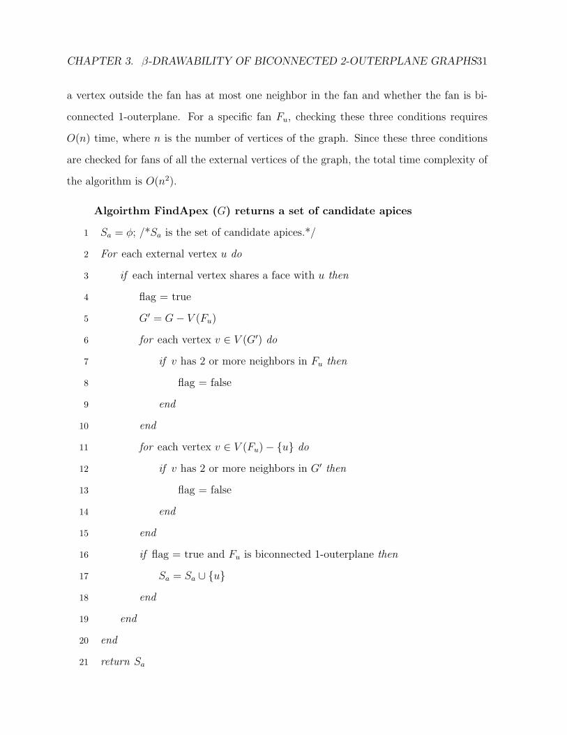
CHAPTER 3. β-DRAWABILITY OF BICONNECTED 2-OUTERPLANE GRAPHS31
a vertex outside the fan has at most one neighbor in the fan and whether the fan is bi-
connected 1-outerplane. For a specific fan Fu, checking these three conditions requires
O(n) time, where n is the number of vertices of the graph. Since these three conditions
are checked for fans of all the external vertices of the graph, the total time complexity of
the algorithm is O(n2).
Algoirthm FindApex (G) returns a set of candidate apices
1 Sa = φ; /*Sa is the set of candidate apices.*/
2 For each external vertex u do
3 if each internal vertex shares a face with u then
4 flag = true
5 G′ = G− V (Fu)
6 for each vertex v ∈ V (G′) do
7 if v has 2 or more neighbors in Fu then
8 flag = false
9 end
10 end
11 for each vertex v ∈ V (Fu)− u do
12 if v has 2 or more neighbors in G′ then
13 flag = false
14 end
15 end
16 if flag = true and Fu is biconnected 1-outerplane then
17 Sa = Sa ∪ u
18 end
19 end
20 end
21 return Sa
CHAPTER 3. β-DRAWABILITY OF BICONNECTED 2-OUTERPLANE GRAPHS32
Drawing the fan
We can obtain a set Sa of candidate apices using the algorithm FindApex stated in
lemma 3.2.3. We can choose any apex from this set for the purpose of β-drawing of the
graph. In the next two lemmas we show how we can β-draw the fan Fu corresponding to
an apex u ∈ Sa. These two lemmas are due to Lenhart and Liotta [LL96]. Lemma 3.2.4
specifies a useful result on how to union two β-drawings so that the resulting drawing
maintains the proximity constraints. We change lemma 3.2.5 slightly from the original
lemma given in [LL96] to fit our purpose.
Lemma 3.2.4 [LL96] Let G1 and G2 be two planar embedded graphs whose intersection
consists of a single edge uv, where u and v lie on the external face of both G1 and G2. Let
Γ1 and Γ2 be embedding-preserving β-drawings of G1 and G2 respectively, for 1 < β < 2.
If Γ1 ∪ Γ2 lies in a convex region having Γ1 and Γ2 on opposite sides of the edge uv then
Γ1 ∪ Γ2 is a β-drawing of G1 ∪G2.
Lemma 3.2.5 [LL96] Let Fu be a biconnected outerplane fan with apex u. Fu can be
β-drawn inside a triangle ∆abc, for β ∈ (1, 2), ∠abc > π2
and ∠bac < π4. Furthermore,
this drawing has the property that the fan edges form a convex chain such that for any
three vertices v1, v2 and v3 on the chain in clockwise order, ∠v1v2v3 > π2.
Proof. The statement can be proved constructively by induction on the number of
neighbors of u.
Base Case: u has exactly two neighbors u1 and u2
Suppose that the two neighbors of u are connected by the chain of nonneighbors of
u: u1,1, u1,2, . . . , u1,m. In this case Fu can be β-drawn by the following procedure (for
illustration please see fig. 3.3):
First, u is placed at the point a of ∆abc and u1 at the point b. Then a straight-line ux
is computed such that ∠u1ux ≤ ∠bac. The line ux intersects the curve Cu,u1,β at the point
CHAPTER 3. β-DRAWABILITY OF BICONNECTED 2-OUTERPLANE GRAPHS33
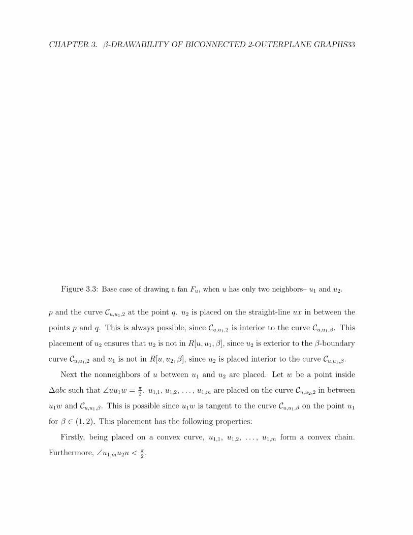
Figure 3.3: Base case of drawing a fan Fu, when u has only two neighbors– u1 and u2.
p and the curve Cu,u1,2 at the point q. u2 is placed on the straight-line ux in between the
points p and q. This is always possible, since Cu,u1,2 is interior to the curve Cu,u1,β. This
placement of u2 ensures that u2 is not in R[u, u1, β], since u2 is exterior to the β-boundary
curve Cu,u1,2 and u1 is not in R[u, u2, β], since u2 is placed interior to the curve Cu,u1,β.
Next the nonneighbors of u between u1 and u2 are placed. Let w be a point inside
∆abc such that ∠uu1w = π2. u1,1, u1,2, . . . , u1,m are placed on the curve Cu,u2,2 in between
u1w and Cu,u1,β. This is possible since u1w is tangent to the curve Cu,u1,β on the point u1
for β ∈ (1, 2). This placement has the following properties:
Firstly, being placed on a convex curve, u1,1, u1,2, . . . , u1,m form a convex chain.
Furthermore, ∠u1,mu2u < π2.
CHAPTER 3. β-DRAWABILITY OF BICONNECTED 2-OUTERPLANE GRAPHS34
Secondly, since u and u1,i are nonadjacent for 1 ≤ i ≤ m, there must be at least one
vertex in R[u, u1,i, β]. We find that u1,i, for 1 ≤ i ≤ m, is exterior to the curve Cu,u1,β. So
u1 is inside R[u, u1,i, β], for 1 ≤ i ≤ m.
Thirdly, since ∠u1u1,iu2 > π2, for 1 ≤ i ≤ m, we can conclude that for any pair of
non-consecutive vertices on the chain, there is an intermediate vertex of the chain in their
β-region.
Thus the statement is proved for the base case.
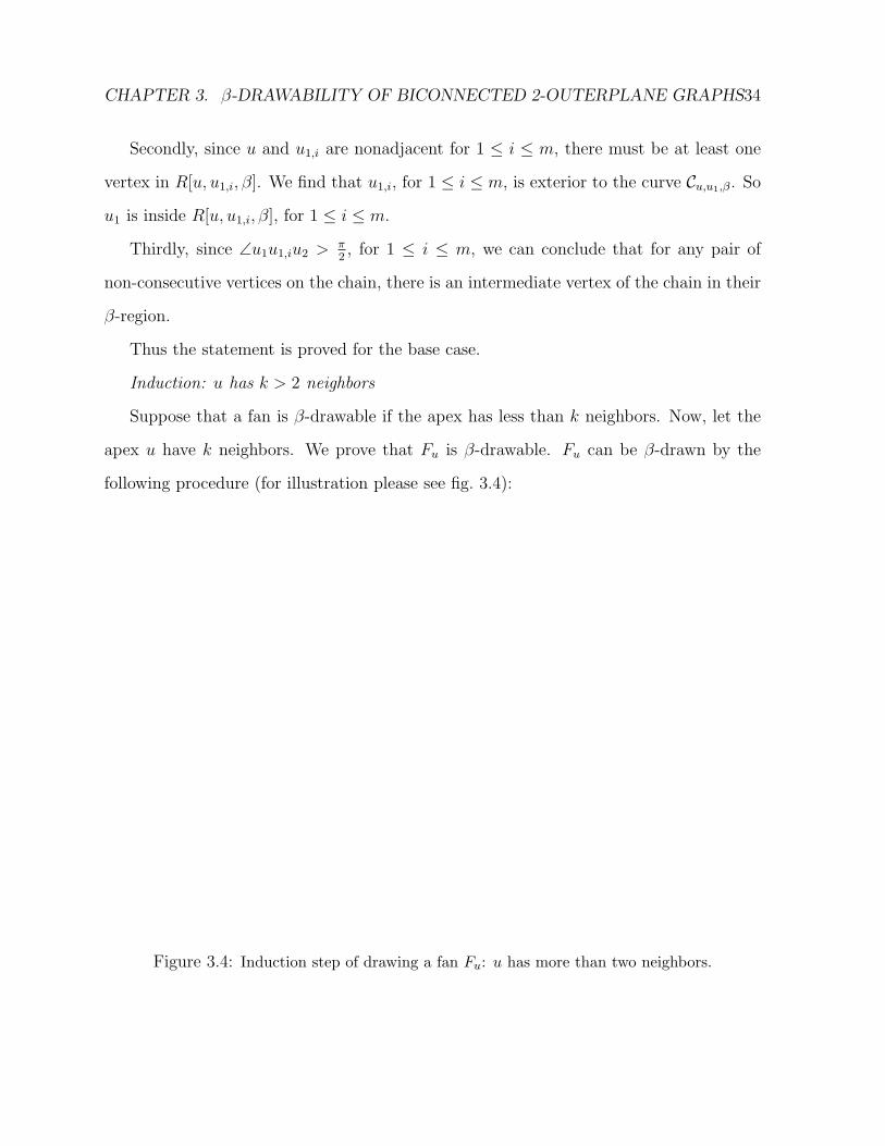
Induction: u has k > 2 neighbors
Suppose that a fan is β-drawable if the apex has less than k neighbors. Now, let the
apex u have k neighbors. We prove that Fu is β-drawable. Fu can be β-drawn by the
following procedure (for illustration please see fig. 3.4):
Figure 3.4: Induction step of drawing a fan Fu: u has more than two neighbors.
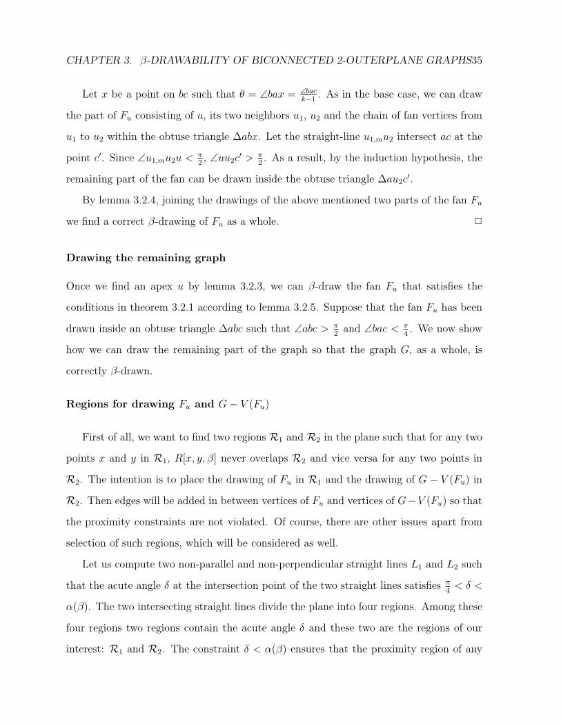
CHAPTER 3. β-DRAWABILITY OF BICONNECTED 2-OUTERPLANE GRAPHS35
Let x be a point on bc such that θ = ∠bax = ∠back−1
. As in the base case, we can draw
the part of Fu consisting of u, its two neighbors u1, u2 and the chain of fan vertices from
u1 to u2 within the obtuse triangle ∆abx. Let the straight-line u1,mu2 intersect ac at the
point c′. Since ∠u1,mu2u < π2, ∠uu2c
′ > π2. As a result, by the induction hypothesis, the
remaining part of the fan can be drawn inside the obtuse triangle ∆au2c′.
By lemma 3.2.4, joining the drawings of the above mentioned two parts of the fan Fu
we find a correct β-drawing of Fu as a whole. 2
Drawing the remaining graph
Once we find an apex u by lemma 3.2.3, we can β-draw the fan Fu that satisfies the
conditions in theorem 3.2.1 according to lemma 3.2.5. Suppose that the fan Fu has been
drawn inside an obtuse triangle ∆abc such that ∠abc > π2
and ∠bac < π4. We now show
how we can draw the remaining part of the graph so that the graph G, as a whole, is
correctly β-drawn.
Regions for drawing Fu and G− V (Fu)
First of all, we want to find two regions R1 and R2 in the plane such that for any two
points x and y in R1, R[x, y, β] never overlaps R2 and vice versa for any two points in
R2. The intention is to place the drawing of Fu in R1 and the drawing of G− V (Fu) in
R2. Then edges will be added in between vertices of Fu and vertices of G−V (Fu) so that
the proximity constraints are not violated. Of course, there are other issues apart from
selection of such regions, which will be considered as well.
Let us compute two non-parallel and non-perpendicular straight lines L1 and L2 such
that the acute angle δ at the intersection point of the two straight lines satisfies π4
< δ <
α(β). The two intersecting straight lines divide the plane into four regions. Among these
four regions two regions contain the acute angle δ and these two are the regions of our
interest: R1 and R2. The constraint δ < α(β) ensures that the proximity region of any
CHAPTER 3. β-DRAWABILITY OF BICONNECTED 2-OUTERPLANE GRAPHS36
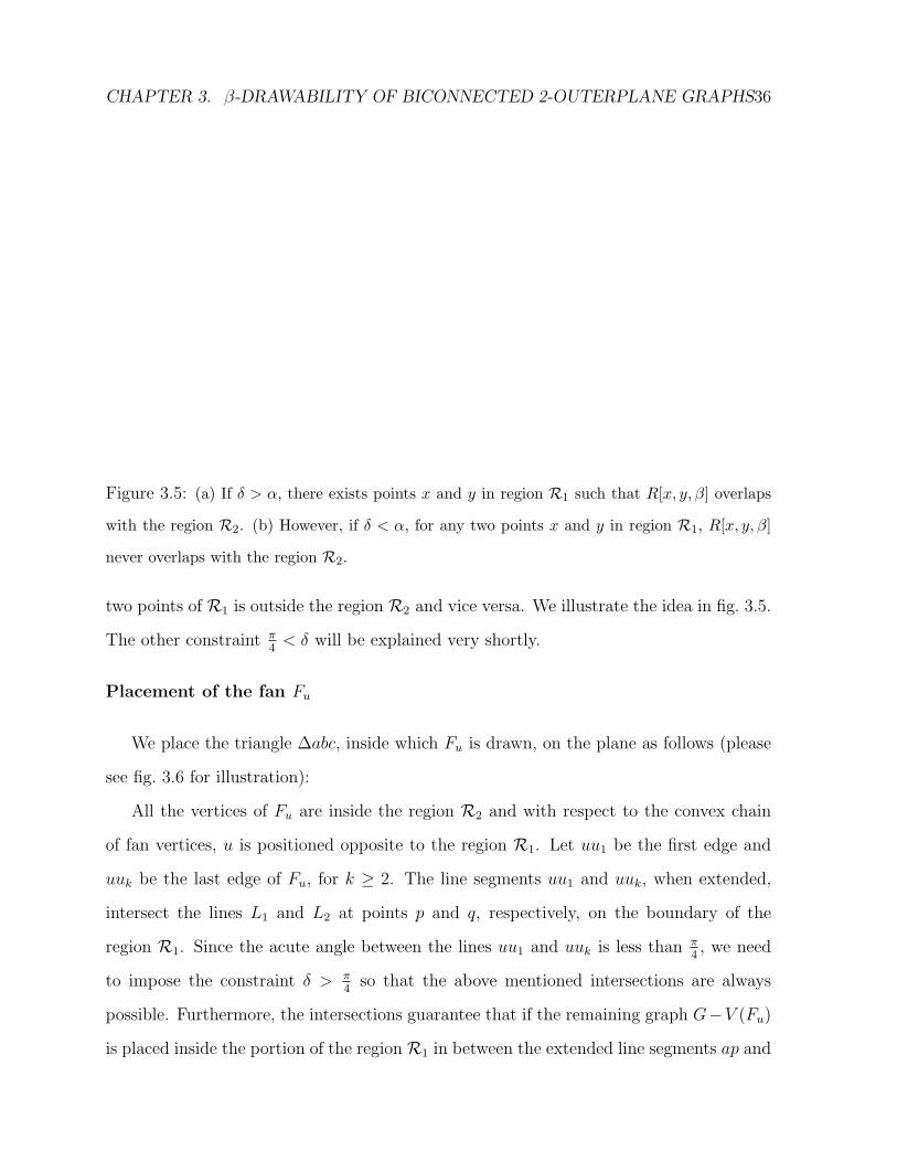
Figure 3.5: (a) If δ > α, there exists points x and y in region R1 such that R[x, y, β] overlaps
with the region R2. (b) However, if δ < α, for any two points x and y in region R1, R[x, y, β]
never overlaps with the region R2.
two points of R1 is outside the region R2 and vice versa. We illustrate the idea in fig. 3.5.
The other constraint π4
< δ will be explained very shortly.
Placement of the fan Fu
We place the triangle ∆abc, inside which Fu is drawn, on the plane as follows (please
see fig. 3.6 for illustration):
All the vertices of Fu are inside the region R2 and with respect to the convex chain
of fan vertices, u is positioned opposite to the region R1. Let uu1 be the first edge and
uuk be the last edge of Fu, for k ≥ 2. The line segments uu1 and uuk, when extended,
intersect the lines L1 and L2 at points p and q, respectively, on the boundary of the
region R1. Since the acute angle between the lines uu1 and uuk is less than π4, we need
to impose the constraint δ > π4
so that the above mentioned intersections are always
possible. Furthermore, the intersections guarantee that if the remaining graph G−V (Fu)
is placed inside the portion of the region R1 in between the extended line segments ap and
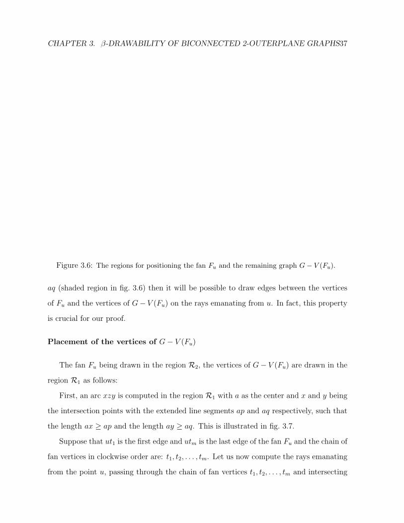
CHAPTER 3. β-DRAWABILITY OF BICONNECTED 2-OUTERPLANE GRAPHS37
Figure 3.6: The regions for positioning the fan Fu and the remaining graph G− V (Fu).
aq (shaded region in fig. 3.6) then it will be possible to draw edges between the vertices
of Fu and the vertices of G− V (Fu) on the rays emanating from u. In fact, this property
is crucial for our proof.
Placement of the vertices of G− V (Fu)
The fan Fu being drawn in the region R2, the vertices of G− V (Fu) are drawn in the
region R1 as follows:
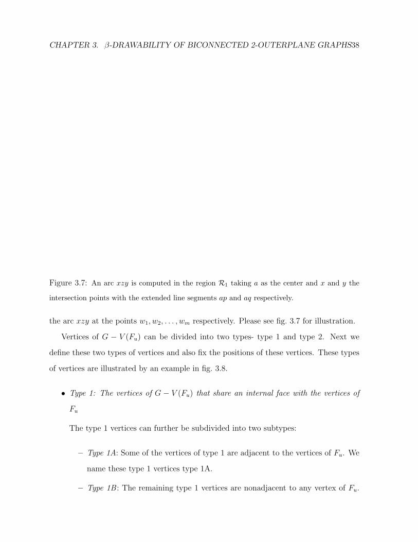
First, an arc xzy is computed in the region R1 with a as the center and x and y being
the intersection points with the extended line segments ap and aq respectively, such that
the length ax ≥ ap and the length ay ≥ aq. This is illustrated in fig. 3.7.
Suppose that ut1 is the first edge and utm is the last edge of the fan Fu and the chain of
fan vertices in clockwise order are: t1, t2, . . . , tm. Let us now compute the rays emanating
from the point u, passing through the chain of fan vertices t1, t2, . . . , tm and intersecting
CHAPTER 3. β-DRAWABILITY OF BICONNECTED 2-OUTERPLANE GRAPHS38
Figure 3.7: An arc xzy is computed in the region R1 taking a as the center and x and y the
intersection points with the extended line segments ap and aq respectively.
the arc xzy at the points w1, w2, . . . , wm respectively. Please see fig. 3.7 for illustration.
Vertices of G − V (Fu) can be divided into two types- type 1 and type 2. Next we
define these two types of vertices and also fix the positions of these vertices. These types
of vertices are illustrated by an example in fig. 3.8.
• Type 1: The vertices of G − V (Fu) that share an internal face with the vertices of
Fu
The type 1 vertices can further be subdivided into two subtypes:
– Type 1A: Some of the vertices of type 1 are adjacent to the vertices of Fu. We
name these type 1 vertices type 1A.
– Type 1B : The remaining type 1 vertices are nonadjacent to any vertex of Fu.
CHAPTER 3. β-DRAWABILITY OF BICONNECTED 2-OUTERPLANE GRAPHS39
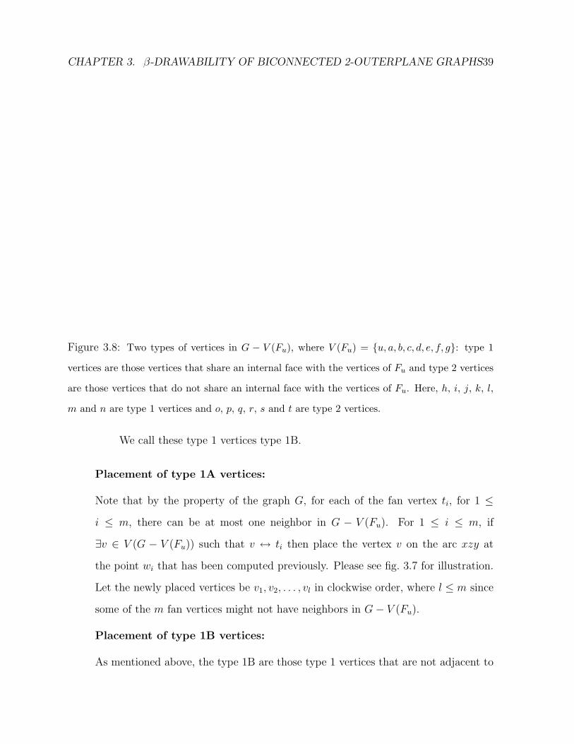
Figure 3.8: Two types of vertices in G − V (Fu), where V (Fu) = u, a, b, c, d, e, f, g: type 1
vertices are those vertices that share an internal face with the vertices of Fu and type 2 vertices
are those vertices that do not share an internal face with the vertices of Fu. Here, h, i, j, k, l,
m and n are type 1 vertices and o, p, q, r, s and t are type 2 vertices.
We call these type 1 vertices type 1B.
Placement of type 1A vertices:
Note that by the property of the graph G, for each of the fan vertex ti, for 1 ≤
i ≤ m, there can be at most one neighbor in G − V (Fu). For 1 ≤ i ≤ m, if
∃v ∈ V (G − V (Fu)) such that v ↔ ti then place the vertex v on the arc xzy at
the point wi that has been computed previously. Please see fig. 3.7 for illustration.
Let the newly placed vertices be v1, v2, . . . , vl in clockwise order, where l ≤ m since
some of the m fan vertices might not have neighbors in G− V (Fu).
Placement of type 1B vertices:
As mentioned above, the type 1B are those type 1 vertices that are not adjacent to

CHAPTER 3. β-DRAWABILITY OF BICONNECTED 2-OUTERPLANE GRAPHS40
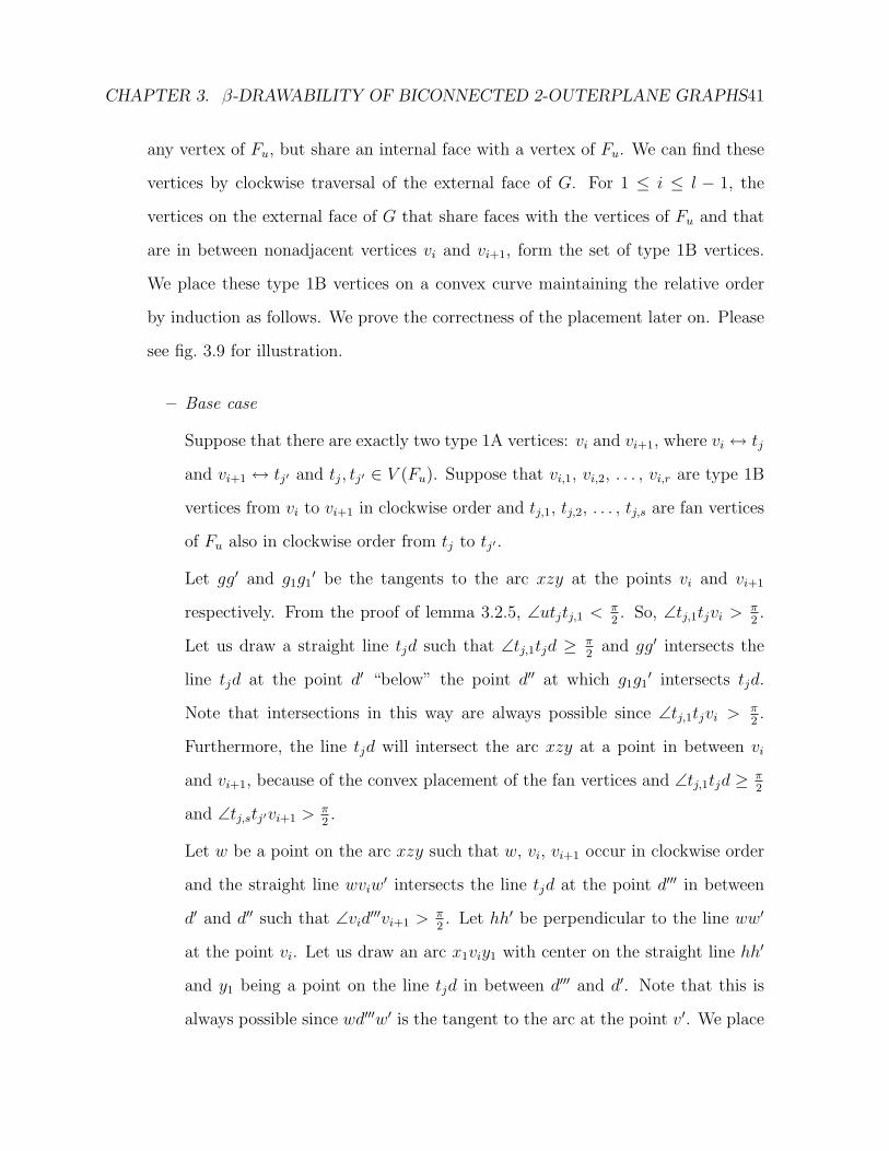
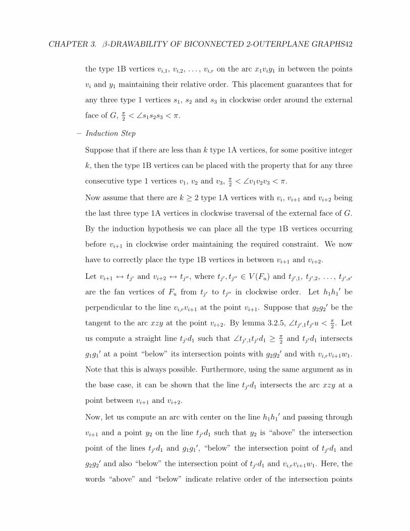
Figure 3.9: Placement of vertices of type 1B.
CHAPTER 3. β-DRAWABILITY OF BICONNECTED 2-OUTERPLANE GRAPHS41
any vertex of Fu, but share an internal face with a vertex of Fu. We can find these
vertices by clockwise traversal of the external face of G. For 1 ≤ i ≤ l − 1, the
vertices on the external face of G that share faces with the vertices of Fu and that
are in between nonadjacent vertices vi and vi+1, form the set of type 1B vertices.
We place these type 1B vertices on a convex curve maintaining the relative order
by induction as follows. We prove the correctness of the placement later on. Please
see fig. 3.9 for illustration.
– Base case
Suppose that there are exactly two type 1A vertices: vi and vi+1, where vi ↔ tj
and vi+1 ↔ tj′ and tj, tj′ ∈ V (Fu). Suppose that vi,1, vi,2, . . . , vi,r are type 1B
vertices from vi to vi+1 in clockwise order and tj,1, tj,2, . . . , tj,s are fan vertices
of Fu also in clockwise order from tj to tj′ .
Let gg′ and g1g1′ be the tangents to the arc xzy at the points vi and vi+1
respectively. From the proof of lemma 3.2.5, ∠utjtj,1 < π2. So, ∠tj,1tjvi > π
2.
Let us draw a straight line tjd such that ∠tj,1tjd ≥ π2
and gg′ intersects the
line tjd at the point d′ “below” the point d′′ at which g1g1′ intersects tjd.
Note that intersections in this way are always possible since ∠tj,1tjvi > π2.
Furthermore, the line tjd will intersect the arc xzy at a point in between vi
and vi+1, because of the convex placement of the fan vertices and ∠tj,1tjd ≥ π2
and ∠tj,stj′vi+1 > π2.
Let w be a point on the arc xzy such that w, vi, vi+1 occur in clockwise order
and the straight line wviw′ intersects the line tjd at the point d′′′ in between
d′ and d′′ such that ∠vid′′′vi+1 > π
2. Let hh′ be perpendicular to the line ww′
at the point vi. Let us draw an arc x1viy1 with center on the straight line hh′
and y1 being a point on the line tjd in between d′′′ and d′. Note that this is
always possible since wd′′′w′ is the tangent to the arc at the point v′. We place
CHAPTER 3. β-DRAWABILITY OF BICONNECTED 2-OUTERPLANE GRAPHS42
the type 1B vertices vi,1, vi,2, . . . , vi,r on the arc x1viy1 in between the points
vi and y1 maintaining their relative order. This placement guarantees that for
any three type 1 vertices s1, s2 and s3 in clockwise order around the external
face of G, π2
< ∠s1s2s3 < π.
– Induction Step
Suppose that if there are less than k type 1A vertices, for some positive integer
k, then the type 1B vertices can be placed with the property that for any three
consecutive type 1 vertices v1, v2 and v3,π2
< ∠v1v2v3 < π.
Now assume that there are k ≥ 2 type 1A vertices with vi, vi+1 and vi+2 being
the last three type 1A vertices in clockwise traversal of the external face of G.
By the induction hypothesis we can place all the type 1B vertices occurring
before vi+1 in clockwise order maintaining the required constraint. We now
have to correctly place the type 1B vertices in between vi+1 and vi+2.
Let vi+1 ↔ tj′ and vi+2 ↔ tj′′ , where tj′ , tj′′ ∈ V (Fu) and tj′,1, tj′,2, . . . , tj′,s′
are the fan vertices of Fu from tj′ to tj′′ in clockwise order. Let h1h1′ be
perpendicular to the line vi,rvi+1 at the point vi+1. Suppose that g2g2′ be the
tangent to the arc xzy at the point vi+2. By lemma 3.2.5, ∠tj′,1tj′u < π2. Let
us compute a straight line tj′d1 such that ∠tj′,1tj′d1 ≥ π2
and tj′d1 intersects
g1g1′ at a point “below” its intersection points with g2g2
′ and with vi,rvi+1w1.
Note that this is always possible. Furthermore, using the same argument as in
the base case, it can be shown that the line tj′d1 intersects the arc xzy at a
point between vi+1 and vi+2.
Now, let us compute an arc with center on the line h1h1′ and passing through
vi+1 and a point y2 on the line tj′d1 such that y2 is “above” the intersection
point of the lines tj′d1 and g1g1′, “below” the intersection point of tj′d1 and
g2g2′ and also “below” the intersection point of tj′d1 and vi,rvi+1w1. Here, the
words “above” and “below” indicate relative order of the intersection points
CHAPTER 3. β-DRAWABILITY OF BICONNECTED 2-OUTERPLANE GRAPHS43
on the line tj′d1 with respect to u.
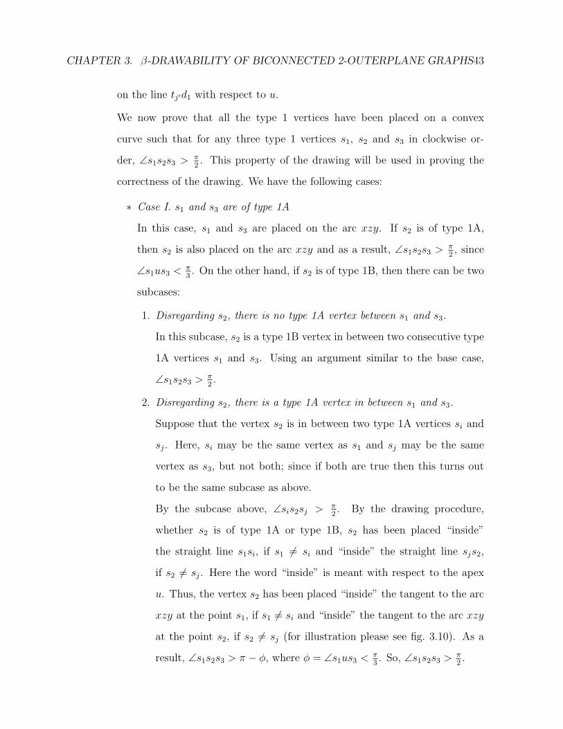
We now prove that all the type 1 vertices have been placed on a convex
curve such that for any three type 1 vertices s1, s2 and s3 in clockwise or-
der, ∠s1s2s3 > π2. This property of the drawing will be used in proving the
correctness of the drawing. We have the following cases:
∗ Case I. s1 and s3 are of type 1A
In this case, s1 and s3 are placed on the arc xzy. If s2 is of type 1A,
then s2 is also placed on the arc xzy and as a result, ∠s1s2s3 > π2, since
∠s1us3 < π3. On the other hand, if s2 is of type 1B, then there can be two
subcases:
1. Disregarding s2, there is no type 1A vertex between s1 and s3.
In this subcase, s2 is a type 1B vertex in between two consecutive type
1A vertices s1 and s3. Using an argument similar to the base case,
∠s1s2s3 > π2.
2. Disregarding s2, there is a type 1A vertex in between s1 and s3.
Suppose that the vertex s2 is in between two type 1A vertices si and
sj. Here, si may be the same vertex as s1 and sj may be the same
vertex as s3, but not both; since if both are true then this turns out
to be the same subcase as above.
By the subcase above, ∠sis2sj > π2. By the drawing procedure,
whether s2 is of type 1A or type 1B, s2 has been placed “inside”
the straight line s1si, if s1 6= si and “inside” the straight line sjs2,
if s2 6= sj. Here the word “inside” is meant with respect to the apex
u. Thus, the vertex s2 has been placed “inside” the tangent to the arc
xzy at the point s1, if s1 6= si and “inside” the tangent to the arc xzy
at the point s2, if s2 6= sj (for illustration please see fig. 3.10). As a
result, ∠s1s2s3 > π − φ, where φ = ∠s1us3 < π3. So, ∠s1s2s3 > π
2.
CHAPTER 3. β-DRAWABILITY OF BICONNECTED 2-OUTERPLANE GRAPHS44
Figure 3.10: The internal angle between three type 1 vertices
∗ Case II. s1 or s3 or both are of type 1B
We have to prove that ∠s1s2s3 > π2. We have the following subcases:
1. s1 is of type 1B and s3 is of type 1A
s1 is placed “above” the arc xzy and s3 is placed on this arc. Let us1
intersect the curve xzy at the point r. Thus using the same argument as
in case I, ∠rs2s3 > π2, which implies that ∠s1s2s3 > π
2.
2. s1 is of type 1A and s3 is of type 1B
This subcase is symmetric to the previous subcase.
3. Both s1 and s3 are of type 1B
Let us1 intersect the curve xzy at the point r1 and us3 intersect the curve
xzy at the point r2. By the same argument as in case I, ∠r1s2r2 > π2,
which implies that ∠s1s2s3 > π2.
• Type 2: The vertices of G−V (Fu) that do not share an internal face with any vertex
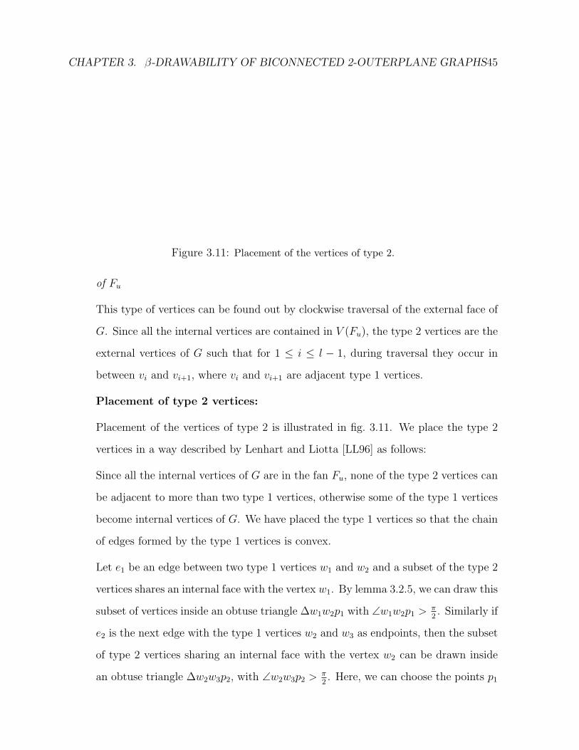
CHAPTER 3. β-DRAWABILITY OF BICONNECTED 2-OUTERPLANE GRAPHS45
Figure 3.11: Placement of the vertices of type 2.
of Fu
This type of vertices can be found out by clockwise traversal of the external face of
G. Since all the internal vertices are contained in V (Fu), the type 2 vertices are the
external vertices of G such that for 1 ≤ i ≤ l − 1, during traversal they occur in
between vi and vi+1, where vi and vi+1 are adjacent type 1 vertices.
Placement of type 2 vertices:
Placement of the vertices of type 2 is illustrated in fig. 3.11. We place the type 2
vertices in a way described by Lenhart and Liotta [LL96] as follows:
Since all the internal vertices of G are in the fan Fu, none of the type 2 vertices can
be adjacent to more than two type 1 vertices, otherwise some of the type 1 vertices
become internal vertices of G. We have placed the type 1 vertices so that the chain
of edges formed by the type 1 vertices is convex.
Let e1 be an edge between two type 1 vertices w1 and w2 and a subset of the type 2
vertices shares an internal face with the vertex w1. By lemma 3.2.5, we can draw this
subset of vertices inside an obtuse triangle ∆w1w2p1 with ∠w1w2p1 > π2. Similarly if
e2 is the next edge with the type 1 vertices w2 and w3 as endpoints, then the subset
of type 2 vertices sharing an internal face with the vertex w2 can be drawn inside
an obtuse triangle ∆w2w3p2, with ∠w2w3p2 > π2. Here, we can choose the points p1
CHAPTER 3. β-DRAWABILITY OF BICONNECTED 2-OUTERPLANE GRAPHS46
and p2 such that ∠w1w2p1 > π2
and ∠p1w2p2 > π2, since every external angle on the
chain of type 1 vertices is greater than π because of convexity.
We perform the placement of type 2 vertices recursively until all of them have been
placed.
Proof of proximity constraints
Let us investigate whether the proximity constraints are satisfied for any two vertices of
G. We have the following cases.
1. Proximity constraints for any two vertices of Fu
By lemma 3.2.5, the fan Fu is correctly β-drawn inside an obtuse triangle. Further-
more, by the selection of the regions for drawing Fu and G− V (Fu), the proximity
region of two adjacent vertices of Fu does not contain any vertex of G− V (Fu).
2. Proximity constraints for any two vertices of type 1
We have three subcases. These are as follows:
(a) Proximity constraints for any two vertices of type 1A
• β-region of two nonadjacent type 1A vertices contains at least another ver-
tex.
Let v1 and v2 be two nonadjacent type 1A vertices. As a result, on the
chain of type 1 vertices, there is another vertex r in between v1 and v2.
This intermediate vertex r is either a type 1A vertex or a type 1B vertex.
First, suppose that r is a type 1A vertex. The vertices of type 1A have
been placed on an arc centered at the apex u such that ∠v1uv2 < δ < π2.
As a result, for any three type 1A vertices v1, r and v2, where v1, r and
v2 occur in clockwise order on the external face of G, ∠v1rv2 > π2. So,
r ∈ R[v1, v2, 1], which implies that r ∈ R[v1, v2, β], for 1 < β < 2.
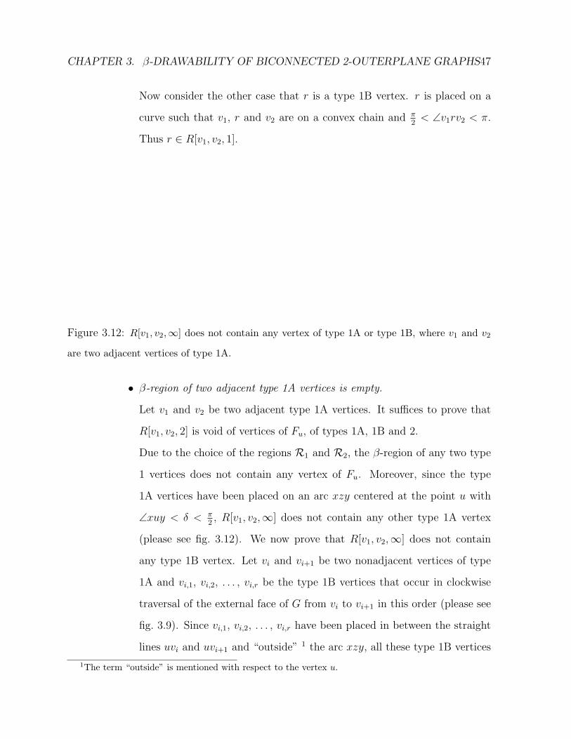
CHAPTER 3. β-DRAWABILITY OF BICONNECTED 2-OUTERPLANE GRAPHS47
Now consider the other case that r is a type 1B vertex. r is placed on a
curve such that v1, r and v2 are on a convex chain and π2
< ∠v1rv2 < π.
Thus r ∈ R[v1, v2, 1].
Figure 3.12: R[v1, v2,∞] does not contain any vertex of type 1A or type 1B, where v1 and v2
are two adjacent vertices of type 1A.
• β-region of two adjacent type 1A vertices is empty.
Let v1 and v2 be two adjacent type 1A vertices. It suffices to prove that
R[v1, v2, 2] is void of vertices of Fu, of types 1A, 1B and 2.
Due to the choice of the regions R1 and R2, the β-region of any two type
1 vertices does not contain any vertex of Fu. Moreover, since the type
1A vertices have been placed on an arc xzy centered at the point u with
∠xuy < δ < π2, R[v1, v2,∞] does not contain any other type 1A vertex
(please see fig. 3.12). We now prove that R[v1, v2,∞] does not contain
any type 1B vertex. Let vi and vi+1 be two nonadjacent vertices of type
1A and vi,1, vi,2, . . . , vi,r be the type 1B vertices that occur in clockwise
traversal of the external face of G from vi to vi+1 in this order (please see
fig. 3.9). Since vi,1, vi,2, . . . , vi,r have been placed in between the straight
lines uvi and uvi+1 and “outside” 1 the arc xzy, all these type 1B vertices
1The term “outside” is mentioned with respect to the vertex u.
CHAPTER 3. β-DRAWABILITY OF BICONNECTED 2-OUTERPLANE GRAPHS48
are outside R[v1, v2,∞]. This is illustrated in fig. 3.12.
Figure 3.13: R[v1, v2, β] does not contain any vertex of type 2.
We now prove that R[v1, v2, β] does not contain any vertex of type 2.
This proof is illustrated in fig. 3.13. The vertices of type 2 have been
placed inside obtuse triangles according to lemma 3.2.5. So, the type 2 ver-
tices that have been placed inside the obtuse triangle ∆v1v2p2 are outside
R[v1, v2, β]. Furthermore, since ∠p1v1p2 > π2
by the drawing procedure,
hence ∠p1v1v2 > π2. So, the type 2 vertices that have been placed inside
∆w1v1p1 are outside R[v1, v2,∞]. Thus, all the type 2 vertices occuring
before v1 in clockwise traversal around the external face of G are outside
R[v1, v2,∞]. By similar argument, the same can be shown for all the type
2 vertices occuring after v2 in clockwise traversal of the external face of G.
This concludes the proof that R[v1, v2, β] does not contain any vertex of
type 2.
(b) Proximity constraints for any two vertices of type 1B
• β-region of two nonadjacent type 1B vertices contains at least another ver-
tex.
Let v1 and v2 be two nonadjacent vertices of type 1B. So, there is an
CHAPTER 3. β-DRAWABILITY OF BICONNECTED 2-OUTERPLANE GRAPHS49
intermediate vertex vi of either type 1A or type 1B. As proved earlier,
∠v1viv2 > π2. Thus the statement follows.
• β-region of two adjacent type 1B vertices is empty.
Let v1 and v2 be two adjacent type 1B vertices. By the same argument
used in proving that the β-region of two adjacent type 1A vertices is empty,
we can show that R[v1, v2, β] is devoid of any vertex of Fu and of type 2.
Now it remains to be shown that R[v1, v2, β] does not contain vertices of
type 1A and type 1B, other than v1 and v2 themselves.
We have already shown that the vertices of type 1 form a convex polytope
with the property that for any three vertices of type 1 in clockwise order,
the internal angle is greater than π2
and less than π. Thus, R[v1, v2,∞]
does not contain any vertex of type 1.
(c) Proximity constraints between a type 1A vertex and a type 1B vertex
Let v1 be a type 1A vertex and v2 be a type 1B vertex. Using similar arguments
as above, it can be shown that if v1 ↔ v2 then R[v1, v2, β] is empty, else
R[v1, v2, 1] contains the type 1 vertices in between v1 and v2.
3. Proximity constraints for any two vertices of type 2
• β-region of two nonadjacent type 2 vertices contains at least another vertex.
Please see fig. 3.11 for illustration of the proof. Suppose that e1 is an edge
between two type 1 vertices w1 and w2. The type 2 vertices that share internal
faces with the vertex w1 have been placed on an obtuse triangle ∆w1w2p1 such
that ∠w1w2p1 > π2. Similarly if e2 is the next edge with the type 1 vertices
w2 and w3 as endpoints, then the of type 2 vertices sharing an internal face
with the vertex w2 have been drawn inside an obtuse triangle ∆w2w3p2, with
∠w2w3p2 > π2. The points p1 and p2 have been chosen such that ∠p1w2p2 > π
2.
CHAPTER 3. β-DRAWABILITY OF BICONNECTED 2-OUTERPLANE GRAPHS50
First, we prove that for any point x in ∆w1w2p1 and y in ∆w2w3p2, w2 ∈
R[x, y, β]. The statement is proved by the fact that ∠xw2y > π2, since ∠p1w2p2 >
π2
and ∠w1w2w3 > π2. Next, using similar argument, we can also prove that for
any two obtuse triangles T1 and T2 based on two edges with type 1 vertices as
endpoints, a type 1 vertex w ∈ R[x, y, β], where x and y are inside the triangles
T1 and T2 respectively. Thus the statement follows for this case.
Next, we prove that for two nonadjacent type 2 vertices inside a single obtuse
triangle there exists another vertex in their β-region. This follows immediately
from lemma 3.2.5.
• β-region of two adjacent type 2 vertices is empty.
Here we use arguments similar to those presented above. First, the region for
drawing type 2 vertices has been chosen such that the β-region of any two type
2 vertices does not contain any vertex of Fu. Let v1 and v2 be two adjacent
type 2 vertices and v1 and v2 be drawn inside an obtuse triangle based on an
edge with two type 1 vertices w1 and w2 as endpoints, where w1 is the apex.
According to lemma 3.2.5, the β-region of v1 and v2 does not contain w1, w2
and any type 2 vertex inside the same triangle. Now it suffices to prove that
R[v1, v2, β] does not contain any type 1 or type 2 vertex outside the triangle in
which v1 and v2 are drawn. The illustration for this proof is shown in fig. 3.14
and we use the same notations as used in the description of drawing the type
2 vertices.
By definition, the edge v1v2 is a fan edge of Fw1 . Let v0 be the type 2 vertex
adjacent to w2. Since ∠v0w2p2 > ∠p1w2p2 > π2, any point inside the triangle
∆w2w3p2 is outside R[v0, w2,∞], which is indicated by the parallel line strip in
fig. 3.14. Since the fan edges of Fw1 form a convex chain having the property
that the internal angle of any three vertices on this chain is greater than π2
and
less than π, for any fan edge v1v2 the β-region of v1 and v2 does not contain
CHAPTER 3. β-DRAWABILITY OF BICONNECTED 2-OUTERPLANE GRAPHS51
Figure 3.14: β-region of two adjacent type 2 vertices v1 and v2 is empty.
any point of ∆w2w3p2.
Now, let us consider the points of ∆w0w1p0. For any two points x and y inside
∆w1w2p1, R[x, y, 2] does not contain any point of ∆w0w1p0. This is because
∠p0w1p1 > π2
and ∠w0w1w2 > π2. Thus an arc with center at x or at y and
with radius xy does not pass through triangle ∆w0w1p0 and the intersection of
these two arcs does not overlap with ∆w0w1p0.
Thus, R[v1, v2, β] does not contain any type 1 or type 2 vertex outside the
triangle in which v1 and v2 are drawn.
4. Proximity constraints for a vertex of Fu and another of type 1
• β-region of a vertex of Fu and another of type 1 that are nonadjacent contains
at least another vertex
For illustration of the proof please see fig. 3.9.
Let us first consider the case of a type 1A vertex nonadjacent to a vertex of Fu.
By definition, a type 1A vertex has a neighboring vertex in Fu. For example,
following the illustration in fig. 3.9, the type 1A vertex vi+1 is adjacent to
tj′ ∈ V (Fu). The type 1A vertex vi+1 is placed in such a way that for any
CHAPTER 3. β-DRAWABILITY OF BICONNECTED 2-OUTERPLANE GRAPHS52
vertex v 6= tj′ ∈ V (Fu), ∠vi+1tj′v > π2. Thus R[vi+1, v, 1] contains tj′ . Same is
the case for any type 1A vertex and a nonadjacent vertex of Fu.
Now let us consider the other case; that is the case of type 1B vertex. By
definition, a type 1B vertex has no neighbor in Fu. Let vi+1,1 be a type 1B vertex
which occurs in between two type 1A vertices vi+1 and vi+2 as shown in fig. 3.9.
Here, vi+1 is adjacent to tj′ ∈ V (Fu) and vi+2 is adjacent to tj′′ ∈ V (Fu). Since
vi+1,1 has been placed “above” the tangent g1g′1 to the arc xzy at the point
vi+1, ∠tj′vi+1vi+1,1 > π2
and thus vi+1 ∈ R[tj′ , vi+1,1, 1]. Furthermore, vi+1,1 has
been placed to the “left” of the line tj′d1 which is perpendicular to the line
tj′tj′,1. Thus, for any vertex v ∈ V (Fu) to the “right” of tj′ , ∠vtj′vi+1,1 > π2.
On the other hand, the same is true for any vertex v ∈ V (Fu) to the “left” of
tj′ , since ∠vtj′vi+1 > π2.
Thus, the statement is proved.
• β-region of a vertex of Fu and another of type 1 that are adjacent is empty
For illustration of the proof please see fig. 3.15. By definition, only a vertex of
type 1A can be adjacent to a vertex of Fu.
From lemma 3.2.5 we find that each of the fan vertices of the fan Fu has been
placed on an arc with center at u. Furthermore, the fan vertices form a convex
chain of fan edges such that for any three fan vertices w1, w2 and w3 on the
chain in clockwise order, ∠w1w2w3 > π2. Furthermore, We have placed all the
type 1A vertices on an arc xzy centered at u.
Let v be a type 1A vertex such that v ↔ w2. We show that R[w2, v, 2] is
empty. By lemma 3.2.5, all the fan vertices to the right of w2 have been drawn
“inside” (w.r.t. u) the tangent hh′ to the β-boundary curve Cu,w2,2 at the
point w2. Furthermore, all the fan vertices to the left of w2 have also been
drawn “inside” (w.r.t. u) hh′. If we consider R[w2, v, 2], we find that hh′ is
also tangent to the circle centered at v and having radius vw2, since the β-
CHAPTER 3. β-DRAWABILITY OF BICONNECTED 2-OUTERPLANE GRAPHS53
Figure 3.15: Illustration for the proof that the β-region of a vertex of Fu and another of type
1 that are adjacent is empty.
boundary curve Cu,w2,2 coincides with R[u, w2, 2]. Thus for any vertex v 6= w2
and v ∈ V (Fu), v /∈ R[w2, v, 2]. Furthermore all the other vertices of type 1
and type 2 are also outside R[w2, v, 2]. Thus R[w2, v, 2] is empty, implying that
R[w2, v, β] is also empty.
5. Proximity constraints for a vertex of Fu and another of type 2
By definition, the type 2 vertices are not adjacent to any vertex of Fu. Thus it
suffices to prove that there is at least another vertex in R[s, t, 1], where t ∈ V (Fu)
and s is a type 2 vertex. The illustration for the proof is shown in fig. 3.16.
CHAPTER 3. β-DRAWABILITY OF BICONNECTED 2-OUTERPLANE GRAPHS54
Figure 3.16: Illustration for the proof that there is at least another vertex in the β-region of a
vertex of Fu and another of type 2.
Let us consider an edge e1 = w1w2 on the chain of type 1 vertices. In an obtuse
triangle based on w1w2 we have placed the corresponding type 2 vertices according
to lemma 3.2.5, as illustrated in fig. 3.11. Let s be a type 2 vertex placed inside
the mentioned triangle and t be any vertex of Fu. By lemma 3.2.5, ∠w1sw2 < π2
and by the choice of regions R1 and R2, ∠w1tw2 < α < π3. Now if we consider the
quadrilateral tw1sw2, then we find that ∠tw1s + ∠sw2t > 7π6
. As a result, either
∠tw1s or ∠sw2t is greater than π2, which implies that either w1 or w2 is in R[s, t, 1].
6. Proximity constraints for a vertex of type 1 and a vertex of type 2
Using the illustration of fig. 3.11 it has been shown that the type 2 vertices have
CHAPTER 3. β-DRAWABILITY OF BICONNECTED 2-OUTERPLANE GRAPHS55
been placed inside obtuse triangles recursively following lemma 3.2.5. It has also
been shown that if x and y are two points inside two distinct triangles then R[x, y, 1]
contains at least another point. Furthermore, by lemma 3.2.5, inside each obtuse
triangle the vertices have been correctly placed. Thus if a vertex of type 1 and a ver-
tex of type 2 are adjacent then their β-region is empty; and if they are nonadjacent
then their β-region contains at least another vertex.
3.3 Application
In this section we illustrate a practical application of the studies we have made so far.
The application we provide here is drawn from the domain of wireless sensor networks.
One of the most interesting aspects of a wireless sensor network is the contention between
two conflicting requirements: one is the conservation of battery power and the other is
the dissemination of information. The sensors need to disseminate their information to
other sensors and at the same time need to save their battery power. That is why energy
efficient topology construction is a very important consideration in the field of wireless
sensor networks.
We can model an energy efficient topology in a wireless sensor network by using
parameterized proximity graphs, because one of the underlying features in a proximity
graph is that the group of adjacent vertices tend to stay close together, whereas the group
of nonadjacent vertices tend to stay relatively farther away. In the case of a wireless
sensor network, the same principle works, that is sensors that are near to each other
should communicate with each other and sensors that are relatively farther away from
each other should not communicate with each other since it requires greater power. Next
we show how we can place sensors in a plane when a desired topology is given as input.
Suppose that we are given a biconnected 2-outerplane graph G describing the topology
of sensors in a wireless sensor network. For illustration please see fig. 3.17. We have to
CHAPTER 3. β-DRAWABILITY OF BICONNECTED 2-OUTERPLANE GRAPHS56
Figure 3.17: The biconnected 2-outerplane graph G describing the topology of sensors in
a wireless sensor network.
place the sensors in a plane such that the placement satisfies the proximity constraints
for a given value of β, where 1 < β < 2. This range of β value guarantees that if G is
β-drawable then there will be no edge-crossing in the β-drawing of G, which is practically
desirable. The first question we have is that is the graph G β-drawable for the given
value of β? We have proved that if G satisfies the conditions of theorem 3.2.1 then G is
β-drawable. Suppose that G satisfies the conditions of theorem 3.2.1. Next we have to
draw G maintaining the proximity constraints. The drawing of G shown in fig. 3.17 is
illustrated in fig. 3.18.
Since G satisfies the conditions of theorem 3.2.1, by lemma 3.2.3 we can find an
appropriate apex u ∈ V (G). According to the drawing algorithm given in section 3.2, we
can draw the fan Fu in an obtuse triangle. For the example given in fig. 3.17, the vertices
CHAPTER 3. β-DRAWABILITY OF BICONNECTED 2-OUTERPLANE GRAPHS57
Figure 3.18: Drawing of the biconnected 2-outerplane graph G shown in fig. 3.17.
of Fu are u, a, b, c, d, e, f , g, h and i. The drawing of Fu is placed inside the region R2
as described in section 3.2. Next the remaining graph is drawn in region R1 according to
the drawing algorithm of theorem 3.2.1 and all the edges between the vertices of the fan
CHAPTER 3. β-DRAWABILITY OF BICONNECTED 2-OUTERPLANE GRAPHS58
and the vertices of the remaining graph are drawn.
Finally, we can place the sensors in the real world according to the obtained drawing
of G and scaling the drawing to account for the desired maximum length of an edge.
3.4 Chapter Summary
In this chapter we have concentrated on the problem of β-drawability of a biconnected
2-outerplane graph. We have given a necessary condition and a set of sufficient conditions
for β-drawability of a biconnected 2-outerplane graph. We have proved the sufficient
conditions by construction. This proof method gives us an O(n2) drawing algorithm.
Although the drawing algorithm has a high time complexity, the focus of our work is on
answering the question of β-drawability of a biconnected 2-outerplane graph. In the next
chapter we are going to explore “forbidden” biconnected 2-outerplane graphs, which do
not admit a β-drawing. We are going to identify a subclass of biconnected 2-outerplane
graphs that are forbidden. We are also going to show that if a biconnected 2-outerplane
graph does not satisfy the sufficient conditions, then it is not necessarily β-drawable.
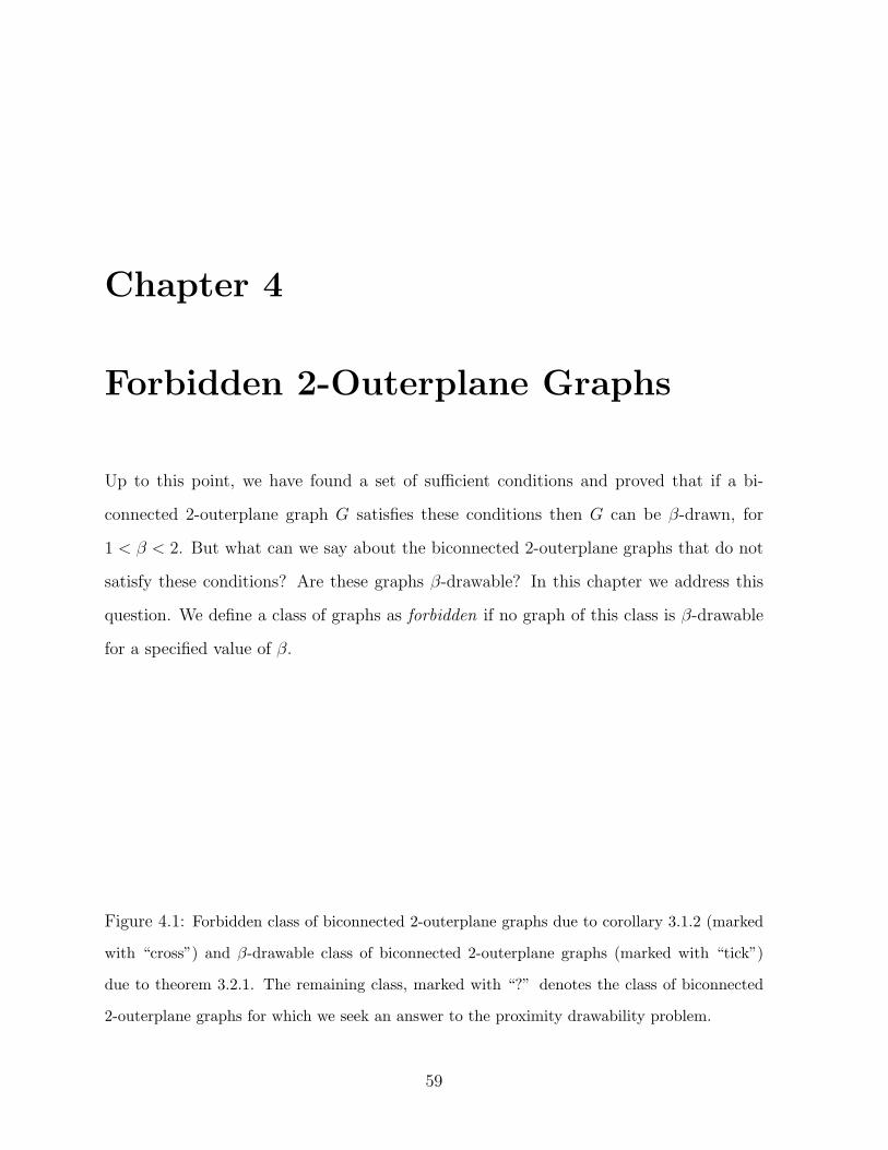
Chapter 4
Forbidden 2-Outerplane Graphs
Up to this point, we have found a set of sufficient conditions and proved that if a bi-
connected 2-outerplane graph G satisfies these conditions then G can be β-drawn, for
1 < β < 2. But what can we say about the biconnected 2-outerplane graphs that do not
satisfy these conditions? Are these graphs β-drawable? In this chapter we address this
question. We define a class of graphs as forbidden if no graph of this class is β-drawable
for a specified value of β.
Figure 4.1: Forbidden class of biconnected 2-outerplane graphs due to corollary 3.1.2 (marked
with “cross”) and β-drawable class of biconnected 2-outerplane graphs (marked with “tick”)
due to theorem 3.2.1. The remaining class, marked with “?” denotes the class of biconnected
2-outerplane graphs for which we seek an answer to the proximity drawability problem.
59
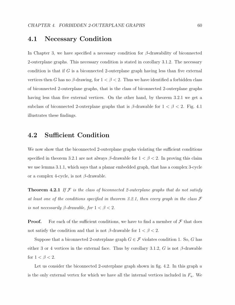
CHAPTER 4. FORBIDDEN 2-OUTERPLANE GRAPHS 60
4.1 Necessary Condition
In Chapter 3, we have specified a necessary condition for β-drawability of biconnected
2-outerplane graphs. This necessary condition is stated in corollary 3.1.2. The necessary
condition is that if G is a biconnected 2-outerplane graph having less than five external
vertices then G has no β-drawing, for 1 < β < 2. Thus we have identified a forbidden class
of biconnected 2-outerplane graphs, that is the class of biconnected 2-outerplane graphs
having less than five external vertices. On the other hand, by theorem 3.2.1 we get a
subclass of biconnected 2-outerplane graphs that is β-drawable for 1 < β < 2. Fig. 4.1
illustrates these findings.
4.2 Sufficient Condition
We now show that the biconnected 2-outerplane graphs violating the sufficient conditions
specified in theorem 3.2.1 are not always β-drawable for 1 < β < 2. In proving this claim
we use lemma 3.1.1, which says that a planar embedded graph, that has a complex 3-cycle
or a complex 4-cycle, is not β-drawable.
Theorem 4.2.1 If F is the class of biconnected 2-outerplane graphs that do not satisfy
at least one of the conditions specified in theorem 3.2.1, then every graph in the class F
is not necessarily β-drawable, for 1 < β < 2.
Proof. For each of the sufficient conditions, we have to find a member of F that does
not satisfy the condition and that is not β-drawable for 1 < β < 2.
Suppose that a biconnected 2-outerplane graph G ∈ F violates condition 1. So, G has
either 3 or 4 vertices in the external face. Thus by corollary 3.1.2, G is not β-drawable
for 1 < β < 2.
Let us consider the biconnected 2-outerplane graph shown in fig. 4.2. In this graph u
is the only external vertex for which we have all the internal vertices included in Fu. We
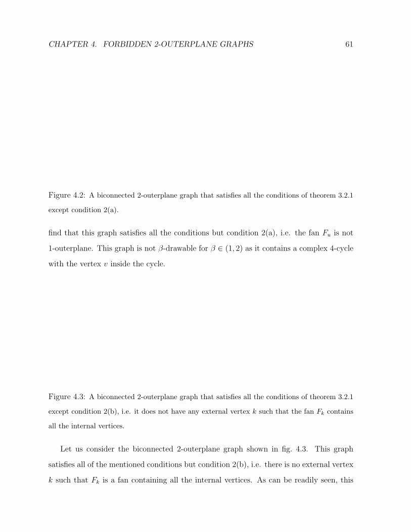
CHAPTER 4. FORBIDDEN 2-OUTERPLANE GRAPHS 61
Figure 4.2: A biconnected 2-outerplane graph that satisfies all the conditions of theorem 3.2.1
except condition 2(a).
find that this graph satisfies all the conditions but condition 2(a), i.e. the fan Fu is not
1-outerplane. This graph is not β-drawable for β ∈ (1, 2) as it contains a complex 4-cycle
with the vertex v inside the cycle.
Figure 4.3: A biconnected 2-outerplane graph that satisfies all the conditions of theorem 3.2.1
except condition 2(b), i.e. it does not have any external vertex k such that the fan Fk contains
all the internal vertices.
Let us consider the biconnected 2-outerplane graph shown in fig. 4.3. This graph
satisfies all of the mentioned conditions but condition 2(b), i.e. there is no external vertex
k such that Fk is a fan containing all the internal vertices. As can be readily seen, this
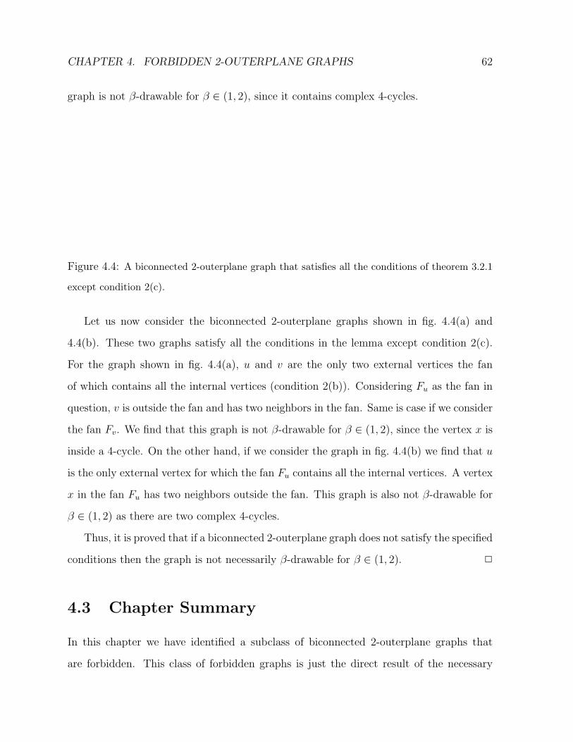
CHAPTER 4. FORBIDDEN 2-OUTERPLANE GRAPHS 62
graph is not β-drawable for β ∈ (1, 2), since it contains complex 4-cycles.
Figure 4.4: A biconnected 2-outerplane graph that satisfies all the conditions of theorem 3.2.1
except condition 2(c).
Let us now consider the biconnected 2-outerplane graphs shown in fig. 4.4(a) and
4.4(b). These two graphs satisfy all the conditions in the lemma except condition 2(c).
For the graph shown in fig. 4.4(a), u and v are the only two external vertices the fan
of which contains all the internal vertices (condition 2(b)). Considering Fu as the fan in
question, v is outside the fan and has two neighbors in the fan. Same is case if we consider
the fan Fv. We find that this graph is not β-drawable for β ∈ (1, 2), since the vertex x is
inside a 4-cycle. On the other hand, if we consider the graph in fig. 4.4(b) we find that u
is the only external vertex for which the fan Fu contains all the internal vertices. A vertex
x in the fan Fu has two neighbors outside the fan. This graph is also not β-drawable for
β ∈ (1, 2) as there are two complex 4-cycles.
Thus, it is proved that if a biconnected 2-outerplane graph does not satisfy the specified
conditions then the graph is not necessarily β-drawable for β ∈ (1, 2). 2
4.3 Chapter Summary
In this chapter we have identified a subclass of biconnected 2-outerplane graphs that
are forbidden. This class of forbidden graphs is just the direct result of the necessary
CHAPTER 4. FORBIDDEN 2-OUTERPLANE GRAPHS 63
condition for β-drawability of a biconnected 2-outerplane graph, that is given in the
previous chapter. We have also explored the graphs that do not belong to the forbidden
class and also do not belong to the β-drawable graph. We have shown that if a biconnected
2-outerplane graph does not satisfy the sufficient conditions, then it is not necessarily β-
drawable. In the next chapter we conclude this thesis with an overview of the results and
a brief discussion on the open problems related to this thesis.
Chapter 5
Conclusion
In this thesis we have studied the β-drawability problem for biconnected 2-outerplane
graphs. The results of the thesis are summarized as follows:
• We have specified a necessary condition for β-drawability of biconnected 2-outerplane
graphs, for 1 < β < 2.
• We have found sufficient conditions for β-drawability of biconnected 2-outerplane
graphs, for 1 < β < 2.
• For a biconnected 2-outerplane graph that satisfies the sufficient conditions, we have
given an O(n2) drawing algorithm for β-drawing the graph, for 1 < β < 2.
• The specified necessary condition implies a forbidden class of biconnected 2-outerplane
graphs which cannot be β-drawn, for 1 < β < 2. The sufficient conditions imply a
subclass of biconnected 2-outerplane graphs that are β-drawable for the same range
of β values. We have proved by showing counter-examples that if a biconnected
2-outerplane graph does not belong to the forbidden class and also not to the above
mentioned β-drawable class, then this graph is not necessarily β-drawable.
We conclude this thesis with the following open problems:
64
CHAPTER 5. CONCLUSION 65
• Complete characterization of biconnected 2-outerplane graphs is yet to be done. In
this problem, one has to provide necessary and sufficient conditions for β-drawability
of a biconnected 2-outerplane graph. Interestingly, complete characterizations of
trees and outerplanar graphs are still open problems as well [BDLL95, LL96].
• β-drawings of biconnected 2-outerplane graphs have been studied in this thesis and
those of trees and outerplanar graphs have been studied in [BDLL95, LL96]. How-
ever, all these studies concern little about the area requirement. Penna and Vocca
report that the existing algorithms, such as those in [BDLL95, LL96], require expo-
nential area [PV04, PV98]. So, β-drawings of trees, outerplanar graphs and bicon-
nected 2-outerplane graphs in polynomial area is an open problem. Interestingly,
nobody still has the answer to the simplest of these problems, i.e. polynomial area
β-drawings of trees for β = 1.
• Characterization of β-drawability of k-outerplane graphs, for any k ≥ 1, will be
a very interesting finding. This is because every planar embedded graph is a k-
outerplane graph, for some value of k ≥ 1. Thus if we are able to find an answer
the question of β-drawability problem for k-outerplane graphs, for any k ≥ 1 and
for some value of β, then given a planar embedded graph we can tell if that graph
can be β-drawn. However, this will be a greatly challenging problem, because even
for the simplest of graphs, such as trees, there are some values of β for which the
answer to the β-drawability problem is not known.
Bibliography
[AM92] P. K. Agarwal and J. Matousek. Relative neighborhood graphs in three dimen-
sions. In Proceedings of 3rd Annual ACM-SIAM Sympozium on Discrete Algo-
rithms, 58-67, 1992.
[BDLL95] P. Bose, G. Di Battista, W. Lenhart and G. Liotta. Proximity constraints and
representable trees. In R. Tamassia and I. G. Tollis, editors, Graph Drawing
(Proceedings of GD ’94), Lecture Notes in Computer Science, Springer-Verlag,
894:340-351, 1995.
[BLL96] P. Bose, W. Lenhart and G. Liotta. Characterizing proximity trees. Algorith-
mica, 16:83-110, 1996.
[BPT92] B. K. Bhattacharya, R. S. Poulsen and G. T. Toussaint. Application of proximity
graphs to editing nearest neighbor decision rules. Technical Report, School of
Computer Science, McGill University, Montreal, 1992.
[CEG90] B. Chazelle, H. Edelsbrunner, L. J. Guibas, J. E. Hershberger, R. Seidel and M.
Sharir. Slimming down by adding; selecting heavily covered points. In Proceed-
ings of 6th Annual Symposium on Computational Geometry, 116-127, 1990.
[CH67] T. M. Cover and P. E. Hart. Nearest neighbor pattern classification. IEEE Trans-
actions on Information Theory, 13(1):21-27, 1967.
66
BIBLIOGRAPHY 67
[CZ05] M. A. Carreira-Perpinan, R. S. Zemel. Proximity graphs for clustering and man-
ifold learning. Advances in Neural Information Processing Systems, MIT Press,
225-232, 2005.
[Devr88] L. P. Devroye. The expected size of some graphs in computational geometry.
Computers and Mathematics with Applications, 15:53-64, 1988.
[DLW96] G. Di Battista, G. Liotta and S. H. Whitesides. The strength of weak proximity.
In F. J. Brandenburg, editor, Graph Drawing (Proceedings of GD ’95), Lecture
Notes in Computer Science, Springer-Verlag, 1027:178-189, 1996.
[GS69] K. R. Gabriel and R.R. Sokal. A new statistical approach to geographic variation
analysis. Systematic Zoology, 18:259-278, 1969.
[JK91] J. W. Jaromczyk and M. Kowaluk. Constructing the relative neighborhood
graph in 3-dimensional Euclidean space. Discrete Applied Mathematics, 31:181-
192, 1991.
[JT92] J. W. Jaromczyk and G. T. Toussaint. Relative neighborhood graphs and their
relatives. Proceedings IEEE, 80(9):1502-1517, 1992.
[KR85] D. G. Kirkpatrick and J. D. Radke. A framework for computational morphology.
In G. T. Toussaint, editor, Computational Geometry, North-Holland, Amster-
dam, 217-248, 1985.
[LCWW03] X. Y. Li, G. Calinescu, P. J. Wan and Y. Wang. Localized delaunay trian-
gulation with application in ad hoc wireless networks. IEEE Transactions on
Parallel and Distributed Systems, 14:1035-1047, 2003.
[Li03] X. Y. Li. Applications of computational geometry in wireless networks. In X.
Cheng, X. Huang and D. Z. Du, editors, Ad Hoc Wireless Networking, Kluwer
Academic Publisher, 2003.
BIBLIOGRAPHY 68
[LL96] W. Lenhart and G. Liotta. Proximity drawings of outerplanar graphs. Technical
Report CS-96-21, Center for Geometric Computing, Deptartment of Computer
Science, Brown University, 1996.
[LSW04] X. Y. Li, I. Stojmenovic and Y. Wang. Partial delaunay triangulation and degree
limited localized bluetooth scatternet formation. IEEE Transactions on Parallel
and Distributed Systems, 15(4):350-361, 2004.
[MS84] D. W. Matula and R. R. Sokal. Properties of Gabriel graphs relevant to geo-
graphic variation research and the clustering of points in the plane. Geographical
Analysis, 12:205-222, 1984.
[PV98] P. Penna and P. Vocca. Proximity drawings of binary trees in polynomial area.
Proceedings of 10th Canadian Conference on Computational Geometry, 116-117,
1998.
[PV04] P. Penna and P. Vocca. Proximity drawings in polynomial area and volume.
Computational Geometry Theory and Applications, 29(2):91-116, 2004.
[SC91] T. -H. Su and R. -C. Chang. On constructing relative neighborhood graphs in
Euclidean k-dimensional spaces. Computing, 46:121-130, 1991.
[Smit89] W. D. Smith. Studies in computational geometry motivated by mesh generation.
PhD Thesis, Princeton University, 1989.
[Supo83] K. J. Supowit. The relative neighborhood graph, with an application to mini-
mum spanning trees. Journal of the ACM, 30:428-448, 1983.
[Tous80] G. T. Toussaint. The relative neighborhood graph of a finite planar set. Pattern
Recognition, 12:261-268, 1980.
BIBLIOGRAPHY 69
[Tous05] G. T. Toussaint. Geometric proximity graphs for improving nearest neighbor
methods in instance-based learning and data mining. International Journal of
Computational Geometry and Applications, 15(2):101-150, 2005.
[Urqu83] R. B. Urquhart. Some properties of the planar Euclidean relative neighborhood
graph. Pattern Recognition Letters, 317-322, 1983.
[Velt92] R. C. Veltkamp. The γ-neighborhood graph. Computational Geometry, Theory
and Applications, 1(4):227-246, 1992.
Index
α(β), 22
β-drawing, 21
β-boundary curve, 24
β-drawability of biconnected 2-outerplane
graphs
necessary condition, 27
sufficient conditions, 27
β-drawability problem, 8
strong, 9
weak, 9
β-drawing
closed, 21
open, 21
β-region, 19, 20
closed, 20
open, 20
γ(β), 22
computational morphology, 5
computer vision, 5
cycle, 14
complex cycle, 18
disconnected graph, 14
external edge, 17
external vertex, 17
fan, 18
apex of, 18
drawing of, 32
fan edge, 18
first edge, 18
last edge, 18
radial edge, 18
forbidden graph, 59
Gabriel graph, 2
Gabriel region, 2
graph, 13
β-drawable, 21
k-connected, 14
k-outerplanar, 17
1-outerplanar, 16
component of, 14
connected, 14
connectivity of, 14
outerplanar, 16
outerplanarity of, 17
70
INDEX 71
planar, 14
plane, 15
graph drawing, 15
straight-line, 15
internal edge, 17
internal vertex, 17
mixed edge, 18
path, 14
proximity drawability problem, 8
proximity graphs, 1
proximity region, 2
regions of influence, 2
separating set, 14
subgraph, 14
induced subgraph, 14