1/24

A Data Driven Method for ComputingQuasipotentials

Bo LinDepartment of Mathematics

Joint work with Qianxiao Li and Weiqing Ren

2/24

Outline

Quasipotential

Proposed methodParameterizationLoss function

Numerical examples3D system with known quasipotentialHigh-d system from discretized PDE

Summary

3/24

Dynamical system

Consider the process xt ∈ Rd modeled by the stochasticdifferential equation (SDE):

dxt = f(xt)dt +√εdWt , t > 0. (1)

I f: force field.I 0 < ε� 1: amplitude of the noise.I Wt : standard Brownian motion.

4/24

Attractor

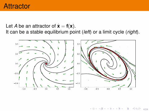
Let A be an attractor of x = f(x).It can be a stable equilibrium point (left) or a limit cycle (right).

5/24

Quasipotential

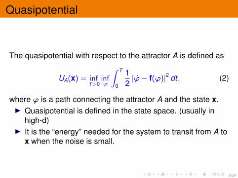
The quasipotential with respect to the attractor A is defined as

UA(x) = infT>0

infϕ

∫ T

0

12|ϕ− f(ϕ)|2 dt , (2)

where ϕ is a path connecting the attractor A and the state x.I Quasipotential is defined in the state space. (usually in

high-d)I It is the “energy” needed for the system to transit from A to

x when the noise is small.

6/24

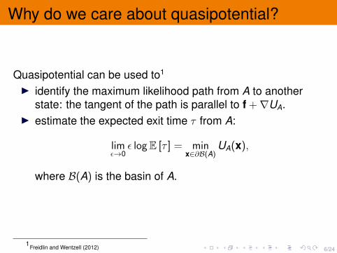
Why do we care about quasipotential?

Quasipotential can be used to1

I identify the maximum likelihood path from A to anotherstate: the tangent of the path is parallel to f +∇UA.

I estimate the expected exit time τ from A:

limε→0

ε logE [τ ] = minx∈∂B(A)

UA(x),

where B(A) is the basin of A.

1Freidlin and Wentzell (2012)

7/24

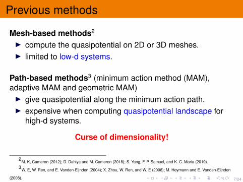
Previous methods

Mesh-based methods2

I compute the quasipotential on 2D or 3D meshes.I limited to low-d systems.

Path-based methods3 (minimum action method (MAM),adaptive MAM and geometric MAM)I give quasipotential along the minimum action path.I expensive when computing quasipotential landscape for

high-d systems.

Curse of dimensionality!

2M. K, Cameron (2012); D. Dahiya and M. Cameron (2018); S. Yang, F. P. Samuel, and K. C. Maria (2019).3W. E, W. Ren, and E. Vanden-Eijnden (2004); X. Zhou, W. Ren, and W. E (2008); M. Heymann and E. Vanden-Eijnden

(2008).

8/24

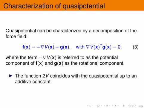
Characterization of quasipotential

Quasipotential can be characterized by a decomposition of theforce field:

f(x) = −∇V (x) + g(x), with ∇V (x)T g(x) = 0, (3)

where the term −∇V (x) is referred to as the potentialcomponent of f(x) and g(x) as the rotational component.

I The function 2V coincides with the quasipotential up to anadditive constant.

9/24

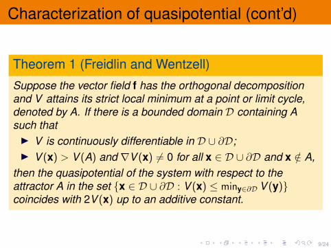
Characterization of quasipotential (cont’d)

Theorem 1 (Freidlin and Wentzell)

Suppose the vector field f has the orthogonal decompositionand V attains its strict local minimum at a point or limit cycle,denoted by A. If there is a bounded domain D containing Asuch thatI V is continuously differentiable in D ∪ ∂D;I V (x) > V (A) and ∇V (x) 6= 0 for all x ∈ D ∪ ∂D and x /∈ A,

then the quasipotential of the system with respect to theattractor A in the set {x ∈ D ∪ ∂D : V (x) ≤ miny∈∂D V (y)}coincides with 2V (x) up to an additive constant.

10/24

Problem setup

Given trajectory data, learn the force field in the form of theorthogonal decomposition.

I The force field f is not explicitly known.I Data-driven: we learn the force field and the quasipotential

from the data.

11/24

Method: Parameterization

Orthogonal decomposition:

f(x) = −∇V (x) + g(x), ∇V (x)T g(x) = 0,

I The two components in the decomposition are representedby neural networks.

12/24

Method: Parameterization (cont’d)

I Parameterization of V :

Vθ(x) = Vθ(x) + |x|2,

Vθ: fully connected neural network with activation tanh.I Parameterization of g by a neural network gθ with

continuously differentiable activation (e.g. tanh(z) orReLU2(z)).

The parameterized force field is given by

fθ(x) = −∇Vθ(x) + gθ(x).

13/24

Method: Trajectory data

The observation dataset

X = {Xi(tj),Xi(tj + ∆t) : i = 1, . . . ,N, j = 0, . . . ,M}

contains N trajectories of the deterministic system

x = f(x)

where Xi(t) denotes the i th trajectory. Along each trajectory,2M + 2 data points are sampled at the times

t0, t0 + ∆t , t1, t1 + ∆t , ..., tM , tM + ∆t ,

where t0 < t1 < ... < tM and ∆t is a small time step.

14/24

Method: Loss function

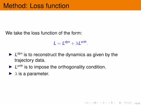
We take the loss function of the form:

L = Ldyn + λLorth.

I Ldyn is to reconstruct the dynamics as given by thetrajectory data.

I Lorth is to impose the orthogonality condition.I λ is a parameter.

15/24

Method: Loss function (cont’d)

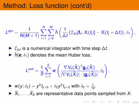
Ldyn =1

N(M + 1)

N∑i=1

M∑j=0

h(

1∆t

(I∆t [fθ; Xi(tj)]− Xi(tj + ∆t)) ; δ1

),

I I∆t is a numerical integrator with time step ∆t .I h(e; δ1) denotes the mean Huber loss.

Lorth =1S

S∑i=1

w

(∇Vθ(Xi)

T gθ(Xi)

|∇Vθ(Xi)| · |gθ(Xi)|; δ2

),

I w(y ; δ2) = y2Iy>0 + δ2y2Iy<0 with δ2 = 110 .

I X1, . . . , XS are representative data points sampled from X .

16/24

Numerical examples

I Adam optimizer and mini-batch of size 5000.I The learning rate exponentially decays.I Two hidden layers in the neural networks.

17/24

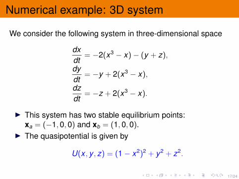
Numerical example: 3D system

We consider the following system in three-dimensional space

dxdt

= −2(x3 − x)− (y + z),

dydt

= −y + 2(x3 − x),

dzdt

= −z + 2(x3 − x).

I This system has two stable equilibrium points:xa = (−1,0,0) and xb = (1,0,0).

I The quasipotential is given by

U(x , y , z) = (1− x2)2 + y2 + z2.

18/24

Numerical example: 3D system

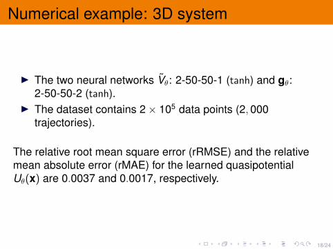
I The two neural networks Vθ: 2-50-50-1 (tanh) and gθ:2-50-50-2 (tanh).

I The dataset contains 2× 105 data points (2,000trajectories).

The relative root mean square error (rRMSE) and the relativemean absolute error (rMAE) for the learned quasipotentialUθ(x) are 0.0037 and 0.0017, respectively.

19/24

Numerical example: 3D system

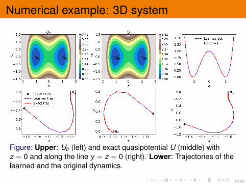
Figure: Upper: Uθ (left) and exact quasipotential U (middle) withz = 0 and along the line y = z = 0 (right). Lower: Trajectories of thelearned and the original dynamics.

20/24

Numerical example: High-d system fromdiscretized PDE

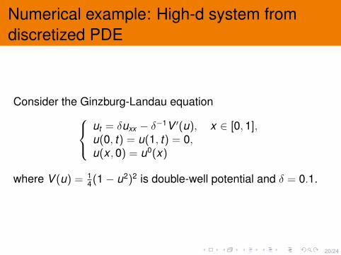
Consider the Ginzburg-Landau equationut = δuxx − δ−1V ′(u), x ∈ [0,1],u(0, t) = u(1, t) = 0,u(x ,0) = u0(x)

where V (u) = 14(1− u2)2 is double-well potential and δ = 0.1.

21/24

Numerical example: High-d system

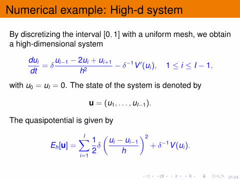
By discretizing the interval [0,1] with a uniform mesh, we obtaina high-dimensional system

dui

dt= δ

ui−1 − 2ui + ui+1

h2 − δ−1V ′(ui), 1 ≤ i ≤ I − 1,

with u0 = uI = 0. The state of the system is denoted by

u = (u1, . . . ,uI−1).

The quasipotential is given by

Eh[u] =I∑

i=1

12δ

(ui − ui−1

h

)2

+ δ−1V (ui).

22/24

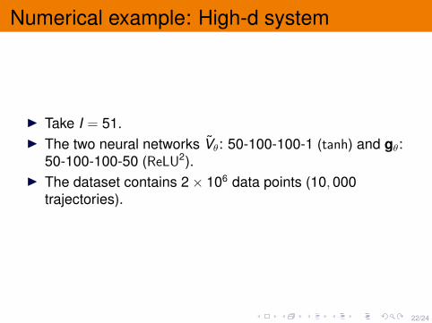
Numerical example: High-d system

I Take I = 51.I The two neural networks Vθ: 50-100-100-1 (tanh) and gθ:

50-100-100-50 (ReLU2).I The dataset contains 2× 106 data points (10,000

trajectories).

23/24

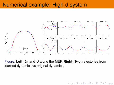
Numerical example: High-d system

Figure: Left: Uθ and U along the MEP. Right: Two trajectories fromlearned dynamics vs original dynamics.

24/24

Summary

I We proposed a method for computing the quasipotentialand at the same time learning the dynamics from thetrajectory data.

I The method is data-driven.I It is an efficient method to map the landscape of the

quasipotential in high dimensions.