Classical Discrete Choice Theoryjenni.uchicago.edu/econ312/Slides/Classic-Discrete... ·...
184
Classical Discrete Choice Theory James J. Heckman University of Chicago Econ 312, Spring 2019 Heckman Classical Discrete Choice Theory
Transcript of Classical Discrete Choice Theoryjenni.uchicago.edu/econ312/Slides/Classic-Discrete... ·...
Classical Discrete Choice Theory
James J. HeckmanUniversity of Chicago
Econ 312, Spring 2019
Heckman Classical Discrete Choice Theory
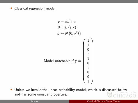
• Classical regression model:
y = xβ + ε
0 = E (ε|x)
E ∼ N(0, σ2I
)
Model untenable if y =
110:10:001
• Unless we invoke the linear probability model, which is discussed below
and has some unusual properties.
Heckman Classical Discrete Choice Theory
• To model discrete choices, need to think of the ingredients thatgive rise to choices.
• For example, suppose we want to forecast demand for a newgood. We observe consumption data on old goods x1...xI .(Each good could represent a transportation mode, forexample, or an occupation choice.)
• Assume people choose a good that yields highest utility. Whenwe have a new good, we need a way of putting it on a basiswith the old.
• Earliest literature on discrete choice was developed inpsychometrics where researchers were concerned with modelingchoice behavior (Thurstone).
• These are also models of counterfactual utilities.
Heckman Classical Discrete Choice Theory
Two dominant modeling approaches
(i) Luce Model (1953) ⇐⇒ McFadden Conditional logit model
(ii) Thurstone-Quandt Model (1929, 1930s). (Multivariateprobit/normal model)
Heckman Classical Discrete Choice Theory

Other approaches
(i) GEV models1 Luce-McFadden Model
• widely used in economics• easy to compute• identifiability of parameters understood• very restrictive substitution possibilities among goods• restrictive heterogeneity• imposes arbitrary preference shocks
2 Quandt-Thurstone Model• very general substitution possibilities• allows for more general forms of heterogeneity• more difficult to compute• identifiability less easily established• does not necessarily rely on preference shocks
Heckman Classical Discrete Choice Theory
Luce Model/McFadden Conditional Logit Model
• References: Manski and McFadden, Chapter 5, Yellot paper
• Notation:• X : universe of objects of choice• S : universe of attributes of persons• B: feasible choice set (x ∈ B ⊆ X )
Heckman Classical Discrete Choice Theory
Luce Model/McFadden Conditional Logit Model
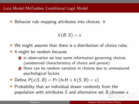
• Behavior rule mapping attributes into choices: h
h (B , S) = x
• We might assume that there is a distribution of choice rules.
• h might be random because
(a) in observation we lose some information governing choices(unobserved characteristics of choice and person)
(b) there can be random variation in choices due to unmeasuredpsychological factors
• Define P(x |S ,B) = Pr hεH 3 h (S ,B) = x• Probability that an individual drawn randomly from the
population with attributes S and alternative set B chooses x .
Heckman Classical Discrete Choice Theory
Luce Axioms
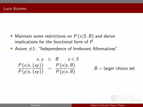
• Maintain some restrictions on P (x |S ,B) and deriveimplications for the functional form of P .
• Axiom #1: “Independence of Irrelevant Alternatives”
x , y ∈ B s ∈ S
P (x |s, xy)P (y |s, xy)
=P (x |s,B)
P (y |s,B)B = larger choice set
Heckman Classical Discrete Choice Theory
Luce Axioms
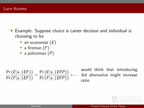
• Example: Suppose choice is career decision and individual ischoosing to be• an economist (E )• a fireman (F )• a policeman (P)
Pr (E |s, EF)Pr (F |s, EF)
=Pr (E |s, EFP)Pr (F |s, EFP)
←−would think that introducing3rd alternative might increaseratio
Heckman Classical Discrete Choice Theory
Luce Axioms
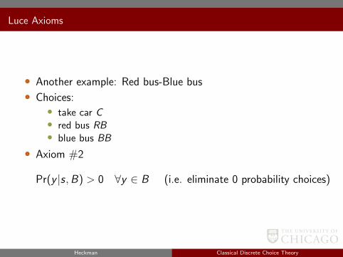
• Another example: Red bus-Blue bus
• Choices:• take car C• red bus RB• blue bus BB
• Axiom #2
Pr(y |s,B) > 0 ∀y ∈ B (i.e. eliminate 0 probability choices)
Heckman Classical Discrete Choice Theory

Implications of above axioms
• Define Pxy = P(x |s, xy)• Assume Pxx = 1
2
P (y |s,B) =Pyx
PxyP (x |s,B) by IIA axiom∑
y∈B
P (y |s,B) = 1 =⇒ P (x |s,B) =1∑
y∈BPyx
Pxy
Heckman Classical Discrete Choice Theory
Implications of above axioms
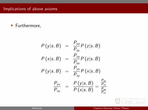
• Furthermore,
P (y |s,B) =Pyz
PzyP (z |s,B)
P (x |s,B) =Pxz
PzxP (z |s,B)
P (y |s,B) =Pyx
PxyP (x |s,B)
Pyx
Pxy=
P (y |s,B)
P (x |s,B)=
Pyz
Pzy
Pxz
Pzx
Heckman Classical Discrete Choice Theory
Implications of above axioms
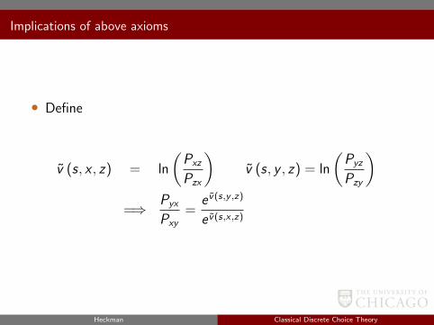
• Define
v (s, x , z) = ln
(Pxz
Pzx
)v (s, y , z) = ln
(Pyz
Pzy
)=⇒ Pyx
Pxy=
e v(s,y ,z)
e v(s,x ,z)
Heckman Classical Discrete Choice Theory
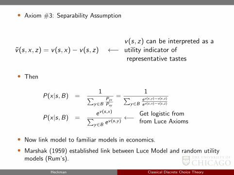
• Axiom #3: Separability Assumption
v(s, x , z) = v(s, x)− v(s, z) ←−v(s, z) can be interpreted as autility indicator ofrepresentative tastes
• Then
P(x |s,B) =1∑
y∈BPyx
Pxy
=1∑
y∈Bev(s,y)−v(s,z)
ev(s,x)−v(s,z)
P(x |s,B) =ev(s,x)∑y∈B ev(s,y)
←− Get logistic fromfrom Luce Axioms
• Now link model to familiar models in economics.
• Marshak (1959) established link between Luce Model and random utilitymodels (Rum’s).
Heckman Classical Discrete Choice Theory
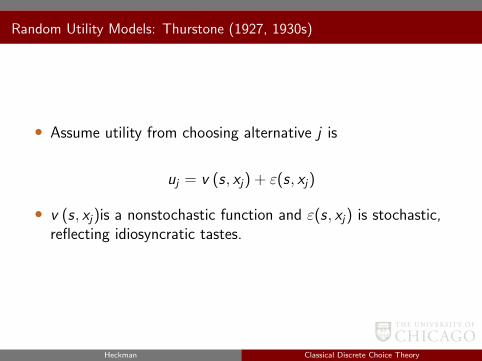
Random Utility Models: Thurstone (1927, 1930s)
• Assume utility from choosing alternative j is
uj = v (s, xj) + ε(s, xj)
• v (s, xj)is a nonstochastic function and ε(s, xj) is stochastic,reflecting idiosyncratic tastes.
Heckman Classical Discrete Choice Theory
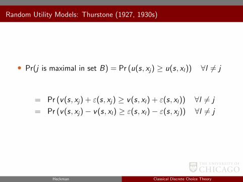
Random Utility Models: Thurstone (1927, 1930s)
• Pr(j is maximal in set B) = Pr (u(s, xj) ≥ u(s, xl)) ∀l 6= j
= Pr (v(s, xj) + ε(s, xj) ≥ v(s, xl) + ε(s, xl)) ∀l 6= j
= Pr (v(s, xj)− v(s, xl) ≥ ε(s, xl)− ε(s, xj)) ∀l 6= j
Heckman Classical Discrete Choice Theory
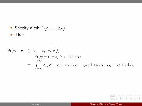
• Specify a cdf F (ε1, ..., εN)
• Then
Pr(vj − vl ≥ εl − εj ∀l 6= j)
= Pr(vj − vl + εj ≥ εl ∀l 6= j)
=
∫ ∞−∞
Fj( vj − v1 + εj , ..., vj − vj−1 + εj , εj , ..., vj − vJ + εj)dεj
Heckman Classical Discrete Choice Theory
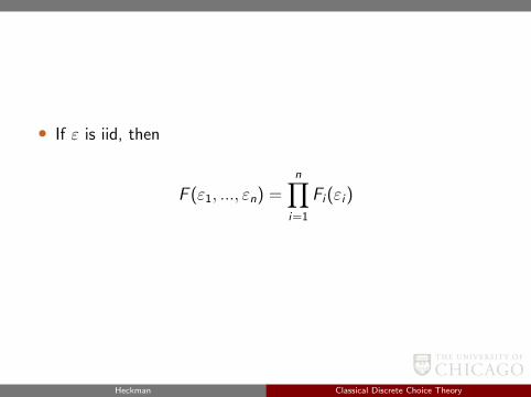
• If ε is iid, then
F (ε1, ..., εn) =n∏
i=1
Fi(εi)
Heckman Classical Discrete Choice Theory
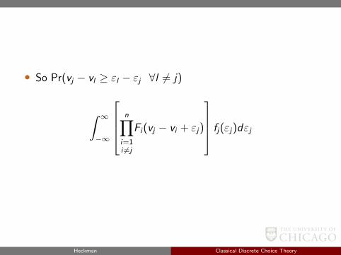
• So Pr(vj − vl ≥ εl − εj ∀l 6= j)
∫ ∞−∞
n∏i=1i 6=j
Fi(vj − vi + εj)
fj(εj)dεj
Heckman Classical Discrete Choice Theory
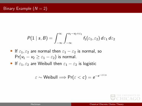
Binary Example (N = 2)
P(1 | s,B) =
∫ ∞−∞
∫ v1−v2+ε1
−∞f1(ε1, ε2) dε1 dε2
• If ε1, ε2 are normal then ε1 − ε2 is normal, soPr(v1 − v2 ≥ ε1 − ε2) is normal.
• If ε1, ε2 are Weibull then ε1 − ε2 is logistic
ε ∼ Weibull =⇒ Pr(ε < c) = e−e−c+α
Heckman Classical Discrete Choice Theory
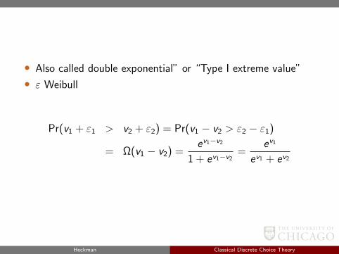
• Also called double exponential” or “Type I extreme value”
• ε Weibull
Pr(v1 + ε1 > v2 + ε2) = Pr(v1 − v2 > ε2 − ε1)
= Ω(v1 − v2) =ev1−v2
1 + ev1−v2=
ev1
ev1 + ev2
Heckman Classical Discrete Choice Theory
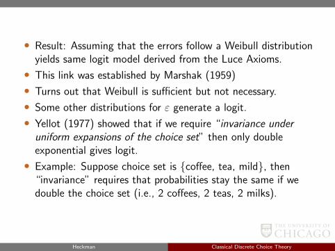
• Result: Assuming that the errors follow a Weibull distributionyields same logit model derived from the Luce Axioms.
• This link was established by Marshak (1959)
• Turns out that Weibull is sufficient but not necessary.
• Some other distributions for ε generate a logit.
• Yellot (1977) showed that if we require “invariance underuniform expansions of the choice set” then only doubleexponential gives logit.
• Example: Suppose choice set is coffee, tea, mild, then“invariance” requires that probabilities stay the same if wedouble the choice set (i.e., 2 coffees, 2 teas, 2 milks).
Heckman Classical Discrete Choice Theory

Some Important Properties of the Weibull
• Developed 1928 (Fisher & Tippet showed it’s one of 3 possiblelimiting distributions for the maximum of a sequence of randomvariables)
• Closed under maximization (i.e. max of n Weibulls is a Weibull)
Pr(maxiεi ≤ c) =
∏i
e−e−(c+α1)
= e−∑i
e−ceαi
= e−e−c∑
i
eαi
= e−e−c+ln
∑i
eαi
Heckman Classical Discrete Choice Theory
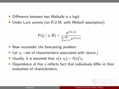
• Difference between two Weibulls is a logit
• Under Luce axioms (on R.U.M. with Weibull assumption)
Pr(j | s,B) =ev(s,xj )∑Nl=1 e
v(s,xl )
• Now reconsider the forecasting problem:
• Let xj =set of characteristics associated with choice j
• Usually, it is assumed that v(s, xj) = θ(s)′xj• Dependence of θon s reflects fact that individuals differ in their
evaluation of characteristics.
Heckman Classical Discrete Choice Theory
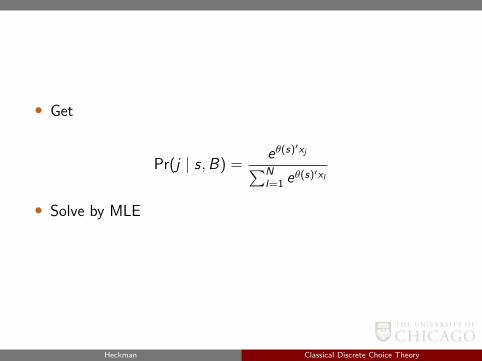
• Get
Pr(j | s,B) =eθ(s)′xj∑Nl=1 e
θ(s)′xl
• Solve by MLE
Heckman Classical Discrete Choice Theory
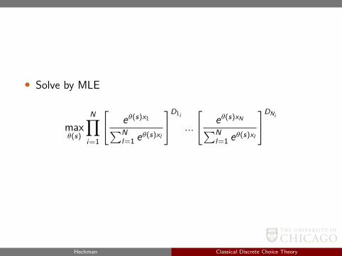
• Solve by MLE
maxθ(s)
N∏i=1
[eθ(s)x1∑Nl=1 e
θ(s)xl
]D1i
...
[eθ(s)xN∑Nl=1 e
θ(s)xl
]DNi
Heckman Classical Discrete Choice Theory
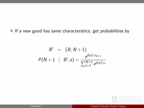
• If a new good has same characteristics, get probabilities by
B ′ = B ,N + 1
P(N + 1 | B ′, s) =eθ(s)′xN+1∑N+1l=1 eθ(s)′xl
Heckman Classical Discrete Choice Theory
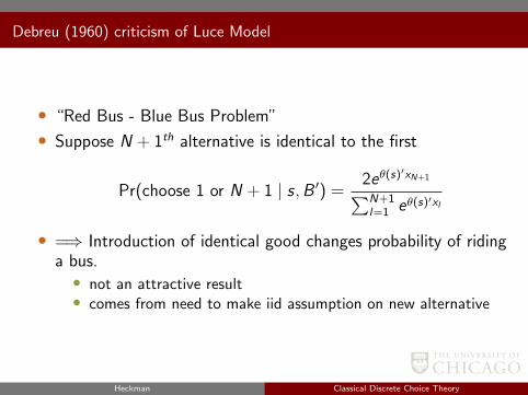
Debreu (1960) criticism of Luce Model
• “Red Bus - Blue Bus Problem”
• Suppose N + 1th alternative is identical to the first
Pr(choose 1 or N + 1 | s,B ′) =2eθ(s)′xN+1∑N+1l=1 eθ(s)′xl
• =⇒ Introduction of identical good changes probability of ridinga bus.• not an attractive result• comes from need to make iid assumption on new alternative
Heckman Classical Discrete Choice Theory
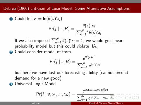
Debreu (1960) criticism of Luce Model: Some Alternative Assumptions
1 Could let vi = ln(θ(s)′xi)
Pr(j | s,B) =θ(s)′xj∑N+1l=1 θ(s)′xl
If we also imposed∑N
l=1 θ(s)′xl = 1, we would get linearprobability model but this could violate IIA.
2 Could consider model of form
Pr(j | s,B) =eθ
j (s)x i∑Nl=1 e
θl (s)xl
but here we have lost our forecasting ability (cannot predictdemand for a new good).
3 Universal Logit Model
Pr(i | s, x1, ..., xN) =eϕi (x1,...,xN)β(s)∑Nl=1 e
ϕl (x1,...,xN)β(s)
Here we lose IIA and forecasting (Bernstein PolynomialExpansion).
Heckman Classical Discrete Choice Theory

Criteria for a good PCS
1 Goal: We want a probabilistic choice model that
1 has a flexible functional form2 is computationally practical3 allows for flexibility in representing substitution patterns
among choices4 is consistent with a random utility model (RUM) =⇒ has a
structural interpretation
Heckman Classical Discrete Choice Theory
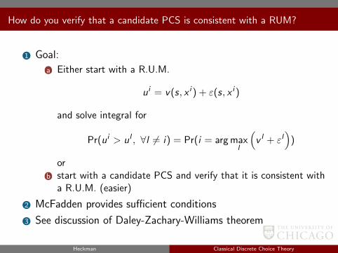
How do you verify that a candidate PCS is consistent with a RUM?
1 Goal:
(a) Either start with a R.U.M.
ui = v(s, x i ) + ε(s, x i )
and solve integral for
Pr(ui > ul , ∀l 6= i) = Pr(i = arg maxl
(v l + εl
))
or(b) start with a candidate PCS and verify that it is consistent with
a R.U.M. (easier)
2 McFadden provides sufficient conditions
3 See discussion of Daley-Zachary-Williams theorem
Heckman Classical Discrete Choice Theory

Link to Airum Models
Heckman Classical Discrete Choice Theory
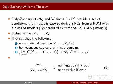
Daly-Zachary-Williams Theorem
• Daly-Zachary (1976) and Williams (1977) provide a set ofconditions that makes it easy to derive a PCS from a RUM witha class of models (“generalized extreme value” (GEV) models)
• Define G : G (Y1, . . . ,YJ)
• If G satisfies the following
1 nonnegative defined on Y1, . . . ,YJ ≥ 02 homogeneous degree one in its arguments3 lim
Yi→∞G (Y1, . . . ,Yi , . . . ,YJ)→∞, ∀i = 1, . . . , J
•
∂kG
∂Y1 · · · ∂Ykis
nonnegative if k oddnonpositive if even
(1)
Heckman Classical Discrete Choice Theory
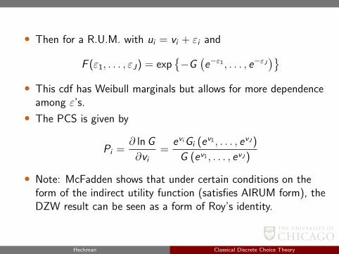
• Then for a R.U.M. with ui = vi + εi and
F (ε1, . . . , εJ) = exp−G
(e−ε1 , . . . , e−εJ
)• This cdf has Weibull marginals but allows for more dependence
among ε’s.
• The PCS is given by
Pi =∂ lnG
∂vi=
eviGi (ev1 , . . . , evJ )
G (ev1 , . . . , evJ )
• Note: McFadden shows that under certain conditions on theform of the indirect utility function (satisfies AIRUM form), theDZW result can be seen as a form of Roy’s identity.
Heckman Classical Discrete Choice Theory
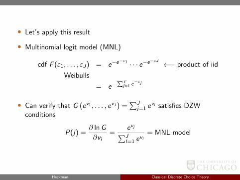
• Let’s apply this result
• Multinomial logit model (MNL)
cdf F (ε1, . . . , εJ) = e−e−ε1 · · · e−e−εJ ←− product of iid
Weibulls
= e−∑J
j=1 e−εj
• Can verify that G (ev1 , . . . , evJ ) =∑J
j=1 evi satisfies DZW
conditions
P(j) =∂ lnG
∂vi=
evj∑Jl=1 e
vl= MNL model
Heckman Classical Discrete Choice Theory
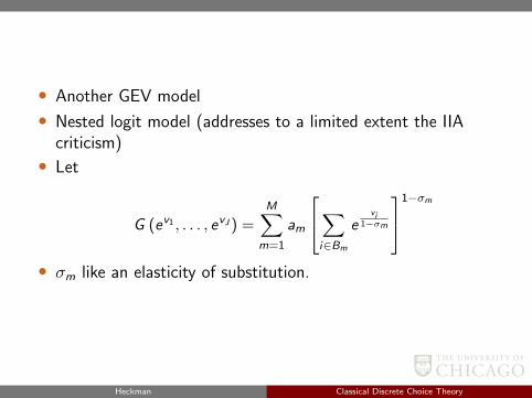
• Another GEV model
• Nested logit model (addresses to a limited extent the IIAcriticism)
• Let
G (ev1 , . . . , evJ ) =M∑
m=1
am
∑i∈Bm
evi
1−σm
1−σm
• σm like an elasticity of substitution.
Heckman Classical Discrete Choice Theory
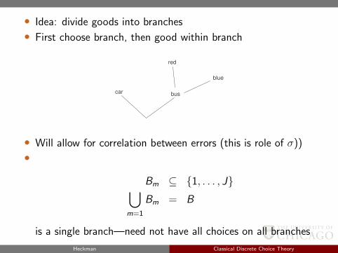
• Idea: divide goods into branches
• First choose branch, then good within branch
carbus
red
blue
• Will allow for correlation between errors (this is role of σ))
•
Bm ⊆ 1, . . . , J⋃m=1
Bm = B
is a single branch—need not have all choices on all branches
Heckman Classical Discrete Choice Theory
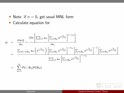
• Note: if σ = 0, get usual MNL form
• Calculate equation for
pi =∂ lnG
∂vi=
∂ ln
[∑mm=1 am
[∑i∈Bm
evi
1−σm
]1−σm]
∂vi
=
∑m3 i∈Bm
am
(e
vi1−σm
)[∑i∈Bm
evi
1−σm
]−σm [∑i∈Bm
evi
1−σm
]−1 [∑i∈Bm
evi
1−σm
]∑m
m=1 am
[∑i∈Bm
evi
1−σm
]1−σm
=m∑
m=1
P(i | Bm)P(Bm)
Heckman Classical Discrete Choice Theory
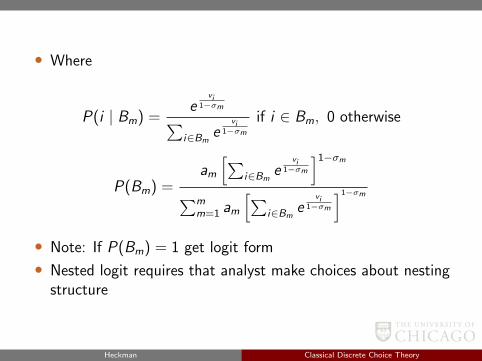
• Where
P(i | Bm) =e
vi1−σm∑
i∈Bme
vi1−σm
if i ∈ Bm, 0 otherwise
P(Bm) =am[∑
i∈Bme
vi1−σm
]1−σm
∑mm=1 am
[∑i∈Bm
evi
1−σm
]1−σm
• Note: If P(Bm) = 1 get logit form
• Nested logit requires that analyst make choices about nestingstructure
Heckman Classical Discrete Choice Theory
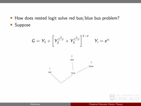
• How does nested logit solve red bus/blue bus problem?
• Suppose
G = Y1 +
[Y
11−σ
2 + Y1
1−σ3
]1−σ
Yi = evi
Heckman Classical Discrete Choice Theory
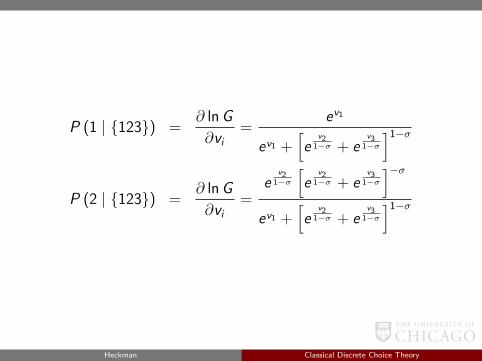
P (1 | 123) =∂ lnG
∂vi=
ev1
ev1 +[e
v21−σ + e
v31−σ
]1−σ
P (2 | 123) =∂ lnG
∂vi=
ev2
1−σ
[e
v21−σ + e
v31−σ
]−σev1 +
[e
v21−σ + e
v31−σ
]1−σ
Heckman Classical Discrete Choice Theory
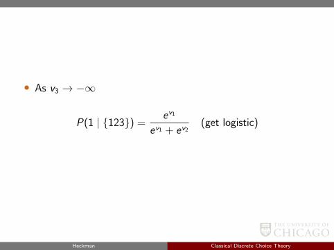
• As v3 → −∞
P(1 | 123) =ev1
ev1 + ev2(get logistic)
Heckman Classical Discrete Choice Theory
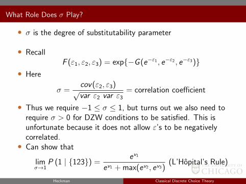
What Role Does σ Play?
• σ is the degree of substitutability parameter
• RecallF (ε1, ε2, ε3) = exp−G (e−ε1 , e−ε2 , e−ε3)
• Here
σ =cov(ε2, ε3)√var ε2 var ε3
= correlation coefficient
• Thus we require −1 ≤ σ ≤ 1, but turns out we also need torequire σ > 0 for DZW conditions to be satisfied. This isunfortunate because it does not allow ε’s to be negativelycorrelated.• Can show that
limσ→1
P (1 | 123) =ev1
ev1 + max(ev2 , ev3)(L’Hopital’s Rule)
Heckman Classical Discrete Choice Theory
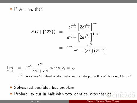
• If v2 = v3, then
P (2 | 123) =e
v21−σ
[2e
v21−σ
]−σev1 +
[2e
v21−σ
]1−σ
= 2−σev2
ev1 + (ev2) (21−σ)
limσ→1
= 2−1 ev2
ev1 + ev2when v1 = v2
introduce 3rd identical alternative and cut the probability of choosing 2 in half
• Solves red-bus/blue-bus problem
• Probability cut in half with two identical alternatives
Heckman Classical Discrete Choice Theory
car
red bus
blue bus
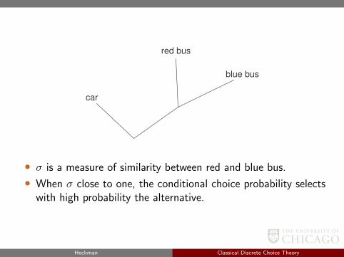
• σ is a measure of similarity between red and blue bus.
• When σ close to one, the conditional choice probability selectswith high probability the alternative.
Heckman Classical Discrete Choice Theory
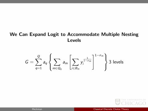
We Can Expand Logit to Accommodate Multiple NestingLevels
G =Q∑
q=1
aq
∑m∈Qq
am
[∑i∈Bm
y1
1−σmi
]1−σm 3 levels
Heckman Classical Discrete Choice Theory
• Example: Two Choices
1 Neighborhood (m)2 Transportation mode (t)3 P(m): choice of neighborhood4 P(i | Bm): probability of choosing i th mode, given
neighborhood m
Heckman Classical Discrete Choice Theory
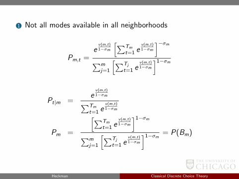
1 Not all modes available in all neighborhoods
Pm,t =e
v(m,t)1−σm
[∑Tm
t=1 ev(m,t)1−σm
]−σm∑m
j=1
[∑Tj
t=1 ev(m,t)1−σm
]1−σm
Pt|m =e
v(m,t)1−σm∑Tm
t=1 ev(m,t)1−σm
Pm =
[∑Tm
t=1 ev(m,t)1−σm
]1−σm
∑mj=1
[∑Tj
t=1 ev(m,t)1−σm
]1−σm = P(Bm)
Heckman Classical Discrete Choice Theory
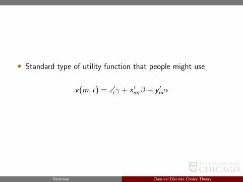
• Standard type of utility function that people might use
v(m, t) = z ′tγ + x ′mtβ + y ′mα
Heckman Classical Discrete Choice Theory
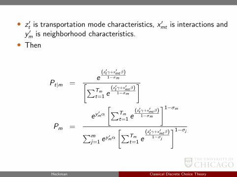
• z ′t is transportation mode characteristics, x ′mt is interactions andy ′m is neighborhood characteristics.
• Then
Pt|m =e
(z′tγ+x′mtβ)1−σm[∑Tm
t=1 e(z′tγ+x′mtβ)
1−σm
]
Pm =
ey′mα
[∑Tm
t=1 e(z′tγ+x′mtβ)
1−σm
]1−σm
∑mj=1 e
y ′mα
[∑Tm
t=1 e(z′tγ+x′mtβ)
1−σj
]1−σj
Heckman Classical Discrete Choice Theory
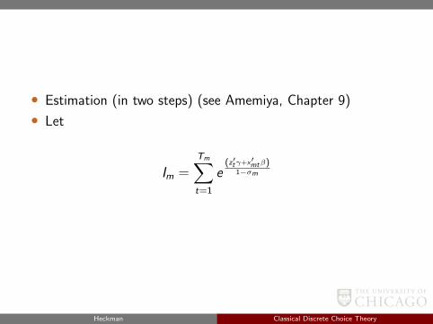
• Estimation (in two steps) (see Amemiya, Chapter 9)
• Let
Im =Tm∑t=1
e(z′tγ+x′mtβ)
1−σm
Heckman Classical Discrete Choice Theory
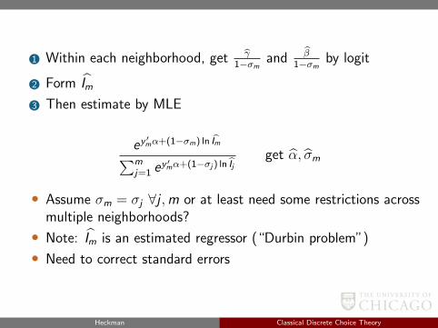
1 Within each neighborhood, get γ1−σm and β
1−σm by logit
2 Form Im
3 Then estimate by MLE
ey′mα+(1−σm) ln Im∑m
j=1 ey ′mα+(1−σj ) ln Ij
get α, σm
• Assume σm = σj ∀j ,m or at least need some restrictions acrossmultiple neighborhoods?
• Note: Im is an estimated regressor (“Durbin problem”)
• Need to correct standard errors
Heckman Classical Discrete Choice Theory
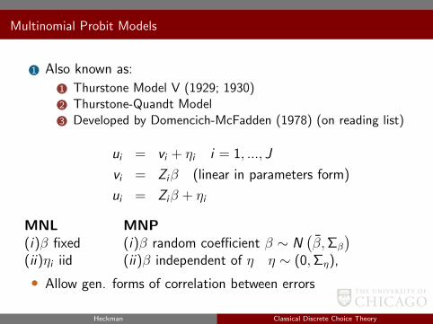
Multinomial Probit Models
1 Also known as:
1 Thurstone Model V (1929; 1930)2 Thurstone-Quandt Model3 Developed by Domencich-McFadden (1978) (on reading list)
ui = vi + ηi i = 1, ..., J
vi = Ziβ (linear in parameters form)
ui = Ziβ + ηi
MNL MNP(i)β fixed (i)β random coefficient β ∼ N
(β,Σβ
)(ii)ηi iid (ii)β independent of η η ∼ (0,Ση),
• Allow gen. forms of correlation between errors
Heckman Classical Discrete Choice Theory
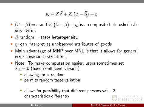
ui = Zi β + Zi
(β − β
)+ ηi
• (β − β) = ε and Zi
(β − β
)+ ηi is a composite heteroskedastic
error term.
• β random = taste heterogeneity,
• ηi can interpret as unobserved attributes of goods
• Main advantage of MNP over MNL is that it allows for generalerror covariance structure.
• Note: To make computation easier, users sometimes setΣβ = 0 (fixed coefficient version)• allowing for β random• permits random taste variation
• allows for possibility that different persons value 2characteristics differently
Heckman Classical Discrete Choice Theory
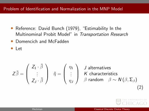
Problem of Identification and Normalization in the MNP Model
• Reference: David Bunch (1979), “Estimability In theMultinominal Probit Model” in Transportation Research
• Domencich and McFadden
• Let
Z β =
Z1 · β...
ZJ · β
η =
η1...ηJ
J alternativesK characteristicsβ random β ∼ N (β,Σβ)
(2)
Heckman Classical Discrete Choice Theory
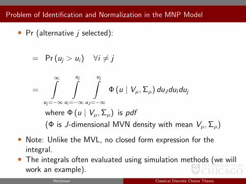
Problem of Identification and Normalization in the MNP Model
• Pr (alternative j selected):
= Pr (uj > ui) ∀i 6= j
=
∞∫uj=−∞
uj∫ui=−∞
uj∫uJ=−∞
Φ (u | Vµ,Σµ) duJdulduj
where Φ (u | Vµ,Σµ) is pdf
(Φ is J-dimensional MVN density with mean Vµ,Σµ)
• Note: Unlike the MVL, no closed form expression for theintegral.• The integrals often evaluated using simulation methods (we will
work an example).
Heckman Classical Discrete Choice Theory
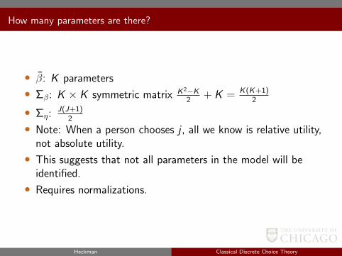
How many parameters are there?
• β: K parameters
• Σβ: K × K symmetric matrix K2−K2
+ K = K(K+1)2
• Ση: J(J+1)2
• Note: When a person chooses j , all we know is relative utility,not absolute utility.
• This suggests that not all parameters in the model will beidentified.
• Requires normalizations.
Heckman Classical Discrete Choice Theory
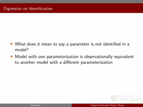
Digression on Identification
• What does it mean to say a parameter is not identified in amodel?
• Model with one parameterization is observationally equivalentto another model with a different parameterization
Heckman Classical Discrete Choice Theory
Digression on Identification
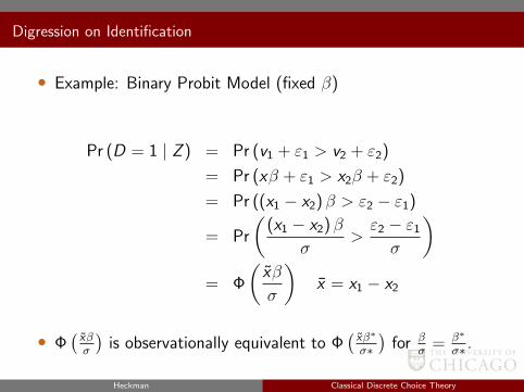
• Example: Binary Probit Model (fixed β)
Pr (D = 1 | Z ) = Pr (v1 + ε1 > v2 + ε2)
= Pr (xβ + ε1 > x2β + ε2)
= Pr ((x1 − x2) β > ε2 − ε1)
= Pr
((x1 − x2) β
σ>ε2 − ε1
σ
)= Φ
(xβ
σ
)x = x1 − x2
• Φ(xβσ
)is observationally equivalent to Φ
(xβ∗
σ∗
)for β
σ= β∗
σ∗ .
Heckman Classical Discrete Choice Theory
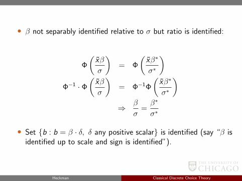
• β not separably identified relative to σ but ratio is identified:
Φ
(xβ
σ
)= Φ
(xβ∗
σ∗
)Φ−1 · Φ
(xβ
σ
)= Φ−1Φ
(xβ∗
σ∗
)⇒ β
σ=β∗
σ∗
• Set b : b = β · δ, δ any positive scalar is identified (say “β isidentified up to scale and sign is identified”).
Heckman Classical Discrete Choice Theory
Identification in the MVP model
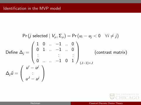
Pr (j selected | Vµ,Σµ) = Pr (ui − uj < 0 ∀i 6= j)
Define ∆j =
1 0 .. −1 .. 00 1 .. −1 .. 0: : :0 .. .. −1 0 1
(J−1)×J
(contrast matrix)
∆j u =
u′ − uj
:uJ − uj
Heckman Classical Discrete Choice Theory
Identification in the MVP model
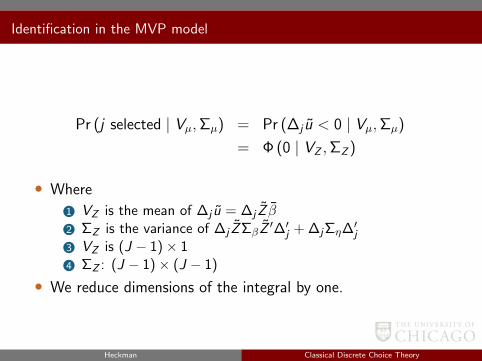
Pr (j selected | Vµ,Σµ) = Pr (∆j u < 0 | Vµ,Σµ)
= Φ (0 | VZ ,ΣZ )
• Where
1 VZ is the mean of ∆j u = ∆j Z β2 ΣZ is the variance of ∆j ZΣβZ
′∆′j + ∆jΣη∆′j3 VZ is (J − 1)× 14 ΣZ : (J − 1)× (J − 1)
• We reduce dimensions of the integral by one.
Heckman Classical Discrete Choice Theory
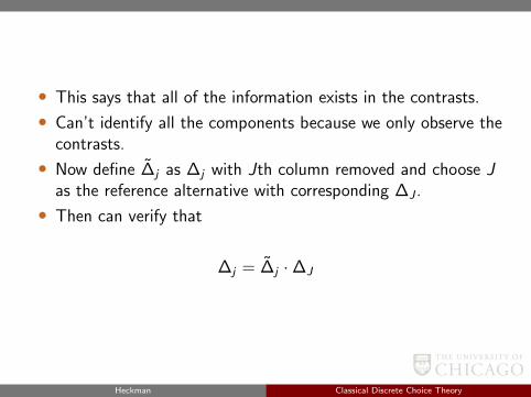
• This says that all of the information exists in the contrasts.
• Can’t identify all the components because we only observe thecontrasts.
• Now define ∆j as ∆j with Jth column removed and choose Jas the reference alternative with corresponding ∆J .
• Then can verify that
∆j = ∆j ·∆J
Heckman Classical Discrete Choice Theory
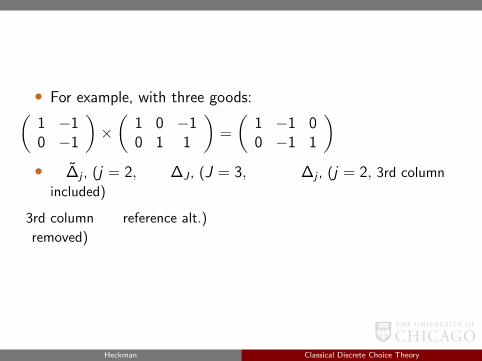
• For example, with three goods:(1 −10 −1
)×(
1 0 −10 1 1
)=
(1 −1 00 −1 1
)• ∆j , (j = 2, ∆J , (J = 3, ∆j , (j = 2, 3rd column
included)
3rd column
removed)
reference alt.)
Heckman Classical Discrete Choice Theory
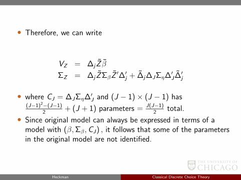
• Therefore, we can write
VZ = ∆j Z β
ΣZ = ∆j ZΣβZ′∆′j + ∆j∆JΣη∆′J∆′j
• where CJ = ∆JΣη∆′J and (J − 1)× (J − 1) has(J−1)2−(J−1)
2+ (J + 1) parameters = J(J−1)
2total.
• Since original model can always be expressed in terms of amodel with (β,Σβ,CJ) , it follows that some of the parametersin the original model are not identified.
Heckman Classical Discrete Choice Theory
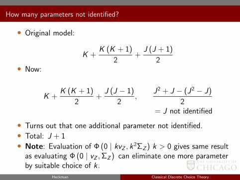
How many parameters not identified?
• Original model:
K +K (K + 1)
2+
J (J + 1)
2• Now:
K +K (K + 1)
2+
J (J − 1)
2,
J2 + J − (J2 − J)
2= J not identified
• Turns out that one additional parameter not identified.• Total: J + 1• Note: Evaluation of Φ (0 | kvZ , k2ΣZ ) k > 0 gives same result
as evaluating Φ (0 | vZ ,ΣZ ) can eliminate one more parameterby suitable choice of k .
Heckman Classical Discrete Choice Theory
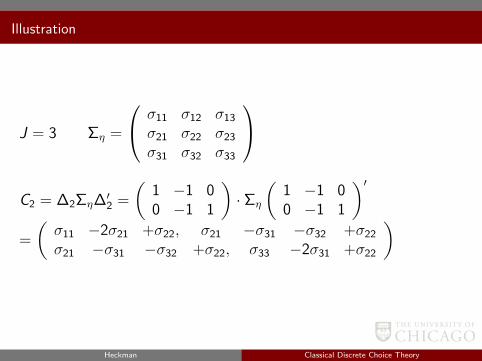
Illustration
J = 3 Ση =
σ11 σ12 σ13
σ21 σ22 σ23
σ31 σ32 σ33
C2 = ∆2Ση∆′2 =
(1 −1 00 −1 1
)· Ση
(1 −1 00 −1 1
)′=
(σ11 −2σ21 +σ22, σ21 −σ31 −σ32 +σ22
σ21 −σ31 −σ32 +σ22, σ33 −2σ31 +σ22
)
Heckman Classical Discrete Choice Theory
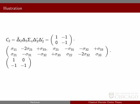
Illustration
C2 = ∆2∆3Ση∆′3∆′2 =
(1 −10 −1
)·(
σ11 −2σ21 +σ33, σ21 −σ31 −σ32 +σ33
σ21 −σ31 −σ32 +σ33 σ22 −2σ32 σ33
)·(
1 0−1 −1
)
Heckman Classical Discrete Choice Theory
Normalization Approach of Albreit, Lerman, and Manski (1978)
• Note: Need J + 1 restrictions on VCV matrix.
• Fix J parameters by setting last row and last column of Ση to 0
• Fix scale by constraining diagonal elements of Ση so that traceΣεJ
equals variance of a standard Weibull. (To compareestimates with MNL and independent probit)
Heckman Classical Discrete Choice Theory
How do we solve the forecasting problem?
• Suppose that we have 2 goods and add a 3rd
Pr (1 chosen) = Pr(u1 − u2 ≥ 0
)= Pr 1
((Z 1 − Z 2
)β ≥ ω2 − ω1
)• Define η1, η2, η3 as random choice specific shocks independent
of Z 1,Z 2 and Z 3.
• (β − β) arises from variability in slop coefficients.
Heckman Classical Discrete Choice Theory

• Define:
ω1 = Z 1(β − β
)+ η1, ω2 = Z 2
(β − β
)+ η2
=
∫ (Z1−Z2)β
[σ11+σ22−2σ12+(Z2−Z1)Σβ(Z2−Z1)′]1/2
−∞
1√2π
e−t/2dt
• Pr(1 chosen).
• Now add a 3rd good
u3 = Z 3β + Z 3(β − β
)+ η3.
Heckman Classical Discrete Choice Theory
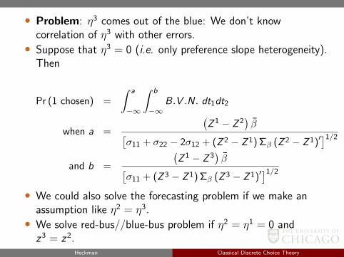
• Problem: η3 comes out of the blue: We don’t knowcorrelation of η3 with other errors.• Suppose that η3 = 0 (i.e. only preference slope heterogeneity).
Then
Pr (1 chosen) =
∫ a
−∞
∫ b
−∞B.V .N. dt1dt2
when a =
(Z 1 − Z 2
)β[
σ11 + σ22 − 2σ12 + (Z 2 − Z 1) Σβ (Z 2 − Z 1)′]1/2
and b =
(Z 1 − Z 3
)β[
σ11 + (Z 3 − Z 1) Σβ (Z 3 − Z 1)′]1/2
• We could also solve the forecasting problem if we make anassumption like η2 = η3.• We solve red-bus//blue-bus problem if η2 = η1 = 0 andz3 = z2.
Heckman Classical Discrete Choice Theory
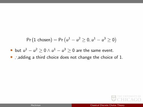
Pr (1 chosen) = Pr(u1 − u2 ≥ 0, u1 − u3 ≥ 0
)• but u1 − u2 ≥ 0 ∧ u1 − u3 ≥ 0 are the same event.
• ∴adding a third choice does not change the choice of 1.
Heckman Classical Discrete Choice Theory
Estimation Methods for MNP Models
• Models tend to be difficult to estimate because of highdimensional integrals.
• Integrals need to be evaluated at each stage of estimating thelikelihood.
• Simulation provides a means of estimating Pij = Pr (ichooses j)
Heckman Classical Discrete Choice Theory

Computation and Estimation
Link to Appendix
Heckman Classical Discrete Choice Theory
Classical Models for Estimating Models with Limited Dependent Variables
References:
• Amemiya, Ch. 10
• Different types of sampling (previously discussed)
(a) random sampling(b) censored sampling(c) truncated sampling(d) other non-random (exogenous stratified, choice-based)
Heckman Classical Discrete Choice Theory

Standard Tobit Model (Tobin, 1958) “Type I Tobit”
y ∗i = xiβ + ui
• Observe, i.e.,
yi = y ∗i if y ∗i ≥ y0 or yi = 1 (y ∗i ≥ y0) y ∗iyi = 0 if y ∗i < y0
yi = 1 (y ∗i < y0)y ∗i
• Tobin’s example-expenditure on a durable good only observed ifgood is purchased
Heckman Classical Discrete Choice Theory
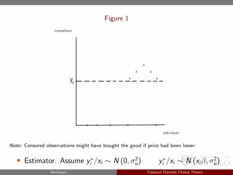
Figure 1
individuals
y0
x
x
x
x
x
x x x x x
expenditure
Note: Censored observations might have bought the good if price had been lower.
• Estimator. Assume y ∗i /xi ∼ N (0, σ2u) y ∗i /xi ∼ N (xiβ, σ
2u)
Heckman Classical Discrete Choice Theory
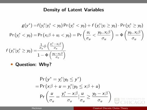
Density of Latent Variables
g(y∗) =f (y∗i |y∗i < y0) Pr (y∗i < y0) + f (y∗i |yi ≥ y0) · Pr (y∗i ≥ y0)
Pr (y∗i < y0) = Pr (xiβ + ui < y0) = Pr
(uiσu
<y0−xiβ
σu
)= Φ
(y0−xiβ
σu
)
f (y∗i |y∗i ≥ y0) =
1σuφ(y∗i −xiβσu
)1− Φ
(y0−xiβσu
)• Question: Why?
Pr (y ∗ = y ∗i |y0 ≤ y ∗)
= Pr (xβ + u = y ∗i |y0 ≤ xβ + u)
Pr
(u
σu=
y ∗i − xβ
σu| uσu≥ y0 − xβ
σu
)Heckman Classical Discrete Choice Theory
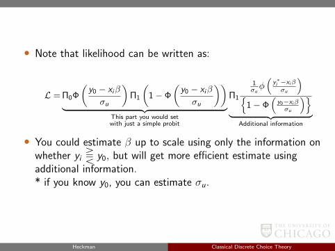
• Note that likelihood can be written as:
L = Π0Φ
(y0 − xiβ
σu
)Π1
(1− Φ
(y0 − xiβ
σu
))︸ ︷︷ ︸
This part you would setwith just a simple probit
Π1
1σuφ(
y∗i −xiβσu
)
1− Φ(
y0−xiβσu
)︸ ︷︷ ︸
Additional information
• You could estimate β up to scale using only the information onwhether yi T y0, but will get more efficient estimate usingadditional information.* if you know y0, you can estimate σu.
Heckman Classical Discrete Choice Theory

Truncated Version of Type I Tobit
Observe yi = y ∗i if y ∗i > o(observe nothing for truncated observationsexample: only observe wages for workers
)
Likelihood: L = Π1
1σuφ(
y∗i −xiβσu
)Φ(
xiβσu
)Pr (y ∗i > 0) = Pr (xβ + u > 0)
= Pr
(u
σu>−xβσu
)= Pr
(u <
xβ
σu
)
Heckman Classical Discrete Choice Theory
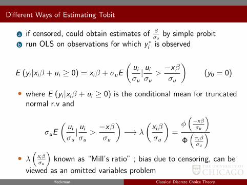
Different Ways of Estimating Tobit
(a) if censored, could obtain estimates of βσu
by simple probit
(b) run OLS on observations for which y ∗i is observed
E (yi |xiβ + ui ≥ 0) = xiβ + σuE
(uiσu| uiσu
>−xβσu
)(y0 = 0)
• where E (yi |xiβ + ui ≥ 0) is the conditional mean for truncatednormal r.v and
σuE
(uiσu| uiσu
>−xβσu
)−→ λ
(xiβ
σu
)=φ(−xβσu
)Φ(πiβσu
)• λ
(xiβσu
)known as “Mill’s ratio” ; bias due to censoring, can be
viewed as an omitted variables problemHeckman Classical Discrete Choice Theory
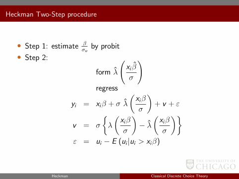
Heckman Two-Step procedure
• Step 1: estimate βσu
by probit
• Step 2:
form λ
(xi β
σ
)regress
yi = xiβ + σ λ
(xiβ
σ
)+ v + ε
v = σ
λ
(xiβ
σ
)− λ
(xiβ
σ
)ε = ui − E (ui |ui > xiβ)
Heckman Classical Discrete Choice Theory
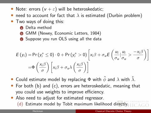
• Note: errors (v + ε) will be heteroskedatic;• need to account for fact that λ is estimated (Durbin problem)• Two ways of doing this:
(a) Delta method(b) GMM (Newey, Economic Letters, 1984)(c) Suppose you run OLS using all the data
E (yi ) = Pr (y∗i ≤ 0) · 0 + Pr (y∗i > 0)
[xiβ + σuE
(uiσu| uiσu
>−xiβσ
)]=Φ
(xiβ
σ
)[xiβ + σuλ
(xiβ
σ
)]• Could estimate model by replacing Φ with φ and λ with λ.• For both (b) and (c), errors are heteroskedatic, meaning that
you could use weights to improve efficiency.• Also need to adjust for estimated regressor.
(d) Estimate model by Tobit maximum likelihood directly.
Heckman Classical Discrete Choice Theory
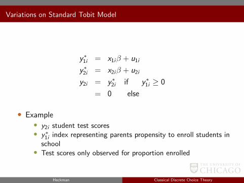
Variations on Standard Tobit Model
y ∗1i = x1iβ + u1i
y ∗2i = x2iβ + u2i
y2i = y ∗2i if y ∗1i ≥ 0
= 0 else
• Example• y2i student test scores• y∗1i index representing parents propensity to enroll students in
school• Test scores only observed for proportion enrolled
Heckman Classical Discrete Choice Theory
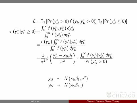
L =Π1 [Pr (y ∗1i > 0) f (y2i |y ∗1i > 0)] Π0 [Pr (y ∗1i ≤ 0)]
f (y ∗2i |y ∗1i ≥ 0) =
∫∞0
f (y ∗1i , y∗2i) dy
∗1i∫∞
0f (y ∗1i) dy
∗1i
=f (y2i)
∫∞0
f (y ∗1i |y ∗2i) dy ∗1i∫∞0
f (y ∗1i) dy∗1i
=1
σ2φ
(y ∗2i − x2iβ2
σ2
)·∫∞
0f (y ∗1i |y ∗2i) dy ∗1i
Pr (y ∗1i > 0)
y1i ∼ N(x1iβ1, σ
2)
y2i ∼ N (x2iβ2, )
Heckman Classical Discrete Choice Theory
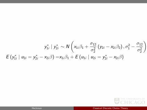
y ∗1i | y ∗2i ∼ N
(x1iβ1 +
σ12
σ22
(y2i − x2iβ2) , σ21 −
σ12
σ22
)E (y ∗1i | u2i = y ∗2i − x2iβ) =x1iβ1 + E (u1i | u2i = y ∗2i − x2iβ)
Heckman Classical Discrete Choice Theory
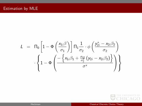
Estimation by MLE
L = Π0
[1− Φ
(x1iβ
σ1
)]Π1
1
σ2· φ(y ∗2i − x2iβ2
σ2
)
·
1− Φ
−x1iβ1 + σ12
σ22
(y2i − x2iβ2)
σx
Heckman Classical Discrete Choice Theory
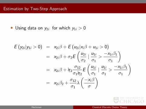
Estimation by Two-Step Approach
• Using data on y2i for which y1i > 0
E (y2i |y1i > 0) = x2iβ + E (u2i |xiβ + u1i > 0)
= x2iβ + σ2E
(u2i
σ2| u1i
σ1>−x1iβ1
σ1
)= x2iβ + \σ2
σ12
σ1\σ2E
(u1i
σ1| u1i
σ1>−x1iβ1
σ1
)= x2iβ2 +
σ12
σ1λ
(−xiβσ
)
Heckman Classical Discrete Choice Theory
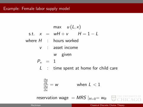
Example: Female labor supply model
max u (L, x)
s.t. x = wH + v H = 1− L
where H : hours worked
v : asset income
w given
Px = 1
L : time spent at home for child care
∂u∂L∂u∂x
= w when L < 1
reservation wage = MRS |H=0= wR
Heckman Classical Discrete Choice Theory
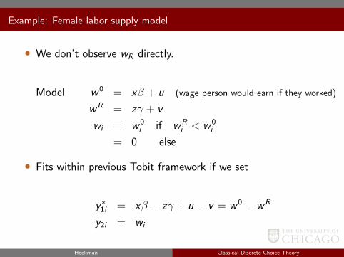
Example: Female labor supply model
• We don’t observe wR directly.
Model w 0 = xβ + u (wage person would earn if they worked)
wR = zγ + v
wi = w 0i if wR
i < w 0i
= 0 else
• Fits within previous Tobit framework if we set
y ∗1i = xβ − zγ + u − v = w 0 − wR
y2i = wi
Heckman Classical Discrete Choice Theory
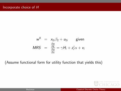
Incorporate choice of H
w 0 = x2iβ2 + u2i given
MRS =∂u∂L∂u∂x
= γHi + z ′iα + vi
(Assume functional form for utility function that yields this)
Heckman Classical Discrete Choice Theory
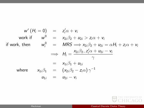
w r (Hi = 0) = z ′iα + vi
work if w 0 = x2iβ2 + u2i > ziα + vi
if work, then w 0i = MRS =⇒ x2iβ2 + u2i = αHi + ziα + vi
=⇒ Hi =x2iβ2−z
′iα + u2i − viγ
= x1iβ1 + u1i
where x1iβ1 = (x2iβ2 − ziα) γ−1
u1i = u2i − vi
Heckman Classical Discrete Choice Theory
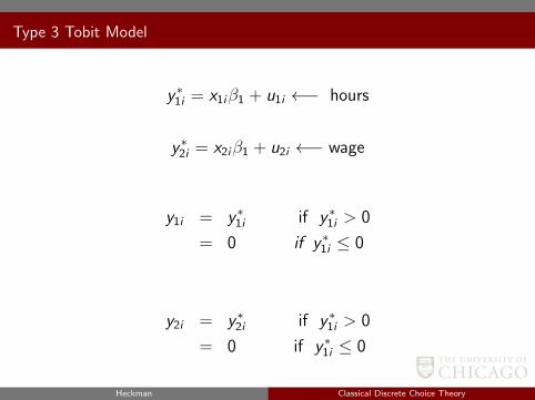
Type 3 Tobit Model
y ∗1i = x1iβ1 + u1i ←− hours
y ∗2i = x2iβ1 + u2i ←− wage
y1i = y ∗1i if y ∗1i > 0
= 0 if y ∗1i ≤ 0
y2i = y ∗2i if y ∗1i > 0
= 0 if y ∗1i ≤ 0
Heckman Classical Discrete Choice Theory
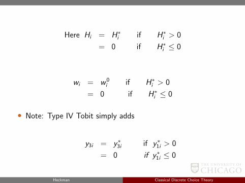
Here Hi = H∗i if H∗i > 0
= 0 if H∗i ≤ 0
wi = w 0i if H∗i > 0
= 0 if H∗i ≤ 0
• Note: Type IV Tobit simply adds
y3i = y ∗3i if y ∗1i > 0
= 0 if y ∗1i ≤ 0
Heckman Classical Discrete Choice Theory

• Can estimate by
(1) maximum likelihood(2) Two-step method
E(w 0i | Hi > 0
)= γHi + ziα + E (vi | Hi > 0)
Heckman Classical Discrete Choice Theory
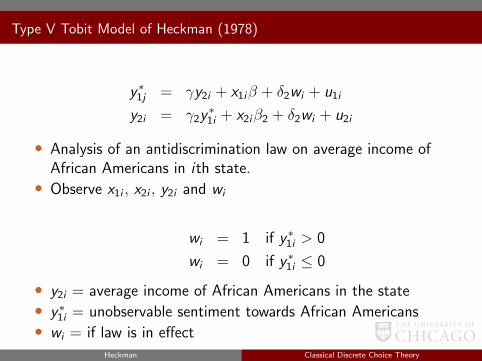
Type V Tobit Model of Heckman (1978)
y ∗1j = γy2i + x1iβ + δ2wi + u1i
y2i = γ2y∗1i + x2iβ2 + δ2wi + u2i
• Analysis of an antidiscrimination law on average income ofAfrican Americans in ith state.• Observe x1i , x2i , y2i and wi
wi = 1 if y ∗1i > 0
wi = 0 if y ∗1i ≤ 0
• y2i = average income of African Americans in the state• y ∗1i = unobservable sentiment towards African Americans• wi = if law is in effect
Heckman Classical Discrete Choice Theory
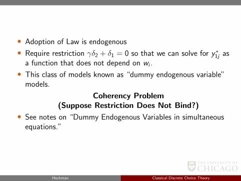
• Adoption of Law is endogenous
• Require restriction γδ2 + δ1 = 0 so that we can solve for y ∗1j asa function that does not depend on wi .
• This class of models known as “dummy endogenous variable”models.
Coherency Problem(Suppose Restriction Does Not Bind?)
• See notes on “Dummy Endogenous Variables in simultaneousequations.”
Heckman Classical Discrete Choice Theory
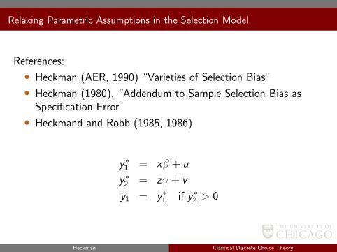
Relaxing Parametric Assumptions in the Selection Model
References:
• Heckman (AER, 1990) “Varieties of Selection Bias”
• Heckman (1980), “Addendum to Sample Selection Bias asSpecification Error”
• Heckmand and Robb (1985, 1986)
y ∗1 = xβ + u
y ∗2 = zγ + v
y1 = y ∗1 if y ∗2 > 0
Heckman Classical Discrete Choice Theory
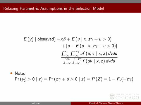
Relaxing Parametric Assumptions in the Selection Model
E (y ∗1 | observed) =xβ + E (u | x , zγ + u > 0)
+ [u − E (u | x , zγ + u > 0)]∫∞−∞
∫ −zγ−∞ uf (u, v | x , z) dvdu∫∞
−∞
∫ −zγ−∞ f (uv | x , z) dvdu
• Note:Pr (y ∗2 > 0 | z) = Pr (zγ + u > 0 | z) = P (Z ) = 1− Fv (−zγ)
Heckman Classical Discrete Choice Theory
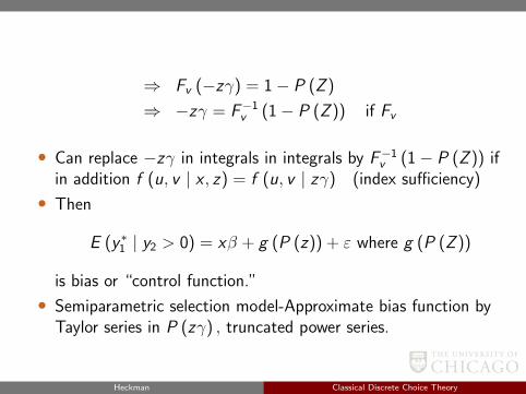
⇒ Fv (−zγ) = 1− P (Z )
⇒ −zγ = F−1v (1− P (Z )) if Fv
• Can replace −zγ in integrals in integrals by F−1v (1− P (Z )) if
in addition f (u, v | x , z) = f (u, v | zγ) (index sufficiency)
• Then
E (y ∗1 | y2 > 0) = xβ + g (P (z)) + ε where g (P (Z ))
is bias or “control function.”
• Semiparametric selection model-Approximate bias function byTaylor series in P (zγ) , truncated power series.
Heckman Classical Discrete Choice Theory

Airum Models
Heckman Classical Discrete Choice Theory
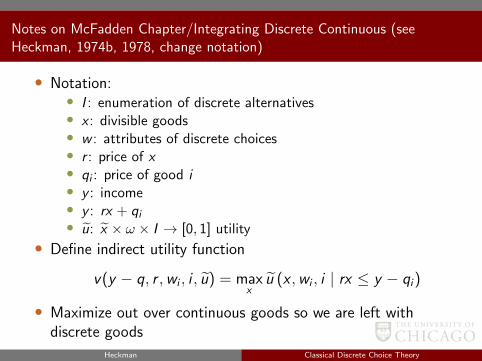
Notes on McFadden Chapter/Integrating Discrete Continuous (seeHeckman, 1974b, 1978, change notation)
• Notation:• I : enumeration of discrete alternatives• x : divisible goods• w : attributes of discrete choices• r : price of x• qi : price of good i• y : income• y : rx + qi• u: x × ω × I → [0, 1] utility
• Define indirect utility function
v(y − q, r ,wi , i , u) = maxx
u (x ,wi , i | rx ≤ y − qi)
• Maximize out over continuous goods so we are left withdiscrete goods
Heckman Classical Discrete Choice Theory
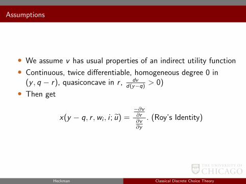
Assumptions
• We assume v has usual properties of an indirect utility function
• Continuous, twice differentiable, homogeneous degree 0 in(y , q − r), quasiconcave in r , dv
d(y−q)> 0)
• Then get
x(y − q, r ,wi , i ; u) =−∂v∂r∂v∂y
. (Roy’s Identity)
Heckman Classical Discrete Choice Theory
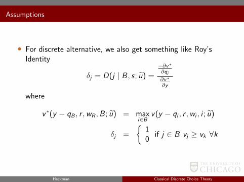
Assumptions
• For discrete alternative, we also get something like Roy’sIdentity
δj = D(j | B , s; u) =
−∂v∗∂qj∂v∗
∂y
where
v ∗(y − qB , r ,wR ,B ; u) = maxi∈B
v(y − qi , r ,wi , i ; u)
δj =
10
if j ∈ B vj ≥ vk ∀k
Heckman Classical Discrete Choice Theory
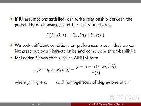
• If IU assumptions satisfied, can write relationship between theprobability of choosing ji and the utility function as
P(j | B , s) = Eu|sD(j | B , s; u)
• We seek sufficient conditions on preferences u such that we canintegrate out over characteristics and come up with probabilities
• McFadden Shows that v takes AIRUM form
v(y − q, r ,wi , i ; u) =y − q − α(r ,wi , i , u)
β(r)
where y > q + α α, β homogeneous of degree one wrt r
Heckman Classical Discrete Choice Theory
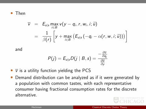
• Then
v = Eu|s maxi∈B
v(y − qi , r ,wi , i ; u)
=1
β(r)
[y + max
i∈B
(Eu|s (−qi − α(r ,w , i ; u))
)]and
P(j) = Eu|sD(j | B , s) =− ∂v∂qj∂v∂y
• v is a utility function yielding the PCS
• Demand distribution can be analyzed as if it were generated bya population with common tastes, with each representativeconsumer having fractional consumption rates for the discretealternative.
Heckman Classical Discrete Choice Theory
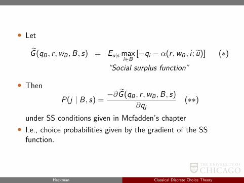
• Let
G (qB , r ,wB ,B , s) = Eu|s maxi∈B
[−qi − α(r ,wB , i ; u)] (∗)
“Social surplus function”
• Then
P(j | B , s) =−∂G (qB , r ,wB ,B , s)
∂qj(∗∗)
under SS conditions given in Mcfadden’s chapter
• I.e., choice probabilities given by the gradient of the SSfunction.
Heckman Classical Discrete Choice Theory

Return to main text
Heckman Classical Discrete Choice Theory

Appendix
Heckman Classical Discrete Choice Theory
Variety of Simulation Methods
• Simulated method of moments• Method of simulated scores• Simulated maximum likelihood
References:
• Lerman and Manski (1981), Structural Analysis (online atMcFadden’s website)• McFadden (1989), Econometrica• Ruud (1982), Journal of Econometrics• Hajivassilon and McFadden (1990)• Hajivassilon and Ruud (Ch. 20), Handbook of Econometrics• Stern (1992), Econometrica• Stern (1997), Survey in JEL• Bayesian MCMC (Chib et al. on reading list)
Heckman Classical Discrete Choice Theory
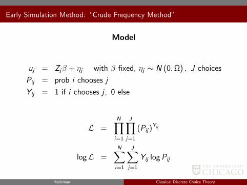
Early Simulation Method: “Crude Frequency Method”
Model
uj = Zjβ + ηj with β fixed, ηj ∼ N (0,Ω) , J choices
Pij = prob i chooses j
Yij = 1 if i chooses j , 0 else
L =N∏i=1
J∏j=1
(Pij)Yij
logL =N∑i=1
J∑j=1
Yij logPij
Heckman Classical Discrete Choice Theory
Simulation Algorithm
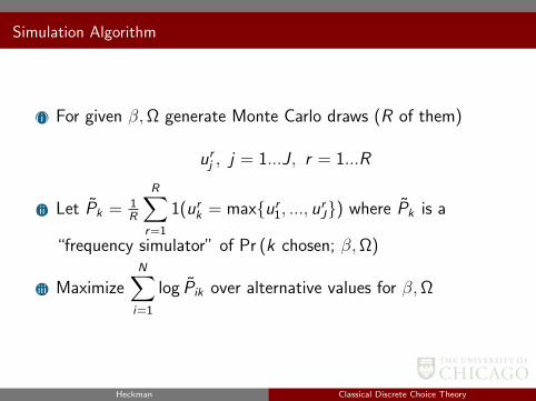
(i) For given β,Ω generate Monte Carlo draws (R of them)
urj , j = 1...J , r = 1...R
(ii) Let Pk = 1R
R∑r=1
1(urk = maxur
1, ..., urJ) where Pk is a
“frequency simulator” of Pr (k chosen; β,Ω)
(iii) MaximizeN∑i=1
log Pik over alternative values for β,Ω
Heckman Classical Discrete Choice Theory
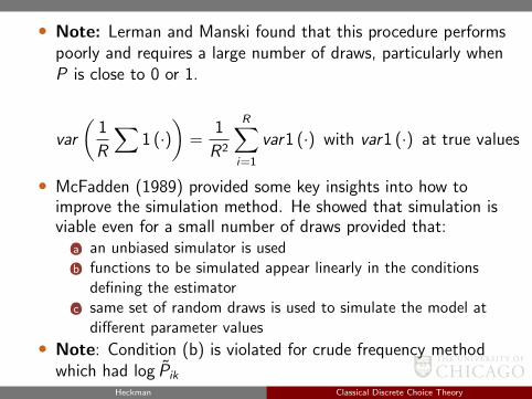
• Note: Lerman and Manski found that this procedure performspoorly and requires a large number of draws, particularly whenP is close to 0 or 1.
var
(1
R
∑1 (·)
)=
1
R2
R∑i=1
var1 (·) with var1 (·) at true values
• McFadden (1989) provided some key insights into how toimprove the simulation method. He showed that simulation isviable even for a small number of draws provided that:
(a) an unbiased simulator is used(b) functions to be simulated appear linearly in the conditions
defining the estimator(c) same set of random draws is used to simulate the model at
different parameter values
• Note: Condition (b) is violated for crude frequency methodwhich had log Pik
Heckman Classical Discrete Choice Theory
Simulated Method of Moments (McFadden, Econometrica, 1989)
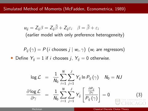
uij = Zijβ = Zij β + Zijεi β = β + εi
(earlier model with only preference heterogeneity)
Pij (γ) = P (i chooses j | wi , γ) (wi are regressors)
• Define Yij = 1 if i chooses j , Yij = 0 otherwise.
logL =1
N0
N∑i=1
J∑j=1
Yij lnPij (γ) N0 = NJ
∂ logL∂γ
=1
N0
N∑i=1
J∑j=1
Yij
[ ∂Pij
∂γ
Pij (γ)
]= 0 (3)
Heckman Classical Discrete Choice Theory
Simulated Method of Moments (McFadden, Econometrica, 1989)
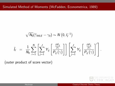
√N0(γMLE − γ0) ∼ N
(0, I−1
f
)If =
1
N0
N∑i=1
[J∑
j=1
Yij
[ ∂Pij
∂γ
Pij (γ)
]] J∑j=1
Yij
[ ∂Pij
∂γ
Pij (γ)
]′ .(outer product of score vector)
Heckman Classical Discrete Choice Theory
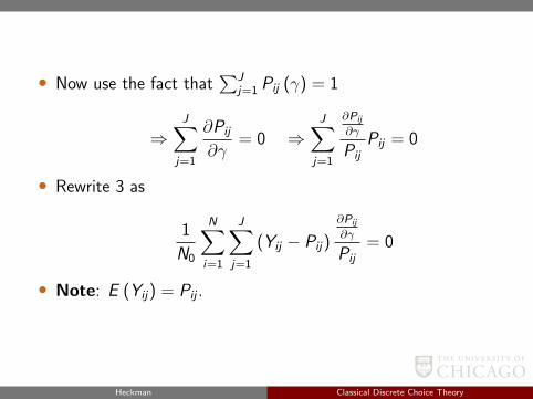
• Now use the fact that∑J
j=1 Pij (γ) = 1
⇒J∑
j=1
∂Pij
∂γ= 0 ⇒
J∑j=1
∂Pij
∂γ
PijPij = 0
• Rewrite 3 as
1
N0
N∑i=1
J∑j=1
(Yij − Pij)
∂Pij
∂γ
Pij= 0
• Note: E (Yij) = Pij .
Heckman Classical Discrete Choice Theory
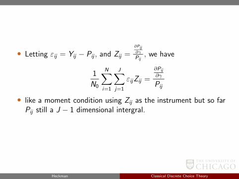
• Letting εij = Yij − Pij , and Zij =∂Pij∂γ
Pij, we have
1
N0
N∑i=1
J∑j=1
εijZij =
∂Pij
∂γ
Pij
• like a moment condition using Zij as the instrument but so farPij still a J − 1 dimensional intergral.
Heckman Classical Discrete Choice Theory
Simulation Algorithm
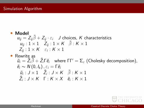
• Modeluij = Zij β + Zij · εi J choices, K characteristicsuij : 1× 1 Zij : 1× K β : K × 1Zij : 1× K εi : K × 1
• Rewrite asui = Zi β + ZiΓei where ΓΓ′ = Σε (Cholesky decomposition),ei ∼ N (0, Ik) , εi = Γeiui : J × 1 Zi : J × K β : K × 1
Zi : J × K Γ : K × X ei : K × 1
Heckman Classical Discrete Choice Theory
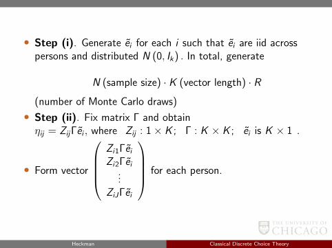
• Step (i). Generate ei for each i such that ei are iid acrosspersons and distributed N (0, Ik) . In total, generate
N (sample size) · K (vector length) · R
(number of Monte Carlo draws)
• Step (ii). Fix matrix Γ and obtainηij = ZijΓei , where Zij : 1× K ; Γ : K × K ; ei is K × 1 .
• Form vector
Zi1ΓeiZi2Γei
...ZiJΓei
for each person.
Heckman Classical Discrete Choice Theory
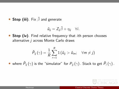
• Step (iii). Fix β and generate
uij = Zij β + ηij ∀i .• Step (iv). Find relative frequency that ith person chooses
alternative j across Monte Carlo draws
Pij (γ) =1
R
R∑r=1
1 (uij > uim; ∀m 6= j)
• where Pij (γ) is the “simulator” for Pij (γ) . Stack to get Pi (γ) .
Heckman Classical Discrete Choice Theory
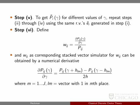
• Step (v). To get Pi (γ) for different values of γ, repeat steps(ii) through (iv) using the same r.v.’s ei generated in step (i).
• Step (vi). Define
wij =
∂Pij (γ)
∂γ
Pij
• and wij as corresponding stacked vector simulator for wij can beobtained by a numerical derivative
∂Pij (γ)
∂γ=
Pij (γ + hlm)− Pij (γ − hlm)
2h
where m = 1...J , lm = vector with 1 in mth place.
Heckman Classical Discrete Choice Theory
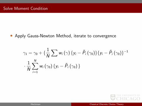
Solve Moment Condition
• Apply Gauss-Newton Method, iterate to convergence
γ1 = γ0 + 1
N
∑wi (γ) yi − Pi (γ0)yi − Pi (γ0)−1
· 1
N
N∑i=1
wi (γ0) yi − Pi (γ0)
Heckman Classical Discrete Choice Theory
Solve Moment Condition
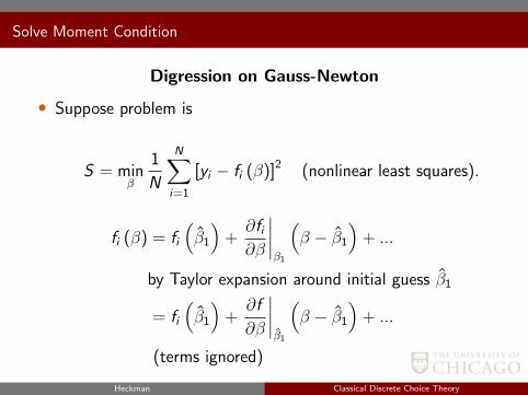
Digression on Gauss-Newton
• Suppose problem is
S = minβ
1
N
N∑i=1
[yi − fi (β)]2 (nonlinear least squares).
fi (β) = fi(β1
)+∂fi∂β
∣∣∣∣β1
(β − β1
)+ ...
by Taylor expansion around initial guess β1
= fi(β1
)+∂f
∂β
∣∣∣∣β1
(β − β1
)+ ...
(terms ignored)
Heckman Classical Discrete Choice Theory
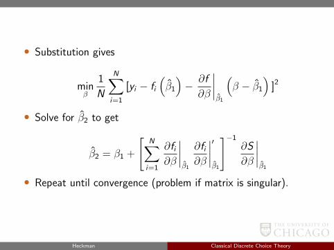
• Substitution gives
minβ
1
N
N∑i=1
[yi − fi(β1
)− ∂f
∂β
∣∣∣∣β1
(β − β1
)]2
• Solve for β2 to get
β2 = β1 +
[N∑i=1
∂fi∂β
∣∣∣∣β1
∂fi∂β
∣∣∣∣′β1
]−1
∂S
∂β
∣∣∣∣β1
• Repeat until convergence (problem if matrix is singular).
Heckman Classical Discrete Choice Theory
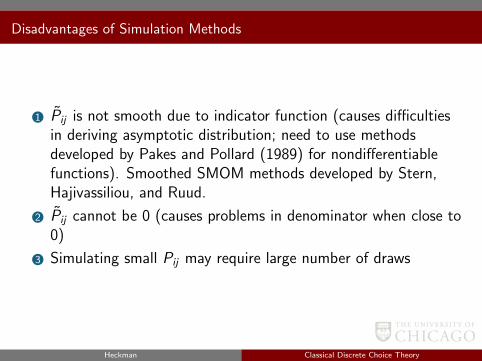
Disadvantages of Simulation Methods
1 Pij is not smooth due to indicator function (causes difficultiesin deriving asymptotic distribution; need to use methodsdeveloped by Pakes and Pollard (1989) for nondifferentiablefunctions). Smoothed SMOM methods developed by Stern,Hajivassiliou, and Ruud.
2 Pij cannot be 0 (causes problems in denominator when close to0)
3 Simulating small Pij may require large number of draws
Heckman Classical Discrete Choice Theory
Disadvantages of Simulation Methods
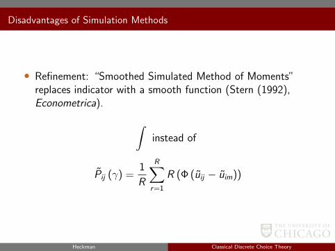
• Refinement: “Smoothed Simulated Method of Moments”replaces indicator with a smooth function (Stern (1992),Econometrica). ∫
instead of
Pij (γ) =1
R
R∑r=1
R (Φ (uij − uim))
Heckman Classical Discrete Choice Theory
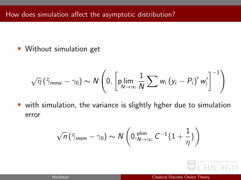
How does simulation affect the asymptotic distribution?
• Without simulation get
√η (γmme − γ0) ∼ N
(0,
[p limN→∞
1
N
∑wi (yi − Pi)
′ w ′i
]−1)
• with simulation, the variance is slightly hgher due to simulationerror
√n (γmsm − γ0) ∼ N
(0,plim
N→∞ C−11 +1
η)
Heckman Classical Discrete Choice Theory
How does simulation affect the asymptotic distribution?
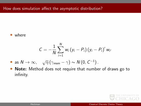
• where
C = − 1
N
N∑i=1
wi (yi − Pi) (yi − Pi)′ wi ′
• as N →∞, √η (γmsm − γ) ∼ N (0,C−1) .
• Note: Method does not require that number of draws go toinfinity.
Heckman Classical Discrete Choice Theory
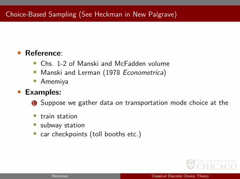
Choice-Based Sampling (See Heckman in New Palgrave)
• Reference:• Chs. 1-2 of Manski and McFadden volume• Manski and Lerman (1978 Econometrica)• Amemiya
• Examples:
1. Suppose we gather data on transportation mode choice at the
• train station• subway station• car checkpoints (toll booths etc.)
Heckman Classical Discrete Choice Theory
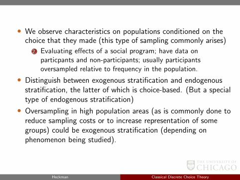
• We observe characteristics on populations conditioned on thechoice that they made (this type of sampling commonly arises)
2. Evaluating effects of a social program; have data onparticpants and non-participants; usually participantsoversampled relative to frequency in the population.
• Distinguish between exogenous stratification and endogenousstratification, the latter of which is choice-based. (But a specialtype of endogenous stratification)
• Oversampling in high population areas (as is commonly done toreduce sampling costs or to increase representation of somegroups) could be exogenous stratification (depending onphenomenon being studied).
Heckman Classical Discrete Choice Theory
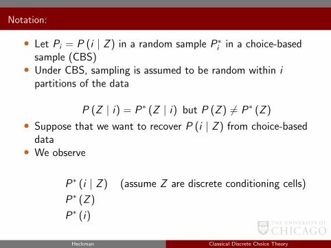
Notation:
• Let Pi = P (i | Z ) in a random sample P∗i in a choice-basedsample (CBS)• Under CBS, sampling is assumed to be random within i
partitions of the data
P (Z | i) = P∗ (Z | i) but P (Z ) 6= P∗ (Z )
• Suppose that we want to recover P (i | Z ) from choice-baseddata• We observe
P∗ (i | Z ) (assume Z are discrete conditioning cells)
P∗ (Z )
P∗ (i)
Frequency weights :
P∗ (Z | i) = P (Z | i) (key assumption)
Heckman Classical Discrete Choice Theory
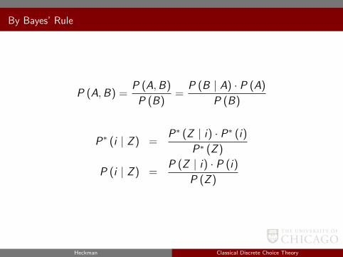
By Bayes’ Rule
P (A,B) =P (A,B)
P (B)=
P (B | A) · P (A)
P (B)
P∗ (i | Z ) =P∗ (Z | i) · P∗ (i)
P∗ (Z )
P (i | Z ) =P (Z | i) · P (i)
P (Z )
Heckman Classical Discrete Choice Theory
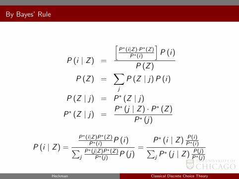
By Bayes’ Rule
P (i | Z ) =
[P∗(i |Z)·P∗(Z)
P∗(i)
]P (i)
P (Z )
P (Z ) =∑j
P (Z | j)P (i)
P (Z | j) = P∗ (Z | j)
P∗ (Z | j) =P∗ (j | Z ) · P∗ (Z )
P∗ (j)
P (i | Z ) =
P∗(i |Z)P∗(Z)P∗(i)
P (i)∑jP∗(j |Z)P∗(Z)
P∗(j)P (j)
=P∗ (i | Z ) P(i)
P∗(i)∑j P∗ (j | Z ) P(j)
P∗(j)
Heckman Classical Discrete Choice Theory
• To recover P (i | Z ) from choice-based sampled data, you needto know P (j) , P∗ (j) ∀j . P∗ (j) can be estimated from sample,
but P (j) requires outside information. Need weights P(i)P∗(i)
.
• Note: Problem set asks you to consider how CBS biases thecoefficients and intercept in a logit model. (Can show that biasonly in the constant)
Heckman Classical Discrete Choice Theory

Application and Extension: Berry, Levinsohn, and Pakes (1995)
• Develop equilibrium model and estimation techniques foranalyzing demand and supply in differentiated product markets
• Use to study automobile industry
• Goal is to estimate parameters of both the demand and costfunctions incorporating own and cross price elasticities andelasticities with respect to product attributes (car horse power,MPG, air conditioning, size,...) using only aggregate productlevel data supplemented with data on consumer characteristicdistributions (income distribution from CBS)
• Want to allow for flexible substitution patterns
Heckman Classical Discrete Choice Theory

Key assumptions
(i) joint distribution of observed and unobserved product andconsumer characteristics
(ii) price taking for consumers, Nash eq assumptions on producersin oligopolistic, differentiated products market.
Heckman Classical Discrete Choice Theory
Notation
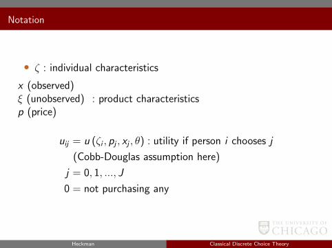
• ζ : individual characteristics
x (observed)ξ (unobserved)p (price)
: product characteristics
uij = u (ζi , pj , xj , θ) : utility if person i chooses j
(Cobb-Douglas assumption here)
j = 0, 1, ..., J
0 = not purchasing any
Heckman Classical Discrete Choice Theory

Notation
• Define
Aj = ζ : uij (ζ, pj , xj , ξj ; θ) ≥ u (ζ, pr , xr , ξr ; 0) r = 0, ..., J ,
• the set of ζ that induces choice of good j . This is defined overindividual characteristics which may be observed or unobserved.
Heckman Classical Discrete Choice Theory
Market Share
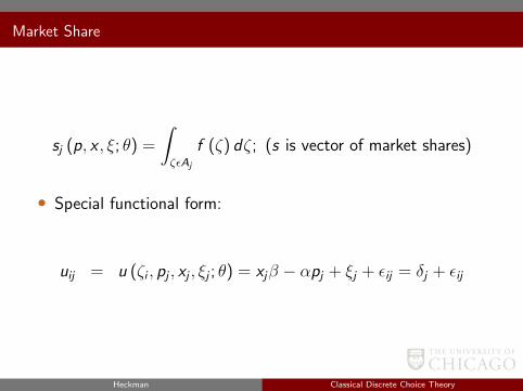
sj (p, x , ξ; θ) =
∫ζεAj
f (ζ) dζ; (s is vector of market shares)
• Special functional form:
uij = u (ζi , pj , xj , ξj ; θ) = xjβ − αpj + ξj + εij = δj + εij
Heckman Classical Discrete Choice Theory
Market Share
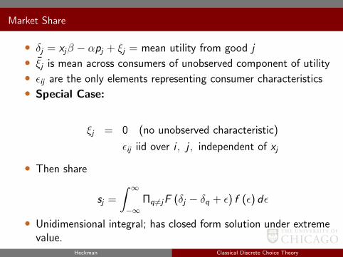
• δj = xjβ − αpj + ξj = mean utility from good j• ξj is mean across consumers of unobserved component of utility• εij are the only elements representing consumer characteristics• Special Case:
ξj = 0 (no unobserved characteristic)
εij iid over i , j , independent of xj
• Then share
sj =
∫ ∞−∞
Πq 6=jF (δj − δq + ε) f (ε) dε
• Unidimensional integral; has closed form solution under extremevalue.
Heckman Classical Discrete Choice Theory
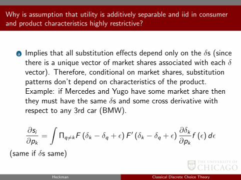
Why is assumption that utility is additively separable and iid in consumerand product characteristics highly restrictive?
(a) Implies that all substitution effects depend only on the δs (sincethere is a unique vector of market shares associated with each δvector). Therefore, conditional on market shares, substitutionpatterns don’t depend on characteristics of the product.Example: if Mercedes and Yugo have some market share thenthey must have the same δs and some cross derivative withrespect to any 3rd car (BMW).
∂si∂pk
=
∫Πq 6=kF (δk − δq + ε)F ′ (δk − δq + ε)
∂δk∂pk
f (ε) dε
(same if δs same)
Heckman Classical Discrete Choice Theory

Why is assumption that utility is additively separable and iid in consumerand product characteristics highly restrictive?
(b) Two products with same market share have same own pricederivatives (not good because you expect product markup todepend on more than market share)
(b) Also assumes that individuals value product characteristics insame way (no preference heterogeneity)
Heckman Classical Discrete Choice Theory
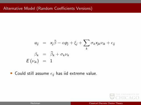
Alternative Model (Random Coefficients Versions)
uij = xj β − αpj + ξj +∑k
σkxjkνik + εij
βk = βk + σkνk
E (νik) = 1
• Could still assume εij has iid extreme value.
Heckman Classical Discrete Choice Theory
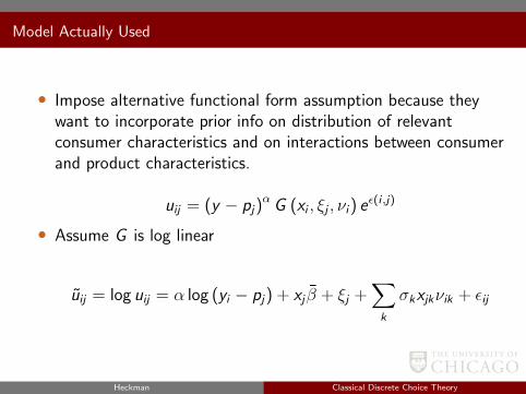
Model Actually Used
• Impose alternative functional form assumption because theywant to incorporate prior info on distribution of relevantconsumer characteristics and on interactions between consumerand product characteristics.
uij = (y − pj)α G (xi , ξj , νi) e
ε(i ,j)
• Assume G is log linear
uij = log uij = α log (yi − pj) + xj β + ξj +∑k
σkxjkνik + εij
Heckman Classical Discrete Choice Theory
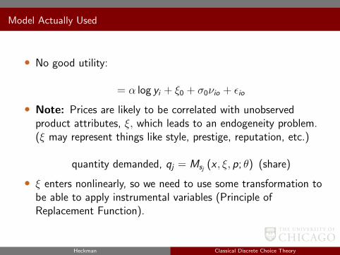
Model Actually Used
• No good utility:
= α log yi + ξ0 + σ0νio + εio
• Note: Prices are likely to be correlated with unobservedproduct attributes, ξ, which leads to an endogeneity problem.(ξ may represent things like style, prestige, reputation, etc.)
quantity demanded, qj = Msj (x , ξ, p; θ) (share)
• ξ enters nonlinearly, so we need to use some transformation tobe able to apply instrumental variables (Principle ofReplacement Function).
Heckman Classical Discrete Choice Theory
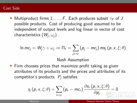
Cost Side
• Multiproduct firms 1, . . . ,F . Each produces subset τF of Jpossible products. Cost of producing good assumed to beindependent of output levels and log linear in vector of costcharacteristics (Wj , ωj) .
lnmcj = Wjγ + ωj ⇒ Πf =∑j∈τF
(pj −mcj)msj (p, x , ξ; θ)
Nash Assumption• Firm chooses prices that maximize profit taking as given
attributes of its products and the prices and attributes of itscompetitor’s products. Pj satisfies
sj (p, x , ξ; θ) +∑rετF
(pr −mcr )∂sr (p, x , ξ; θ)
∂pj= 0
Heckman Classical Discrete Choice Theory
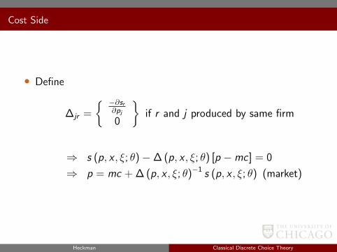
Cost Side
• Define
∆jr =
−∂sr∂pj
0
if r and j produced by same firm
⇒ s (p, x , ξ; θ)−∆ (p, x , ξ; θ) [p −mc] = 0
⇒ p = mc + ∆ (p, x , ξ; θ)−1 s (p, x , ξ; θ) (market)
Heckman Classical Discrete Choice Theory
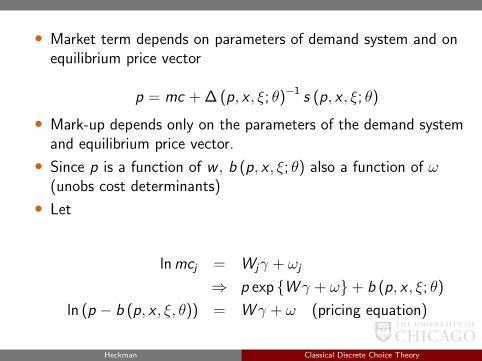
• Market term depends on parameters of demand system and onequilibrium price vector
p = mc + ∆ (p, x , ξ; θ)−1 s (p, x , ξ; θ)
• Mark-up depends only on the parameters of the demand systemand equilibrium price vector.
• Since p is a function of w , b (p, x , ξ; θ) also a function of ω(unobs cost determinants)
• Let
lnmcj = Wjγ + ωj
⇒ p exp W γ + ω+ b (p, x , ξ; θ)
ln (p − b (p, x , ξ, θ)) = W γ + ω (pricing equation)
Heckman Classical Discrete Choice Theory
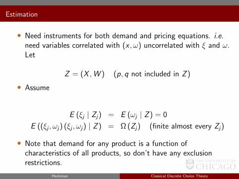
Estimation
• Need instruments for both demand and pricing equations. i.e.need variables correlated with (x , ω) uncorrelated with ξ and ω.Let
Z = (X ,W ) (p, q not included in Z )
• Assume
E (ξj | Zj) = E (ωj | Z ) = 0
E ((ξj , ωj) (ξj , ωj) | Z ) = Ω (Zj) (finite almost every Zj)
• Note that demand for any product is a function ofcharacteristics of all products, so don’t have any exclusionrestrictions.
Heckman Classical Discrete Choice Theory
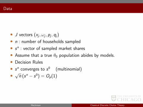
Data
• J vectors (xj , ωj , pj , qj)
• n : number of households sampled
• sn : vector of sampled market shares
• Assume that a true θ0 population abides by models.
• Decision Rules
• sn converges to s0 (multinomial)
• √n (sn − s0) = Op(1)
Heckman Classical Discrete Choice Theory
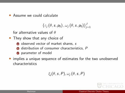
• Assume we could calculate
εj (θ, s, p0) , ωj (θ, s, p0)Jj=1
for alternative values of θ
• They show that any choice of
(a) observed vector of market shares, s(b) distribution of consumer characteristics, P(c) parameter of model
• implies a unique sequence of estimates for the two unobservedcharacteristics
ξj(θ, s,P), ωj (θ, s,P)
Heckman Classical Discrete Choice Theory
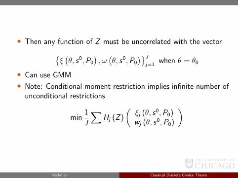
• Then any function of Z must be uncorrelated with the vectorξ(θ, s0,P0
), ω(θ, s0,P0
)Jj=1
when θ = θ0
• Can use GMM
• Note: Conditional moment restriction implies infinite number ofunconditional restrictions
min1
J
∑Hj (Z )
(ξj (θ, s0,P0)wj (θ, s0,P0)
)
Heckman Classical Discrete Choice Theory
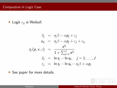
Compuation in Logit Case
• Logit εij is Weibull.
δj = xjβ − αpj + εj
uij = xjβ − αpj + εj + εij
sj (p, x , ε) =eδj
1 +∑J
j=1 eδj
δj = ln sj − ln s0, j = 1, . . . , J
εj = ln sj − ln s0 − xjβ + αpj
• See paper for more details.
Heckman Classical Discrete Choice Theory

Generalized Method of Moments (GMM)
References:• Hansen (1982), Econometrica• Hansen and Singleton (1982,1988)• Also known as “minimum distance estimators”• Suppose that we have some data xt t = 1...T and we want
to test hypotheses about E (xt = µ) .• How do we proceed? By a CLT
1√T
T∑t=1
(xt − µ) ∼ N (O,V0)
V0 = E((xt − µ) (xt − µ)′
)if xt iid
= limt→∞
E
(1√Tv∑t
(xt − µ)1√T
(xt − µ)′)
(general case)
Heckman Classical Discrete Choice Theory
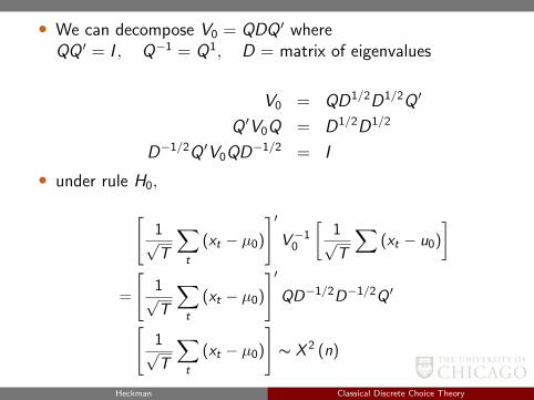
• We can decompose V0 = QDQ ′ whereQQ ′ = I , Q−1 = Q1, D = matrix of eigenvalues
V0 = QD1/2D1/2Q ′
Q ′V0Q = D1/2D1/2
D−1/2Q ′V0QD−1/2 = I
• under rule H0,[1√T
∑t
(xt − µ0)
]′V−1
0
[1√T
∑(xt − u0)
]
=
[1√T
∑t
(xt − µ0)
]′QD−1/2D−1/2Q ′[
1√T
∑t
(xt − µ0)
]∼ X 2 (n)
Heckman Classical Discrete Choice Theory
• where n is the number of moment conditions.
• How does test statistic behave under alternative? (µ 6= µ0)
• should get large
Heckman Classical Discrete Choice Theory
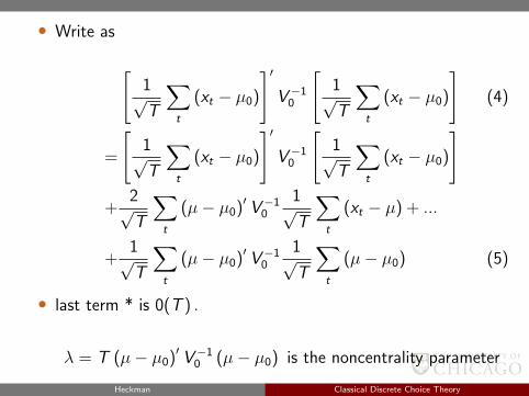
• Write as
[1√T
∑t
(xt − µ0)
]′V−1
0
[1√T
∑t
(xt − µ0)
](4)
=
[1√T
∑t
(xt − µ0)
]′V−1
0
[1√T
∑t
(xt − µ0)
]+
2√T
∑t
(µ− µ0)′ V−10
1√T
∑t
(xt − µ) + ...
+1√T
∑t
(µ− µ0)′ V−10
1√T
∑t
(µ− µ0) (5)
• last term * is 0(T ) .
λ = T (µ− µ0)′ V−10 (µ− µ0) is the noncentrality parameter
Heckman Classical Discrete Choice Theory
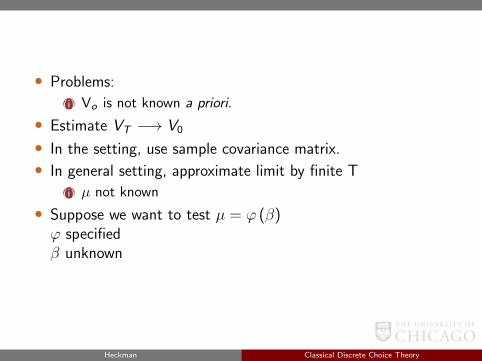
• Problems:
(i) Vo is not known a priori.
• Estimate VT −→ V0
• In the setting, use sample covariance matrix.
• In general setting, approximate limit by finite T
(i) µ not known
• Suppose we want to test µ = ϕ (β)ϕ specifiedβ unknown
Heckman Classical Discrete Choice Theory
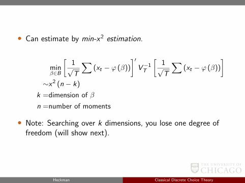
• Can estimate by min-x2 estimation.
minβ∈B
[1√T
∑(xt − ϕ (β))
]′V−1T
[1√T
∑(xt − ϕ (β))
]∼x2 (n − k)
k =dimension of β
n =number of moments
• Note: Searching over k dimensions, you lose one degree offreedom (will show next).
Heckman Classical Discrete Choice Theory
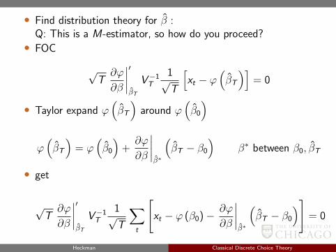
• Find distribution theory for β :Q: This is a M-estimator, so how do you proceed?• FOC
√T∂ϕ
∂β
∣∣∣∣′βT
V−1T
1√T
[xt − ϕ
(βT
)]= 0
• Taylor expand ϕ(βT
)around ϕ
(β0
)ϕ(βT
)= ϕ
(β0
)+∂ϕ
∂β
∣∣∣∣β∗
(βT − β0
)β∗ between β0, βT
• get
√T∂ϕ
∂β
∣∣∣∣′βT
V−1T
1√T
∑t
[xt − ϕ (β0)− ∂ϕ
∂β
∣∣∣∣β∗
(βT − β0
)]= 0
Heckman Classical Discrete Choice Theory
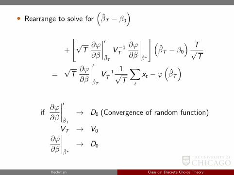
• Rearrange to solve for(βT − β0
)
+
[√T∂ϕ
∂β
∣∣∣∣′βT
V−1T
∂ϕ
∂β
∣∣∣∣β∗
](βT − β0
) T√T
=√T∂ϕ
∂β
∣∣∣∣′βT
V−1T
1√T
∑t
xt − ϕ(βT
)
if∂ϕ
∂β
∣∣∣∣′βT
→ D0 (Convergence of random function)
VT → V0
∂ϕ
∂β
∣∣∣∣β∗→ D0
Heckman Classical Discrete Choice Theory
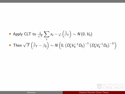
• Apply CLT to 1√T
∑t
xt − ϕ(βT
)∼ N (0,V0)
• Then√T(βT − β0
)∼ N
(0,(D ′0V
−10 D0
)−1 (D ′0V
−10 D0
)−1′)
Heckman Classical Discrete Choice Theory
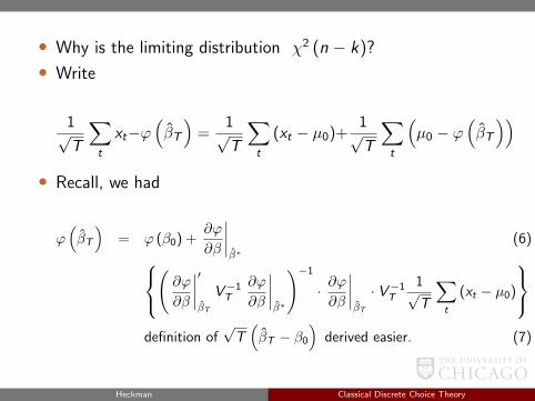
• Why is the limiting distribution χ2 (n − k)?
• Write
1√T
∑t
xt−ϕ(βT
)=
1√T
∑t
(xt − µ0)+1√T
∑t
(µ0 − ϕ
(βT
))• Recall, we had
ϕ(βT
)= ϕ (β0) +
∂ϕ
∂β
∣∣∣∣β∗
(6)(∂ϕ
∂β
∣∣∣∣′βT
V−1T
∂ϕ
∂β
∣∣∣∣β∗
)−1
· ∂ϕ∂β
∣∣∣∣βT
· V−1T
1√T
∑t
(xt − µ0)
definition of
√T(βT − β0
)derived easier. (7)
Heckman Classical Discrete Choice Theory
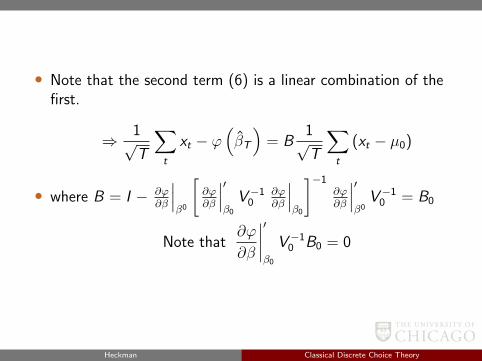
• Note that the second term (6) is a linear combination of thefirst.
⇒ 1√T
∑t
xt − ϕ(βT
)= B
1√T
∑t
(xt − µ0)
• where B = I − ∂ϕ∂β
∣∣∣β0
[∂ϕ∂β
∣∣∣′β0
V−10
∂ϕ∂β
∣∣∣β0
]−1∂ϕ∂β
∣∣∣′β0V−1
0 = B0
Note that∂ϕ
∂β
∣∣∣∣′β0
V−10 B0 = 0
Heckman Classical Discrete Choice Theory
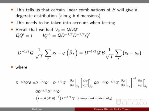
• This tells us that certain linear combinations of B will give adegerate distribution (along k dimensions)
• This needs to be taken into account when testing.
• Recall that we had V0 = QDQ ′
QQ ′ = I V−10 = QD−1/2D−1/2Q ′
D−1/2Q ′1√T
∑t
xt − ϕ(βT
)= D−1/2Q ′B
1√T
∑t
(xt − µ0)
• where
D−1/2Q′B =D−1/2Q′ − D−1/2Q′ ·∂ϕ
∂β
∣∣∣∣βT
[∂ϕ
∂β
∣∣∣∣′βT
QD−1/2D−1/2Q′∂ϕ
∂β
∣∣∣∣βT
]−1∂ϕ
∂β
∣∣∣∣′β0
QD−1/2D−1/2Q′
=(I − A
(A′A
)−1)D−1/2Q′ (idempotent matrix MA)
Heckman Classical Discrete Choice Theory
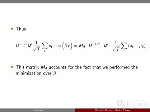
• Thus
D−1/2Q ′1√T
∑t
xt − ϕ(βT
)= MA · D−1/2 · Q ′ · 1√
T
∑t
(xt − µ0)
• This matrix MA accounts for the fact that we performed theminimization over β
Heckman Classical Discrete Choice Theory
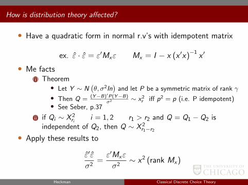
How is distribution theory affected?
• Have a quadratic form in normal r.v’s with idempotent matrix
ex. ε · ε = ε′Mxε Mx = I − x (x ′x)−1
x ′
• Me facts(i) Theorem
• Let Y ∼ N(θ, σ2In
)and let P be a symmetric matrix of rank γ
• Then Q = (Y−B)′P(Y−B)σ2 ∼ x2
r iff p2 = p (i.e. P idempotent)• See Seber, p.37
(ii) if Qi ∼ X 2ri
i = 1, 2 r1 > r2 and Q = Q1 − Q2 isindependent of Q2, then Q ∼ X 2
r1−r2
• Apply these results to
ε′ε
σ2=ε′Mxε
σ2∼ x2 (rank Mx)
Heckman Classical Discrete Choice Theory
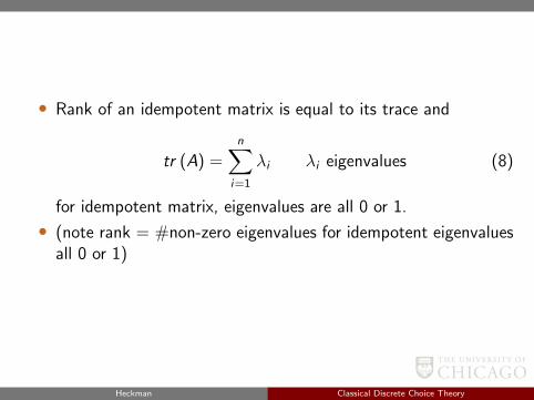
• Rank of an idempotent matrix is equal to its trace and
tr (A) =n∑
i=1
λi λi eigenvalues (8)
for idempotent matrix, eigenvalues are all 0 or 1.
• (note rank = #non-zero eigenvalues for idempotent eigenvaluesall 0 or 1)
Heckman Classical Discrete Choice Theory
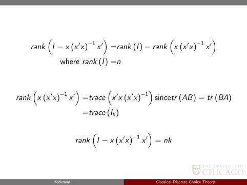
rank(I − x (x ′x)
−1x ′)
=rank (I )− rank(x (x ′x)
−1x ′)
where rank (I ) =n
rank(x (x ′x)
−1x ′)
=trace(x ′x (x ′x)
−1)
sincetr (AB) = tr (BA)
=trace (Ik)
rank(I − x (x ′x)
−1x ′)
= nk
Heckman Classical Discrete Choice Theory
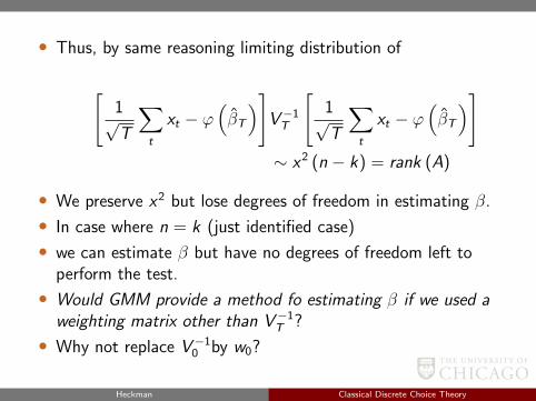
• Thus, by same reasoning limiting distribution of
[1√T
∑t
xt − ϕ(βT
)]V−1T
[1√T
∑t
xt − ϕ(βT
)]∼ x2 (n − k) = rank (A)
• We preserve x2 but lose degrees of freedom in estimating β.
• In case where n = k (just identified case)
• we can estimate β but have no degrees of freedom left toperform the test.
• Would GMM provide a method fo estimating β if we used aweighting matrix other than V−1
T ?
• Why not replace V−10 by w0?
Heckman Classical Discrete Choice Theory
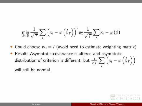
minβ∈B
1√T
∑t
(xt − ϕ
(βT
))′w0
1√T
∑t
xt − ϕ (β)
• Could choose w0 = I (avoid need to estimate weighting matrix)
• Result: Asymptotic covariance is altered and asymptotic
distribution of criterion is different, but 1√T
∑t
(xt − ϕ
(βT
))will still be normal.
Heckman Classical Discrete Choice Theory
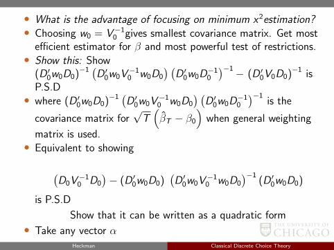
• What is the advantage of focusing on minimum x2estimation?• Choosing w0 = V−1
0 gives smallest covariance matrix. Get mostefficient estimator for β and most powerful test of restrictions.• Show this: Show
(D ′0w0D0)−1 (D ′0w0V−10 w0D0
) (D ′0w0D
−10
)−1− (D ′0V0D0)−1 isP.S.D• where (D ′0w0D0)−1 (D ′0w0V
−10 w0D0
) (D ′0w0D
−10
)−1is the
covariance matrix for√T(βT − β0
)when general weighting
matrix is used.• Equivalent to showing
(D0V
−10 D0
)− (D ′0w0D0)
(D ′0w0V
−10 w0D0
)−1(D ′0w0D0)
is P.S.D
Show that it can be written as a quadratic form
• Take any vector αHeckman Classical Discrete Choice Theory
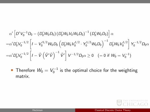
α′[D ′V−1
0 D0 − (D ′0W0D0) (D ′0W0V0W0D0)−1
(D ′0W0D0)]α
=α′D ′0V−1/20
[I − V
′1/20 W0D0
(D ′0W0V
1/20 · Y 1/2
0 W0D0
)−1
D ′0W0V1/20
]Y−1/20 D0α
=α′D ′0V−1/20
[I − V
(V ′V
)−1
V ′]V−1/2D0α ≥ 0 (= 0 if W0 = V−1
0 )
• Therefore W0 = V−10 is the optimal choice for the weighting
matrix.
Heckman Classical Discrete Choice Theory
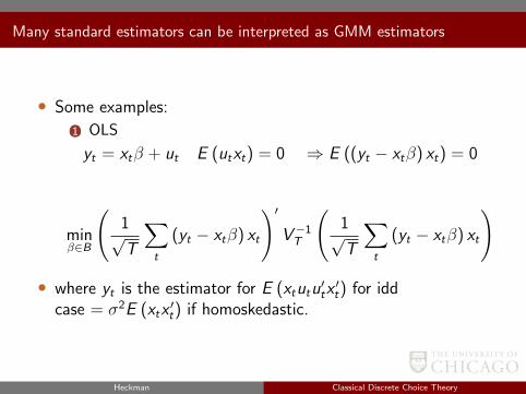
Many standard estimators can be interpreted as GMM estimators
• Some examples:
(1) OLS
yt = xtβ + ut E (utxt) = 0 ⇒ E ((yt − xtβ) xt) = 0
minβ∈B
(1√T
∑t
(yt − xtβ) xt
)′V−1T
(1√T
∑t
(yt − xtβ) xt
)
• where yt is the estimator for E (xtutu′tx′t) for idd
case = σ2E (xtx′t) if homoskedastic.
Heckman Classical Discrete Choice Theory
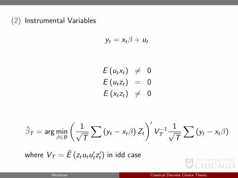
(2) Instrumental Variables
yt = xtβ + ut
E (utxt) 6= 0
E (utzt) = 0
E (xtzt) 6= 0
βT = arg minβ∈B
(1√T
∑(yt − xtβ)Zt
)′V−1T
1√T
∑(yt − xtβ)
where VT = E (ztutu′tz′t) in idd case
Heckman Classical Discrete Choice Theory
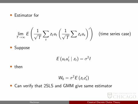
• Estimator for
limT→∞
E
(1√T
∑t
ztut
(1√T
∑zsus
)′)(time series case)
• Suppose
E (utu′t | zt) = σ2I
• then
W0 = σ2E (ztz′t)
• Can verify that 2SLS and GMM give same estimator
Heckman Classical Discrete Choice Theory
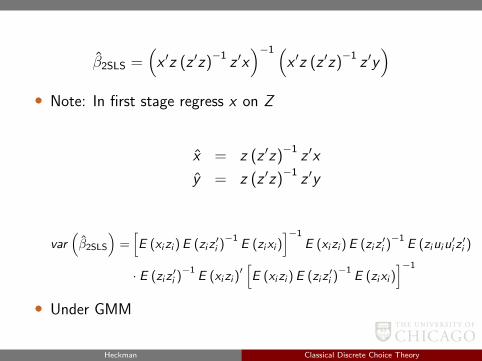
β2SLS =(x ′z (z ′z)
−1z ′x)−1 (
x ′z (z ′z)−1
z ′y)
• Note: In first stage regress x on Z
x = z (z ′z)−1
z ′x
y = z (z ′z)−1
z ′y
var(β2SLS
)=[E (xizi )E (ziz
′i )−1
E (zixi )]−1
E (xizi )E (ziz′i )−1
E (ziuiu′i z′i )
· E (ziz′i )−1
E (xizi )′[E (xizi )E (ziz
′i )−1
E (zixi )]−1
• Under GMM
Heckman Classical Discrete Choice Theory

var(βGMM
)=
(D0V
−10 D0
)−1(when W0 = V−1
0 )
D0 =∂ϕ
∂β|β0= p lim
1n
∑xiz
′
i = E (xiz′i )
W0 =(σ2)−1
E (ziz′i )−1
Heckman Classical Discrete Choice Theory
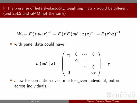
In the presense of heterskedastocity, weighting matrix would be different(and 2SLS and GMM not the same)
W0 = E (z ′uu′z)−1
= E (z ′E (uu′ | z) z)−1
= E (z ′vz)−1
• with panel data could have
E (uu′ | z) =
v1 0 · · · 0
v2 · · ·. . . 0
0 vT
= y
• allow for correlation over time for given individual, but iidacross individuals.
Heckman Classical Discrete Choice Theory
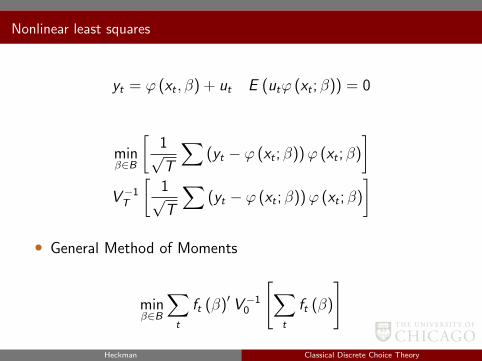
Nonlinear least squares
yt = ϕ (xt , β) + ut E (utϕ (xt ; β)) = 0
minβ∈B
[1√T
∑(yt − ϕ (xt ; β))ϕ (xt ; β)
]V−1T
[1√T
∑(yt − ϕ (xt ; β))ϕ (xt ; β)
]• General Method of Moments
minβ∈B
∑t
ft (β)′ V−10
[∑t
ft (β)
]
Heckman Classical Discrete Choice Theory
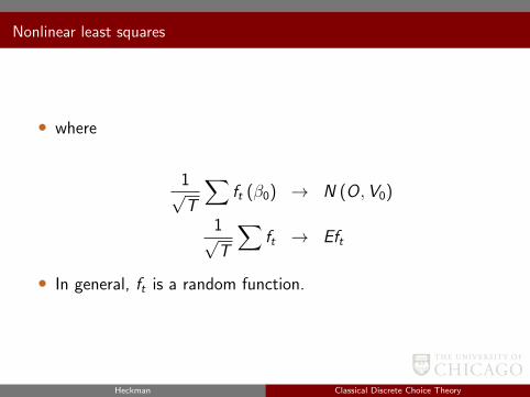
Nonlinear least squares
• where
1√T
∑ft (β0) → N (O,V0)
1√T
∑ft → Eft
• In general, ft is a random function.
Heckman Classical Discrete Choice Theory
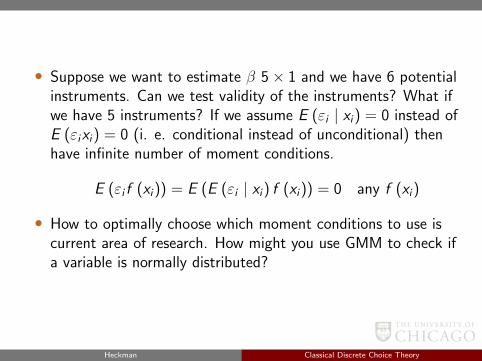
• Suppose we want to estimate β 5× 1 and we have 6 potentialinstruments. Can we test validity of the instruments? What ifwe have 5 instruments? If we assume E (εi | xi) = 0 instead ofE (εixi) = 0 (i. e. conditional instead of unconditional) thenhave infinite number of moment conditions.
E (εi f (xi)) = E (E (εi | xi) f (xi)) = 0 any f (xi)
• How to optimally choose which moment conditions to use iscurrent area of research. How might you use GMM to check ifa variable is normally distributed?
Heckman Classical Discrete Choice Theory

Return to main text
Heckman Classical Discrete Choice Theory