104/20/23 Inference about µ 1

Chapter 17

Inference about a Population Mean

204/20/23 Inference about µ 2

σ not known

nsSEx

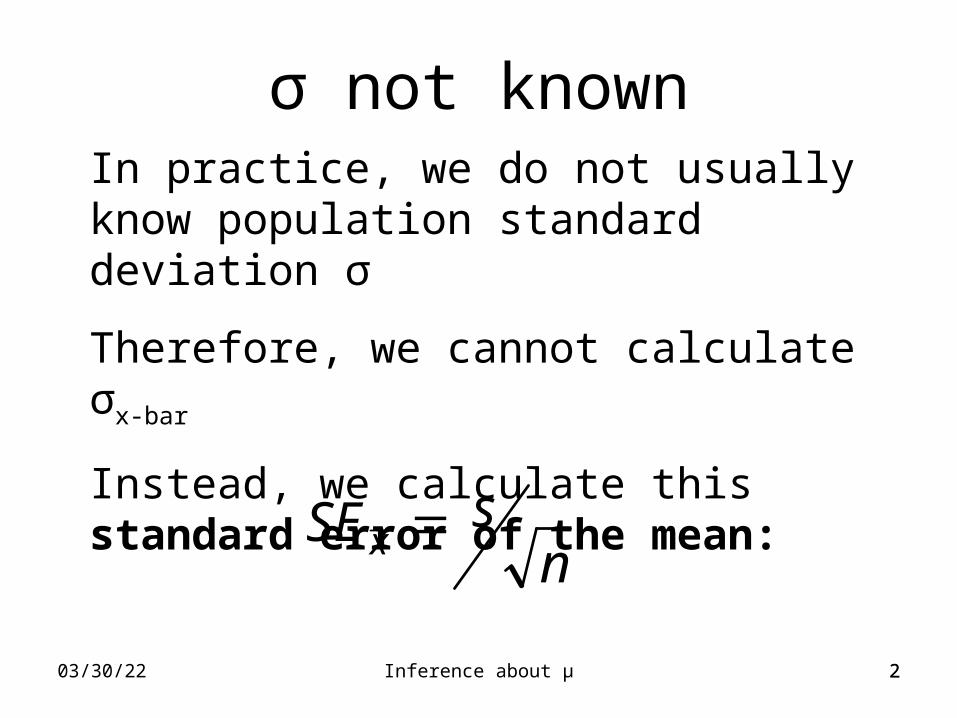
In practice, we do not usually know population standard deviation σ

Therefore, we cannot calculate σx-bar

Instead, we calculate this standard error of the mean:

304/20/23 Inference about µ 3

t Procedures

ns

μxt

nσ

μxz 00

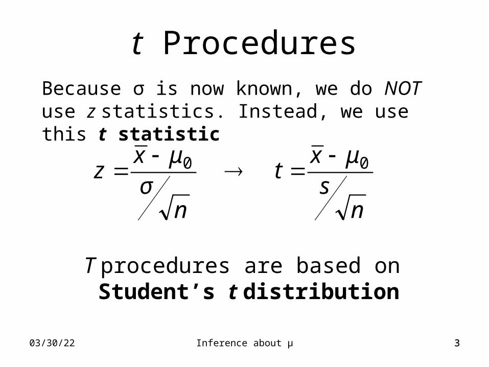
Because σ is now known, we do NOT use z statistics. Instead, we use this t statistic

T procedures are based on Student’s t distribution

404/20/23 Inference about µ 4

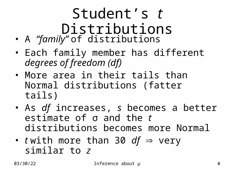
Student’s t Distributions• A “family” of distributions

• Each family member has different degrees of freedom (df)

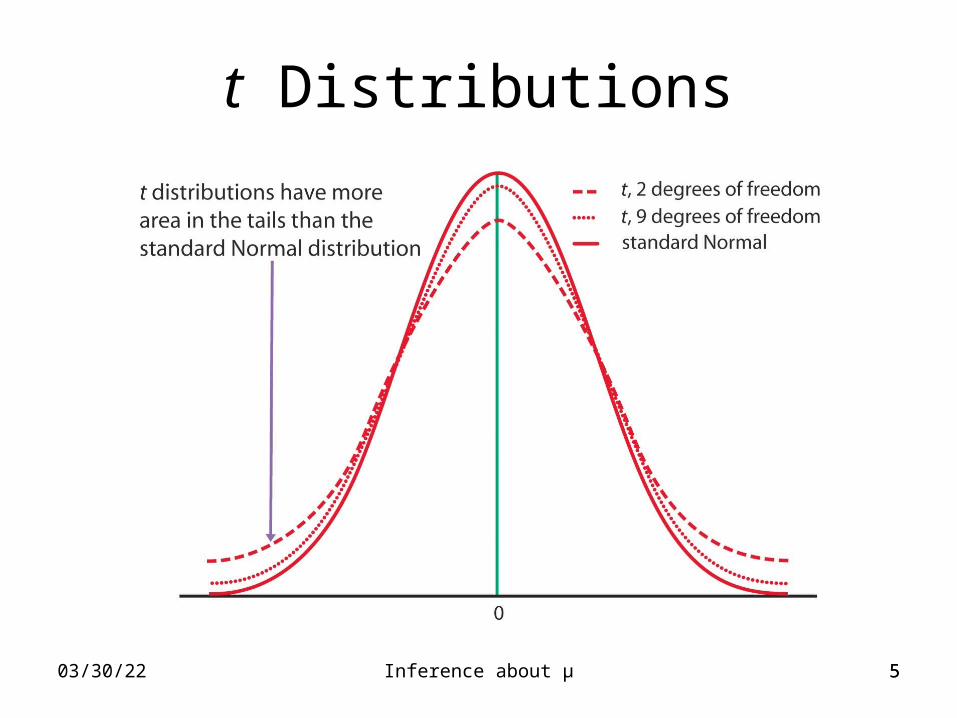
• More area in their tails than Normal distributions (fatter tails)

• As df increases, s becomes a better estimate of σ and the t distributions becomes more Normal

• t with more than 30 df very similar to z

504/20/23 Inference about µ 5

t Distributions

604/20/23 Inference about µ 6

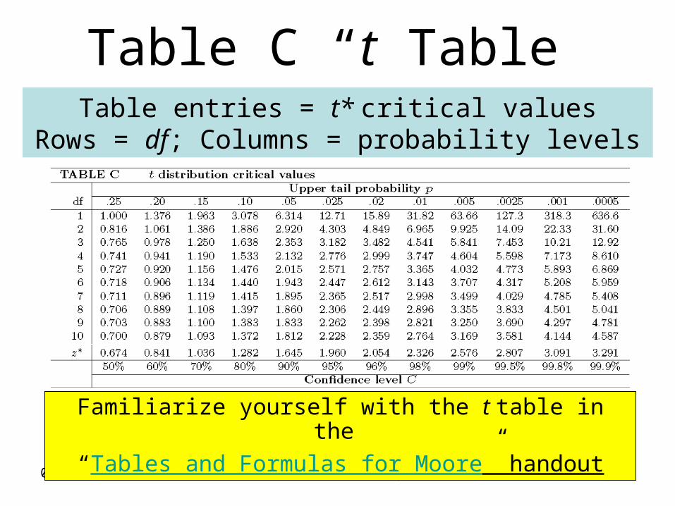
Table C “t Table”Table entries = t* critical values

Rows = df; Columns = probability levels

Familiarize yourself with the t table in the “Tables and Formulas for Moore” handout

704/20/23 Inference about µ 7

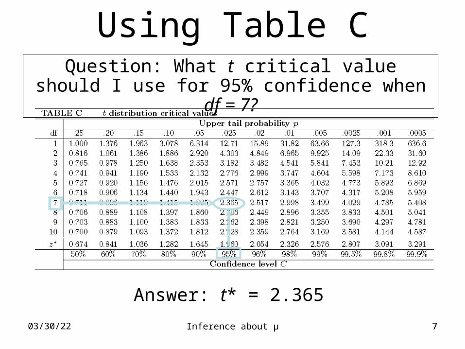
Using Table CQuestion: What t critical value should I use for

95% confidence when df = 7?

Answer: t* = 2.365

804/20/23 Inference about µ 8

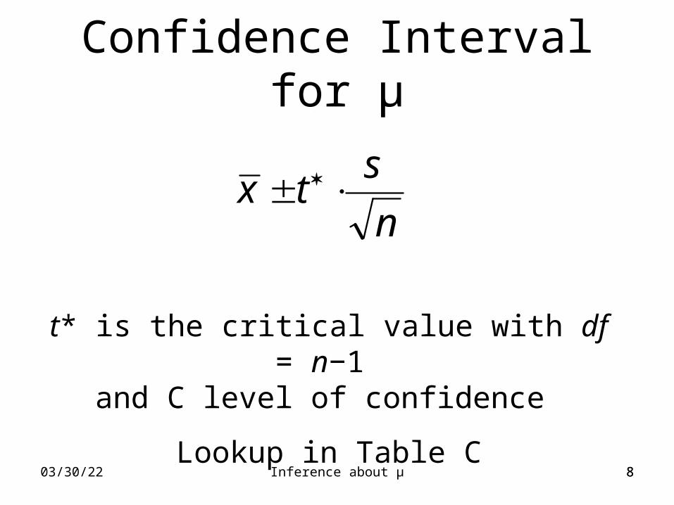
Confidence Interval for μ

n

stx

t* is the critical value with df = n−1 and C level of confidence

Lookup in Table C

9

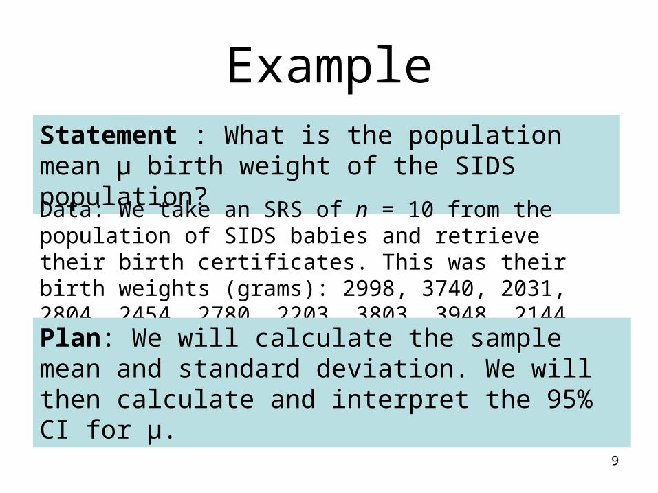
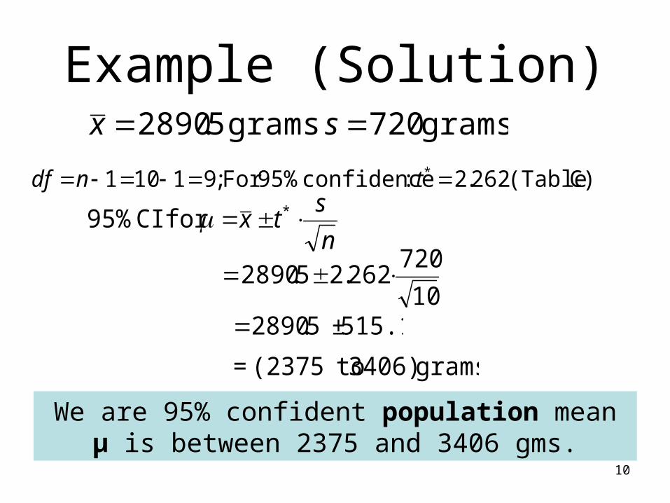
ExampleStatement : What is the population mean µ birth weight of the SIDS population?

Data: We take an SRS of n = 10 from the population of SIDS babies and retrieve their birth certificates. This was their birth weights (grams): 2998, 3740, 2031, 2804, 2454, 2780, 2203, 3803, 3948, 2144

Plan: We will calculate the sample mean and standard deviation. We will then calculate and interpret the 95% CI for µ.

10

Example (Solution)

n

stx * for CI 95%

C) (Table 262.2 :confidence 95%For ;91101 * tndf

grams 3406) to(2375 =

515.1 ±5.2890

We are 95% confident population mean µ is between 2375 and 3406 gms.

10

720262.25.2890

grams 720 grams 5.2890 sx

1104/20/23 Inference about µ 11

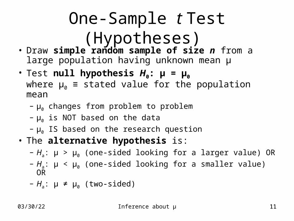
One-Sample t Test (Hypotheses) • Draw simple random sample of size n from a

large population having unknown mean µ• Test null hypothesis H0: μ = μ0

where μ0 ≡ stated value for the population mean– μ0 changes from problem to problem – μ0 is NOT based on the data– μ0 IS based on the research question

• The alternative hypothesis is:– Ha: μ > μ0 (one-sided looking for a larger value) OR– Ha: μ < μ0 (one-sided looking for a smaller value) OR– Ha: μ ≠ μ0 (two-sided)

1204/20/23 Inference about µ 12

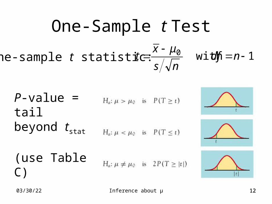
One-Sample t Test

1 with

ndfns

μxt 0One-sample t statistic:

P-value = tail beyond tstat (use Table C)

13Basics of Significance Testing 13

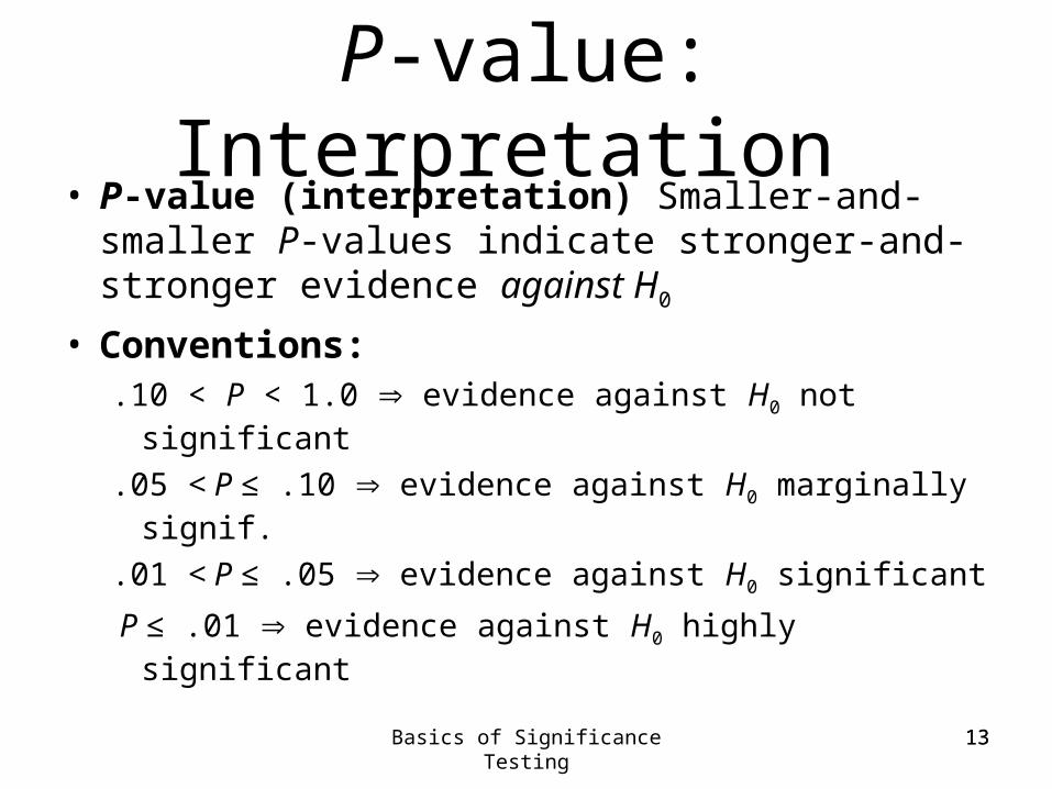
P-value: Interpretation • P-value (interpretation) Smaller-and-smaller P-

values indicate stronger-and-stronger evidence against H0

• Conventions:.10 < P < 1.0 evidence against H0 not significant

.05 < P ≤ .10 evidence against H0 marginally signif.

.01 < P ≤ .05 evidence against H0 significant

P ≤ .01 evidence against H0 highly significant

1404/20/23 Inference about µ 14

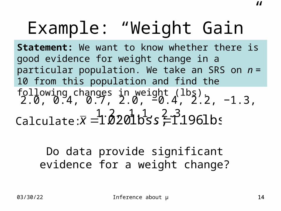
Statement: We want to know whether there is good evidence for weight change in a particular population. We take an SRS on n = 10 from this population and find the following changes in weight (lbs).

Example: “Weight Gain”

2.0, 0.4, 0.7, 2.0, −0.4, 2.2, −1.3, 1.2, 1.1, 2.3

lbs. 196.1 lbs.; 020.1 sxCalculate:

Do data provide significant evidence for a weight change?

1504/20/23 Inference about µ 15

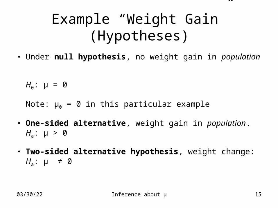
Example “Weight Gain” (Hypotheses)

• Under null hypothesis, no weight gain in population

H0: μ = 0

Note: µ0 = 0 in this particular example

• One-sided alternative, weight gain in population. Ha: μ > 0

• Two-sided alternative hypothesis, weight change:Ha: μ ≠ 0

1604/20/23 Inference about µ 16

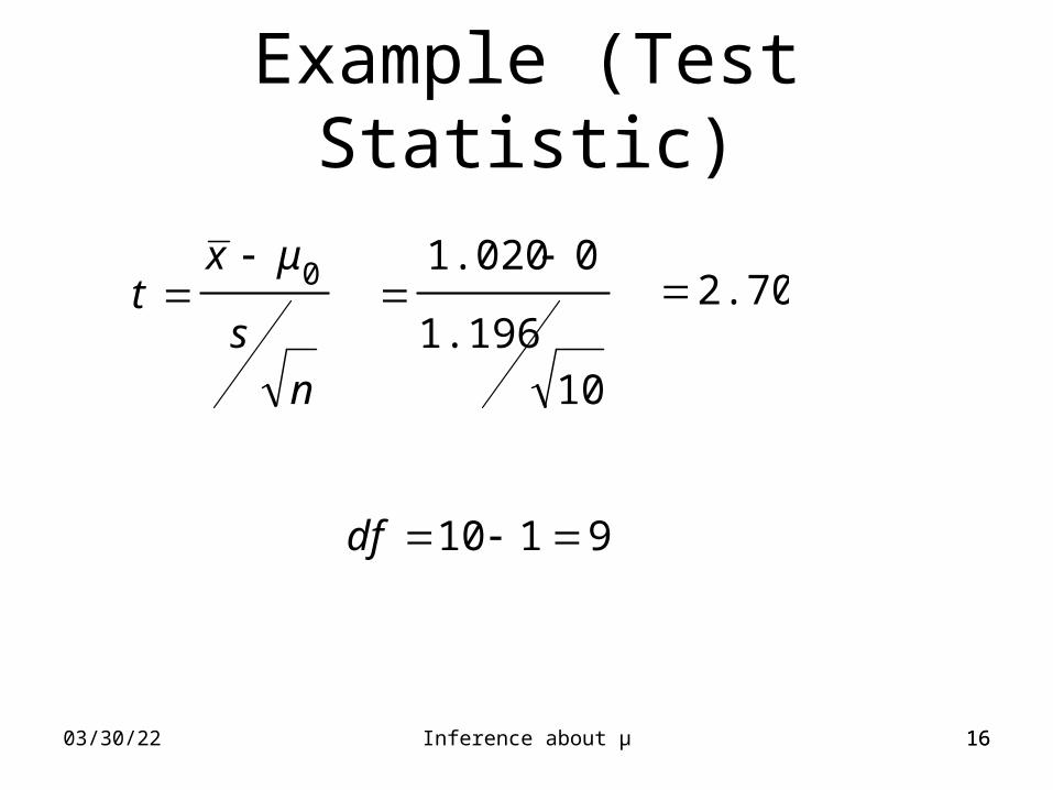
Example (Test Statistic)

9110 df

2.70

ns

μxt

0

101.196

01.020

1704/20/23 Inference about µ 17

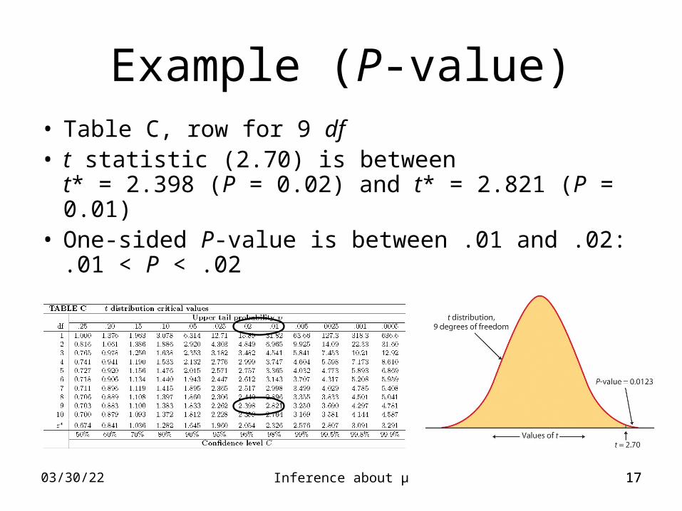
Example (P-value)• Table C, row for 9 df• t statistic (2.70) is between

t* = 2.398 (P = 0.02) and t* = 2.821 (P = 0.01) • One-sided P-value is between .01 and .02:

.01 < P < .02

18

Two-tailed P-value• For two-sided Ha,

P-value = 2 × one-sided P

• In our example, the one-tailed P-value was between .01 and .02

• Thus, the two-tailed P value is between .02 and .04

19

Interpretation• Interpret P-value in

context of claim made by H0

• In our example, H0: µ = 0 (no weight gain)

• Two-tailed P-value between .02 and .04

• Conclude: significant evidence against H0

2004/20/23 Inference about µ 20

Paired SamplesResponses in matched pairs

Parameter μ now represents the population mean difference

2104/20/23 Inference about µ 21

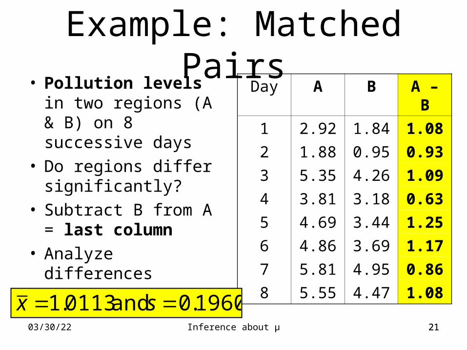
Example: Matched Pairs• Pollution levels in

two regions (A & B) on 8 successive days

• Do regions differ significantly?

• Subtract B from A = last column

• Analyze differences

Day A B A – B

1 2.92 1.84 1.08

2 1.88 0.95 0.93

3 5.35 4.26 1.09

4 3.81 3.18 0.63

5 4.69 3.44 1.25

6 4.86 3.69 1.17

7 5.81 4.95 0.86

8 5.55 4.47 1.08

1960.0 and 0113.1 sx

2204/20/23 Inference about µ 22

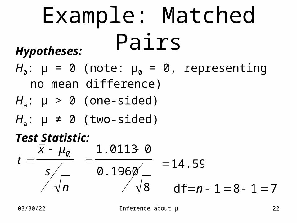
Hypotheses:

H0: μ = 0 (note: µ0 = 0, representing no mean difference)

Ha: μ > 0 (one-sided)

Ha: μ ≠ 0 (two-sided)

Test Statistic:

ns

μxt

0

Example: Matched Pairs

7181 n df80.1960

01.0113 14.59

2304/20/23 Inference about µ 23

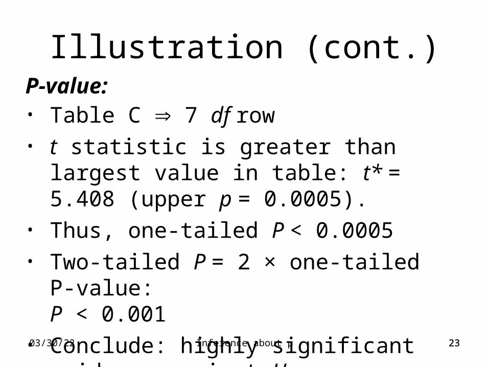
P-value: • Table C 7 df row

• t statistic is greater than largest value in table: t* = 5.408 (upper p = 0.0005).

• Thus, one-tailed P < 0.0005• Two-tailed P = 2 × one-tailed P-value:

P < 0.001 • Conclude: highly significant evidence

against H0

Illustration (cont.)

2404/20/23 Inference about µ 24

0.16391.0113

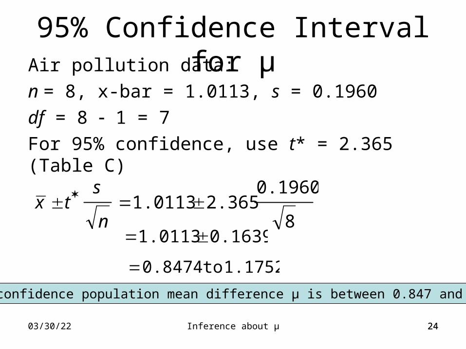
Air pollution data:

n = 8, x-bar = 1.0113, s = 0.1960

df = 8 1 = 7

For 95% confidence, use t* = 2.365 (Table C)

95% Confidence Interval for µ

8

0.19602.3651.0113

n

stx

1.1752 to 0.847495% confidence population mean difference µ is between 0.847 and 1.175

2504/20/23 Inference about µ 25

The confidence interval seeks population mean difference µ (IMPORTANT)

Recall the meaning of “confidence,” i.e., the ability of the interval to capture µ upon repetition

Recall from the prior chapter that the confidence interval can be used to address a null hypothesis

Interpreting the Confidence Interval

2604/20/23 Inference about µ 26

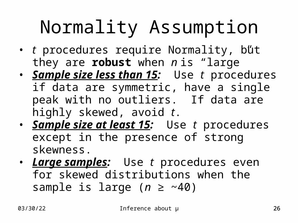
Normality Assumption• t procedures require Normality, but they are

robust when n is “large”• Sample size less than 15: Use t procedures if

data are symmetric, have a single peak with no outliers. If data are highly skewed, avoid t.

• Sample size at least 15: Use t procedures except in the presence of strong skewness.

• Large samples: Use t procedures even for skewed distributions when the sample is large (n ≥ ~40)

2704/20/23 Inference about µ 27

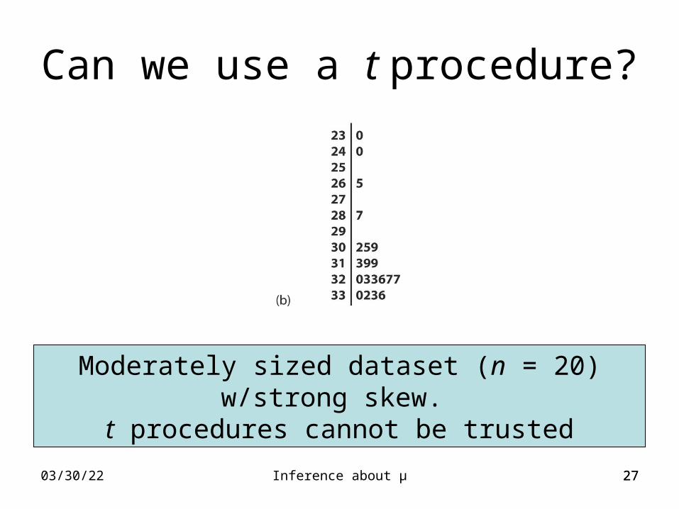
Can we use a t procedure?

Moderately sized dataset (n = 20) w/strong skew. t procedures cannot be trusted

2804/20/23 Inference about µ 28

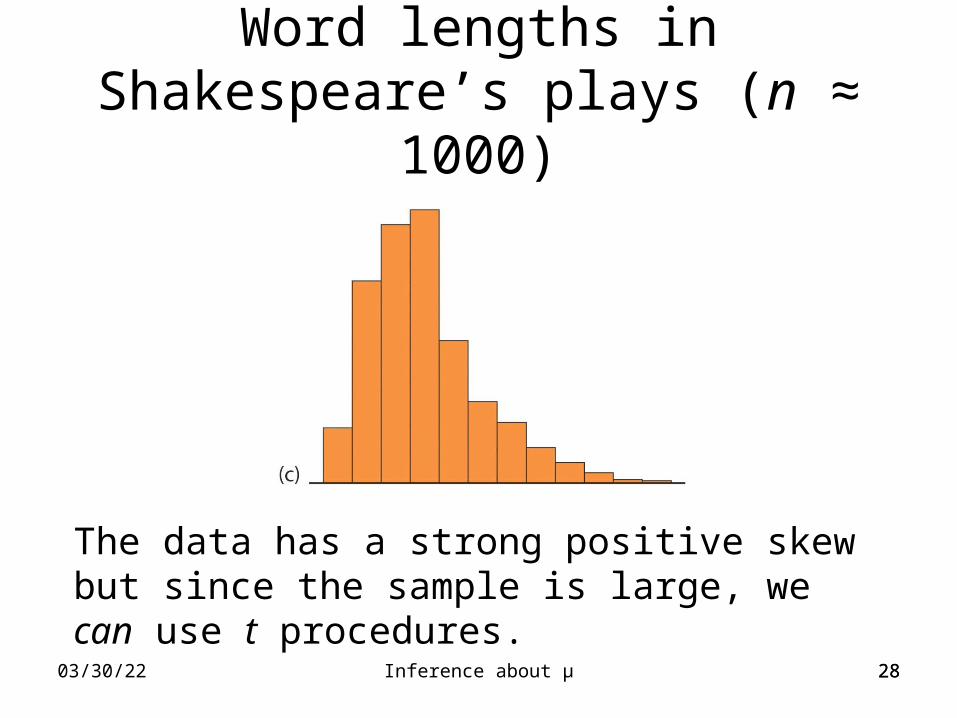
Word lengths in Shakespeare’s plays (n ≈ 1000)

The data has a strong positive skew but since the sample is large, we can use t procedures.

2904/20/23 Inference about µ 29

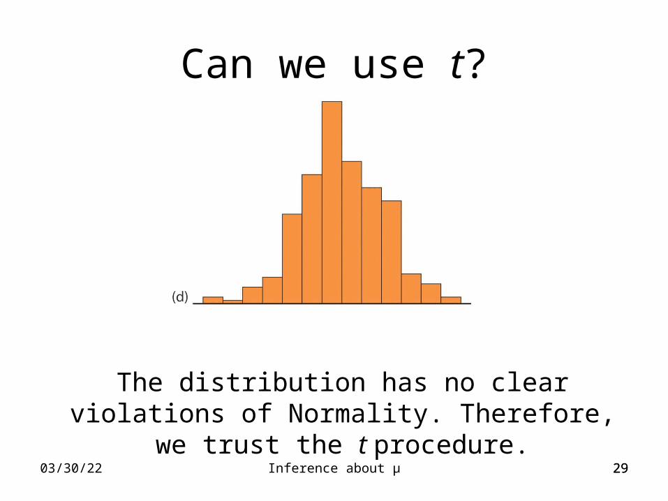
Can we use t?

The distribution has no clear violations of Normality. Therefore, we trust the t procedure.