![Mathematical Methods MATH30800marp/methods/... · E.g. 6.8: Find L[tsinat]. Since L[sinat] = a=(p2 + a2) (earlier E.g.) then L[tsinat] = d dp a p 2+ a 2ap (p2 + a2)2 6.4.3 Integrals](https://static.fdocument.org/doc/165x107/5f7c232aaec2254c4427dee5/mathematical-methods-math30800-marpmethods-eg-68-find-ltsinat-since.jpg)
Chapter 03 Mathematical Methods - University of...
17
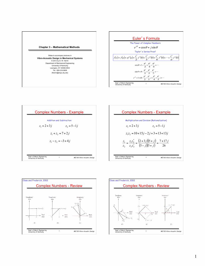
1 Slides to accompany lectures in Vibro-Acoustic Design in Mechanical Systems © 2012 by D. W. Herrin Department of Mechanical Engineering University of Kentucky Lexington, KY 40506-0503 Tel: 859-218-0609 [email protected] Chapter 3 – Mathematical Methods ME 510 Vibro-Acoustic Design Euler’s Formula θ θ θ sin cos j e j + = The Power of Complex Numbers () () () () () () () 0 ! 0 ! 4 0 ! 3 0 ! 2 4 4 3 3 2 2 1 n n f n x f x f x f x a xf a f x f + ⋅ ⋅ ⋅ + + + + + = Taylor’s Series Proof ⋅ ⋅ ⋅ + − + − = ! 6 ! 4 ! 2 1 cos 6 4 2 θ θ θ θ ⋅ ⋅ ⋅ + − + − = ! 7 ! 5 ! 3 sin 7 5 3 θ θ θ θ θ ⋅ ⋅ ⋅ + + + − − + = j j j e j ! 5 ! 4 ! 3 ! 2 1 5 4 3 2 θ θ θ θ θ θ Dept. of Mech. Engineering University of Kentucky 2 ME 510 Vibro-Acoustic Design Complex Numbers - Example j z 3 2 1 + = Addition and Subtraction j z z 2 7 2 1 + = + j z 1 5 2 − = j z z 4 3 2 1 + − = − Dept. of Mech. Engineering University of Kentucky 3 ME 510 Vibro-Acoustic Design Complex Numbers - Example j z 3 2 1 + = Multiplication and Division (Rationalization) j j j z z 13 13 3 2 15 10 2 1 + = + − + = j z 1 5 2 − = ( )( ) ( )( ) 26 17 7 5 5 5 3 2 * 2 2 * 2 1 2 1 j j j j j z z z z z z + = + − + + = = Dept. of Mech. Engineering University of Kentucky 4 ME 510 Vibro-Acoustic Design Complex Numbers - Review Close and Frederick, 2002 Dept. of Mech. Engineering University of Kentucky 5 ME 510 Vibro-Acoustic Design Complex Numbers - Review Close and Frederick, 2002 Dept. of Mech. Engineering University of Kentucky 6
Transcript of Chapter 03 Mathematical Methods - University of...
1
Slides to accompany lectures in
Vibro-Acoustic Design in Mechanical Systems © 2012 by D. W. Herrin
Department of Mechanical Engineering University of Kentucky
Lexington, KY 40506-0503 Tel: 859-218-0609
Chapter 3 – Mathematical Methods
ME 510 Vibro-Acoustic Design
Euler’s Formula
θθθ sincos je j +=
The Power of Complex Numbers
( ) ( ) ( ) ( ) ( ) ( ) ( )0!
0!4
0!3
0!2
44
33
22
1 nn
fnxfxfxfxaxfafxf +⋅⋅⋅+++++=
Taylor’s Series Proof
⋅⋅⋅+−+−=!6!4!2
1cos642 θθθ
θ
⋅⋅⋅+−+−=!7!5!3
sin753 θθθ
θθ
⋅⋅⋅+++−−+= jjje j!5!4!3!2
15432 θθθθ
θθ
Dept. of Mech. Engineering University of Kentucky
2
ME 510 Vibro-Acoustic Design
Complex Numbers - Example
jz 321 +=
Addition and Subtraction
jzz 2721 +=+
jz 152 −=
jzz 4321 +−=−
Dept. of Mech. Engineering University of Kentucky
3 ME 510 Vibro-Acoustic Design
Complex Numbers - Example
jz 321 +=
Multiplication and Division (Rationalization)
jjjzz 131332151021 +=+−+=
jz 152 −=
( )( )( )( ) 26
17755532
*22
*21
2
1 jjjjj
zzzz
zz +
=+−
++==
Dept. of Mech. Engineering University of Kentucky
4
ME 510 Vibro-Acoustic Design
Complex Numbers - Review Close and Frederick, 2002
Dept. of Mech. Engineering University of Kentucky
5 ME 510 Vibro-Acoustic Design
Complex Numbers - Review Close and Frederick, 2002
Dept. of Mech. Engineering University of Kentucky
6
2
ME 510 Vibro-Acoustic Design
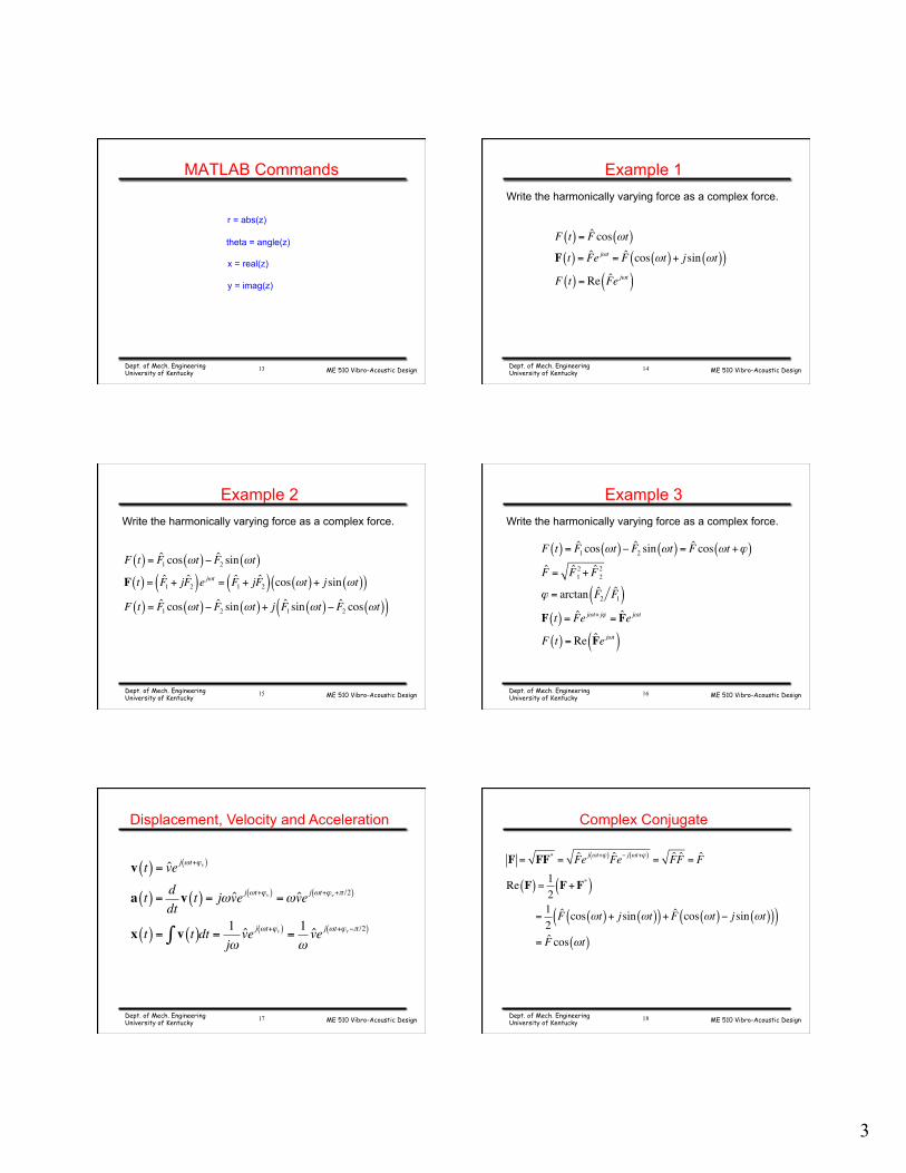
Polar Form - Review
θcoszx =θsinzy =
22 yxz +=
⎟⎠
⎞⎜⎝
⎛=xyarctanθ
θjezz =
Close and Frederick, 2002
Dept. of Mech. Engineering University of Kentucky
7 ME 510 Vibro-Acoustic Design
Complex Number Notations - Review
jyxz +=
( )θθ sincos jzz +=
θ∠= zzθjezz =
Rectangular Form
Polar Form
Close and Frederick, 2002
Dept. of Mech. Engineering University of Kentucky
8
ME 510 Vibro-Acoustic Design
Polar Form - Review
jjezj
=⎟⎠
⎞⎜⎝
⎛+⎟⎠
⎞⎜⎝
⎛==⎟⎠
⎞⎜⎝
⎛
2sin
2cos2 ππ
π
jjezj
−=⎟⎠
⎞⎜⎝
⎛+⎟⎠
⎞⎜⎝
⎛==⎟⎠
⎞⎜⎝
⎛
23sin
23cos2
3ππ
π
( ) ( ) ( ) 1sincos −=+== πππ jez j
( ) ( ) ( ) 12sin2cos2 =+== πππ jez j
Dept. of Mech. Engineering University of Kentucky
9 ME 510 Vibro-Acoustic Design
Polar Form - Examples
jz 321 += jz 152 −=
jez 983.01 13= jez 197.0
2 26 −=
jezzj
1313338 421 +==
⎟⎠
⎞⎜⎝
⎛ π
26177
21
2613 18.1
197.0
983.0
*22
*21
2
1 jeee
zzzz
zz j
j
j +====
−
Dept. of Mech. Engineering University of Kentucky
10
ME 510 Vibro-Acoustic Design
Polar Form - Examples
jz 321 += jz 152 −=
°∠= 3.56131z °∠=°−∠= 7.348263.11262z
( ) °∠=°−°∠= 453383.113.5633821zz
( ) °∠=°−−°∠=°−∠
°∠= 6.67
213.113.56
21
3.11263.5613
2
1
zz
Dept. of Mech. Engineering University of Kentucky
11 ME 510 Vibro-Acoustic Design
Polar Form – Complex Conjugate
jz 321 +=
jez 983.0*1 13 −=
26177
21
2626
2613 18.1
197.0
197.0
197.0
983.0
*22
*21
2
1 jeee
ee
zzzz
zz j
j
j
j
j +====
+
+
−
jz 32*1 −=
jez 983.01 13=
Dept. of Mech. Engineering University of Kentucky
12
3
ME 510 Vibro-Acoustic Design
MATLAB Commands
r = abs(z)
theta = angle(z)
x = real(z)
y = imag(z)
Dept. of Mech. Engineering University of Kentucky
13 ME 510 Vibro-Acoustic Design Dept. of Mech. Engineering University of Kentucky
14
Example 1 Write the harmonically varying force as a complex force.
F t( ) = F cos ωt( )F t( ) = Fe jωt = F cos ωt( )+ j sin ωt( )( )F t( ) = Re Fe jωt( )
ME 510 Vibro-Acoustic Design Dept. of Mech. Engineering University of Kentucky
15
Example 2 Write the harmonically varying force as a complex force.
F t( ) = F1 cos ωt( )− F2 sin ωt( )F t( ) = F1 + jF2( )e jωt = F1 + jF2( ) cos ωt( )+ j sin ωt( )( )F t( ) = F1 cos ωt( )− F2 sin ωt( )+ j F1 sin ωt( )− F2 cos ωt( )( )
ME 510 Vibro-Acoustic Design Dept. of Mech. Engineering University of Kentucky
16
Example 3 Write the harmonically varying force as a complex force.
F t( ) = F1 cos ωt( )− F2 sin ωt( ) = F cos ωt +ϕ( )
F = F 21 + F
22
ϕ = arctan F2 F1( )F t( ) = Fe jωt+ jϕ = Fe jωt
F t( ) = Re Fe jωt( )
ME 510 Vibro-Acoustic Design Dept. of Mech. Engineering University of Kentucky
17
Displacement, Velocity and Acceleration
v t( ) = ve j ωt+ϕv( )
a t( ) = ddtv t( ) = jωve j ωt+ϕv( ) =ωve j ωt+ϕv+π /2( )
x t( ) = v t( )∫ dt = 1jωve j ωt+ϕv( ) =
1ωve j ωt+ϕv−π /2( )
ME 510 Vibro-Acoustic Design Dept. of Mech. Engineering University of Kentucky
18
Complex Conjugate
F = FF* = Fe j ωt+ϕ( )Fe− j ωt+ϕ( ) = FF = F
Re F( ) = 12F+F*( )
=12F cos ωt( )+ j sin ωt( )( )+ F cos ωt( )− j sin ωt( )( )( )
= F cos ωt( )
4
ME 510 Vibro-Acoustic Design Dept. of Mech. Engineering University of Kentucky
19
Derivation Mechanical Power F t( ) = F cos ωt +ϕF( ) = Re Fe j ωt+ϕF( )( )v t( ) = vcos ωt +ϕv( ) = Re ve j ωt+ϕv( )( )W t( ) = F t( )v t( ) = Re F t( )( )Re v t( )( )
W t( ) = 12F t( )+F t( )*( ) 12 v t( )+ v t( )
*( )W t( ) = 1
4F t( )v t( )+F t( )* v t( )* +F t( )* v t( )+F t( )v t( )*( )
W t( ) = 12Re F t( )v t( )( )+Re F t( )* v t( )( )( )
W t( ) = Re Fve j 2ωt+ϕF+ϕv( )( ) 2+Re Fve j ϕF−ϕv( )( ) 2W t( ) = Fv cos 2ωt +ϕF +ϕv( )+ cos ϕF −ϕv( )( )
ME 510 Vibro-Acoustic Design Dept. of Mech. Engineering University of Kentucky
20
Derivation Mechanical Power
W t( ) = Fv cos 2ωt +ϕF +ϕv( )+ cos ϕF −ϕv( )( )
W =1T
W t( )dt0
T
∫ =12Fvcos ϕF −ϕv( )
W =12Re Fv*( ) = 12 Re F
*v( )
ME 510 Vibro-Acoustic Design
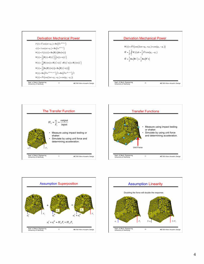
The Transfer Function
Hi1 =aiF1=outputinput
• Measure using impact testing or shaker.
• Simulate by using unit force and determining acceleration.
F1 ai
Dept. of Mech. Engineering University of Kentucky
21 ME 510 Vibro-Acoustic Design
Transfer Functions
• Measure using impact testing or shaker.
• Simulate by using unit force and determining acceleration.
Unit Force
Dept. of Mech. Engineering University of Kentucky
22
ME 510 Vibro-Acoustic Design
Assumption Superposition
F1 F2 F2
F1
+ =
aiI ai
II aiI + ai
II
aiI + ai
II = Hi1F1 +Hi2F2
Dept. of Mech. Engineering University of Kentucky
23 ME 510 Vibro-Acoustic Design
Assumption Linearity
F1 ai 2×F1 2×ai
Doubling the force will double the response.
Dept. of Mech. Engineering University of Kentucky
24
5
ME 510 Vibro-Acoustic Design
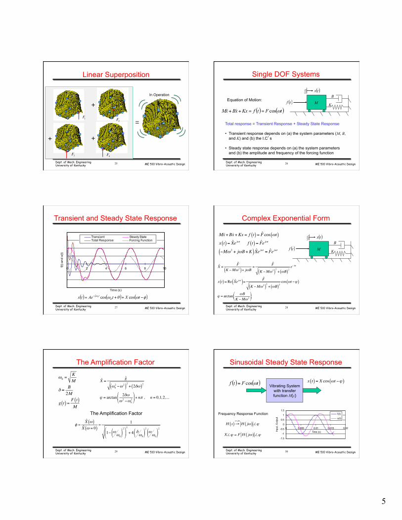
Linear Superposition
+
=
+ +
In Operation
F1 F2
F3 F4Dept. of Mech. Engineering University of Kentucky
25 ME 510 Vibro-Acoustic Design
M B
K
Total response = Transient Response + Steady State Response • Transient response depends on (a) the system parameters (M, B,
and K) and (b) the I.C’s
• Steady state response depends on (a) the system parameters and (b) the amplitude and frequency of the forcing function
Equation of Motion:
Single DOF Systems
( )tf
( )tx
( ) ( )tFtfKxxBxM ωcos==++
Dept. of Mech. Engineering University of Kentucky
26
ME 510 Vibro-Acoustic Design
0 2 4 6 8 10
Time (s)
f(t) a
nd x
(t)
Transient Steady StateTotal Response Forcing Function
( ) ( ) ( )φωθωζω −++= − tXtAetx Dtn coscos
Transient and Steady State Response
Dept. of Mech. Engineering University of Kentucky
27 ME 510 Vibro-Acoustic Design
Complex Exponential Form
M B
K ( )tf
( )txMx +Bx +Kx = f t( ) = F cos ωt( )x t( ) = Xe jωt f t( ) = Fe jωt
−Mω 2 + jωB+K( ) Xe jωt = Fe jωt
X = FK −Mω 2( )+ jωB
=F
K −Mω 2( )2+ ωB( )2
e− jϕ
x t( ) = Re Xe jωt( )= F
K −Mω 2( )2+ ωB( )2
cos ωt −ϕ( )
ϕ = arctan ωBK −Mω 2
"
#$
%
&'
Dept. of Mech. Engineering University of Kentucky
28
ME 510 Vibro-Acoustic Design Dept. of Mech. Engineering University of Kentucky
29
The Amplification Factor ω0 =
KM
δ =B2M
g t( ) =F t( )M
X = g
ω02 −ω 2( )
2+ 2δω( )2
ϕ = arctan 2δωω 2 −ω0
2
"
#$
%
&'+ nπ , n = 0,1, 2,...
φ =X ω( )
X ω = 0( )=
1
1− ωω0( )
2"
#$
%
&'
2
+ 4 δω0( )
2ωω0( )
2
The Amplification Factor
ME 510 Vibro-Acoustic Design
-1.5
-1
-0.5
0
0.5
1
1.5
0 0.005 0.01 0.015 0.02Time (s)In
put,
Out
put
f (t)
x(t)
Vibrating System with transfer function H(s)
( ) ( )tFtf ωcos= x t( ) = X cos ωt −ϕ( )
H s( )→s= jω
H jω( )∠ϕ
X∠ϕ = F H jω( )∠ϕ
Frequency Response Function
Sinusoidal Steady State Response
Dept. of Mech. Engineering University of Kentucky
30
6
ME 510 Vibro-Acoustic Design Dept. of Mech. Engineering University of Kentucky
31
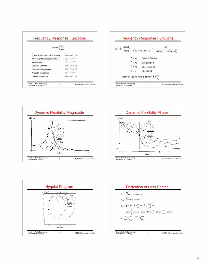
Frequency Response Functions
H ω( ) =Y ω( )X ω( )
H ω( ) = x ω( ) F ω( )Dynamic Flexibility or Receptance
Mobility or Mechanical Admittance
Accelerance
Dynamic Stiffness
Mechanical Impedance
Acoustic Impedance
Specific Impedance
H ω( ) = v ω( ) F ω( )A ω( ) = a ω( ) F ω( )
κ ω( ) = F ω( ) x ω( )
Z ω( ) = F ω( ) v ω( )
Z ω( ) = p ω( ) Q ω( )
Z ω( ) = p ω( ) u ω( )
ME 510 Vibro-Acoustic Design Dept. of Mech. Engineering University of Kentucky
32
Frequency Response Functions
H ω( ) =X ω( )F ω( )
=1
−ω 2M + jω2Mδ +K=
1 K1− ω ω0( )2 + j2 ωδ ω0
2( )
δ =ω0
δ >ω0
δ <ω0
δ = 0
Critically Damped
Overdamped
Underdamped
Undamped
ξ =δω0
Often a damping ratio is defined
ME 510 Vibro-Acoustic Design Dept. of Mech. Engineering University of Kentucky
33
Dynamic Flexibility Magnitude
ME 510 Vibro-Acoustic Design Dept. of Mech. Engineering University of Kentucky
34
Dynamic Flexibility Phase
ME 510 Vibro-Acoustic Design Dept. of Mech. Engineering University of Kentucky
35
Nyquist Diagram
ME 510 Vibro-Acoustic Design
Derivation of Loss Factor
Ekin =M2ω 2x2 cos2 ωt +ϕ( )
Epot =K2x2 sin2 ωt +ϕ( )
Edis = Fd dx∫ = B∫ dxdtdx = B∫ dx
dt"
#$
%
&'2
dt
= Bx2ω 2 cos2 ωt +ϕ( )dt0
T
∫ = Bx2ω 2 T2= Bx2ω 2 2π
2ω= Bx2ωπ
η =Edis 2πmax Epot( )
=ωBK
= 2ωδω02
Dept. of Mech. Engineering University of Kentucky
36
7
ME 510 Vibro-Acoustic Design
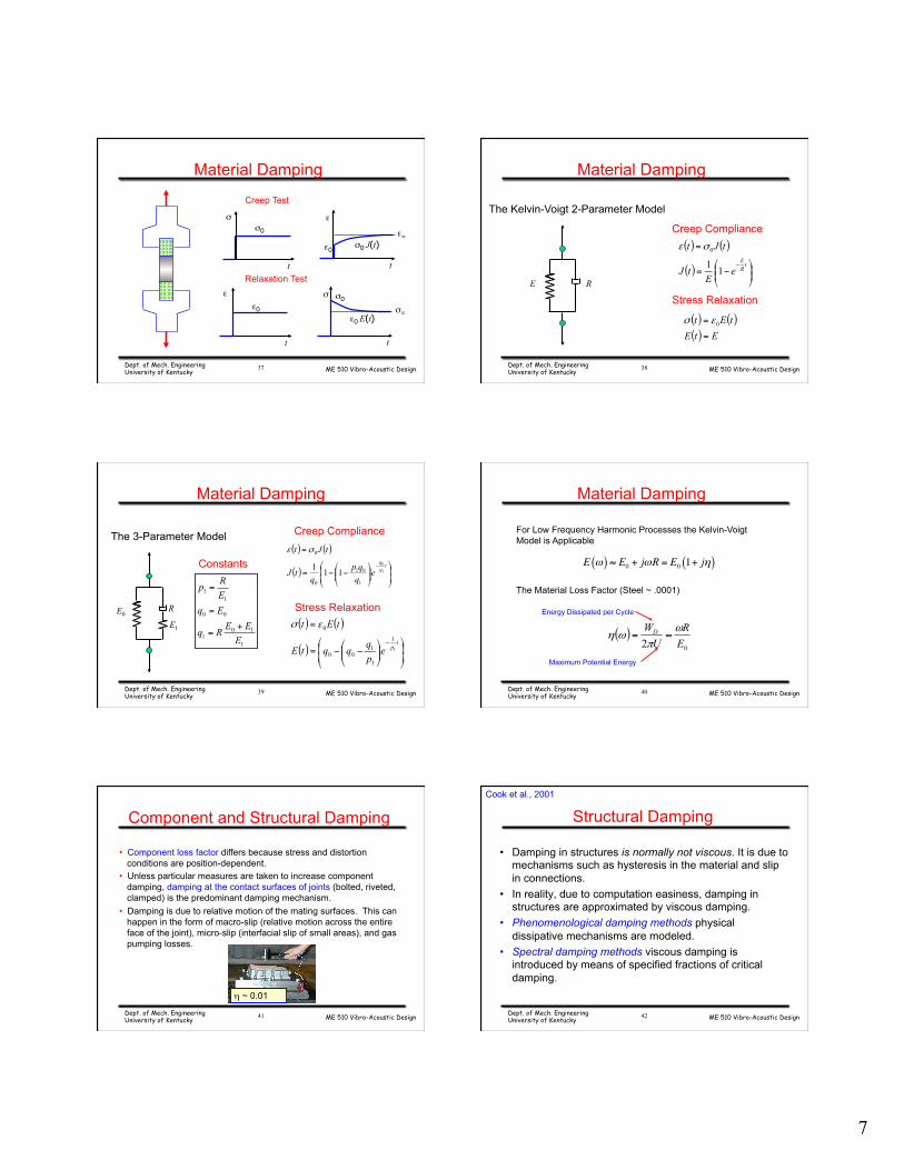
Material Damping
Creep Test
σ0 σ
t
ε0
ε
t
σ0 J(t) ε∞
Relaxation Test
ε0 ε
t
σ0 σ
t
ε0 E(t) σ∞
Dept. of Mech. Engineering University of Kentucky
37 ME 510 Vibro-Acoustic Design
The Kelvin-Voigt 2-Parameter Model
E R
Creep Compliance ( ) ( )
( ) ⎟⎟⎠
⎞⎜⎜⎝
⎛−=
=
− tRE
eE
tJ
tJt
110σε
Stress Relaxation
( ) ( )( ) EtE
tEt=
= 0εσ
Material Damping
Dept. of Mech. Engineering University of Kentucky
38
ME 510 Vibro-Acoustic Design
The 3-Parameter Model
E0 R
Creep Compliance ( ) ( )
( )⎟⎟
⎠
⎞
⎜⎜
⎝
⎛⎟⎟⎠
⎞⎜⎜⎝
⎛−−=
=
− tqq
eqqp
qtJ
tJt
1
0
1
01
0
0
111
σε
E1
Constants
1
101
00
11
EEERq
EqERp
+=
=
=
Stress Relaxation ( ) ( )
( )⎟⎟
⎠
⎞
⎜⎜
⎝
⎛⎟⎟⎠
⎞⎜⎜⎝
⎛−−=
=
− tpe
pqqqtE
tEt
1
1
1
100
0εσ
Material Damping
Dept. of Mech. Engineering University of Kentucky
39 ME 510 Vibro-Acoustic Design
For Low Frequency Harmonic Processes the Kelvin-Voigt Model is Applicable
E ω( ) ≈ E0 + jωR = E0 1+ jη( )
( )02 ER
UWD ωπ
ωη ≈=
The Material Loss Factor (Steel ~ .0001)
Energy Dissipated per Cycle
Maximum Potential Energy
Material Damping
Dept. of Mech. Engineering University of Kentucky
40
ME 510 Vibro-Acoustic Design
Component and Structural Damping
• Component loss factor differs because stress and distortion conditions are position-dependent.
• Unless particular measures are taken to increase component damping, damping at the contact surfaces of joints (bolted, riveted, clamped) is the predominant damping mechanism.
• Damping is due to relative motion of the mating surfaces. This can happen in the form of macro-slip (relative motion across the entire face of the joint), micro-slip (interfacial slip of small areas), and gas pumping losses.
η ~ 0.01
Dept. of Mech. Engineering University of Kentucky
41 ME 510 Vibro-Acoustic Design
Structural Damping
• Damping in structures is normally not viscous. It is due to mechanisms such as hysteresis in the material and slip in connections.
• In reality, due to computation easiness, damping in structures are approximated by viscous damping.
• Phenomenological damping methods physical dissipative mechanisms are modeled.
• Spectral damping methods viscous damping is introduced by means of specified fractions of critical damping.
Cook et al., 2001
Dept. of Mech. Engineering University of Kentucky
42
8
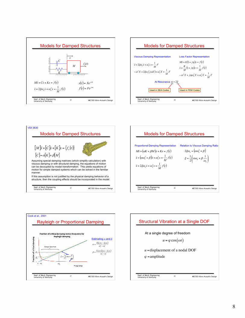
ME 510 Vibro-Acoustic Design
K
C
M fa(t)
( )
( )tfM
xxx
tfKxxCxM
nn12 2 =++
=++
ωξω
x
Models for Damped Structures
( )( ) tj
tj
FetfXetx
ω
ω
=
=
Dept. of Mech. Engineering University of Kentucky
43 ME 510 Vibro-Acoustic Design
( ) FM
XXjX
FM
xxx
nn
nn
12
12
22
2
=++−
=++
ωωξωω
ωξω
Models for Damped Structures
( ) ( )
( ) ( )
FM
XXjX
tfM
xjMKx
tfxjKxM
nn1
11
1
222 =++−
=++
=++
ωηωω
η
η
Viscous Damping Representation Loss Factor Representation
At Resonance ξη 2=
Used in SEA Codes Used in FEM Codes
Dept. of Mech. Engineering University of Kentucky
44
ME 510 Vibro-Acoustic Design
Models for Damped Structures
[ ] [ ] [ ] ( ){ }tfxKxCxM a=++
Assuming special damping matrices (which simplify calculation) with viscous damping or with structural damping, the equations of motion can be decoupled by modal transformation. This yields equations of motion for simple damped systems which can be solved in the familiar manner. If this assumption is not justified by the physical damping behavior of a structure, then the coupling effects should be incorporated in the model.
[ ] [ ] [ ]MKC βα +=
VDI 3830
Dept. of Mech. Engineering University of Kentucky
45 ME 510 Vibro-Acoustic Design
Models for Damped Structures
( ) ( )
( ) ( )
( )tfM
xxx
tfM
xxx
tfKxxMKxM
nn
nn
12
1
2
22
=++
=+++
=+++
ωξω
ωβαω
βα
( )
⎟⎟⎠
⎞⎜⎜⎝
⎛+=
+=
nn
nn
ωβαωξ
βαωξω
121
2 2
Proportional Damping Representation Relation to Viscous Damping Ratio
Dept. of Mech. Engineering University of Kentucky
46
ME 510 Vibro-Acoustic Design
Rayleigh or Proportional Damping
1ω
⎟⎠
⎞⎜⎝
⎛ +=ωβ
αωξ21
2ω
1ξ
2ξ
Design Spectrum
( )21
22
11222ωωωξωξ
α−
−=
( )21
22
1221212ωω
ωξωξωωβ
−
−=
Estimating α and β
Cook et al., 2001
Dept. of Mech. Engineering University of Kentucky
47 ME 510 Vibro-Acoustic Design
Structural Vibration at a Single DOF
At a single degree of freedom
u =ϕ cos ωt( )
u =displacement of a nodal DOFϕ =amplitude
Dept. of Mech. Engineering University of Kentucky
48
9
ME 510 Vibro-Acoustic Design
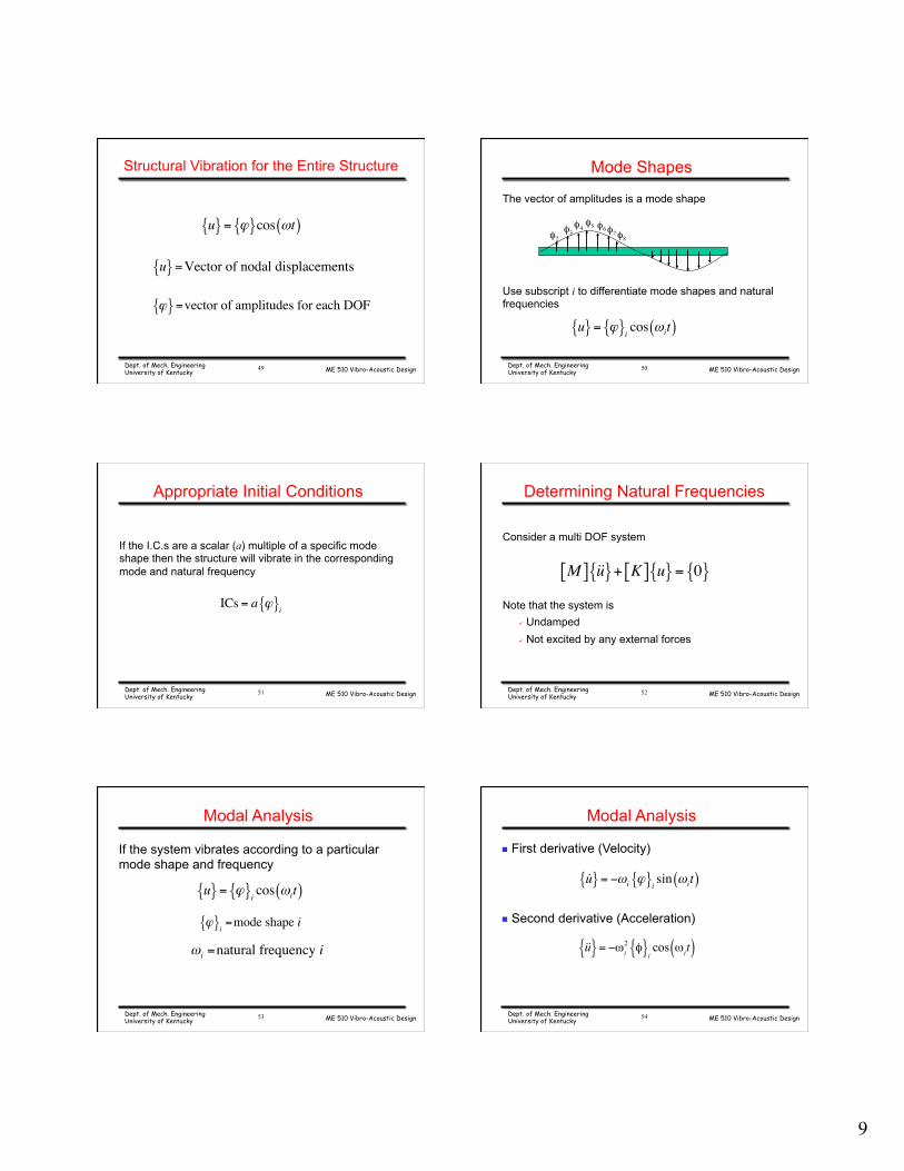
Structural Vibration for the Entire Structure
u{ }= ϕ{ }cos ωt( )
u{ }=Vector of nodal displacements
ϕ{ }=vector of amplitudes for each DOF
Dept. of Mech. Engineering University of Kentucky
49 ME 510 Vibro-Acoustic Design
Mode Shapes
The vector of amplitudes is a mode shape
2φ 3φ 4φ 5φ 6φ7φ
8φ
Use subscript i to differentiate mode shapes and natural frequencies
u{ }= ϕ{ }i cos ωit( )
Dept. of Mech. Engineering University of Kentucky
50
ME 510 Vibro-Acoustic Design
Appropriate Initial Conditions
If the I.C.s are a scalar (a) multiple of a specific mode shape then the structure will vibrate in the corresponding mode and natural frequency
ICs = a ϕ{ }i
Dept. of Mech. Engineering University of Kentucky
51 ME 510 Vibro-Acoustic Design
Determining Natural Frequencies
Consider a multi DOF system
M[ ] u{ }+ K[ ] u{ }= 0{ }
Note that the system is ü Undamped ü Not excited by any external forces
Dept. of Mech. Engineering University of Kentucky
52
ME 510 Vibro-Acoustic Design
Modal Analysis
u{ }= ϕ{ }i cos ωit( )
If the system vibrates according to a particular mode shape and frequency
ϕ{ }i =mode shape i
ωi =natural frequency i
Dept. of Mech. Engineering University of Kentucky
53 ME 510 Vibro-Acoustic Design
Modal Analysis
u{ }= −ωi ϕ{ }i sin ωit( )
g First derivative (Velocity)
g Second derivative (Acceleration)
u{ }= −ωi2 φ{ }i cos ωit( )
Dept. of Mech. Engineering University of Kentucky
54
10
ME 510 Vibro-Acoustic Design
Modal Analysis
− M"# $%ωi2 + K"# $%( ) φ{ }i = 0{ }
Plug velocity and acceleration into the equation of motion
Two possible solutions
φ{ }i = 0{ }
det − M"# $%ωi2 + K"# $%( ) = 0
Dept. of Mech. Engineering University of Kentucky
55 ME 510 Vibro-Acoustic Design
The Eigen Problem
The Eigen Problem
A!" #$ x{ }= λ x{ }
det − M"# $%ωi2 + K"# $%( ) = 0
λEigenvalue
x{ }Eigenvector
Dept. of Mech. Engineering University of Kentucky
56
ME 510 Vibro-Acoustic Design
Modal Analysis – An Eigen Problem
− M"# $%ωi2 + K"# $%( ) φ{ }= 0"# $%
Natural frequencies are eigenvalues
The mode shapes are eigenvectors
K!" #$ φ{ }=ωi2 M!" #$ φ{ }
M!" #$−1K!" #$ φ{ }=ωi2 φ{ }
ωi2
φ{ }Dept. of Mech. Engineering University of Kentucky
57 ME 510 Vibro-Acoustic Design
Modal Analysis – An Eigen Problem
Solving the eigen problem
M!" #$−1K!" #$ φ{ }=ωi2 φ{ }
A!" #$ x{ }= λ x{ }
A!" #$ x{ }−λ x{ }= 0A!" #$− λ I!" #$( ) x{ }= 0det A!" #$− λ I!" #$( ) = 0
Dept. of Mech. Engineering University of Kentucky
58
ME 510 Vibro-Acoustic Design
Example Eigen Problem
2 33 2
!
"#
$
%&x1x2
!"#
$#
%&#
'#= λi
x1x2
!"#
$#
%&#
'#
det 2 33 2
(
)*
+
,-− λi
1 00 1
!
"#
$
%&
'
())
*
+,,= 0
Dept. of Mech. Engineering University of Kentucky
59 ME 510 Vibro-Acoustic Design
Find Eigenvalues
det 2−λ 33 2−λ
#
$%
&
'(
)
*++
,
-..= 0
2−λ( ) 2−λ( )−9 = λ2 − 4λ −5Eigen values
λ1 = −1λ2 = 5
Dept. of Mech. Engineering University of Kentucky
60
11
ME 510 Vibro-Acoustic Design
For Eigen Vector 1
λ1 = −1
2 33 2
#
$%
&
'(− −1( ) 1 0
0 1
#
$%
&
'(
)
*++
,
-..
x1x2
/01
21
341
511
= 00
/01
21
341
51
2+1 33 2+1
#
$%
&
'(
)
*++
,
-..
x1x2
/01
21
341
511
= 00
/01
21
341
51
Dept. of Mech. Engineering University of Kentucky
61 ME 510 Vibro-Acoustic Design
For Eigen Vector 1
3 33 3
!
"#
$
%&
'
())
*
+,,
x1x2
-./
0/
12/
3/1
= 00
-./
0/
12/
3/
x1 can be any value
x1x2
!"#
$#
%&#
'#1
= 1−1
!"#
$#
%&#
'#= .7071
−.7071
!"#
$#
%&#
'#
Dept. of Mech. Engineering University of Kentucky
62
ME 510 Vibro-Acoustic Design
For Eigen Vector 2
λ2 = 5
2 33 2
"
#$
%
&'− 5( ) 1 0
0 1
"
#$
%
&'
)
*++
,
-..
x1x2
/01
21
341
512
= 00
/01
21
341
51
2−5 33 2−5
"
#$
%
&'
)
*++
,
-..
x1x2
/01
21
341
512
= 00
/01
21
341
51
Dept. of Mech. Engineering University of Kentucky
63 ME 510 Vibro-Acoustic Design
For Eigen Vector 2
−3 33 −3
"
#$
%
&'
(
)**
+
,--
x1x2
./0
10
230
402
= 00
./0
10
230
40
x2 = x1
x2 can be any value
x1x2
!"#
$#
%&#
'#2
= 11
!"#
$#
%&#
'#= .7071
.7071
!"#
$#
%&#
'#
Dept. of Mech. Engineering University of Kentucky
64
ME 510 Vibro-Acoustic Design
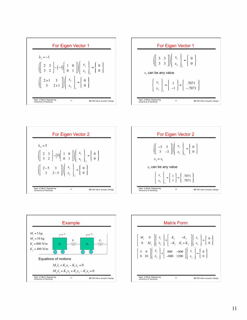
Example
Equations of motions
M1 M2 K1 K2
x1 x2
M1x1 + K1x1 − K1x2 = 0M 2x2 + K2x2 + K1x2 − K1x1 = 0
M1 = 5 kgM 2 =10 kgK1 = 800 N/mK2 = 400 N/m
Dept. of Mech. Engineering University of Kentucky
65 ME 510 Vibro-Acoustic Design
Matrix Form
M1 0
0 M 2
!
"
##
$
%
&&
x1x2
'()
*)
+,)
-)+
K1 −K1−K1 K1 + K2
!
"
##
$
%
&&
x1x2
'()
*)
+,)
-)= 0
0
'()
*)
+,)
-)
5 00 10
!
"#
$
%&x1x2
'()
*)
+,)
-)+ 800 −800
−800 1200
!
"#
$
%&x1x2
'()
*)
+,)
-)= 0
0
'()
*)
+,)
-)
Dept. of Mech. Engineering University of Kentucky
66
12
ME 510 Vibro-Acoustic Design
Set Up Eigen Problem
M!" #$−1K!" #$ φ{ }=ωi2 φ{ }
M!" #$−1K!" #$=
160 −160−80 120
!
"(
#
$)
det 160 −160−80 120
!
"(
#
$)− λ 1 0
0 1
!
"(
#
$)
+
,--
.
/00= 0
Dept. of Mech. Engineering University of Kentucky
67 ME 510 Vibro-Acoustic Design
Solve Eigen Problem
det 160−λ −160−80 120−λ
#
$%
&
'(
)
*++
,
-..= 0
ω1 = λ1 = 5.011 rad/s
f1 =5.011
2π= .7975 Hz
ω2 = λ2 =15.965 rad/s
f2 =15.965
2π= 2.5409 Hz
φ1φ2
"#$
%$
&'$
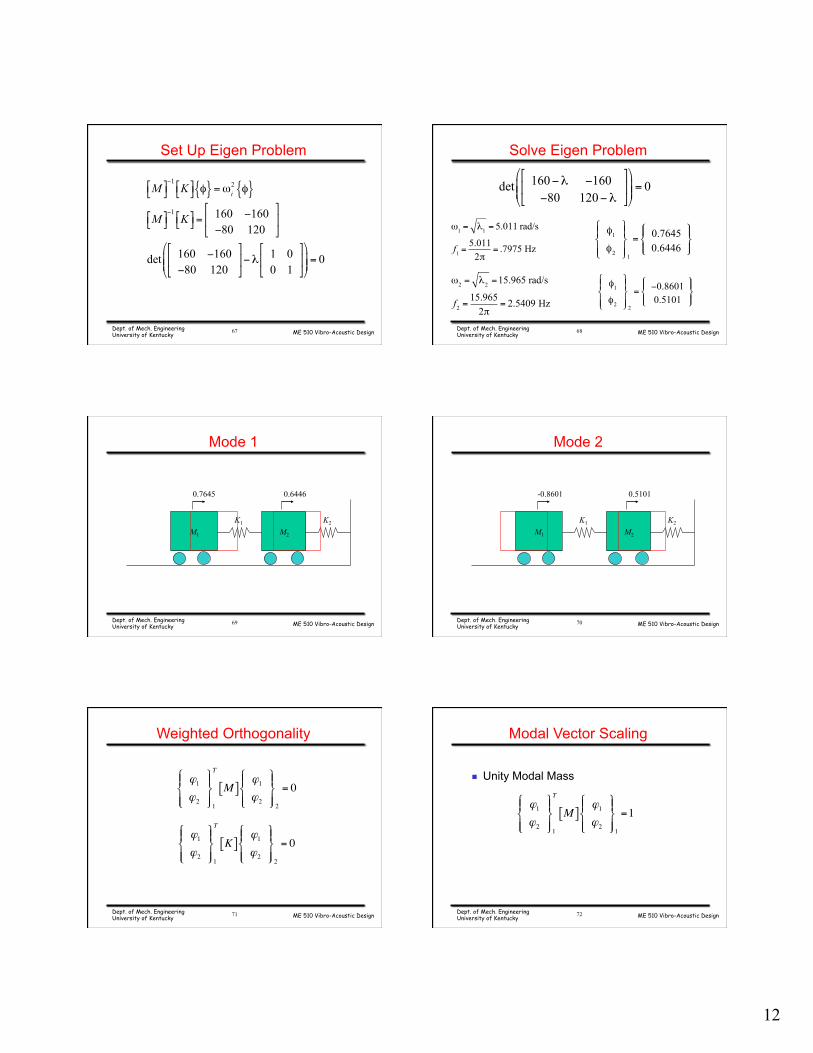
($1
= 0.76450.6446
"#$
%$
&'$
($
φ1φ2
"#$
%$
&'$
($2
= −0.86010.5101
"#$
%$
&'$
($
Dept. of Mech. Engineering University of Kentucky
68
ME 510 Vibro-Acoustic Design
Mode 1
M1 M2 K1 K2
0.7645 0.6446
Dept. of Mech. Engineering University of Kentucky
69 ME 510 Vibro-Acoustic Design
Mode 2
M1 M2 K1 K2
-0.8601 0.5101
Dept. of Mech. Engineering University of Kentucky
70
ME 510 Vibro-Acoustic Design
Weighted Orthogonality
ϕ1ϕ2
!"#
$#
%&#
'#1
T
M[ ]ϕ1ϕ2
!"#
$#
%&#
'#2
= 0
ϕ1ϕ2
!"#
$#
%&#
'#1
T
K[ ]ϕ1ϕ2
!"#
$#
%&#
'#2
= 0
Dept. of Mech. Engineering University of Kentucky
71 ME 510 Vibro-Acoustic Design
Modal Vector Scaling
ϕ1ϕ2
!"#
$#
%&#
'#1
T
M[ ]ϕ1ϕ2
!"#
$#
%&#
'#1
=1
g Unity Modal Mass
Dept. of Mech. Engineering University of Kentucky
72
13
ME 510 Vibro-Acoustic Design
Modal Vector Scaling
.7645X
.6446X
!"#
$%&1
T5 00 10
'
()
*
+,.7645X.6446X
!"#
$%&1=1
g Unity Modal Mass
X = .376
ϕ1ϕ2
!"#
$#
%&#
'#1
= .287.242
!"$
%&'
Dept. of Mech. Engineering University of Kentucky
73 ME 510 Vibro-Acoustic Design
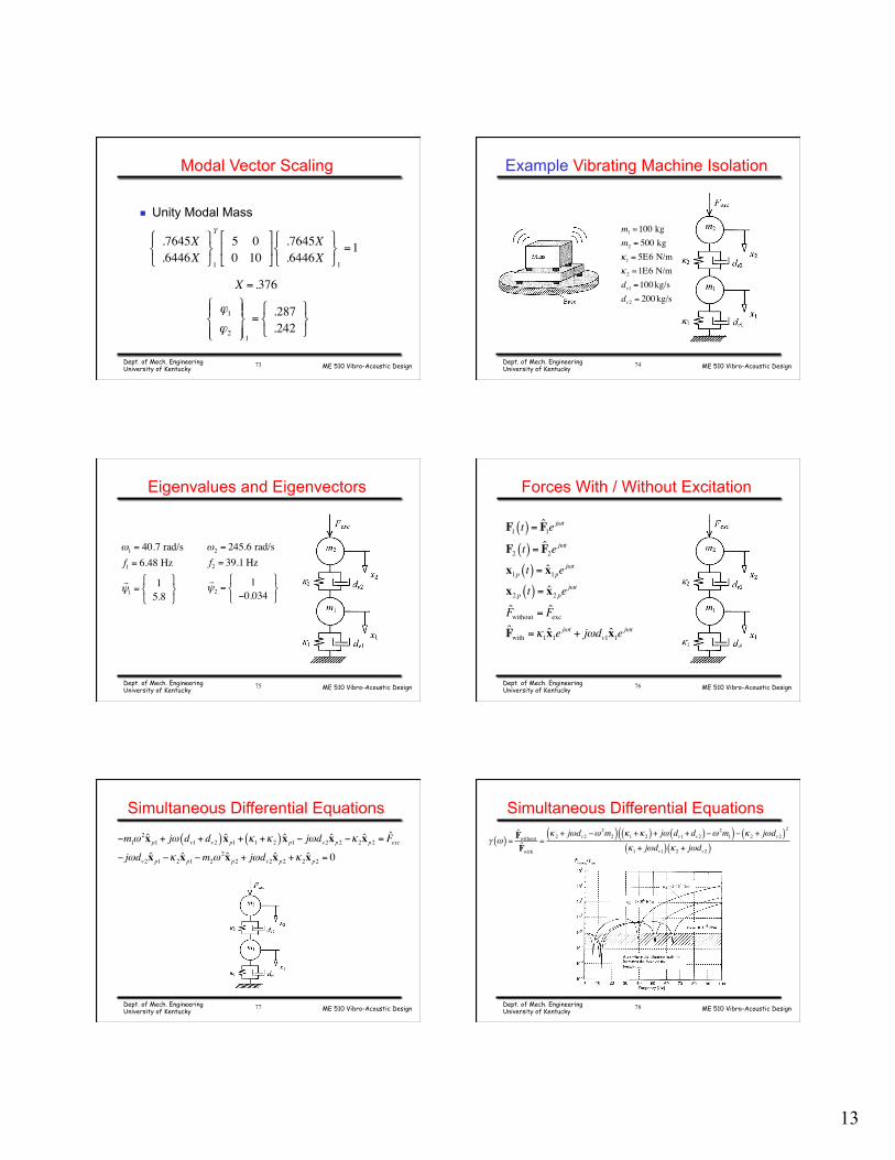
Example Vibrating Machine Isolation
m1 =100 kgm2 = 500 kgκ1 = 5E6 N/mκ2 =1E6 N/mdv1 =100kg/sdv2 = 200kg/s
Dept. of Mech. Engineering University of Kentucky
74
ME 510 Vibro-Acoustic Design
Eigenvalues and Eigenvectors
ω1 = 40.7 rad/sf1 = 6.48 Hzψ1 =
15.8
!"#
$%&
ω2 = 245.6 rad/sf2 = 39.1 Hzψ2 =
1−0.034
"#$
%&'
Dept. of Mech. Engineering University of Kentucky
75 ME 510 Vibro-Acoustic Design
Forces With / Without Excitation
F1 t( ) = F1e jωt
F2 t( ) = F2e jωt
x1p t( ) = x1pe jωt
x2 p t( ) = x2 pe jωt
Fwithout = FexcFwith =κ1x1e
jωt + jωdv1x1ejωt
Dept. of Mech. Engineering University of Kentucky
76
ME 510 Vibro-Acoustic Design
Simultaneous Differential Equations
−m1ω2x p1 + jω dv1 + dv2( ) x p1 + κ1 +κ2( ) x p1 − jωdv2x p2 −κ2x p2 = Fexc
− jωdv2x p1 −κ2x p1 −m2ω2x p2 + jωdv2x p2 +κ2x p2 = 0
Dept. of Mech. Engineering University of Kentucky
77 ME 510 Vibro-Acoustic Design
Simultaneous Differential Equations
γ ω( ) = FwithoutFwith
=κ2 + jωdv2 −ω
2m2( ) κ1 +κ2( )+ jω dv1 + dv2( )−ω 2m1( )− κ2 + jωdv2( )2
κ1 + jωdv1( ) κ2 + jωdv2( )
Dept. of Mech. Engineering University of Kentucky
78
14
ME 510 Vibro-Acoustic Design
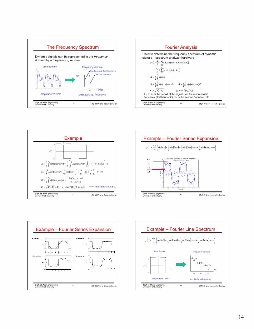
The Frequency Spectrum
Dynamic signals can be represented in the frequency domain by a frequency spectrum
f (Hz)
10
1 2
amplitude vs. time
time domain frequency domain
amplitude vs. frequency
Fundamental (first harmonic)
Second harmonic
Dept. of Mech. Engineering University of Kentucky
79 ME 510 Vibro-Acoustic Design
Fourier Analysis Used to determine the frequency spectrum of dynamic signals – spectrum analyzer hardware
T = 2π/ω Is the period of the signal, ω is the fundamental frequency (first harmonic), 2ω is the second harmonic, etc.
y t( ) = Ao2+ An cos nωt( )+Bn sin nωt( )( )
n=1
∞
∑
=Ao2+ Cn cos nωt −ϕn( )( )
n=1
∞
∑
A0 =2T
y t( )dt0
T
∫
An =2T
y t( )cos nωt( )dt0
T
∫ Bn =2T
y t( )sin nωt( )dt0
T
∫
Cn = An2 +Bn
2 ϕn = tan−1 Bn An( )
Dept. of Mech. Engineering University of Kentucky
80
ME 510 Vibro-Acoustic Design
Example
t
A
-A
T
y(t)
Phase between An & Bn
An =2T
y t( )0
T
∫ cos nωt( )dt = 2T
Acos nωt( )dt +0
T 2
∫ −A( )cos nωt( )dtT 2
T
∫#
$%%
&
'((= 0
i.e., Acos nωt( )dt0
T 2
∫ =Anωsin nωt( )
0
T 2
=Anω
sin n 2πTT2
)
*+
,
-.− 0
#
$%
&
'(= 0
Bn =2T
y t( )0
T
∫ sin nωt( )dt =4A nπ , n odd0, n even
/01
21
Cn = An2 +Bn
2 = Bn ϕn = tan−1 Bn An( ) = π 2
Dept. of Mech. Engineering University of Kentucky
81 ME 510 Vibro-Acoustic Design
Example – Fourier Series Expansion
( ) ( ) ( ) ( ) ( ) ⎟⎠
⎞⎜⎝
⎛ +++++= tnn
tttAty ωωωωπ
sin15sin513sin
31sin4
πA4
π34A
Dept. of Mech. Engineering University of Kentucky
82
ME 510 Vibro-Acoustic Design
Example – Fourier Series Expansion
Dept. of Mech. Engineering University of Kentucky
83 ME 510 Vibro-Acoustic Design
amplitude vs. time
time domain
t
A
-A
T
y(t)
ω 3ω
frequency domain
amplitude vs.frequency
5ω
etc.
Example – Fourier Line Spectrum
( ) ( ) ( ) ( ) ( ) ⎟⎠
⎞⎜⎝
⎛ +++++= tnn
tttAty ωωωωπ
sin15sin513sin
31sin4
πA4
π34Aπ54A
Dept. of Mech. Engineering University of Kentucky
84
15
ME 510 Vibro-Acoustic Design
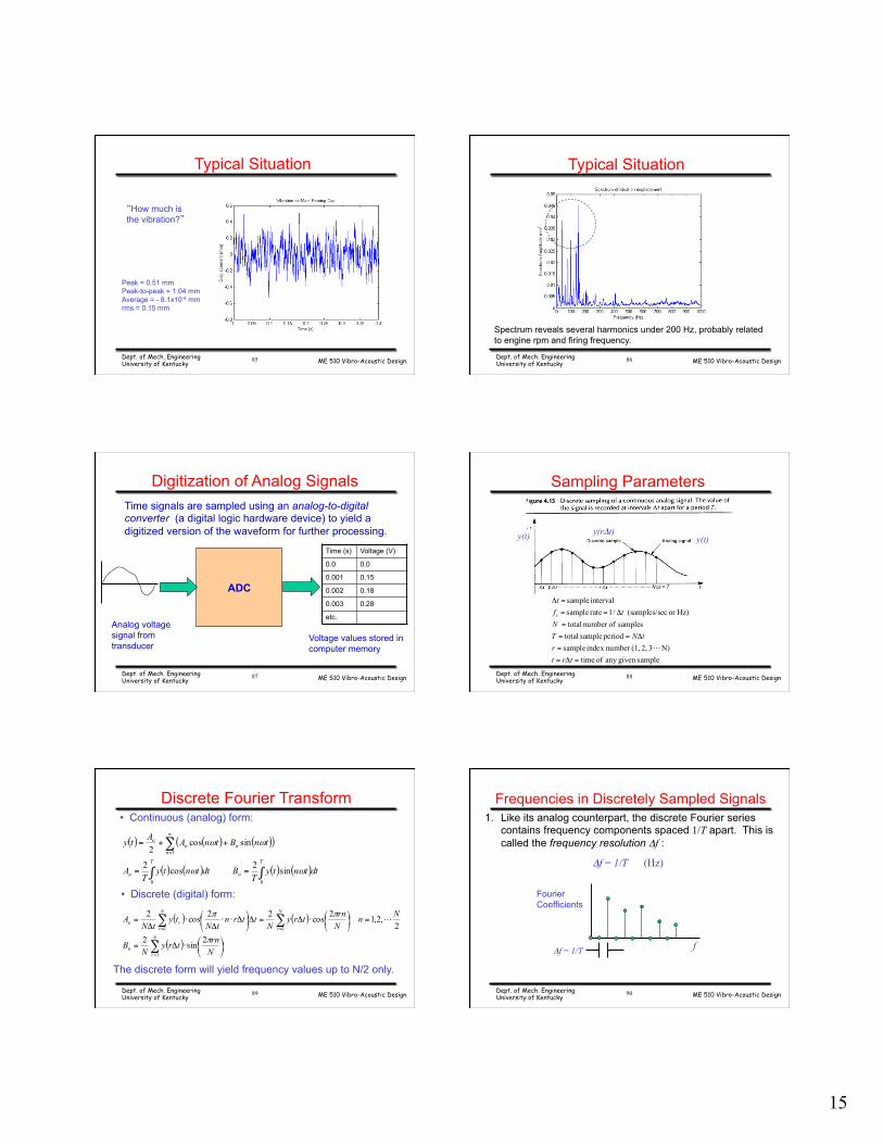
“How much is the vibration?”
Peak = 0.51 mm Peak-to-peak = 1.04 mm Average = - 8.1x10⁻⁴ mm rms = 0.15 mm
Typical Situation
Dept. of Mech. Engineering University of Kentucky
85 ME 510 Vibro-Acoustic Design
Spectrum reveals several harmonics under 200 Hz, probably related to engine rpm and firing frequency.
Typical Situation
Dept. of Mech. Engineering University of Kentucky
86
ME 510 Vibro-Acoustic Design
Digitization of Analog Signals Time signals are sampled using an analog-to-digital converter (a digital logic hardware device) to yield a digitized version of the waveform for further processing.
ADC
Analog voltage signal from transducer
Time (s) Voltage (V)
0.0 0.0
0.001 0.15
0.002 0.18
0.003 0.28
etc.
Voltage values stored in computer memory
Dept. of Mech. Engineering University of Kentucky
87 ME 510 Vibro-Acoustic Design
samplegiven any of timeN)3 2, (1,number index sample
period sample totalsamples ofnumber total
Hz)or ec(samples/s /1 rate sample interval sample
=Δ=
⋅⋅⋅=
Δ==
=
Δ==
=Δ
trtr
tNTN
tft
s
Sampling Parameters
y(t) y(rΔt) y(t)
Dept. of Mech. Engineering University of Kentucky
88
ME 510 Vibro-Acoustic Design
Discrete Fourier Transform • Continuous (analog) form:
• Discrete (digital) form:
The discrete form will yield frequency values up to N/2 only.
( ) ( ) ( )( )
( ) ( ) ( ) ( )∫∫
∑
==
++=∞
=
T
n
T
n
nnn
o
dttntyT
BdttntyT
A
tnBtnAAty
00
1
sin2cos2
sincos2
ωω
ωω
( ) ( )
( ) ⎟⎠
⎞⎜⎝
⎛⋅Δ=
=⎟⎠
⎞⎜⎝
⎛⋅Δ=Δ⎟⎠
⎞⎜⎝
⎛ Δ⋅⋅Δ
⋅Δ
=
∑
∑∑
=
==
Nrntry
NB
NnNrntry
Nttrn
tNty
tNA
N
rn
N
r
N
rrn
π
ππ
2sin22
,2,12cos22cos2
1
11
Dept. of Mech. Engineering University of Kentucky
89 ME 510 Vibro-Acoustic Design
Frequencies in Discretely Sampled Signals 1. Like its analog counterpart, the discrete Fourier series
contains frequency components spaced 1/T apart. This is called the frequency resolution Δf :
Δf = 1/T (Hz)
Δf = 1/T f
Fourier Coefficients
Dept. of Mech. Engineering University of Kentucky
90
16
ME 510 Vibro-Acoustic Design
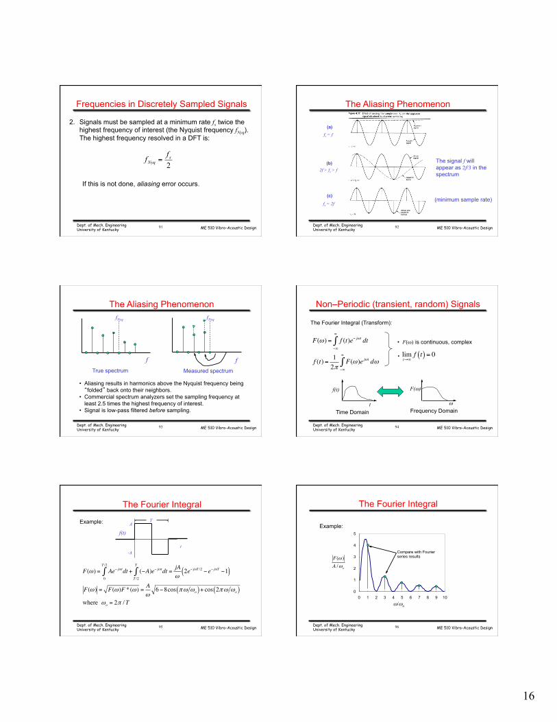
Frequencies in Discretely Sampled Signals
2s
Nyqff =
2. Signals must be sampled at a minimum rate fs twice the highest frequency of interest (the Nyquist frequency fNyq). The highest frequency resolved in a DFT is:
If this is not done, aliasing error occurs.
Dept. of Mech. Engineering University of Kentucky
91 ME 510 Vibro-Acoustic Design
The Aliasing Phenomenon
fs = f
(a)
(b)
(c)
2f > fs > f
fs = 2f (minimum sample rate)
The signal f will appear as 2f/3 in the spectrum
Dept. of Mech. Engineering University of Kentucky
92
ME 510 Vibro-Acoustic Design
The Aliasing Phenomenon
True spectrum
fNyq
f Measured spectrum
fNyq
f
• Aliasing results in harmonics above the Nyquist frequency being “folded” back onto their neighbors.
• Commercial spectrum analyzers set the sampling frequency at least 2.5 times the highest frequency of interest.
• Signal is low-pass filtered before sampling.
Dept. of Mech. Engineering University of Kentucky
93 ME 510 Vibro-Acoustic Design Dept. of Mech. Engineering University of Kentucky
Non–Periodic (transient, random) Signals
The Fourier Integral (Transform):
F(ω) = f (t)e− jωt dt−∞
∞
∫
f (t) = 12π
F(ω)e jωt dω−∞
∞
∫
t
f(t)
ω
F(ω)
Time Domain Frequency Domain
• F(ω) is continuous, complex
• limt→∞f t( ) = 0
94
ME 510 Vibro-Acoustic Design Dept. of Mech. Engineering University of Kentucky
The Fourier Integral
Example:
t
A
-A
T
f(t)
F(ω) = Ae− jωt0
T /2
∫ dt + (−A)e− jωtT /2
T
∫ dt = jAω
2e− jωT /2 − e− jωT −1( )
F(ω) = F(ω)F *(ω) = Aω
6−8cos πω ωo( )+ cos 2πω ωo( )
where ωo = 2π /T
95 ME 510 Vibro-Acoustic Design Dept. of Mech. Engineering University of Kentucky
The Fourier Integral
Example:
0
1
2
3
4
5
0 1 2 3 4 5 6 7 8 9 10
ω/ωo
F(ω)A /ωo
Compare with Fourier series results
96
17
ME 510 Vibro-Acoustic Design Dept. of Mech. Engineering University of Kentucky
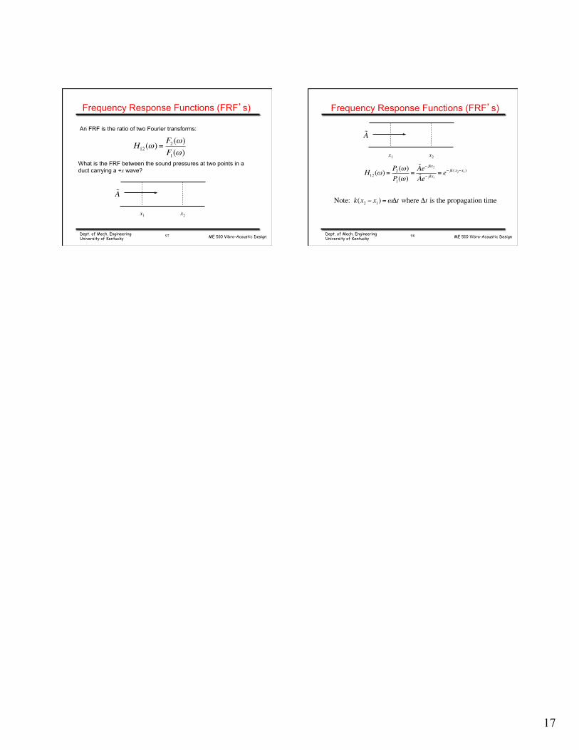
Frequency Response Functions (FRF’s)
An FRF is the ratio of two Fourier transforms:
H12 (ω) =F2 (ω)F1(ω)
What is the FRF between the sound pressures at two points in a duct carrying a +x wave?
A
x1 x2
97 ME 510 Vibro-Acoustic Design Dept. of Mech. Engineering University of Kentucky
Frequency Response Functions (FRF’s)
H12 (ω) = P2 (ω)P1(ω)
=Ae− jkx2
Ae− jkx1= e− jk (x2−x1 )
Note: k(x2 − x1) =ωΔt where Δt is the propagation time
A
x1 x2
98


![Arkfn[mathematical methods for physicsists]](https://static.fdocument.org/doc/165x107/554a2400b4c90542548b483a/arkfnmathematical-methods-for-physicsists.jpg)