arX

iv:h

ep-p

h/00

0421

3v3

8 N

ov 2

000

Branching Ratio and CP Violation of B → ππ Decays

in Perturbative QCD Approach

Cai-Dian Lua∗, Kazumasa Ukaib†, Mao-Zhi Yanga‡

a Physics Department, Hiroshima University, Higashi-Hiroshima 739-8526, Japan

b Physics Department, Nagoya University, Nagoya 464-8602, Japan

October 31, 2018

hep-ph/0004213

HUPD-9924

DPNU-00-15

Abstract

We calculate the branching ratios and CP asymmetries for B0 → π+π−, B+ → π

+π0

and B0 → π0π0 decays, in a perturbative QCD approach. In this approach, we calculate

non-factorizable and annihilation type contributions, in addition to the usual factorizable

contributions. We found that the annihilation diagram contributions are not very small

as previous argument. Our result is in agreement with the measured branching ratio of

B → π+π− by CLEO collaboration. With a non-negligible contribution from annihilation

diagrams and a large strong phase, we predict a large direct CP asymmetry inB0 → π

+π−,

and π0π0, which can be tested by the current running B factories.

PACS: 13.25.Hw, 11,10.Hi, 12,38.Bx,

∗e-mail: lucd@theo.phys.sci.hiroshima-u.ac.jp†e-mail: ukai@eken.phys.nagoya-u.ac.jp‡e-mail: yangmz@theo.phys.sci.hiroshima-u.ac.jp

1

1 Introduction

The charmless B decays arouse more and more interests recently, since it is a good place

for study of CP violation and it is also sensitive to new physics [1]. Factorization approach

(FA) is applied to hadronic B decays and is generalized to decay modes that are classified

in the spin of final states [2, 3, 4]. FA gives predictions in terms of form factors and decay

constants. Although the predictions of branching ratios agree well with experiments in most

cases, there are still some theoretical points unclear. First, it relies strongly on the form

factors, which cannot be calculated by FA itself. Secondly, the generalized FA shows that the

non-factorizable contributions are important in a group of channels [3, 4]. The reason of this

large non-factorizable contribution needs more theoretical studies. Thirdly, the strong phase,

which is important for the CP violation prediction, is quite sensitive to the internal gluon

momentum [5]. This gluon momentum is the sum of momenta of two quarks, which go into two

different mesons. It is difficult to define exactly in the FA approach. To improve the theoretical

predictions of the non-leptonic B decays, we try to improve the factorization approach, and

explain the size of the non-factorizable contributions in a new approach.

We shall take a specific channel B → ππ as an example. The B → ππ decays are responsible

for the determination of the angle φ2 in the unitarity triangle which have been studied in the

factorization approach in detail [2, 3, 4]. The recent measurements of B → π+π− by CLEO

Collaboration attracted much attention for these kind of decays [6]. The most recent theoretical

study [7] attempted to compute the non-factorizable diagrams directly. But it could not also

predict the transition form factors of B → π.

In this paper, we would like to study the B → ππ decays in the perturbative QCD approach

(PQCD) [8]. In the B → ππ decays, the B meson is heavy, sitting at rest. It decays into two

light mesons with large momenta. Therefore the light mesons are moving very fast in the rest

frame of B meson. In this case, the short distance hard process dominates the decay amplitude.

We shall demonstrate that the soft final state interaction is not important, since there is not

enough time for the pions to exchange soft gluons. This makes the perturbative QCD approach

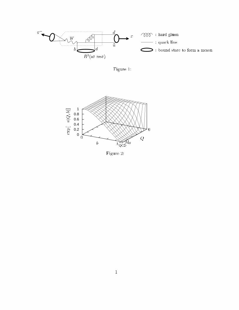
applicable. With the final pions moving very fast, there must be a hard gluon to kick the light

spectator quark d or u (almost at rest) in the B meson to form a fast moving pion (see Figure 1).

So the dominant diagram in this theoretical picture is that one hard gluon from the spectator

2

quark connecting with the other quarks in the four quark operator of the weak interaction.

Unlike the usual FA, where the spectator quark does not participate in the decay process in a

major way, the hard part of the PQCD approach consists of six quarks rather than four. We

thus call it six-quark operators or six-quark effective theory. Applying the six-quark effective

theory to B meson exclusive decays, we need meson wave functions for the hadronization of

quarks into mesons. Separating that nonperturbative dynamics from the hard one, the decay

amplitudes can be calculated in PQCD easily. Most of the nonperturbative dynamics are

included in the meson wave functions, but in the correction that soft gluon straddle the six-

quark operators, there are some nonfactorizable soft gluon effects not to be absorbed into the

meson wave functions. Such effects can be safely neglected in the B meson decays [9].

Li performed the calculation of B0 → π+π− in ref.[10] using the PQCD formalism, where the

factorizable tree diagrams were calculated and the branching ratios were predicted. In another

paper [11], Dahm, Jakob and Kroll performed a more complete calculation, including the non-

factorizable annihilation topology and the three decay channels ofB → ππ decays. However, the

predicted branching ratios are about one order smaller than the current experiments by CLEO

[6]. In connection with this, Feldmann and Kroll concluded that perturbative contributions to

the B → π transition form factor were much smaller than nonperturbative ones [12]. As we

shall show later, the pion wave function must be consistent with chiral symmetry relation

− qµ〈0|uγµγ5d(x)|π−(q)〉 = (mu +md)〈0|uγ5d(x)|π−(q)〉. (1)

This introduces terms that were not considered in above calculations. In this paper, considering

the terms needed from chiral symmetry, we calculate the B → π transition form factors and

also the non-factorizable contributions in PQCD approach. We then show that our result for

the branching ratio B → π+π− agree with the measurement. Among the new terms, it is

worthwhile emphasizing the presence of annihilation diagrams which are ignored in FA. We

find that these diagrams can not be ignored, and furthermore they contribute to large final

state interaction phase.

3

2 The Frame Work

The three scale PQCD factorization theorem has been developed for non-leptonic heavy meson

decays [13], based on the formalism by Brodsky and Lepage [14], and Botts and Sterman [15].

The QCD corrections to the four quark operators are usually summed by the renormalization

group equation [16]. This has already been done to the leading logarithm and next-to-leading

order for years. Since the b quark decay scalemb is much smaller than the electroweak scalemW ,

the QCD corrections are non-negligible. The third scale 1/b involved in the B meson exclusive

decays is usually called the factorization scale, with b the conjugate variable of parton transverse

momenta. The dynamics below 1/b scale is regarded as being completely nonperturbative, and

can be parametrized into meson wave functions. The meson wave functions are not calculable

in PQCD. But they are universal, channel independent. We can determine it from experiments,

and it is constrained by QCD sum rules and Lattice QCD calculations. Above the scale 1/b, the

physics is channel dependent. We can use perturbation theory to calculate channel by channel.

Besides the hard gluon exchange with the spectator quark, the soft gluon exchanges between

quark lines give out the double logarithms ln2(Pb) from the overlap of collinear and soft diver-

gences, P being the dominant light-cone component of a meson momentum. The resummation

of these double logarithms leads to a Sudakov form factor exp[−s(P, b)], which suppresses the

long distance contributions in the large b region, and vanishes as b > 1/ΛQCD. This form factor

is given to sum the leading order soft gluon exchanges between the hard part and the wave

functions of mesons. So this term includes the double infrared logarithms. The expression of

s(Q, b) is concretely given in appendix B. Figure 2 shows that e−s falls off quickly in the large b,

or long-distance, region, giving so-called Sudakov suppression. This Sudakov factor practically

makes PQCD approach applicable. For the detailed derivation of the Sudakov form factors, see

ref.[8, 17].

With all the large logarithms resummed, the remaining finite contributions are absorbed

into a perturbative b quark decay subamplitude H(t). Therefore the three scale factorization

formula is given by the typical expression,

C(t)×H(t)× Φ(x)× exp

[

−s(P, b)− 2∫ t

1/b

dµ

µγq(αs(µ))

]

, (2)

where C(t) are the corresponding Wilson coefficients, Φ(x) are the meson wave functions and

4

the variable t denotes the largest mass scale of hard process H , that is, six-quark effective

theory. The quark anomalous dimension γq = −αs/π describes the evolution from scale t to

1/b. Since logarithm corrections have been summed by renormalization group equations, the

above factorization formula does not depend on the renormalization scale µ explicitly.

The three scale factorization theorem in eq.(2) is discussed by Li et al. in detail [13]. Below

section 3, we shall give the factorization formulae for B → ππ decay amplitudes by calculating

the hard part H(t), channel dependent in PQCD. We shall also approximate H there by the

O(αs) expression, which makes sense if perturbative contributions indeed dominate.

In the resummation procedures, the B meson is treated as a heavy-light system. The wave

function is defined as

ΦB =1√2Nc

( 6pB +mB)γ5φB(k1, kb), (3)

where Nc = 3 is color’s degree of freedom and φB(k1, kb) is the distribution function of the

4-momenta of the light quark (k1) and b quark (kb)

φB(k1, kb) =1

p2B

1

2√2Nc

∫

d4y

(2π)4eik1·y〈0|T[d(y) 6pBγ5b(0)]|B(pB)〉. (4)

Note that we use the same distribution function φB(k1, kb) for the 6 pB term and the mB term

from heavy quark effective theory. For the hard part calculations in the next section, we use

the approximation mb ≃ mB, which is the same order approximation neglecting higher twist

of (mB −mb)/mB. To form a bound state of B meson, the condition kb = pB − k1 is required.

So φB is actually a function of k1 only. Through out this paper, we take p± = (p0 ± p3)/√2,

pT = (p1, p2) as the light-cone coordinates to write the four momentum. We consider the B

meson at rest, then that momentum is pB = (mB/√2)(1, 1, 0T ). The momentum of the light

valence quark is written as (k+1 , k

−1 ,k1T ), where the k1T is a small transverse momentum. It is

difficult to define the function φB(k+1 , k

−1 ,k1T ). However, in the next section, we will see that

the hard part is always independent of k+1 , if we make some approximations. This means that

k+1 can be integrated out in eq.(4), the function φB(k

+1 , k

−1 ,k1T ) can be simplified to

φB(x1,k1T ) = p−B

∫

dk+1 φB(k

+1 , k

−1 ,k1T )

=p−Bp2B

1

2√2Nc

∫

dy+d2yT

(2π)3ei(k

−

1y+−k1T ·yT )〈0|T[d(y+, 0,yT ) 6pBγ5b(0)]|B(pB)〉, (5)

where x1 = k−1 /p

−B is the momentum fraction. Therefore, in the perturbative calculations, we

5

do not need the information of all four momentum k1. The above integration can be done only

when the hard part of the subprocess is independent of the variable k+1 .

The π meson is treated as a light-light system. At the B meson rest frame, pion is moving

very fast. We define the momentum of the pion which contain the spectator light quark as

P2 = (mB/√2)(1, 0, 0T ). The other pion which moving to the inverse direction, then has

momentum P3 = (mB/√2)(0, 1, 0T ). The light spectator quark moving with the pion (with

momentum P2), has a momentum (k+2 , 0,k2T ). The momentum of the other valence quark in

this pion is then (P+2 − k+

2 , 0,−k2T ). If we define the momentum fraction as x2 = k+2 /P

+2 , then

the wave function of pion can be written as

Φπ =1√2Nc

γ5 [6pπφπ(x2,k2T ) +m0φ′π(x2,k2T )] , (6)

where φπ(x2,k2T ) is defined in analogue to eq.(4, 5) and φ′π(x2,k2T ) is defined by

φ′π(x2,k2T ) =

P+2

2√2Nc

∫

dy−d2yT

(2π)3ei(x2P

+

2y−−k2T ·yT )〈0|T[d(0)γ5u(0, y−,yT )]|π(P2)〉. (7)

Note that as you shall see below, m0 given as

m0 =m2

π

mu +md(8)

in eq.(6) is not the pion mass. Since this m0 is estimated around 1 ∼ 2 GeV using the quark

masses predicted from lattice simulations, one may guess contributions of m0 term cannot be

neglected because of m0 6≪ mB. In fact, we will show this m0 plays important roles to predict

the B → ππ branching ratios in section 4.

The normalization of wave functions is determined by meson’s decay constant

〈0|d(0)γµγ5u(0)|π(p)〉 = ipµfπ. (9)

Using this relation, the normalization of φπ is defined as

∫

dx2d2k2Tφπ(x2,k2T ) =

fπ2√2Nc

. (10)

Moreover, from eq.(9) you can readily derive

〈0|d(0)γ5u(0)|π(p)〉 = −im2

π

mu +md

fπ, (11)

so defining m0 such as eq.(8), the normalization of φ′π is the same one to eq.(10).

6

The transverse momentum kT is usually conveniently converted to the b parameter by

Fourier transformation. The initial conditions of φ(′)i (x), i = B, π, are of nonperturbative

origin, satisfying the normalization

∫ 1

0φ(′)i (x, b = 0)dx =

fi2√2Nc

, (12)

with fi the meson decay constants.

3 Perturbative Calculations

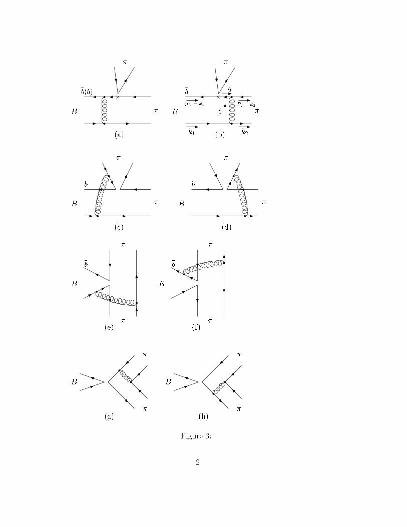
With the above brief discussion, the only thing left is to compute H for each diagram. There

are altogether 8 diagrams contributing to the B → ππ decays, which are shown in Figure 3.

They are the lowest order diagrams. In fact the diagrams without hard gluon exchange between

the spectator quark and other quarks are suppressed by the wave functions. The reason is that

the light quark in B meson is almost at rest. If there is no large momentum exchange with

other quarks, it carries almost zero momentum in the fast moving π, that is the end point

of pion wave function. In the next section, we will see that the pion wave function at the

zero point is always zero. The Sudakov form factor suppresses the large number of soft gluons

exchange to transfer large momentum. It is already shown that the hard gluon is really hard

in the numerical calculations of B → Kπ [18]. The value of αs/π is peaked below 0.2. And in

our following calculation of B → ππ decays this is also proved.

Let’s first calculate the usual factorizable diagrams (a) and (b). The four quark operators

indicated by a cross in the diagrams, are shown in the appendix A. There are two kinds of

operators. Operators O1, O2, O3, O4, O9, and O10 are (V − A)(V − A) currents, the sum of

their amplitudes is given as

Fe = −16πCFm2B

∫ 1

0dx1dx2

∫ ∞

0b1db1b2db2 φB(x1, b1)

×{[(1 + x2)φπ(x2, b2) + (1− 2x2)φ′π(x2, b2)rπ]

×αs(t1e)he(x1, x2, b1, b2) exp[−SB(t

1e)− S1

π(t1e)] + 2rπφ

′π(x2, b2)

× αs(t2e)he(x2, x1, b2, b1) exp[−SB(t

2e)− S1

π(t2e)]}

, (13)

where rπ = m0/mB = m2π/[mB(mu + md)]. CF = 4/3 is a color factor. The function

he(x1, x2, b1, b2) and the Sudakov form factors SB(ti) and Sπ(ti) are given in the appendix

7

B. The operators O5, O6, O7, and O8 have a structure of (V − A)(V + A). The sum of their

amplitudes is

F Pe = −32πCFm

2Brπ

∫ 1

0dx1dx2

∫ ∞

0b1db1b2db2 φB(x1, b1)

×{

[φπ(x2, b2) + (2 + x2)φ′π(x2, b2)rπ]αs(t

1e)he(x1, x2, b1, b2)

× exp[−SB(t1e)− S1

π(t1e)] + [x1φπ(x2, b2) + 2(1− x1)φ

′π(x2, b2)rπ]

× αs(t2e)he(x2, x1, b2, b1) exp[−SB(t

2e)− S1

π(t2e)]}

. (14)

They are proportional to the factor rπ. There are also factorizable annihilation diagrams (g)

and (h), where the B meson can be factored out. For the (V − A)(V − A) operators, their

contributions always cancel between diagram (g) and (h). But for the (V −A)(V +A) operators,

their contributions are sum of diagram (g) and (h).

F Pa = −64πCFm

2Brπ

∫ 1

0dx2dx3

∫ ∞

0b2db2b3db3αs(ta)ha(x2, x3, b2, b3)

× [2φπ(x2, b2)φ′π(x3, b3) + x2φπ(x3, b3)φ

′π(x2, b2)] exp[−S1

π(ta)− S2π(ta)] , (15)

These two diagrams can be cut in the middle of the diagrams. They provide the main strong

phase for non-leptonic B decays. Note that F Pa vanishes in the limit of m0 = 0. So the m0 term

in the pion wave function does not only have much effect on the branching ratios, but also the

CP asymmetries. Besides the factorizable diagrams, we can also calculate the non-factorizable

diagrams (c) and (d) and also the non-factorizable annihilation diagrams (e) and (f). In this

case, the amplitudes involve all the three meson wave functions. The integration over b3 can be

performed easily using δ function δ(b3 − b1) in diagram (c,d) and δ(b3 − b2) for diagram (e,f).

Me =32

3πCF

√

2Ncm2B

∫ 1

0dx1dx2 dx3

∫ ∞

0b1db1b2db2 φB(x1, b1)φπ(x2, b2)

×φπ(x3, b1)x2αs(td)hd(x1, x2, x3, b1, b2) exp[−SB(td)− S1π(td)− S2

π(td)] , (16)

Ma =32

3πCF

√

2Ncm2B

∫ 1

0dx1dx2 dx3

∫ ∞

0b1db1b2db2 φB(x1, b1)

×{

−[

x2φπ(x2, b2)φπ(x3, b2) + (x2 + x3)φ′π(x2, b2)φ

′π(x3, b2)r

2π

]

× αs(t1f)h

(1)f (x1, x2, x3, b1, b2) exp

[

−SB(t1f)− S1

π(t1f)− S2

π(t1f )]

+[

x2φπ(x2, b2)φπ(x3, b2) + (2 + x2 + x3)φ′π(x2, b2)φ

′π(x3, b2)r

2π

]

× αs(t2f)h

(2)f (x1, x2, x3, b1, b2)] exp[−SB(t

2f)− S1

π(t2f )− S2

π(t2f )]}

. (17)

8

Note that when doing the above integrations over xi and bi, we have to include the correspond-

ing Wilson coefficients Ci evaluated at the corresponding scale ti. The expression of Wilson

coefficients are channel dependent which are shown later in this section. The functions hi,

coming from the Fourier transform of H , are given in Appendix B. In the above equations, we

have used the assumption that x1 ≪ x2, x3. Since the light quark momentum fraction x1 in

B meson is peaked at the small region, while quark momentum fraction x2 of pion is peaked

at 0.5, this is not a bad approximation. After using this approximation, all the diagrams are

functions of k−1 = x1mB/

√2 of B meson only, independent of the variable of k+

1 . For example,

by calculating the diagrams (b) we shall demonstrate it.

〈π(P2)π(P3)|Ou†2 |B(pB)〉

∝∫

d4k1d4k2 φB(k1)φ

′π(k2)

q · P3

q2 ℓ2

=∫

d4k1d4k2 φB(k1)φ

′π(k2)

(P+2 − k+

1 )p−B

{2(P+2 − k+

1 )k−1 + k2

1T}{2(k+2 − k+

1 )k−1 + ℓ2T}

≃∫

d4k1d4k2 φB(k1)φ

′π(k2)

{

p−BP+2

(2P+2 k−

1 + k21T )(2k

−1 k

+2 + ℓ2T )

+O(

ΛQCD

m2B

)}

, (18)

where the momenta are assigned in Figure 3. The calculation from second formula to last one

is approximated as 〈k1〉 ≪ 〈k2〉. This approximation is equal to take the momenta of spectator

quark in the B meson as k1 = (0, k−1 ,k1T ). We neglect the last term which is higher order one

in terms of 1/mB expansion. Therefore the integration of eq.(5) is performed safely. Though we

calculated the above factorization formulae by one order in terms of αs, the radiative corrections

at the next order would emerge in forms of α2s ln(m/t), where m’s denote some scales, i.e. mB,

1/b, . . ., in the hard part H(t). Selecting t as the largest scale in m’s, the largest logarithm

in the next order corrections is killed. Accordingly, the scale ti’s in the above equations are

chosen as

t1e = max(√x2mB, 1/b1, 1/b2) , (19)

t2e = max(√x1mB, 1/b1, 1/b2) , (20)

td = max(√x1x2mB,

√x2x3mB, 1/b1, 1/b2) ,

t1f = max(√x2x3mB, 1/b1, 1/b2) ,

t2f = max(√x2x3mB,

√x2 + x3 − x2x3mB, 1/b1, 1/b2) ,

ta = max(√x2mB, 1/b2, 1/b3) . (21)

9

They are given the maximum values of the scales appeared in each diagram.

In the language of the above matrix elements for different diagrams eq.(13-17), the decay

amplitude for B0 → π+π− can be written as

M(B0 → π+π−) = fπFe

[

ξu

(

1

3C1 + C2

)

− ξt

(

C4 +1

3C3 + C10 +

1

3C9

)]

− fπFPe ξt

[

C6 +1

3C5 + C8 +

1

3C7

]

+ Me [ξuC1 − ξt(C3 + C9)]

+ Ma

[

ξuC2 − ξt

(

C3 + 2C4 + 2C6 +1

2C8 −

1

2C9 +

1

2C10

)]

− fBFaξt

[

1

3C5 + C6 −

1

6C7 −

1

2C8

]

, (22)

where ξu = V ∗ubVud, ξt = V ∗

tbVtd. The decay width is expressed as

Γ =G2

Fm3B

128π|M|2. (23)

The C ′is should be calculated at the appropriate scale ti using eq.(61,62) in the appendices.

The decay amplitude of the charge conjugate decay channel B0 → π+π− is the same as eq.(22)

except replacing the CKM matrix elements ξu to ξ∗u and ξt to ξ∗t under the phase convention

CP |B0〉 = |B0〉.The decay amplitude for B0 → π0π0 can be written as

−√2M(B0 → π0π0) = fπFe

[

ξu

(

C1 +1

3C2

)

+ξt

(

1

3C3 + C4 +

3

2C7 +

1

2C8 −

5

3C9 − C10

)]

+ fπFPe ξt

[

C6 +1

3C5 −

1

6C7 −

1

2C8

]

+ Me

[

ξuC2 − ξt(−C3 +3

2C8 +

1

2C9 +

3

2C10)

]

− Ma

[

ξuC2 − ξt

(

C3 + 2C4 + 2C6 +1

2C8 −

1

2C9 +

1

2C10

)]

+ fBFaξt

[

1

3C5 + C6 −

1

6C7 −

1

2C8

]

. (24)

The decay amplitude for B+ → π+π0 can be written as

√2M(B+ → π+π0) = fπFe

[

4

3ξu(C1 + C2)− ξt

(

2C10 + 2C9 −3

2C7 −

1

2C8

)]

− fπFPe ξt

[

3

2C8 +

1

2C7

]

+ Me

[

ξu(C1 + C2)−3

2ξt(C8 + C9 + C10)

]

. (25)

10

From the above equations (22,24,25), it is easy to see that we have the exact Isospin relation

for the three decays:

M(B0 → π+π−)−√2M(B0 → π0π0) =

√2M(B+ → π+π0). (26)

4 Numerical calculations and discussions of Results

In the numerical calculations we use [19]

Λ(f=4)

MS= 0.25 GeV, fπ = 0.13 GeV, fB = 0.19 GeV,

MB = 5.2792 GeV, MW = 80.41 GeV,

τB± = 1.65× 10−12 s, τB0 = 1.56× 10−12 s (27)

and

mu = 4.5 MeV, md = 1.8mu, (28)

which is relevant to taking m0 = 1.5 GeV. For the π wave function, we neglect the b dependence

part, which is not important in numerical analysis. We use

φπ(x) =3√2Nc

fπx(1 − x)[1 + aA(5(1− 2x)2 − 1)], (29)

with aA = 0.8, which is close to the Chernyak-Zhitnitsky (CZ) wave function [20]. For this

axial vector wave function the asymptotic wave function [21], aA ∼ 0 , is suggested from QCD

sum rules [22], diffractive dissociation of high momentum pions [23], the instanton model [24],

and pion distribution functions [25], etc., but we adopt aA = 0.8 according to the discussion

in ref. [26]. φ′π is chosen as asymptotic wave function

φ′π(x) =

3√2Nc

fπx(1− x)[1 + ap(5(1− 2x)2 − 1)], (30)

with aP = 0. For B meson, the wave function is chosen as

φB(x, b) = NBx2(1− x)2 exp

[

−M2B x2

2ω2b1

− 1

2(ωb2b)

2

]

, (31)

with ωb1 = ωb2 = 0.4 GeV [27], and NB = 91.745 GeV is the normalization constant. In

this work, we set ωb1 = ωb2 for simplicity. We would like to point out that the choice of the

meson wave functions as in eqs. (29-31) and the above parameters can not only explain the

11

experimental data of B → ππ, but also B → Kπ [18, 26], Dπ etc., which is the result of a

global fitting. However, since the predicted branching ratio of B → ππ is sensitive to the input

parameters fB, m0, aA, aP and ωb1, we will at first give the numerical results with the above

parameters, then we give the allowed parameter regions of fB, m0, aA, aP and ωb1 constrained

by the experimental data of B → π+π− presented by CLEO.

The diagrams (a) and (b) in Fig.3, calculated in eq.(13) correspond to the B → π transition

form factor FBπ(q2 = 0), where q = pB −P2. Our result is FBπ(0) = 0.25 to be consistent with

QCD sum rule one. This implies that PQCD can explain the transition form factor in the B

meson decays, which is different with the conclusion in ref.[12]. In that paper, because m0 was

not considered, perturbative contributions to FBπ(0) were predicted to be much smaller than

nonperturbative ones.

Although we take the CZ like wave function (aA = 0.8) for φπ, one finds that the above

parameters give the pion electromagnetic form factor to be consistent with the experimental

data. The pion electromagnetic form factor Fπ(Q2) in PQCD is given as [28, 29]

Fπ(Q2) = 16πCF

∫ 1

0dx2dx3

∫ ∞

0b2db2 b3db3 αs(t) he(x3, x2, b3, b2)

×{

x2Q2φπ(x2, b2)φπ(x3, b3) + 2m2

0(1− x2)φ′π(x2, b2)φ

′π(x3, b3)

}

× exp[−S1π(t)− S2

π(t)], (32)

where−Q2 is the momentum transfer in this system, the scale t is chosen as t = max(√x2Q, 1/b2, 1/b3),

and mB’s are replaced by Q in the he, S1π and S2

π. One may suspect that around x1, x2 ∼ 0,

the gluon and virtual quark propagators give rise to IR divergences which can not be canceled

by the wave functions. However, in PQCD, the transverse momenta kT save perturbative cal-

culations from the singularities around x1,2 ∼ 0. There are still IR divergences around kT ∼ 0,

but the Sudakov factor which can be calculated from QCD corrections does suppress such a

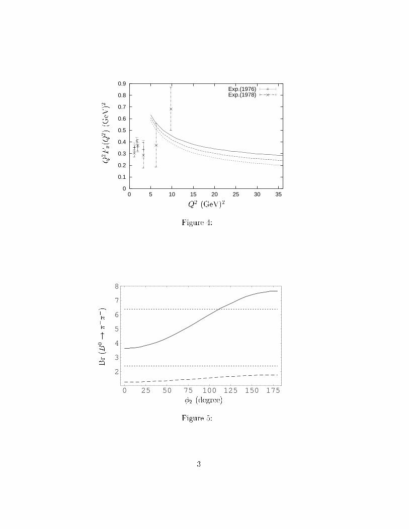
region, i.e., non-perturbative contributions, sufficiently. We show the Q2 dependence of Fπ(Q2)

(eq.(32)) in Figure 4 with the experimental data [30]. This figure shows that the parameters

we used don’t conflict with the data. We also show Fπ(Q2) for aA = 0.8, 0.4, and 0. It indicates

that Fπ(Q2) is fairly insensitive to aA.

12

The CKM parameters we used here are

|Vud| = 0.9740± 0.0010, |Vub/Vcb| = 0.08± 0.02,

|Vcb| = 0.0395± 0.0017, |V ∗tbVtd| = 0.0084± 0.0018.

(33)

We leave the CKM angle φ2 as a free parameter. φ2’s definition is [31]

φ2 = arg

[

− VtdV∗tb

VudV∗ub

]

. (34)

In this parameterization, the decay amplitude of B → ππ can be written as

M = V ∗ubVudT − V ∗

tbVtdP

= V ∗ubVudT

[

1 + zei(φ2+δ)]

, (35)

where z =∣

∣

∣

∣

V ∗tbVtd

V ∗ub

Vud

∣

∣

∣

∣

∣

∣

∣

PT

∣

∣

∣, and δ is the relative strong phase between tree (T) diagrams and penguin

diagrams (P). z and δ can be calculated from PQCD. For example, in B0 → π+π− decay, we

get z = 30%, and δ = 130◦, if we use the above parameters. Here in PQCD approach, the

strong phases come from the non-factorizable diagrams and annihilation type diagrams (see (c)

∼ (h) in Figure 3). The internal quarks and gluons can be on mass shell providing the strong

phases. This can also be seen from eq.(57-60), where the the modified Bessel function K0(−if)

has imaginary part. Numerical analysis also shows that the main contribution to the relative

strong phase δ comes from the annihilation diagrams, (g) and (h) in Figure 3. From the figure,

we can see that they are factorizable diagrams. B meson annihilates to qq quark pair then

decays to ππ final states. The intermediate qq quark pair represent a number of resonance

states, which implies final state interaction. In perturbative calculations, the two quark lines

can be cut providing the imaginary part. The importance of these diagrams also makes the

contribution of penguin diagrams more important than previously expected.

This mechanism of producing CP violation strong phase is very different from the so-called

Bander-Silverman-Soni (BSS) mechanism [32], where the strong phase comes from the per-

turbative penguin diagrams. The contribution of BSS mechanism to the direct CP violation

in B → π+π− is only in the order of few percent [5, 7]. It is higher order corrections (αs

suppressed) in our PQCD approach. Therefore in our approach we can safely neglect this

contribution. The corresponding charge conjugate B decay is

M = VubV∗udT − VtbV

∗tdP

= VubV∗udT

[

1 + zei(−φ2+δ)]

. (36)

13

Therefore the averaged branching ratio for B → ππ is

Br = (|M|2 + |M|2)/2

= |VubV∗udT |2

[

1 + 2z cos φ2 cos δ + z2]

. (37)

From this equation, we know that the averaged branching ratio is a function of CKM angle φ2,

if z cos δ 6= 0.

The averaged branching ratio of B0 → π+π− decay which is predicted from the formulae in

the previous section is shown as a function of φ2 in Figure 5. To consider m0 required from chiral

symmetry is essentially different with previous paper [11]. This figure shows that m0 enhances

the branching ratio to agree with the experimental data. There is a significant dependence

on the CKM angle φ2. The branching ratio of B0 → π+π− is larger when φ2 is larger. The

reason is that the penguin contribution is not small. The CLEO measured branching ratio of

B → π+π− [6]

Br(B → π+π−) = (4.3+1.6−1.4 ± 0.5)× 10−6, (38)

is in good agreement with our predictions. This prefer a lower value of φ2. However, the

predicted branching ratio is sensitive to the parameters of input. Especially it is sensitive to

fB, m0 and the meson wave functions. Therefore, it is unlikely to use this single channel to

determine the CKM angle φ2.

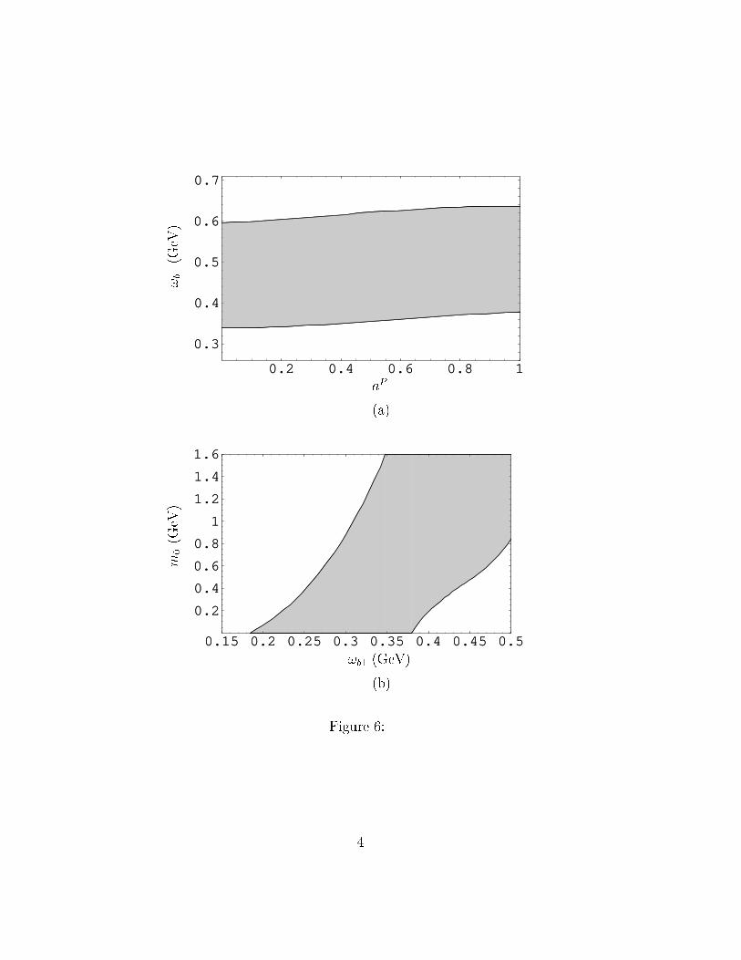
The branching ratios of B → ππ are sensitive to some input parameters. We give the

parameter regions allowed by the experimental data in eq. (38). Rerevant parameter are m0,

aP , and ωb1. Others are specified in the begining of this section. Here we check the sensitivity

of our calculation on parameter m0, aP , and ωb1. First we fix m0 = 1.5 GeV and show the

allowed region for aP and ωb1. This is shown in Figure 6(a). One finds that the branching ratio

is fairly insensitive to aP . Second we fix aP = 0 and show the allowed region for ωb1 and m0.

This is shown in Figure 6(b). We see that the allowed region for ωb1 and m0 is quite large. The

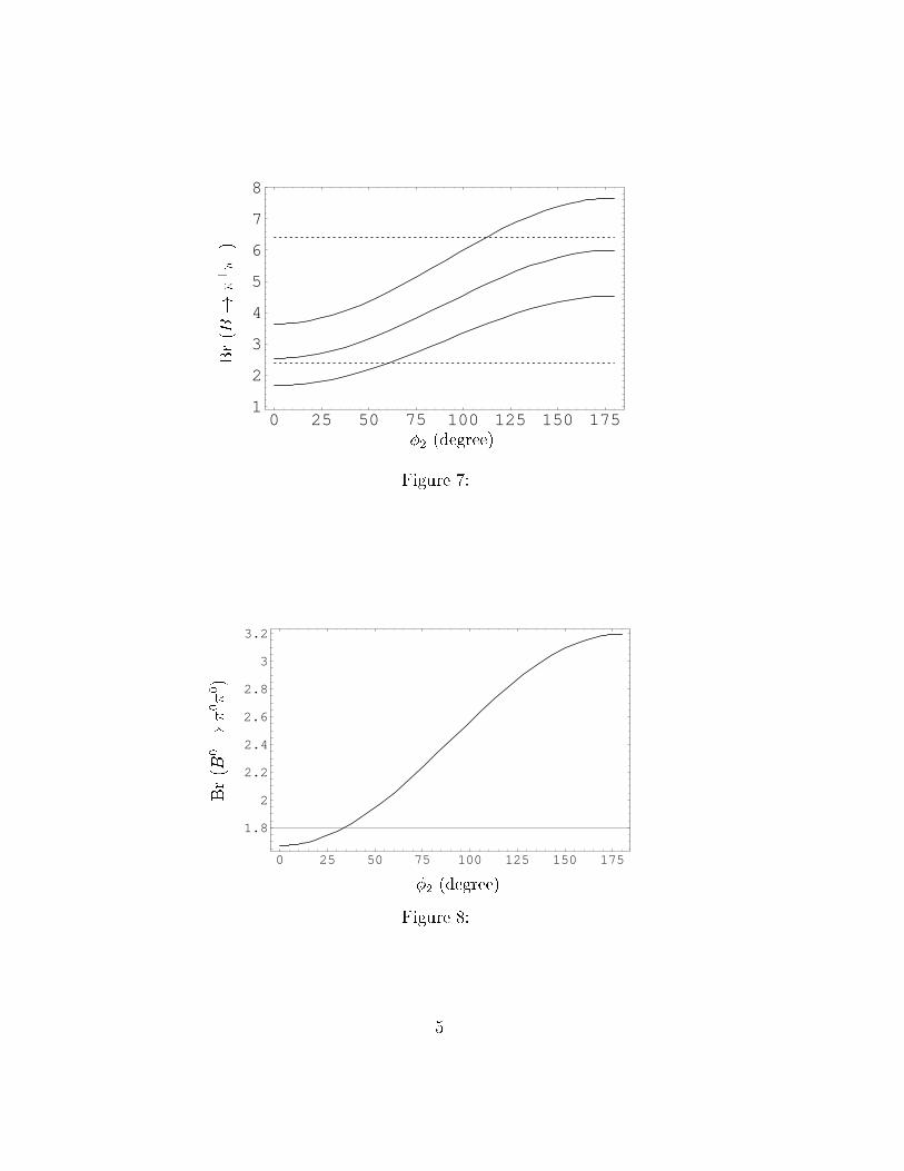
dependence on aA for the branching ratio of B → π+π− is given in Figure 7. As discussed in

ref. [26], the central value of the experimental data RD = Br(B− → D0π−)/Br(B0d → D+π−)

requires aA = 0.8, but this figure indicates that B → π+π− decay mode gives no significant

restriction on aA. Therefore, these figures show that the above set of parameters we choose for

Figure 5 is in the allowed region, and that parameter space producing the experimental data,

eq. (38), is quite large.

14

The branching ratio of B+ → π+π0 has little dependence on φ2. It is easy to understand

since there is only one dominant contribution from tree diagrams. The QCD penguin contribu-

tion is canceled by isospin relation and the electroweak contribution is very small giving only a

slight dependence on φ2. The branching ratio of this decay is predicted as 3× 10−6, using the

parameters we list in the beginning of this section.

For the decay of B0 → π0π0, the situation is similar to that of B0 → π+π−. There are

large contributions from both tree and penguin diagrams. We show the averaged branching

ratio of B0 → π0π0 as a function of φ2 in Figure 8. Although the branching ratio is small, the

dependence of φ2 is significant. The predicted branching ratio of B0 → π0π0 is less than 10−6.

This is difficult for the B factories to measure the separate branching ratios of B0 and B0. In

this case, the proposed isospin method to measure the CKM angle φ2 [33] does not work in the

B factories, since it requires the measurement of B0 → π0π0 and B0 → π0π0.

Using eq.(35,36), the direct CP violating parameter is

AdirCP =

|M|2 − |M|2|M|2 + |M|2

=−2z sinφ2 sin δ

1 + 2z cosφ2 cos δ + z2. (39)

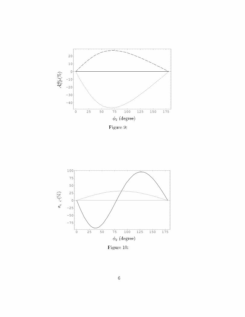
The direct CP asymmetry is nearly proportional to sin φ2. We show the direct CP violation

parameters (percentage) as a function of φ2 in figure 9. Unlike the averaged branching ratios,

the predicted CP violation in B decays does not depend much on the wave functions. They

cancel each between the charge conjugate states shown in the above equation. The direct CP

violation parameter of B0 → π+π− and π0π0 can be very large, which can be as large as

40%, and 20% when φ2 is near 70◦. Because there is no annihilation diagram contribution

in B+ → π+π0, the penguin contribution is negligible. The direct CP violation parameter of

B+ → π+π0 is also very small. It is a horizontal line in Figure 9.

For the neutral B0 decays, there is more complication from the B0-B0 mixing. The CP

asymmetry is time dependent [5, 34]:

ACP (t) ≃ AdirCP cos(∆mt) + aǫ+ǫ′ sin(∆mt), (40)

where ∆m is the mass difference of the two mass eigenstates of neutral B mesons. The direct CP

violation parameter AdirCP is already defined in eq.(39). While the mixing-related CP violation

15

parameter is defined as

aǫ+ǫ′ =−2Im(λCP )

1 + |λCP |2, (41)

where

λCP =V ∗tbVtd〈f |Heff |B0〉

VtbV ∗td〈f |Heff |B0〉 . (42)

Using equations (35,36), we can derive as

λCP = e2iφ21 + zei(δ−φ2)

1 + zei(δ+φ2). (43)

Usually, people believe that the penguin diagram contribution is suppressed comparing with the

tree contribution, i.e. z ≪ 1. Such that λCP ≃ exp[2iφ2], aǫ+ǫ′ = − sin 2φ2, and AdirCP ≃ 0. That

is the previous idea of extracting sin 2φ2 from the CP measurement of B0 → π+π−. However,

z is not very small. From Figure 10, we can see that aǫ+ǫ′ is not a simple − sin 2φ2 behavior

due to the so called penguin pollution.

If we integrate the time variable t, we will get the total CP asymmetry as

ACP =1

1 + x2Adir

CP +x

1 + x2aǫ+ǫ′, (44)

with x = ∆m/Γ ≃ 0.723 for the B0-B0mixing in SM [19].

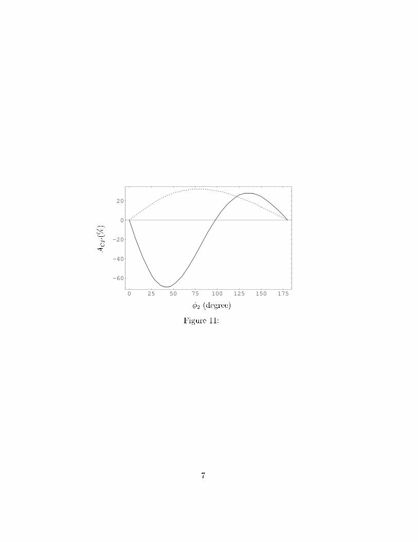
The integrated CP asymmetries of B0 → π+π− and B0 → π0π0 are shown in Figure 11.

Unlike the averaged branching ratios, the CP asymmetry is not sensitive to the wave functions,

since these parameter dependences canceled out. It is rather stable. If we can measure the

integrated CP asymmetry from the experiments, then we can use this figure to determine the

value of φ2.

5 Summary

We performed the calculations of B0 → π+π−, B+ → π+π0, and B0 → π0π0 decays, in a

perturbative QCD approach. In this approach, we calculate the non-factorizable contribu-

tions and annihilation type contributions in addition to the usual factorizable contributions.

The predicted branching ratios of B0 → π+π− is in good agreement with the experimental

measurement by the CLEO Collaboration.

We found that the annihilation contributions were not as small as expected in a simple

argument. The annihilation diagram, which provides the dominant strong phases, plays an

16

important role in the CP violation asymmetries. We expect large direct CP asymmetries in

the decay of B0 → π+π−, and B0 → π0π0. The ordinary method of measuring the CKM angle

φ2 will suffer from the large penguin pollution. The isospin method does not help, since the B

factories can not measure well the small branching ratio of B0 → π0π0. Working in our PQCD

approach, we give the predicted dependence of CP asymmetry on CKM angle φ2. Using this

dependence, the current running B factories in KEK and SLAC will be able to measure the

CKM angle φ2.

Acknowledgments

We thank our PQCD group members: Y.Y. Keum, E. Kou, T. Kurimoto, H.N. Li, T. Mo-

rozumi, A.I. Sanda, N. Sinha, R. Sinha, and T. Yoshikawa for helpful discussions. This work

was supported by the Grant-in-Aid for Scientific Research on Priority Areas (Physics of CP

violation). C.D. L. and M.Z. Y. thanks JSPS for support. K. U. thanks JSPS for partial

support.

A Wilson Coefficients

In this appendix we present the weak effective Hamiltonian Heff which we used to calculate the

hard part H(t) in eq.(2). The Heff for the ∆B = 1 transitions at the scale smaller than mW is

given as

Heff =GF√2

[

VubV∗ud (C1O

u1 + C2O

u2 )− VtbV

∗td

(

10∑

i=3

CiOi + CgOg

)]

. (45)

We specify below the operators in Heff for b → d:

Ou1 = dαγ

µLuβ · uβγµLbα , Ou2 = dαγ

µLuα · uβγµLbβ ,

O3 = dαγµLbα ·∑q′ q

′βγµLq

′β , O4 = dαγ

µLbβ ·∑

q′ q′βγµLq

′α ,

O5 = dαγµLbα ·∑q′ q

′βγµRq′β , O6 = dαγ

µLbβ ·∑

q′ q′βγµRq′α ,

O7 = 32dαγ

µLbα ·∑q′ eq′ q′βγµRq′β , O8 = 3

2dαγ

µLbβ ·∑

q′ eq′ q′βγµRq′α ,

O9 = 32dαγ

µLbα ·∑q′ eq′ q′βγµLq

′β , O10 = 3

2dαγ

µLbβ ·∑

q′ eq′ q′βγµLq

′α .

(46)

Here α and β are the SU(3) color indices; L and R are the left- and right-handed projection

operators with L = (1− γ5), R = (1+ γ5). The sum over q′ runs over the quark fields that are

17

active at the scale µ = O(mb), i.e., (q′ǫ{u, d, s, c, b}).

The PQCD approach works well for the leading twist approximation and leading double

logarithm summation. For the Wilson coefficients, we will also use the leading logarithm

summation for the QCD corrections, although the next-to-leading order calculations already

exist in the literature [16]. This is the consistent way to cancel the explicit µ dependence in

the theoretical formulae.

At mW scale, the Wilson coefficients are evaluated for leading order as:

C2w = 1,

Ciw = 0, i = 1, 8, 10,

C3w = −αs(mW )

24πE0 +

α

6π

1

sin2 θW(2B0 + C0),

C4w =αs(mW )

8πE0,

C5w = −αs(mW )

24πE0,

C6w =αs(mW )

8πE0,

C7w =α

6π(4C0 +D0),

C9w =α

6π

[

4C0 +D0 +1

sin2 θW(10B0 − 4C0)

]

, (47)

where

B0 =1

4

(

x

1− x+

x

(x− 1)2ln x

)

,

C0 =x

8

(

x− 6

x− 1+

3x+ 2

(x− 1)2ln x

)

,

D0 = −4

9ln x+

−19x3 + 25x2

36(x− 1)3+

x2(5x2 − 2x− 6)

18(x− 1)4ln x,

E0 = −2

3ln x+

x(x2 + 11x− 18)

12(x− 1)3+

x2(4x2 − 16x+ 15)

6(x− 1)4ln x, (48)

with x = m2t/m

2W .

If the scale mb < t < mW , then we evaluate the Wilson coefficients at t scale using leading

logarithm running equations (61), in the appendix C. In numerical calculations, we use αs =

4π/[β1 ln(t2/Λ

(5)QCD

2)] which is the leading order expression with Λ

(5)QCD = 193MeV, derived from

Λ(4)QCD = 250MeV. Here β1 = (33 − 2nf )/3, with the appropriate number of active quarks nf .

nf = 5 when scale t is larger than mb.

18

The Wilson coefficients evaluated at t = mb = 4.8GeV scale using the above equations are

C1 = −0.27034, C2 = 1.11879,

C3 = 0.01261, C4 = −0.02695,

C5 = 0.00847, C6 = −0.03260,

C7 = 0.00109, C8 = 0.00040,

C9 = −0.00895, C10 = 0.00216.

(49)

If the scale t < mb, then we evaluate the Wilson coefficients at t scale using the input

of eq.(49), and the formulae in appendix D for four active quarks (nf = 4) (again in leading

logarithm approximation).

B Formulas for the hard part calculations

In this appendix we present the explicit expression of the formulas we used in section 3. First,

we show the exponent s(k, b) appearing in eq. (53-55). It is given, in terms of the variables,

q ≡ ln (k/Λ) , b ≡ ln(1/bΛ) (50)

by

s(k, b) =2

3β1

[

q ln

(

q

b

)

− q + b

]

+A(2)

4β21

(

q

b− 1

)

−[

A(2)

4β21

− 1

3β1(2γE − 1− ln 2)

]

ln

(

q

b

)

. (51)

The above coefficients β1 and A(2) are

β1 =33− 2nf

12

A(2) =67

9− π2

3− 10

27nf +

8

3β1 ln

(

eγE

2

)

, (52)

where γE is the Euler constant.

Note that s is defined for q ≥ b, and set to zero for q < b. As a similar treatment, the

complete Sudakov factor exp(−S) is set to unity, if exp(−S) > 1, in the numerical analysis.

This corresponds to a truncation at large kT , which spoils the on-shell requirement for the light

valence quarks. The quark lines with large kT should be absorbed into the hard scattering

amplitude, instead of the wave functions.

19

e−SB(t), e−S1π(t), and e−S2

π(t) used in the amplitudes are expressions abbreviated to combine

the Sudakov factor and single ultraviolet logarithms associated with the B and π meson wave

functions. The exponents are defined as

SB(t) = s(

x1mB/√2, b1

)

− 1

β1ln

ln(t/Λ)

− ln(b1Λ), (53)

S1π(t) = s

(

x2mB/√2, b2

)

+ s(

(1− x2)mB/√2, b2

)

− 1

β1ln

ln(t/Λ)

− ln(b2Λ), (54)

S2π(t) = s

(

x3mB/√2, b3

)

+ s(

(1− x3)mB/√2, b3

)

− 1

β1ln

ln(t/Λ)

− ln(b3Λ). (55)

The last term of each equations is the integration result of the last term in eq.(2).

The function hi’s, coming from the Fourier transform of hard part H , are given as,

he(x1, x2, b1, b2) = K0 (√x1x2mBb1) [θ(b1 − b2)K0 (

√x2mBb1) I0 (

√x2mBb2)

+θ(b2 − b1)K0 (√x2mBb2) I0 (

√x2mBb1)] , (56)

hd(x1, x2, x3, b1, b2) = K0 (−i√x2x3mBb2) [θ(b1 − b2)K0 (

√x1x2mBb1) I0 (

√x1x2mBb2)

+θ(b2 − b1)K0 (√x1x2mBb2) I0 (

√x1x2mBb1)] , (57)

h(1)f (x1, x2, x3, b1, b2) = K0 (−i

√x2x3mBb1)

× [θ(b1 − b2)K0 (−i√x2x3mBb1)J0 (

√x2x3mBb2)

+θ(b2 − b1)K0 (−i√x2x3mBb2) J0 (

√x2x3mBb1)] , (58)

h(2)f (x1, x2, x3, b1, b2) = K0

(√x2 + x3 − x2x3mBb1

)

× [θ(b1 − b2)K0 (−i√x2x3mBb1)J0 (

√x2x3mBb2)

+θ(b2 − b1)K0 (−i√x2x3mBb2) J0 (

√x2x3mBb1)] , (59)

ha(x2, x3, b2, b3) = K0 (−i√x2x3mBb3) [θ(b2 − b3)K0 (−i

√x2mBb2)J0 (

√x2mBb3)

+ θ(b3 − b2)K0 (−i√x2mBb3)J0 (

√x2mBb2)] , (60)

with J0 the Bessel function and K0, I0 modified Bessel functions K0(−ix) = −(π/2)Y0(x) +

i(π/2)J0(x).

C Wilson coefficients running equations above mb scale

In this appendix, we list formulas for renormalization group running from mW scale to t scale,

where t > mb. These formulas are derived from the leading logarithm QCD corrections with

20

five active quarks [16].

C1 =1

2

(

η−6/23 − η12/23)

,

C2 =1

2

(

η−6/23 + η12/23)

,

C3 = 0.0510η−0.4086 − 0.0714η−6/23 + 0.0054η−0.1456

−0.1403η0.4230 − 0.0113η0.8994 + 1/6η12/23

+C3w(0.2868η−0.4086 + 0.0491η−0.1456 + 0.6579η0.4230 + 0.0061η0.8994)

+C4w(0.3287η−0.4086 + 0.0424η−0.1456 − 0.3263η0.4230 − 0.0448η0.8994)

+C5w(−0.0629η−0.4086 + 0.1629η−0.1456 − 0.1846η0.4230 + 0.0846η0.8994)

+C6w(0.0447η−0.4086 − 0.0063η−0.1456 − 0.2610η0.4230 + 0.2226η0.8994)

+C9w

(

−0.0325η−0.4086 + 0.0357η−6/23 − 0.0016η−0.1456

+ 0.2342η0.4230 − 0.25η12/23 + 0.0141η0.8994)

+C7w

(

−0.0063η−0.4086 + 0.0163η−0.1456 − 0.0185η0.4230 + 0.0085η0.8994)

,

C4 = 0.0984η−0.4086 − 0.0714η−6/23 + 0.0026η−0.1456

+0.1214η0.4230 − 1/6η12/23 + 0.0156η0.8994

+C3w(0.5539η−0.4086 + 0.0239η−0.1456 − 0.5693η0.4230 − 0.0085η0.8994)

+C4w(0.6348η−0.4086 + 0.0206η−0.1456 + 0.2823η0.4230 + 0.0623η0.8994)

+C5w(−0.1215η−0.4086 + 0.0793η−0.1456 + 0.1597η0.4230 − 0.1175η0.8994)

+C6w(0.0864η−0.4086 − 0.0031η−0.1456 + 0.2259η0.4230 − 0.3092η0.8994)

+C9w

(

−0.0627η−0.4086 + 0.0357η−6/23 − 0.0008η−0.1456

− 0.2027η0.4230 + 0.25η12/23 − 0.0196η0.8994)

+C7w

(

−0.0122η−0.4086 + 0.0079η−0.1456 + 0.0160η0.4230 − 0.0117η0.8994)

,

C5 = −0.0397η−0.4086 + 0.0304η−0.1456 + 0.0117η0.4230 − 0.0025η0.8994

+C3w(−0.2233η−0.4086 + 0.2767η−0.1456 − 0.0547η0.4230 + 0.0013η0.8994)

+C4w(−0.2559η−0.4086 + 0.2385η−0.1456 + 0.0271η0.4230 − 0.0098η0.8994)

+C5w(0.0490η−0.4086 + 0.9171η−0.1456 + 0.0154η0.4230 + 0.0185η0.8994)

+C6w(−0.0348η−0.4086 − 0.0357η−0.1456 + 0.0217η0.4230 + 0.0488η0.8994)

21

+C9w

(

0.0253η−0.4086 − 0.0089η−0.1456 − 0.0195η0.4230 + 0.0031η0.8994)

+C7w

(

0.0049η−0.4086

+ 0.0917η−0.1456 − 0.1η−3/23 + 0.0015η0.4230 + 0.0019η0.8994)

,

C6 = 0.0335η−0.4086 − 0.0112η−0.1456 + 0.0239η0.4230 − 0.0462η0.8994

+C3w(0.1885η−0.4086 − 0.1017η−0.1456 − 0.1120η0.4230 + 0.0251η0.8994)

+C4w(0.2160η−0.4086 − 0.0877η−0.1456 + 0.0555η0.4230 − 0.1839η0.8994)

+C5w(−0.0414η−0.4086 − 0.3370η−0.1456 + 0.0314η0.4230 + 0.3469η0.8994)

+C6w(0.0294η−0.4086 + 0.0131η−0.1456 + 0.0444η0.4230 + 0.9131η0.8994)

+C9w

(

−0.0213η−0.4086 + 0.0033η−0.1456 − 0.0399η0.4230 + 0.0579η0.8994)

+C7w

(

−0.0041η−0.4086 − 0.0337η−0.1456 + η−3/23/30 + 0.0031η0.4230

+ 0.0347η0.8994 − η24/23/30)

,

C7 = C7wη−3/23,

C8 =1

3C7w

(

−η−3/23 + η24/23)

,

C9 =1

2C9w

(

η−6/23 + η12/23)

,

C10 =1

2C9w

(

η−6/23 − η12/23)

, (61)

where η = αs(t)/αs(mW ).

D Wilson coefficients running equations below mb scale

In this appendix, we list formulas for renormalization group running from mb scale to t scale,

where t < mb. These formulas are derived from the leading logarithm QCD corrections with

four active quarks [16].

CC1 =1

2C2

(

ζ−6/25 − ζ12/25)

+1

2C1

(

ζ−6/25 + ζ12/25)

,

CC2 =1

2C2

(

ζ−6/25 + ζ12/25)

+1

2C1

(

ζ−6/25 − ζ12/25)

,

CC3 = C4

(

0.3606ζ−0.3469 + 0.03166ζ−0.1317 − 0.3626ζ0.4201 − 0.0297ζ0.8451)

+C10

(

0.0149ζ−0.3469 − 0.0020ζ−0.1317 − 0.4981ζ0.4201 + 0.5ζ12/25 − 0.0148ζ0.8451)

+C2

(

0.0651ζ−0.3469 − 0.0833ζ−6/25

22

+ 0.0046ζ−0.1317 − 0.2265ζ0.4201 + 0.25ζ12/25 − 0.0099ζ0.8451)

+C3

(

0.3308ζ−0.3469 + 0.0356ζ−0.1317 + 0.6337ζ0.4201 − 0.0001ζ0.8451)

+C1

(

0.0502ζ−0.3469 − 0.0833ζ−6/25 + 0.0066ζ−0.1317 + 0.2717ζ0.4201

−0.25ζ12/25 + 0.0049ζ0.8451)

+ C9

(

−0.0149ζ−0.3469

+0.0020ζ−0.1317 + 0.4981ζ0.4201 − 0.5ζ12/25 + 0.0148ζ0.8451)

+C5

(

−0.0598ζ−0.3469 + 0.1371ζ−0.1317 − 0.1473ζ0.4201 + 0.0700ζ0.8451)

+C6

(

0.0377ζ−0.3469 − 0.0045ζ−0.1317 − 0.2210ζ0.4201 + 0.18775ζ0.8451)

+C7

(

−0.0150ζ−0.3469 + 0.0343ζ−0.1317 − 0.0368ζ0.4201 + 0.0175ζ0.8451)

+C8

(

0.009ζ−0.3469 − 0.0011ζ−0.1317 − 0.0553ζ0.4201 + 0.0469ζ0.8451)

,

CC4 = C6

(

0.0640ζ−0.3469 − 0.0021ζ−0.1317 + 0.2018ζ0.4201 − 0.2637ζ0.8451)

+C5

(

−0.10156ζ−0.3469 + 0.06538ζ−0.1317 + 0.1345ζ0.4201 − 0.09836ζ0.8451)

+C9

(

−0.02528ζ−0.3469 + 0.0009ζ−0.1317

− 0.4549ζ0.4201 + 0.5ζ12/25 − 0.0207ζ0.8451)

+C1

(

0.08515ζ−0.3469 − 0.0833ζ−6/25 + 0.0031ζ−0.1317

− 0.24809ζ0.4201 + 0.25ζ12/25 − 0.00688ζ0.8451)

+C3

(

0.5615ζ−0.3469 + 0.01699ζ−0.1317 − 0.5787ζ0.4201 + 0.0002ζ0.8451)

+C2

(

0.1104ζ−0.3469 − 0.0833ζ−6/25

+0.0022ζ−0.1317 + 0.2068ζ0.4201 − 0.25ζ12/25 + 0.0139ζ0.8451)

+C10

(

0.0253ζ−0.3469 − 0.0009ζ−0.1317

+ 0.4549ζ0.4201 − 0.5ζ12/25 + 0.0207ζ0.8451)

+C4

(

0.6121ζ−0.3469 + 0.0151ζ−0.1317 + 0.3311ζ0.4201 + 0.0417ζ0.8451)

+C8

(

0.0160ζ−0.3469 − 0.0005ζ−0.1317 + 0.0505ζ0.4201 − 0.0659ζ0.8451)

+C7

(

−0.0254ζ−0.3469 + 0.0163ζ−0.1317 + 0.0336ζ0.4201 − 0.0246ζ0.8451)

,

CC5 = C4

(

−0.2291ζ−0.3469 + 0.2167ζ−0.1317 + 0.0192ζ0.4201 − 0.0067ζ0.8451)

+C10

(

−0.0095ζ−0.3469 − 0.0136ζ−0.1317 + 0.0264ζ0.4201 − 0.0034ζ0.8451)

+C2

(

−0.0413ζ−0.3469 + 0.0316ζ−0.1317 + 0.0120ζ0.4201 − 0.0022ζ0.8451)

+C3

(

−0.2102ζ−0.3469 + 0.2438ζ−0.1317 − 0.0336ζ0.4201)

23

+C1

(

−0.0319ζ−0.3469 + 0.0452ζ−0.1317 − 0.0144ζ0.4201 + 0.0011ζ0.8451)

+C9

(

0.0095ζ−0.3469 + 0.0136ζ−0.1317 − 0.0264ζ0.4201 + 0.0034ζ0.8451)

+C5

(

0.0380ζ−0.3469 + 0.9382ζ−0.1317 + 0.0078ζ0.4201 + 0.0159ζ0.8451)

+C6

(

−0.0240ζ−0.3469 − 0.0305ζ−0.1317 + 0.0117ζ0.4201 + 0.0427ζ0.8451)

+C8

(

−0.0060ζ−0.3469 − 0.0076ζ−0.1317 + 0.0029ζ0.4201 + 0.0107ζ0.8451)

+C7

(

0.0095ζ−0.3469 + 0.2346ζ−0.1317

− 0.25ζ−3/25 + 0.0020ζ0.4201 + 0.0040ζ0.8451)

,

CC6 = C4

(

0.1825ζ−0.3469 − 0.0784ζ−0.1317 + 0.0449ζ0.4201 − 0.14894ζ0.8451)

+C10

(

0.0075ζ−0.3469 + 0.0049ζ−0.1317 + 0.0617ζ0.4201 − 0.07412ζ0.8451)

+C2

(

0.0329ζ−0.3469 − 0.0114ζ−0.1317 + 0.0280ζ0.4201 − 0.0495ζ0.8451)

+C3

(

0.1674ζ−0.3469 − 0.0882ζ−0.1317 − 0.0784ζ0.4201 − 0.0007ζ0.8451)

+C1

(

0.0254ζ−0.3469 − 0.0163ζ−0.1317 − 0.0336ζ0.4201 + 0.0246ζ0.8451)

+C9

(

−0.0075ζ−0.3469 − 0.0049ζ−0.1317 − 0.0617ζ0.4201 + 0.07412ζ0.8451)

+C5

(

−0.0303ζ−0.3469 − 0.3395ζ−0.1317 + 0.0182ζ0.4201 + 0.35157ζ0.8451)

+C6

(

0.0191ζ−0.3469 + 0.0110ζ−0.1317 + 0.0274ζ0.4201 + 0.94253ζ0.8451)

+C8

(

0.0048ζ−0.3469 + 0.0028ζ−0.1317 + 0.0068ζ0.4201

+ 0.2356ζ0.8451 − 0.25ζ24/25)

+ C7

(

−0.0076ζ−0.3469 − 0.0849ζ−0.1317

+0.0833ζ−3/25 + 0.0046ζ0.4201 + 0.0879ζ0.8451 − 0.0833ζ24/25)

,

CC7 = C7ζ−3/25,

CC8 = C7

(

−ζ−3/25 + ζ24/25)

/3.+ C8ζ24/25,

CC9 = C10

(

0.5ζ−6/25 − 0.5ζ12/25)

+ C9

(

0.5ζ−6/25 + 0.5ζ12/25)

,

CC10 = C9

(

0.5ζ−6/25 − 0.5ζ12/25)

+ C10

(

0.5ζ−6/25 + 0.5ζ12/25)

, (62)

where ζ = αs(t)/αs(mB). Here Λ(4)QCD = 250MeV.

References

[1] See for example: I.I. Bigi, A.I. Sanda, CP violation, Cambridge.

24

[2] M. Wirbel, B. Stech, M. Bauer, Z. Phys. C29, 637 (1985); M. Bauer, B. Stech, M. Wirbel,

Z. Phys. C34, 103 (1987); L.-L. Chau, H.-Y. Cheng, W.K. Sze, H. Yao, B. Tseng, Phys.

Rev. D43, 2176 (1991), Erratum: D58, 019902 (1998).

[3] A. Ali, G. Kramer and C.D. Lu, Phys. Rev. D58, 094009 (1998); C.D. Lu, Nucl. Phys.

Proc. Suppl. 74, 227-230 (1999).

[4] Y.-H. Chen, H.-Y. Cheng, B. Tseng, K.-C. Yang, Phys. Rev. D60, 094014 (1999); H.-Y.

Cheng, K.-C. Yang, hep-ph/9910291.

[5] A. Ali, G. Kramer and C.D. Lu, Phys. Rev. D59, 014005 (1999); C.D. Lu, Invited talk at

3rd International Conference on B Physics and CP Violation (BCONF99), Taipei, Taiwan,

3-7 Dec 1999, hep-ph/0001321.

[6] D. Cronin-Hennessy, et al., CLEO Collaboration, hep-ex/0001010.

[7] M. Beneke, G. Buchalla, M. Neubert, C.T. Sachrajda, Phys. Rev. Lett. 83, 1914 (1999).

[8] H.N. Li, H.L. Yu, Phys. Rev. Lett. 74, 4388 (1995); Phys. Lett. B353, 301 (1995); H.n. Li,

ibid, 348, 597 (1995); Phys. Rev. D53, 2486 (1996).

[9] H.-n. Li, B. Tseng, Phys. Rev. D57, 443 (1998).

[10] H. n. Li, Phys. Lett. B348, 597 (1995).

[11] M. Dahm, R. Jakob, P. Kroll, Z. Phys. C68, 595 (1995).

[12] T. Feldmann and P. Kroll, Eur. Phys. J. C12, 99(2000)

[13] C.H. Chang, H.N. Li, Phys. Rev. D55, 5577 (1997); T.W. Yeh and H.N. Li, Phys. Rev.

D56, 1615 (1997).

[14] G.P. Lepage and S. Brodsky, Phys. Rev. D22, 2157 (1980).

[15] J. Botts and G. Sterman, Nucl. Phys. B225, 62 (1989).

[16] For a review, see G. Buchalla, A.J. Buras, M.E. Lautenbacher, Rev. Mod. Phys. 68, 1125

(1996).

25

[17] H.N. Li, Phys. Rev. D52, 3958 (1995).

[18] Y.Y. Keum, H.-n. Li, A.I. Sanda, preprint KEK-TH-642, NCKU-HEP-00-01, hep-

ph/0004004.

[19] Particle Data Group, Eur. Phys. J. C3, 1 (1998).

[20] V. L. Chernyak, A. R. Zhitnitsky, Phys. Rept. 112, 173 (1984)

[21] P. Kroll and M. Raulfs, Phys. Lett. B387, 848 (1996); S.J. Brodsky, C.R. Ji, A. Pang,

D.G. Robertson, Phys. Rev. D57, 245 (1998); I.V. Musatov and A.V. Radyushkin, Phys.

Rev. D56, 2713 (1997).

[22] A. P. Bakulev and S. V. Mikhailov, Mod. Phys. Lett. A11 (1996) 1611; V. Braun and

I. Halperin, Phys. Lett. B328 (1994) 457.

[23] D. Ashery [E791 Collaboration], hep-ex/9910024.

[24] V. Y. Petrov, M. V. Polyakov, R. Ruskov, C. Weiss and K. Goeke, Phys. Rev. D59 (1999)

114018.

[25] T. Huang, B.-Q. Ma, Q.-X. Shen, Phys. Rev. D49, 1490 (1994); F.-G. Cao, T. Huang,

B.-Q. Ma, Phys. Rev. D53, 6582 (1996); R. Jakob, P. Kroll, M. Raulfs, J. Phys. G22, 45

(1996).

[26] Y.Y. Keum, H.-n. Li, A.I. Sanda, hep-ph/0004173.

[27] M. Bauer, M Wirbel, Z. Phys. C42, 671 (1989).

[28] B. V. Geshkenbein, M. V. Terentev, Phys. Lett. B117, 243 (1982).

[29] A. I. Sanda, K. Ukai, in preparation.

[30] C. J. Bebek et al., Phys. Rev. D13, 25 (1976); Phys. Rev. D17, 1693 (1978).

[31] J. L. Rosner, A. I. Sanda, M. P. Schmidt, in Proceedings of the Workshop on High Sensi-

tivity Beauty Physics, Batavia, 1987, edited by A. J. Slaughter, N. Lockyer, M. Schmidt,

p.165; C. Hamzaoui, J.L. Rosner, A.I. Sanda, ibid., p.215.

26

[32] M. Bander, D. Silverman, and A. Soni, Phys. Rev. Lett. 43, 242 (1979).

[33] M. Gronau, D. London, Phys. Rev. Lett. 65, 3381 (1990).

[34] G. Kramer, W.F. Palmer, Y.L. Wu, Commun. Theor. Phys. 27, 457 (1997 ).

Figure Captions

Figure 1: One of the decay process which contributes to B → ππ decay. b quark decays to

produce a fast moving u quark. In general, this quark and d quark are not lined up to form

a pion. A gluon exchange is necessary in order that these quarks are lined up to form a pion.

The part enclosed by dotted line describes the six-quark effective operator.

Figure 2: b-Q dependence of e−s. Nonperturbative region on b ∼ O(Λ−1) is suppressed by this

exponent. Since the pion wave function has two Sudakov factor accompanied with two light

quarks, this suppression becomes much stronger.

Figure 3: Diagrams contributing to the B → ππ decays. The diagram (b) corresponds to

Figure 1.

27

Figure 4: Q2 dependence for Fπ(Q2) with the data [30]. The solid, dashed, and dotted lines

correspond to aA = 0.8, 0.4, and 0, respectively.

Figure 5: Averaged branching ratios (in unit of 10−6) of B0(B0) → π+π−, m0 = 1.5 GeV

(solid line), m0 = 0 GeV (dashed line). The two dotted lines indicate the 1σ region of CLEO

experiments in eq.(38).

Figure 6: Here we check the sensitivity of our calculation on parameter m0, aP , and ωb1. Others

are defined in the begining of Section 4. The shaded areas are allowed by the data, eq. (38),

for arbitrary φ2; a) we fix m0 = 1.5 GeV and show the region for aP and ωb1; b) we fix aP = 0

and show the allowed region for ωb1 and m0.

Figure 7: Dependence on aA for the branching ratio (in unit of 10−6) of B → π+π−. aA =

0.8, 0.4, 0 in descending order, respectively

Figure 8: Averaged branching ratios (in unit of 10−7) of B0 → π0π0 as a function of CKM

angle φ2.

Figure 9: Direct CP violation parameters (in percentage) of B0 → π+π− (dotted line), and

B+ → π+π0 (solid line), and B0 → π0π0 (dashed line) as a function of CKM angle φ2.

Figure 10: CP violation parameters aǫ+ǫ′ (in percentage) of B0 → π+π− (solid line), and

B0 → π0π0 (dotted line), as a function of CKM angle φ2.

Figure 11: The integrated CP asymmetries (in percentage) of B0 → π+π− (solid line), and

B0 → π0π0 (dotted line), as a function of CKM angle φ2.

28

B

0

(at rest)

�

b

d

d

�u

�

+

�

�

W

: hard gluon

: quark line

: bound state to form a meson

Figure 1:

00.20.40.60.8

1

e

x

p

[

�

s

(

Q

;

b

)

℄

0

b

�

�1

QCD

M

B

Q

0

Figure 2:

1

B

�

�

�

b(b)

(a)

B

�

�

�

b

p

B

� k

1

k

1

P

2

� k

2

k

2

`

q

(b)

B

�

�

�

b

( )

B

�

�

�

b

(d)

B

�

�

�

b

(e)

B

�

�

�

b

(f)

B

�

�

(g)

B

�

�

(h)

Figure 3:

2

0

0.1

0.2

0.3

0.4

0.5

0.6

0.7

0.8

0.9

0 5 10 15 20 25 30 35

Exp.(1976)Exp.(1978)

Q

2

(GeV)

2

Q

2

F

�

(

Q

2

)

(

G

e

V

)

2

Figure 4:

0 25 50 75 100 125 150 175

2

3

4

5

6

7

8

�

2

(degree)

B

r

(

B

0

!

�

+

�

�

)

Figure 5:

3

0.2 0.4 0.6 0.8 1

0.3

0.4

0.5

0.6

0.7

0.2 0.4 0.6 0.8 1

0.3

0.4

0.5

0.6

0.7

a

P

!

b

1

(

G

e

V

)

(a)

0.15 0.2 0.25 0.3 0.35 0.4 0.45 0.5

0.2

0.4

0.6

0.8

1

1.2

1.4

1.6

0.15 0.2 0.25 0.3 0.35 0.4 0.45 0.5

0.2

0.4

0.6

0.8

1

1.2

1.4

1.6

!

b1

(GeV)

m

0

(

G

e

V

)

(b)

Figure 6:

4

0 25 50 75 100 125 150 1751

2

3

4

5

6

7

8

�

2

(degree)

B

r

(

B

!

�

+

�

�

)

Figure 7:

0 25 50 75 100 125 150 175

1.8

2

2.2

2.4

2.6

2.8

3

3.2

�

2

(degree)

B

r

(

B

0

!

�

0

�

0

)

Figure 8:

5

0 25 50 75 100 125 150 175

-40

-30

-20

-10

0

10

20

�

2

(degree)

A

d

i

r

C

P

(

%

)

Figure 9:

0 25 50 75 100 125 150 175

-75

-50

-25

0

25

50

75

100

�

2

(degree)

a

�

+

�

0

(

%

)

Figure 10:

6

0 25 50 75 100 125 150 175

-60

-40

-20

0

20

�

2

(degree)

A

C

P

(

%

)

Figure 11:

7