Blow-up for nonlinear dissipative wave equations i

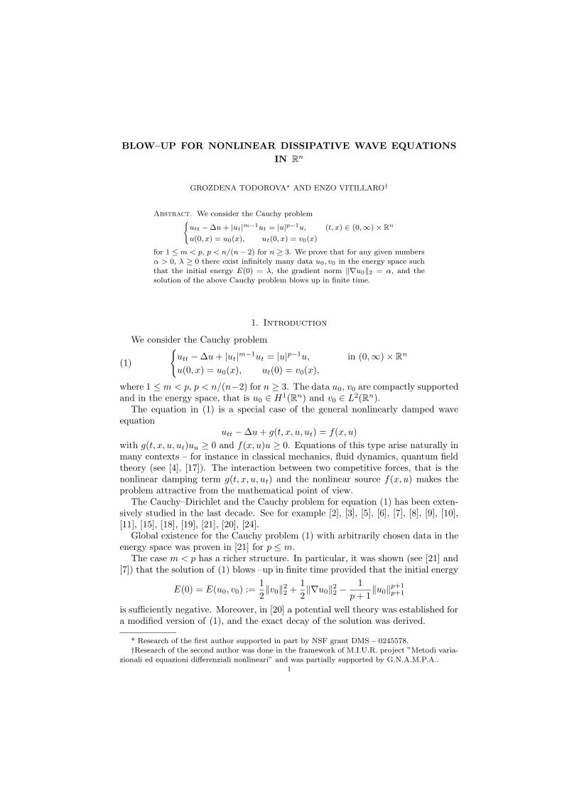
BLOW–UP FOR NONLINEAR DISSIPATIVE WAVE EQUATIONS

IN Rn

GROZDENA TODOROVA∗ AND ENZO VITILLARO†

Abstract. We consider the Cauchy problem{

utt − ∆u + |ut|m−1ut = |u|p−1u, (t, x) ∈ (0,∞) × Rn

u(0, x) = u0(x), ut(0, x) = v0(x)

for 1 ≤ m < p, p < n/(n− 2) for n ≥ 3. We prove that for any given numbers

α > 0, λ ≥ 0 there exist infinitely many data u0, v0 in the energy space such

that the initial energy E(0) = λ, the gradient norm ‖∇u0‖2 = α, and thesolution of the above Cauchy problem blows up in finite time.

1. Introduction

We consider the Cauchy problem

(1)

{utt − ∆u+ |ut|

m−1ut = |u|p−1u, in (0,∞) × Rn

u(0, x) = u0(x), ut(0) = v0(x),

where 1 ≤ m < p, p < n/(n−2) for n ≥ 3. The data u0, v0 are compactly supportedand in the energy space, that is u0 ∈ H1(Rn) and v0 ∈ L2(Rn).

The equation in (1) is a special case of the general nonlinearly damped waveequation

utt − ∆u+ g(t, x, u, ut) = f(x, u)

with g(t, x, u, ut)uu ≥ 0 and f(x, u)u ≥ 0. Equations of this type arise naturally inmany contexts – for instance in classical mechanics, fluid dynamics, quantum fieldtheory (see [4], [17]). The interaction between two competitive forces, that is thenonlinear damping term g(t, x, u, ut) and the nonlinear source f(x, u) makes theproblem attractive from the mathematical point of view.

The Cauchy–Dirichlet and the Cauchy problem for equation (1) has been exten-sively studied in the last decade. See for example [2], [3], [5], [6], [7], [8], [9], [10],[11], [15], [18], [19], [21], [20], [24].

Global existence for the Cauchy problem (1) with arbitrarily chosen data in theenergy space was proven in [21] for p ≤ m.

The case m < p has a richer structure. In particular, it was shown (see [21] and[7]) that the solution of (1) blows –up in finite time provided that the initial energy

E(0) = E(u0, v0) :=1

2‖v0‖

22 +

1

2‖∇u0‖

22 −

1

p+ 1‖u0‖

p+1p+1

is sufficiently negative. Moreover, in [20] a potential well theory was established fora modified version of (1), and the exact decay of the solution was derived.

* Research of the first author supported in part by NSF grant DMS – 0245578.

†Research of the second author was done in the framework of M.I.U.R. project ”Metodi varia-

zionali ed equazioni differenziali nonlineari” and was partially supported by G.N.A.M.P.A..1

2 G. TODOROVA AND E. VITILLARO

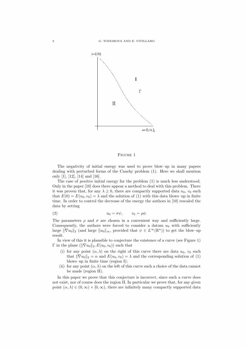
Figure 1

The negativity of initial energy was used to prove blow–up in many papersdealing with perturbed forms of the Cauchy problem (1). Here we shall mentiononly [1], [12], [14] and [16].

The case of positive initial energy for the problem (1) is much less understood.Only in the paper [10] does there appear a method to deal with this problem. Thereit was proven that, for any λ ≥ 0, there are compactly supported data u0, v0 suchthat E(0) = E(u0, v0) = λ and the solution of (1) with this data blows–up in finitetime. In order to control the decrease of the energy the authors in [10] rescaled thedata by setting

(2) u0 = σψ, v0 = ρφ.

The parameters ρ and σ are chosen in a convenient way and sufficiently large.Consequently, the authors were forced to consider a datum u0 with sufficientlylarge ‖∇u0‖2 (and large ‖u0‖∞, provided that ψ ∈ L∞(Rn)) to get the blow–upresult.

In view of this it is plausible to conjecture the existence of a curve (see Figure 1)Γ in the plane (‖∇u0‖2, E(u0, v0)) such that

(i) for any point (α, λ) on the right of this curve there are data u0, v0 suchthat ‖∇u0‖2 = α and E(u0, v0) = λ and the corresponding solution of (1)blows–up in finite time (region I);

(ii) for any point (α, λ) on the left of this curve such a choice of the data cannotbe made (region II).

In this paper we prove that this conjecture is incorrect, since such a curve doesnot exist, nor of course does the region II. In particular we prove that, for any givenpoint (α, λ) ∈ (0,∞) × [0,∞), there are infinitely many compactly supported data

BLOW–UP FOR NONLINEAR DISSIPATIVE WAVE EQUATIONS IN Rn 3

u0, v0 in the energy space such that

‖∇u0‖2 = α, E(u0, v0) = λ

and the solution blows–up in finite time (Theorem 2).We point out that for the Cauchy–Dirichlet problem associated with (1) an

analogous result is false. Indeed it is well known that for ‖∇u0‖2 and E(u0, v0)sufficiently small the solution of the Cauchy–Dirichlet problem is global, due to thepotential well theory (see [13]). On the contrary, the result in [10] is known (ina stronger form) for the Cauchy–Dirichlet problem, when the energy level is lowerthan the potential well level (see [11] and [24]).

Moreover, as a byproduct of the proof of our main result we get that, for n ≥ 3,we can have blow–up for conveniently chosen data u0 ∈ H1(Rn) ∩ L∞(Rn), v0 ∈L2(Rn) with arbitrarily small L∞ norm and positive fixed energy λ.

We recall that for any point in a small neighborhood of the origin in the plane(‖∇u0‖2, E(u0, v0)) there are data small enough (namely data with σ and ρ suf-ficiently small in (2)), such that the solution of (1) is global. For this result inthe case of linear damping (m = 1) and p > 1 + 2/n see [23]. The result fornonlinear damping and sufficiently large p will be presented in [22]. So, in theabove neighborhood we have two choices for the data: one that causes blow up andthe other that insures global existence. It is an interesting open problem whetherthis neighborhood is the only domain in the plane (‖∇u0‖2, E(u0, v0)) with thisproperty.

The technique we use is a natural development on the arguments of [10]. How-ever, some important differences arise. In particular, since we want to keep thenorm ‖∇u0‖2 fixed we cannot use the simple rescaling (2) of the data with σ → ∞.Instead we use a transformation which keeps ‖∇u0‖2 and E(u0, v0) fixed, but theprice for this is to raise the radius of the support of the data. As a consequence wecannot use the estimates in [10] because, roughly speaking, they are based on finitespeed of propagation while for our purpose we need to use “pure”– R

n estimates.In this way we “clean” the estimates in [10] from dependence on the support of thedata, or when we cannot avoid this dependence we take it into account explicitly. Afurther advantage of these estimates is that they may be adapted to other equationsfor which the finite speed of propagation property does not apply.

2. Preliminaries and statement of the main result

The following local existence and regularity result for the Cauchy problem (1)can be found in [21] (see also [2]).

Theorem 1. Let

1 ≤ m < p, p <n

n− 2for n ≥ 3.

Then, for any compactly supported data

u0 ∈ H1(Rn), v0 ∈ L2(Rn),

the Cauchy problem (1) has a unique solution

u(t, x) ∈ C([0, T );H1(Rn)),(3)

ut(t, x) ∈ C([0, T );L2(Rn)) ∩ Lm+1([0, T ) × Rn),(4)

provided T is small enough.


To state our main result we introduce the domain Dn in R2 defined by the

following inequalities

m(n− 2)(p+ 1)2 < 4(p+ n+ 1) if n ≥ 3,(5)

and

p[(n− 2)m2 + (n− 2)m+ 4] < −(n− 2)m2 + 3(n+ 2)m if n ≥ 2,(6)

or

p[(n− 2)m+ n] < −(n− 2)m+ 3n+ 4 if n ≥ 2.(7)

Namely

(8) Dn = {(p,m) ∈ (1,∞) × [1,∞) : (5) and (6) or (7) hold}.

Theorem 2. Let

(9) 1 ≤ m < p, p <n

n− 2for n ≥ 3,

and (p,m) ∈ Dn. Then, for any λ ≥ 0 and any α > 0 there are infinitely many 1

compactly supported data u0 ∈ H1(Rn) and v0 ∈ L2(Rn) such that

E(u0, v0) =1

2‖∇u0‖

22 +

1

2‖v0‖

22 −

1

p+ 1‖u0‖

p+1p+1 = λ,(10)

‖∇u0‖2 = α(11)

and the solution of the Cauchy problem (1) blows–up in finite time, i.e. there is

Tmax <∞ such that limt→T−

max

‖u(t)‖p+1 = ∞.

As a byproduct of the proof of Theorem 2 we have

Corollary 1. Let the assumptions of Theorem 2 hold and n ≥ 3. For any α > 0and λ ≥ 0 there are compactly supported data u0 ∈ H1(Rn) ∩ L∞(Rn) and v0 ∈L2(Rn), with ‖u0‖∞ arbitrarily small, such that (10)–(11) hold and the solution of

the Cauchy problem (1) blows–up in finite time.

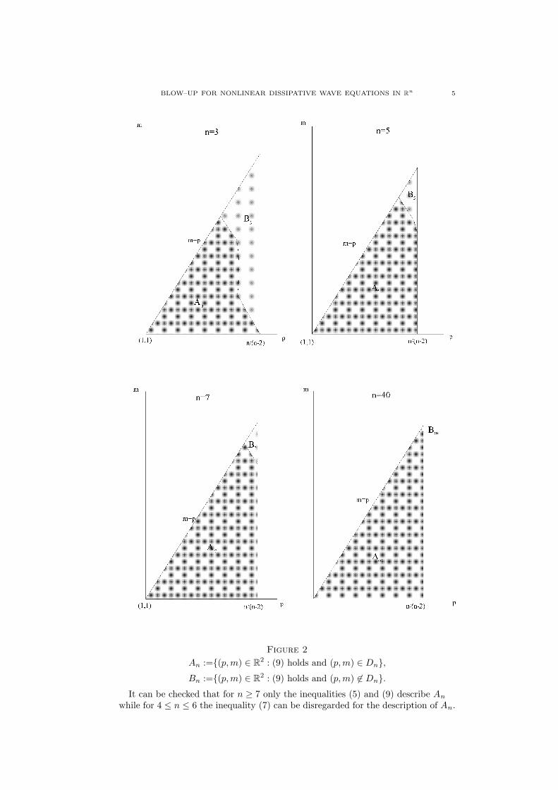
Remark 1. The technical condition (p,m) ∈ Dn cuts a small part Bn from thenatural set for the exponents of nonlinearities endowed by (9). How small is thiscut is illustrated in Figure 2. The figure shows that when the space dimension nincreases the set Bn becomes negligible. For n = 1 there is no cut at all, whichtogether with the behavior of Bn for large n, naturally brings the conjecture thatconditions (5)–(7) are method driven for all n ∈ N.

In the proof we shall use the well known Gagliardo–Nirenberg estimate. For thesake of completeness we recall it here.

Lemma 1 (Gagliardo–Nirenberg). Let 1 ≤ r < q ≤ ∞, and q ≥ 2. Then the

inequality

‖v‖q ≤ C‖∇v‖θ2‖v‖

1−θr , for v ∈ H1(Rn) ∩ Lr(Rn)

1actually a continuous branch


Figure 2

An :={(p,m) ∈ R2 : (9) holds and (p,m) ∈ Dn},

Bn :={(p,m) ∈ R2 : (9) holds and (p,m) 6∈ Dn}.

It can be checked that for n ≥ 7 only the inequalities (5) and (9) describe An

while for 4 ≤ n ≤ 6 the inequality (7) can be disregarded for the description of An.


holds with some positive constant C = C(r, q, n) and

(12) θ =

1

r−

1

q1

n+

1

r−

1

2

,

provided that 0 < θ < 1.

3. Proofs

Proof of Theorem 2. Let λ ≥ 0 and α > 0 be fixed, and let u0 and v0 be data to bechosen in the sequel, u0 ∈ H1(Rn), v0 ∈ L2(Rn), with support contained in a ballBL := {x ∈ R

n : |x| ≤ L}, L > 0, such that E(u0, v0) = λ and ‖∇u0‖2 = α. Let ube the corresponding solution of (1).

In the sequel C will indicate different positive constants, dependent only on p,m and n, but independent of L and u0, v0.

The energy of the solution u is

(13) E(t) =1

2‖ut(t)‖

22 +

1

2‖∇u(t)‖2

2 −1

p+ 1‖u(t)‖p+1

p+1.

We recall one of the blow–up results in [21], [7]. There is a critical level of theenergy Ecr, with

(14) −max{1, CL−C} ≤ Ecr ≤ 0,

such that if

(15) E(t) < Ecr

for some t > 0 then the solution of the Cauchy problem (1) blows–up in finitetime.2

By the energy identity we have

(16) E(0) − E(t) =

∫ t

0

‖ut‖m+1m+1.

Then the blow–up sufficient condition (15) can be rewritten as

(17)

∫ t

0

‖ut‖m+1m+1 > E(0) − Ecr,

for some t > 0.The idea is to control the dissipation

∫ t

0‖ut‖

m+1m+1 of the energy E(t) in order to

assure that the energy E(t) overpasses the critical level Ecr for conveniently chosendata u0 , v0 with prescribed energy E(0) and ‖∇u0‖. All estimates we derive tocontrol this dissipation hold locally, i.e. for a small time interval. A delicate pointis to show that the data can be chosen such that in this small time interval thereis a time t such that the blow–up condition (17) holds.

For contradiction we assume that the solution u is global, so that

(18) E(t) = E(t) −1

p+ 1‖u‖p+1

p+1 ≥ Ecr, for all t ≥ 0,

2Let us notice that the condition∫

Rnu0v0 ≥ 0 mentioned in [21] can be avoided. Indeed, the

requirement F (0) ≥ 0 at [21, p. 898 – Case 2], which leads to the condition mentioned above, can

be skipped by taking ε so small that ε|F (0)| ≤ LAH(0)1−α/2.


where

(19) E(t) :=1

2‖ut‖

22 +

1

2‖∇u‖2

2.

Namely,

(20) ‖u(t)‖p+1 ≤ (p+ 1)1/(p+1)[E(t) − Ecr]1/(p+1) for all t ≥ 0.

By using the Holder inequality and the finite speed of propagation of u, we have

(21) ‖ut‖m+1m+1 ≥ C(L+ t)−n(m−1)/2‖ut‖

m+12 .

To estimate ‖ut‖m+12 from below we use the inequality

(22) ‖g‖2 ≥ ‖g‖H−1(Rn), for all g ∈ L2(Rn).

Indeed H−1(Rn) (in the sequel simply denoted by H−1) is a natural space for waveequations with data in the energy space.

A main tool in the proof is to decompose the solution u to the sum of the solutionof the free wave equation with the same data and a remainder term, i.e.

(23) u = w + v,

where

(24)

{wtt − ∆w = 0, in (0,∞) × R

n,

w(0, x) = u0(x), wt(0, x) = v0(x), in Rn.

The remainder term v is a solution of the Cauchy problem

(25)

{vtt − ∆v = F (t, x), in (0,∞) × R

n,

v(0, x) = 0, vt(0, x) = 0, in Rn,

where

(26) F (t, x) := |u|p−1u− |ut|m−1ut.

The main difference with the corresponding proof in [10] is the following. In viewof our further choice of the data in which the radius of the support L will not be

fixed, we need the estimates to be either independent on L or, if that is not possible,to control carefully the L dependence. Actually we can avoid any L–dependenceeverywhere except in the next estimate.

By using the decomposition (23) together with (21) and (22) we have

(27)‖ut‖

m+1m+1 ≥C(L+ t)−n(m−1)/2‖ut‖

m+1H−1

≥C(L+ t)−n(m−1)/2(‖wt‖

m+1H−1 − ‖vt‖

m+1H−1

).

By (27) we need estimates of the term ‖wt‖m+1H−1 from below and ‖vt‖

m+1H−1 from

above which hold for a small time interval.To estimate ‖wt‖

m+1H−1 from below we use the fundamental solution of the free

wave equation (24)

(28) w(t, ξ) = cos(t|ξ|)u0(ξ) +sin(t|ξ|)

|ξ|v0(ξ)


where w is the Fourier transform of w. Then the arguments of [10] yield that theinequality [10, 3.16] holds. In order to avoid the L–dependence in the estimate for‖wt‖

m+1H−1 , we can rewrite this inequality in the form

|wt(t, ξ)|2 ≥

1

2|v0|

2 − t2|ξ|2(|∇u0(ξ)|

2 + |v0|2).

This directly implies

1

2‖v0‖

2H−1 ≤ ‖wt‖

2H−1 + 2t2E(0),

which leads to the final L–independent estimate for ‖wt‖m+1H−1

(29) ‖wt‖m+1H−1 ≥ C

(‖v0‖

m+1H−1 − Ctm+1E(m+1)/2(0)

).

The estimate of the term ‖vt‖m+1H−1 from above is much more delicate. Taking the

H−1 scalar product of both sides of (25) by vt, using the identity

−(∆v, vt)H−1 =1

2

d

dt‖∇v‖2

H−1 ,

and integrating on [0, t] we obtain

1

2‖vt‖

2H−1 +

1

2‖∇v‖2

H−1 ≤

∫ t

0

‖F (·, t)‖H−1‖vt‖H−1 .

In the above we use that the initial data in (25) are zero. Applying a Gronwalltype inequality we obtain

(30) ‖vt‖H−1 ≤

∫ t

0

‖F (·, η)‖H−1 dη.

Using (26) we have

(31) ‖F (·, η)‖H−1 ≤ ‖|u|p−1u‖H−1 + ‖|ut|m−1ut‖H−1 .

The Sobolev embedding states

(32) ‖g‖H−1 ≤ C(l, n)‖g‖l, for all g ∈ Ll(Rn),

where C(l, n) is a positive constant, for any 1 < l ≤ 2 and l ≥ 2n/(n+ 2). We use(32) to estimate the first and the second term on the right–hand side of (31), withl = (p + 1)/p and l = (m + 1)/m respectively. For this choice of l the inequality(32) holds because l ≥ 2n/(n+ 2) since 1 ≤ m < p < n/(n− 2). Then we have

(33)‖F (·, η)‖H−1 ≤C

(‖u‖p

p+1 + ‖ut‖mm+1

)

≤C[(E(t) − Ecr)

p/(p+1) + ‖ut‖mm+1

],

where we used the estimate (20).The estimates (30) and (33) together with the Holder inequality with respect to

t imply

‖vt‖H−1 ≤ C

[∫ t

0

(E(η) − Ecr)p/(p+1) dη + t1/(m+1)

(∫ t

0

‖ut‖m+1m+1

)m/(m+1)].

By (16) and (18) we come to

(34) ‖vt‖H−1 ≤ C

[∫ t

0

(E(η) − Ecr)p/(p+1) dη + t1/(m+1) (E(0) − Ecr)

m/(m+1)

].


The advantage of this estimate compared with [10, 3.22] is that (34) is supportindependent while [10, 3.22] is not.

It is clear now that we need a local in time estimate for E(t) from above. Notethat, by (19) and the energy identity,

(35) E′(t) = −‖ut‖m+1m+1 +

∫

Rn

|u|p−1uut.

From (35) we shall derive an ordinary differential inequality of the type(E(t) + C

)′

≤ C1

(E(t) + C

)α

.

This can be done in two different ways and the best choice between them relies onminimizing the exponent α. This maximizes the time interval for which the finalestimate applies. This optimal choice depends on the exponents p and m of thenonlinearities and on the dimension of the space n.

First estimate of E′(t). By using Young’s inequality from (35) we get

(36)E′(t) ≤− ‖ut‖

m+1m+1 +

m

m+ 1

∫

Rn

|u|p(m+1)/m +1

m+ 1

∫

Rn

|ut|m+1

≤m

m+ 1‖u‖

p(m+1)/mp(m+1)/m.

To estimate the right–hand side of (36) we use the Gagliardo – Nirenberg estimate(Lemma 1) with

q =p(m+ 1)

mand r = p+ 1.

Thus we have

(37) E′(t) ≤ C(‖∇u‖θ1

2 ‖u‖1−θ1

p+1

)p(m+1)/m

,

where

θ1 :=

1

p+ 1−

m

p(m+ 1)1

n+

1

p+ 1−

1

2

.

An elementary calculation shows that

(38) θ1 =2n(p−m)

p(m+ 1)[2n− (n− 2)(p+ 1)],

which gives 0 < θ1 < 1 since 1 < m < p and p < n/(n− 2) (for n ≥ 3).By using estimates (19), (20) and (37) we obtain the inequality

E′(t) ≤ C

[Eθ1/2(t)

(E(t) − Ecr

)(1−θ1)/(p+1)]p(m+1)/m

.

Since Ecr ≤ 0, it follows that

(39) E′(t) ≤ C(E(t) − Ecr

)γ1

,

where

(40) γ1 =p(m+ 1)

m

(θ12

+1 − θ1p+ 1

).


Using (38) and (40), elementary calculations show that

(41) γ1 = 1 +2(p−m)

m[2n− (n− 2)(p+ 1)]> 1.

This concludes our first estimate of E′(t).

Second estimate of E′(t). Neglecting the first term in the right–hand side of (35)and using Schwartz inequality, we obtain

(42) E′(t) ≤

∫

Rn

|u|p−1uut ≤

∫

Rn

|u|p|ut| ≤ ‖ut‖2‖u‖p2p.

We apply the Gagliardo–Nirenberg inequality (Lemma 1), with

q = 2p and r = p+ 1,

to get

(43) ‖u‖2p ≤ C‖∇u‖θ2

2 ‖u‖1−θ2

p+1 ,

where

θ2 =

1

p+ 1−

1

2p1

n+

1

p+ 1−

1

2

.

An elementary calculation shows that

(44) θ2 =n(p− 1)

p[2n− (n− 2)(p+ 1)],

and 0 < θ2 < 1 since 1 < m < p and p < n/(n − 2) (for n ≥ 3). Then, sinceEcr ≤ 0, by (19), (20) and (43) we have

(45)‖u‖2p ≤CEθ2/2(t)

[E(t) − Ecr

](1 − θ2)/(p+ 1)

≤C(E(t) − Ecr

)(1 − θ2)/(p+ 1) + θ2/2.

By using the estimates (19), (45) and the fact that Ecr ≤ 0 we can rewrite (42) inthe following form

(46) E′(t) ≤ C(E(t) − Ecr

)γ2

,

where

(47) γ2 =1

2+ p

(θ22

+1 − θ2p+ 1

).

Moreover, elementary calculations show that

(48) γ2 = 1 +p− 1

2n− (n− 2)(p+ 1)> 1,

where we used (44) as well. This concludes our second estimate of E′(t).

To choose between estimates (39) and (46) we minimize the exponent of(E(t) − Ecr

).

We set

(49) γ0 := min{γ1, γ2}.


By (41) and (48) it is clear that γ0 > 1. So we can rewrite (39) and (46) as

(50) (E − Ecr)′(t) = E′(t) ≤ C(E(t) − Ecr)

γ0 .

Integrating (50) we get

(51) (E − Ecr)1−γ0(t) ≥ (E − Ecr)

1−γ0(0) − (γ0 − 1)Ct.

For t small enough, namely

(52) t ≤ T1 := C(E(0) − Ecr

)1−γ0

,

by (51) we have

(53) E(t) − Ecr ≤ 2(E(0) − Ecr).

In the last step we used that γ0 > 1. The estimate (53) is the final estimate for

E(t), which applies for t given by (52).Turning back to the main estimate (34) and using the inequality (53), we obtain

‖vt‖H−1 ≤ C[t(E(0) − Ecr)

p/(p+1) + t1/(m+1) (E(0) − Ecr)m/(m+1)

],

as long as t ≤ T1. The above estimate yields

(54) ‖vt‖m+1H−1 ≤ C

[tm+1(E(0) − Ecr)

p(m+1)/(p+1) + t (E(0) − Ecr)m

].

This is our final estimate of ‖vt‖m+1H−1 , which applies for t ≤ T1.

This estimate together with (29) gives us the possibility to rewrite the inequality(27) in the form

(55) ‖ut‖m+1m+1 ≥ C(L+ t)−n(m−1)/2

[‖v0‖

m+1H−1 − Ctm+1E(m+1)/2(0)

−Ctm+1(E(0) − Ecr)p(m+1)/(p+1) − Ct (E(0) − Ecr)

m],

as long as t ≤ T1. We simplify the inequality (55) in the following way

(56) ‖ut‖m+1m+1 ≥ CL−n(m−1)/2

[‖v0‖

m+1H−1 − Ctm+1(E(0) −Ecr)

p(m+1)/(p+1)

−Ct (E(0) −Ecr)m

] ,

as long as t ≤ min{L, T1}; here it was taken into account that E(0) ≤ E(0) − Ecr,

p(m + 1)/(p + 1) > (m + 1)/2 together with the assumption E(0) > 1. The lastassumption is natural since in the sequel we shall choose data with sufficiently large

E(0). Integrating (56) on [0, t], t ≤ min{L, T1}, we get

(57)

∫ t

0

‖ut‖m+1m+1 ≥ CL−n(m−1)/2t

[‖v0‖

m+1H−1 − Ctm+1(E(0) − Ecr)

p(m+1)/(p+1)


] .

We recall that the inequality (17) assures the blow–up of the solution of (1). Takinginto account the estimate (57), we have to prove that there exist data such that

(58)

∫ t

0

‖ut‖m+1m+1 ≥CL−n(m−1)/2t

[‖v0‖

m+1H−1 − Ctm+1(E(0) − Ecr)

p(m+1)/(p+1)


]≥ E(0) − Ecr

for some t ≤ min{L, T1}.


Now we start with the choice of the data u0 and v0. Let ψ ∈ H1(Rn) andφ ∈ L2(Rn) be fixed, with supp ψ, supp φ ⊂ B1, ‖∇ψ‖2 = α. For the sake ofsimplicity we normalize ‖φ‖H−1 = 1.

Consider a transformation of φ and ψ of the type

(59) u0(x) = µ1−n/2ψ(x/µ), and v0(x) = βφ(x/µ),

where β > 0 and µ ≥ 1 will be chosen in the sequel. This transformation preserves‖∇ψ‖2 and transforms the energy into

(60) E(0) =1

2‖φ‖2

2β2µn +

1

2α2 −

1

p+ 1µ[2n−(n−2)(p+1)]/2‖ψ‖p+1

p+1.

Since we need data with prescribed energy λ, the two parameters µ and β arerelated by

(61)1

2‖φ‖2

2β2µn +

1

2α2 −

1

p+ 1µ[2n−(n−2)(p+1)]/2‖ψ‖p+1

p+1 = λ.

For µ sufficiently large, namely for µ ≥ µ(p, n, α, λ, ‖ψ‖p+1), the above equation(61) has a (unique) positive solution β = β(µ). This argument, together with thetransformation (59), reduces the choice of the data to a convenient choice for µ,such that the inequality (58) holds for a suitably chosen t = t1 ≤ min{L, T1}.

Let us note that by the transformation (59) we have

(62) supp u0 ⊂ Bµ, supp v0 ⊂ B1 ⊂ Bµ, so that L = µ, .

As a consequence of (61) we have

(63) β ∼ Kµ−(n−2)(p+1)/4, as µ→ ∞,

where K = K(ψ, φ, p, α, λ) > 0. This shows that βµn/2 → ∞ as µ → ∞ sincep < n/(n− 2). Then

(64) E(0) =1

2β2µn‖φ‖2

2 +1

2α2 → ∞ as µ→ ∞.

Now we can point out one of the difficulty in the proof. First L = µ must belarge enough in order that equation (61) has a solution β, while L large yields thatthe factor L−n(m−1)/2 is small in (58). Moreover, the identity (52) and the limit(64) imply that T1 → 0 as µ → ∞, together with any t ≤ max{µ, T1} for which(58) holds. So, as µ→ ∞, the factor CL−n(m−1)/2t in (58) goes to zero at least asfast as µ−n(m−1)/2T1, regardless of the value t ≤ {µ, T1}. This forces the remainderterm in (58) (namely the term inside the brackets) to compensate this fast decrease.This is the origin of the technical assumption (p,m) ∈ Dn.

Simple calculations show that

(65) ‖v0‖H−1 ∼ Cβµn/2 → ∞ as µ→ ∞.

Now, due to (14) and (62) we have E(0) − Ecr = λ − Ecr ≤ λ + 1 for µ largeenough. This gives us a possibility to neglect the last term in the first inequality of(58) and to rewrite (58) as follows

(66)

∫ t

0

‖ut‖m+1m+1 ≥Cµ−n(m−1)/2t

[‖v0‖

m+1H−1 − Ctm+1(E(0) − Ecr)

p(m+1)/(p+1)]

≥E(0) − Ecr

for some t ≤ min{T1, µ}, and for C = C(p,m, n, α, λ, φ, ψ) > 0.


For the sake of positivity of the right hand side of the first inequality in (66), wechoose t1 in the form

(67) t1 = ‖v0‖H−1

(E(0) − Ecr

)−ν

where ν > 0 has to be determined in the sequel. Since the estimate (66) is satisfiedfor t ≤ min{T1, µ}, we require that t1 ≤ T1 for µ sufficiently large. Using theestimate

‖v0‖H−1 ≤ ‖v0‖2 ≤ E1/2(0),

together with (52), (64) and (67) we get

(68) ν > γ0 −1

2.

For µ large enough we have T1 ≤ µ (see (52) and (64)) so the value of t1 from (67)satisfies our requirements. We put t = t1 in (66) and get

(69)

∫ t1

0

‖ut‖m+1m+1 ≥ Cµ−n(m−1)/2‖v0‖

m+2H−1

(E(0) − Ecr

)−ν

×[1 − C(E(0) − Ecr)

(m+1)[p/(p+1)−ν]].

From the asymptotic behavior of E(0) as µ→ ∞, and for the sake of positivityof the right and side of (69), we require that

(70) 1 − C(E(0) − Ecr)(m+1)(p/(p+1)−ν) ≥ C > 0.

The last inequality holds provided that

(71) ν >p

p+ 1.

Then, for ν satisfying (68) and (71), we can simplify (66) by using (69) togetherwith (70) in the following way

(72)

∫ t1

0

‖ut‖m+1m+1 ≥ Cµ−n(m−1)/2‖v0‖

m+2H−1

(E(0) − Ecr

)−ν

≥ E(0) − Ecr

for µ large enough. Taking into account the asymptotic behavior of ‖v0‖H−1 and

E(0) together with (63) as µ → ∞ the estimate (72) holds for µ large enoughprovided that

(73) −n(m− 1)

2+

2n− (n− 2)(p+ 1)

4(m+ 2) −

2n− (n− 2)(p+ 1)

2ν > 0.

Solving the system (68), (71) and (73) leads to the restriction on m and p andthe space dimension n which is expressed by the condition (p,m) ∈ Dn (see (8)).

The existence of a solution µ of the elementary inequalities (68), (71) and (73)bring us to a contradiction with the assumption that the solution is global. This,together with the continuation principle (see [17]) implies finite time blow–up ofthe solution. Since this is true for µ large enough there is a continuous branchµ → (u0(µ), v0(µ)) of data satisfying (10) and (11) for which the solution of (1)blows up. �


Proof of Corollary 1. We choose ψ ∈ H1(Rn) ∩ L∞(Rn). Then, from the transfor-mation (59) we get

(74) ‖u0‖∞ = µ1−n/2‖ψ‖∞.

The same argument as in the proof of Theorem 2 concludes the proof of the Corol-lary. �

4. Acknowledgment

The second author thanks the Department of Mathematics, University of Ten-nessee, were the work was done, for the kind hospitality.

References

[1] V. Barbu, I. Lasiecka, and M.A. Rammaha, On nonlinear wave equations with degenerate

damping and source terms, preprint.

[2] V. Georgiev and G. Todorova, Existence of a solution of the wave equation with nonlinear

damping and source terms, J. Differential Equations 109 (1994), 295–308.

[3] R. Ikehata, Some remarks on the wave equations with nonlinear damping and source terms,

Nonlinear Anal. 27 (1996), no. 10, 1165–1175.[4] K. Jorgens, Das Anfangswertproblem im Grossen fur eine Klasse nichtlinearer Wellengle-

ichungen, Math. Z. 77 (1961), 295–308.[5] H. A. Levine, Instability and nonexistence of global solutions to nonlinear wave equations of

the form Putt = −Au + F(u), Trans. Amer. Math. Soc. 192 (1974), 1–21.

[6] , Some additional remarks on the nonexistence of global solutions to nonlinear wave

equations, SIAM J. Math. Anal. 5 (1974), 138–146.

[7] H. A. Levine, S. R. Park, and J. Serrin, Global existence and global nonexistence of solutions

of the cauchy problem for a nonlinearly damped wave equation, J. Math. Anal. Appl. 228

(1998), 181–205.

[8] H. A. Levine, P. Pucci, and J. Serrin, Some remarks on global nonexistence for nonau-

tonomous abstract evolution equations, Harmonic Analysis and Nonlinear Differential Equa-

tions (M. L. Lapidus, L. H. Harper, and A. J. Rumbos, eds.), Contemp. Math., 208, AmericanMathematical Society, 1997, pp. 253–263.

[9] H. A. Levine and J. Serrin, Global nonexistence theorems for quasilinear evolutions equations

with dissipation, Arch. Rational Mech. Anal. 137 (1997), 341–361.[10] H. A. Levine and G. Todorova, Blow up of solutions of the Cauchy problem for a wave

equation with nonlinear damping and source terms and positive initial energy, Proc. Amer.Math. Soc. 129 (2001), no. 3, 693–805.

[11] M. Ohta, Remark on blow–up of solutions for nonlinear evolution equations of second order,

Adv. in Math. Sc. and Appl. 8 (1998), 901–910.[12] K. Ono, On global solutions and blow–up solutions of nonlinear Kirchoff string with nonlinear

dissipations, J. Math. Anal. Appl. 216 (1997), 321–342.[13] L. E. Payne and D. H. Sattinger, Saddle points and instability of nonlinear hyperbolic equa-

tions, Israel J. Math. 22 (1975), 273–303.[14] D. R. Pitts and M.A. Rammaha, Global existence and non-existence theorems for nonlinear

wave equations, Indiana Univ. Math. J. 51 (2002), no. 6, 1479–1509.

[15] P. Pucci and J. Serrin, Global nonexistence for abstract evolution equations with positive

initial energy, J. Differential Equations 150 (1998), no. 1, 203–214.

[16] M. A. Rammaha and T. A. Strei, Global existence and nonexistence for nonlinear wave

equations with damping and source terms, Trans. Amer. Math. Soc. 354 (2002), no. 9, 3621–

3637 (electronic).

[17] I. Segal, Nonlinear semigroups, Ann. of Math. 78 (1963), 339–364.[18] J. Serrin, G. Todorova, and E. Vitillaro, Existence for a nonlinear wave equation with non-

linear damping and source terms, Differential Integral Equation 16 (2003), no. 1, 13–50.[19] W. A. Strauss, Nonlinear wave equations, Regional conference series in mathematics, vol. 73,

Amer.Math.Soc., Providence, R.I., 1989.


[20] G. Todorova, Stable and unstable sets for the Cauchy problem for a nonlinear wave equation

with nonlinear damping and source terms, J. Math. Anal. Appl. 239 (1999), 213–226.

[21] , Cauchy problems for a nonlinear wave equations with nonlinear damping and source

terms, Nonlinear Anal. 41 (2000), 891–905.

[22] G. Todorova and B. Yordanov, Critical exponent for a nonlinear wave equation with nonlinear

damping term, to appear.[23] , Critical exponent for a nonlinear wave equation with damping, J. Differential Equa-

tions 174 (2001), no. 2, 464–489.

[24] E. Vitillaro, Global nonexistence theorems for a class of evolution equations with dissipation

and application, Arch. Rational Mech. Anal. 149 (1999), 155–182.

(G. Todorova) Department of Mathematics, The University of Tennessee, Knoxville,

TN 37996 U.S.A.

E-mail address: [email protected]

(E. Vitillaro) Dipartimento di Matematica e Informatica, Universita di Perugia Via

Vanvitelli,1 06123 Perugia ITALY

E-mail address: [email protected]

Blow-up for nonlinear dissipative wave equations i

Documents

Transcript of Blow-up for nonlinear dissipative wave equations i