
Bayesian subset simulation - arXiv · 2017-04-25 · BAYESIANSUBSETSIMULATION 3 In this article we...
35
Bayesian subset simulation * Julien Bect † , Ling Li ‡ , and Emmanuel Vazquez † Abstract. We consider the problem of estimating a probability of failure α, defined as the volume of the excursion set of a function f : X ⊆ R d → R above a given threshold, under a given probability measure on X. In this article, we combine the popular subset simulation algorithm (Au and Beck, Probab. Eng. Mech. 2001) and our sequential Bayesian approach for the estimation of a probability of failure (Bect, Ginsbourger, Li, Picheny and Vazquez, Stat. Comput. 2012). This makes it possible to estimate α when the number of evaluations of f is very limited and α is very small. The resulting algorithm is called Bayesian subset simulation (BSS). A key idea, as in the subset simulation algorithm, is to estimate the probabilities of a sequence of excursion sets of f above intermediate thresholds, using a sequential Monte Carlo (SMC) approach. A Gaussian process prior on f is used to define the sequence of densities targeted by the SMC algorithm, and drive the selection of evaluation points of f to estimate the intermediate probabilities. Adaptive procedures are proposed to determine the intermediate thresholds and the number of evaluations to be carried out at each stage of the algorithm. Numerical experiments illustrate that BSS achieves significant savings in the number of function evaluations with respect to other Monte Carlo approaches. Key words. Probability of failure, Computer experiments, Sequential design, Gaussian process, Stepwise uncertainty reduction Sequential Monte Carlo AMS subject classifications. 62L05, 62K99, 62P30 1. Introduction. Probabilistic reliability analysis has become over the last thirty years an essential part of the engineer’s toolbox (see, e.g., [19, 44, 47]). One of the central problems in probabilistic reliability analysis is the computation of the probability of failure (1) α = Z X 1 f ≤0 dP X of a system (or a component in a multicomponent system; see, e.g., [48], where P X is a probability measure over some measurable space (X, B) representing all possible sources of uncertainty acting on the system—both epistemic and aleatory—and f : X → R is the so-called limit-state function, such that f takes positive values when the system behaves reliably, and negative values when the system behaves unreliably, or fails. It is assumed in this article that X is a subset of R d —in other words, we consider reliability problems where all uncertain factors can be described as a d-dimensional random vector. Numerous * This research was partially funded by the French Fond Unique Interministériel (FUI 7) in the context of the CSDL (Complex Systems Design Lab) project. Parts of this work were previously published in the proceedings of the PSAM 11 & ESREL 12 conference [41] and in the PhD thesis of the second author [40]. † Laboratoire des Signaux et Systèmes, CentraleSupélec, CNRS, Univ. Paris-Sud, Université Paris-Saclay. 3 rue Joliot-Curie, 92192 Gif-sur-Yvette, France. Email: fi[email protected] ‡ Email: [email protected]. Present address: Schlumberger Gould Research Center, Cambridge, UK. 1 arXiv:1601.02557v3 [stat.CO] 24 Apr 2017
Transcript of Bayesian subset simulation - arXiv · 2017-04-25 · BAYESIANSUBSETSIMULATION 3 In this article we...
Bayesian subset simulation∗
Julien Bect† , Ling Li‡ , and Emmanuel Vazquez†
Abstract. We consider the problem of estimating a probability of failure α, defined as the volume of theexcursion set of a function f : X ⊆ Rd → R above a given threshold, under a given probabilitymeasure onX. In this article, we combine the popular subset simulation algorithm (Au and Beck,Probab. Eng. Mech. 2001) and our sequential Bayesian approach for the estimation of a probabilityof failure (Bect, Ginsbourger, Li, Picheny and Vazquez, Stat. Comput. 2012). This makes itpossible to estimate α when the number of evaluations of f is very limited and α is very small.The resulting algorithm is called Bayesian subset simulation (BSS). A key idea, as in the subsetsimulation algorithm, is to estimate the probabilities of a sequence of excursion sets of f aboveintermediate thresholds, using a sequential Monte Carlo (SMC) approach. A Gaussian processprior on f is used to define the sequence of densities targeted by the SMC algorithm, and drive theselection of evaluation points of f to estimate the intermediate probabilities. Adaptive proceduresare proposed to determine the intermediate thresholds and the number of evaluations to be carriedout at each stage of the algorithm. Numerical experiments illustrate that BSS achieves significantsavings in the number of function evaluations with respect to other Monte Carlo approaches.
Key words. Probability of failure, Computer experiments, Sequential design, Gaussian process, Stepwiseuncertainty reduction Sequential Monte Carlo
AMS subject classifications. 62L05, 62K99, 62P30
1. Introduction. Probabilistic reliability analysis has become over the last thirty yearsan essential part of the engineer’s toolbox (see, e.g., [19, 44, 47]). One of the centralproblems in probabilistic reliability analysis is the computation of the probability of failure
(1) α =
∫X
1f≤0 dPX
of a system (or a component in a multicomponent system; see, e.g., [48], where PX is aprobability measure over some measurable space (X,B) representing all possible sourcesof uncertainty acting on the system—both epistemic and aleatory—and f : X → R is theso-called limit-state function, such that f takes positive values when the system behavesreliably, and negative values when the system behaves unreliably, or fails. It is assumedin this article that X is a subset of Rd—in other words, we consider reliability problemswhere all uncertain factors can be described as a d-dimensional random vector. Numerous
∗This research was partially funded by the French Fond Unique Interministériel (FUI 7) in the context of theCSDL (Complex Systems Design Lab) project. Parts of this work were previously published in the proceedingsof the PSAM 11 & ESREL 12 conference [41] and in the PhD thesis of the second author [40].†Laboratoire des Signaux et Systèmes, CentraleSupélec, CNRS, Univ. Paris-Sud, Université Paris-Saclay.
3 rue Joliot-Curie, 92192 Gif-sur-Yvette, France. Email: [email protected]‡Email: [email protected]. Present address: Schlumberger Gould Research Center, Cambridge, UK.
1
arX
iv:1
601.
0255
7v3
[st
at.C
O]
24
Apr
201
7
2 JULIEN BECT, LING LI AND EMMANUEL VAZQUEZ
examples of applications that fall into this category can be found in the literature (see, forinstance, [5, 18, 34, 39, 54, 55]).
Two major difficulties usually preclude a brute-force Monte Carlo (MC) approach, thatis, using the estimator
αMC =1
m
m∑i=1
1f(Xi)≤0 , Xii.i.d∼ PX ,
which requires m evaluations of f . First, the evaluation of f for a given x ∈ X often relieson one or several complex computer programs (e.g., partial differential equation solvers)that take a long time to run. Second, in many applications, the failure region Γ = {x ∈X | f(x) ≤ 0} is a rare event under the probability PX; that is, the probability of failureα = PX(Γ) is small. When α is small, the standard deviation of αMC is approximately√α/m. To estimate α by MC with a standard deviation of 0.1α thus requires approximately
100/α evaluations of f . As an example, with α = 10−3 and 10 minutes per evaluation, thismeans almost two years of computation time.
The first issue—designing efficient algorithms to estimate α in the case of an expensive-to-evaluate limit-state function—can be seen as a problem of design and analysis of com-puter experiments (see, e.g., [50]), bearing some similarities to the problem of global op-timization (see [53] and references therein). Several sequential design strategies based onGaussian process models have been proposed in the literature, and spectacular evaluationsavings have been demonstrated on various examples with moderately small α (typically,10−2 or 10−3); see [6] for a review of fully sequential strategies and [3, 27] for examplesof two-stage strategies. The closely related problem of quantile estimation has also beeninvestigated along similar lines [1, 13, 46].
A key idea to address the second issue—i.e., to estimate a small probability of failure—is to consider a decreasing sequence of events Γ1 ⊃ Γ2 ⊃ · · · ⊃ ΓT = Γ such that theconditional probabilities PX (Γt | Γt−1) are reasonably large, and therefore easier to esti-mate than α itself. Then, sequential Monte Carlo simulations [21] can be used to produceestimates pt of the conditional probabilities PX (Γt | Γt−1), leading to a product-form esti-mate
∏Tt=1 pt for α. This idea, called subset simulation, was first proposed in [2] for the
simulation of rare events in structural reliability analysis1, but actually goes back to themuch older importance splitting (or multilevel splitting) technique used for the simulationof rare events in Markovian models (see, e.g., [36] and references therein). Subset simu-lation has since then become one of the most popular techniques for the computation ofsmall probabilities of failure, and the theoretical properties of several (most of the timesidealized) variants of the algorithm have recently been investigated by several authors (see,e.g., [11, 17]). However, because of the direct use of a Monte Carlo estimator for pt at eachstage t, the subset simulation algorithm is not applicable when f is expensive to evaluate.
1A very similar algorithm had in fact been proposed earlier by [23], but for a quite different purpose(estimating the probability of a rare event under the bootstrap distribution).
BAYESIAN SUBSET SIMULATION 3
In this article we propose a new algorithm, called Bayesian subset simulation (BSS),which tackles both issues at once using ideas from the sequential design of computer ex-periments and from the literature on sequential Monte Carlo methods. Section 2 reviewsthe subset simulation algorithm from the point of view of sequential Monte Carlo (SMC)techniques to prepare the ground for the introduction of our new algorithm. Section 3describes the algorithm itself and Section 4 presents numerical results. Finally, Section 5concludes the article with a discussion.
2. Subset simulation: a sequential Monte Carlo algorithm. This section recalls themain ideas of the classical subset simulation algorithm [2], which, although not originallypresented as such, can be seen as a sequential Monte Carlo sampler [17, 21].
2.1. Idealized subset simulation (with fixed levels and IID sampling). We con-sider the problem of estimating the probability α of a rare event Γ of the form Γ ={x ∈ X : f(x) > u}, where u ∈ R and f : X → R, using pointwise evaluations of f . Notethat the limit-state function (see Section 1) can be defined as x 7→ u− f(x) with our nota-tions. Assuming, for the sake of simplicity, that PX has a probability density function πXwith respect to Lebesgue’s measure, we have
α =
∫X
1f(x)>u πX(x) dx .
The key idea of the subset simulation algorithm is to introduce an increasing (finite)sequence of thresholds −∞ = u0 < u1 < u2 · · · < uT = u, which determine a correspondingdecreasing sequence of subsets:
X = Γ0 ⊃ Γ1 ⊃ · · · ⊃ ΓT = Γ, Γt := {x ∈ X : f(x) > ut} ,
of the input space X. Let αt = PX (Γt). The decreasing sequence (αt)0≤t≤T obeys therecurrence formula
(2) αt+1 = αt PX (Γt+1 | Γt) = αt
∫1Γt+1(x) qt(x) dx,
where qt stands for the truncated density
(3) qt(x) =1Γt(x)πX(x)∫1Γt(y)πX(y) dy
.
The small probability α = αT can thus be rewritten as a product of conditional probabilities,which are larger (and therefore easier to estimate) than α:
α =
T∏t=1
pt, pt := PX (Γt | Γt−1) .
4 JULIEN BECT, LING LI AND EMMANUEL VAZQUEZ
Assume that, for each t ∈ {0, 1, . . . , T − 1}, a sample(Y jt
)1≤j≤m of independent and
identically distributed (IID) random variables from the truncated density qt is available.Then, each conditional probability pt can be estimated by the corresponding Monte-Carloestimator pt = 1
m
∑mj=1 1Γt
(Y jt−1
), and α can be estimated by the product-form estimator
αSS =∏Tt=1 pt. By choosing the thresholds ut in such a way that the conditional proba-
bilities pt are high, α can be estimated using fewer evaluations of f than what would havebeen necessary using a simple Monte Carlo approach (see Section 2.4 for a quantitativeexample).
2.2. Sequential Monte-Carlo simulation techniques. Generating exact IID drawsfrom the densities qt is usually not possible, at least not efficiently, even if a method togenerate IID samples from q0 = πX is available. Indeed, although the accept-reject algo-rithm (see, e.g., [49], Section 2.3) could be used in principle, it would be extremely inefficientwhen t is close to T , that is, when PX {Γt} becomes small. This is where sequential Monte-Carlo (SMC) simulation techniques are useful.
Given a sequence (qt)0≤t<T of probability density functions over X, SMC samplerssequentially generate, for each target density qt, a weighted sample Yt =
((wjt , Y
jt
))1≤j≤m,
where wjt ≥ 0,∑
j wjt = 1 and Y j
t ∈ X. The random vectors Y jt are usually called particles
in the SMC literature, and the weighted sample Yt is said to target the distribution qt. Theyare, in general, neither independent nor distributed according to qt, but when the samplesize m goes to infinity, their empirical distribution µ
(m)t =
∑mj=1w
jt δY jt
converges to thetarget distribution—that is, to the distribution with probability density function qt—in thesense that ∫
X
h(x) dµ(m)t (x) =
m∑j=1
wjt h(Y jt ) →
∫X
h(x) qt(x) dx,
for a certain class of integrable functions h.In practice, each weighted sample Yt is generated from the previous one, Yt−1, using
transformations; SMC algorithms are thus expected to be efficient when each density qt is,in some sense, close to its predecessor density qt−1. The specific transformations that areused in the subset simulation algorithm are described next. The reader is referred to [21, 42]and references therein for a broader view of SMC sampling techniques, and to [25] for sometheoretical results on the convergence (law of large numbers, central limit theorems) ofSMC algorithms.
2.3. Reweight/resample/move. We now describe the reweight/resample/movescheme that is used in the subset simulation algorithm to turn a weighted sample Yt−1
targeting qt−1 ∝ 1Γt−1 πX into a weighted sample Yt targeting qt ∝ 1Γt πX. This scheme,used for instance in [16], can be seen as a special case of the more general SMC sampler
BAYESIAN SUBSET SIMULATION 5
of [21]2.Assume a weighted sample Yt−1 =
((wjt−1, Y
jt−1
))1≤j≤m targeting qt−1 has been ob-
tained at stage t − 1. The reweight step produces a new weighted sample Yt,0 =((wjt,0, Y
jt−1
))1≤j≤m that targets qt, by changing only the weights in Yt−1:
wjt,0 ∝qt(Y jt−1
)qt−1
(Y jt−1
) wjt−1.
The resample and move steps follow the reweighting step. These steps aim at avoidingthe degeneracy of the sequence of weighted samples—i.e., the accumulation of most of theprobability mass on a small number of particles with large weights.
The simplest variant of resampling is the multinomial resampling scheme. It producesa new weighted sample Yt,1 =
((wjt , Y
jt,1
))1≤j≤m, where the new particles Y j
t,1 have equal
weights wjt = 1m , and are independent and identically distributed according to the empirical
distribution∑m
j=1wjt,0 δY jt−1
. In this work, we use the slightly more elaborate residualresampling scheme (see, e.g., [42]), which is known to outperform multinomial resampling([24], Section 3.2). As in multinomial resampling, the residual resampling scheme producesa weighted sample with equal weights wjt = 1
m .The resampling step alone does not prevent degeneracy, since the resulting sample
contains copies of the same particles. The move step restores some diversity by moving theparticles according to a Markov transition kernel Kt that leaves qt invariant:∫
qt(x)Kt(x, dx′) = qt(x
′) dx′;
for instance, a random-walk Metropolis-Hastings (MH) kernel (see, e.g., [49]).
Remark 1. In the special case of the subset simulation algorithm, all weights are actuallyequal before the reweighting step and, considering the inclusion Γt ⊂ Γt−1, the reweightingformula takes the form
wjt,0 ∝ 1Γt(Yjt−1).
In other words, the particles that are outside the new subset Γt are given a zero weight,and the other weights are simply normalized to sum to one. Note also that the resamplingstep discards particles outside of Γt (those with zero weight at the reweighting step).
Remark 2. Note that Au and Beck’s original algorithm [2] does not use separate re-sample/move steps as described in this section. Instead, it uses a slightly different (butessentially similar) sampling scheme to populate each level: assuming that Lt = m/mt isan integer, where mt denote the number of particles from stage t − 1 that belong to Γt,
2See in particular Section 3.1.1, Remark 1, and Section 3.3.2.3.
6 JULIEN BECT, LING LI AND EMMANUEL VAZQUEZ
they start mt independent Markov chains of length Lt from each of the particles (called“seeds”). Both variants of the algorithm have the property, in the case of fixed levels, thatthe particles produced at level t are exactly distributed according to qt.
Remark 3. In the general version of the reweight/resample/move procedure, the resam-pling step is carried out only when some degeneracy criterion—such as the expected samplesize (ESS)—falls below a threshold (see, e.g., [21, 22]).
2.4. Practical subset simulation: adaptive thresholds. It is easy to prove that thesubset simulation estimator αSS =
∏Tt=1 pt is unbiased. Moreover, according to Proposi-
tion 3 in [17], it is asymptotically normal in the large-sample-size limit:
(4)√mαSS − α
α
D−−−−→m→∞
N(0;σ2
)where D−→ denotes convergence in distribution and
(5) σ2 ≈T∑t=1
1− ptpt
,
when the MCMC kernel has good mixing properties (see [17] article for the exact expressionof σ2). For a given number T of stages, the right-hand side of (5) is minimal when allconditional probabilities are equal; that is, when pt = α1/T .
In practice however, the value of α is of course unknown, and it is not possible to choosethe sequence of threshold beforehand in order to make all the conditional probabilities equal.Instead, a value p0 is chosen—say, p0 = 10%—and the thresholds are tuned in such a waythat, at each stage t, pt = p0. A summary of the resulting algorithm is provided in Table 1.
Equations (4) and (5) can be used to quantify the number of evaluations of f requiredto reach a given coefficient of variation with the subset simulation estimator αSS. Indeed,in the case where all conditional probabilities are equal, we have
(6) var (αSS/α) ≈ T
m
1− p0
p0.
with T = log(α)/ log(p0). For example, take α = 10−6. With the simple MonteCarlo estimator, the number of evaluations of f is equal to the sample size m: approx-imately n = δ−2 α−1 = 108 evaluations are required to achieve a coefficient of varia-tion δ = std(αMC)/α = 10%. In contrast, with p0 = 10%, the subset simulation algorithmwill complete in T = log(α)/ log(p0) = 6 stages, thus achieving a coefficient of variationδ = std(αSS)/α = 10% with m = δ−2 T (1 − p0)/p0 = 5400 particles. Assuming thatthe move step uses only one evaluation of f per particle, the corresponding number ofevaluations would be n = m+ (T − 1)(1− p0)m = 29700� 108.
Remark 4. The value p0 = 0.1 was used in the original paper of Au and Beck, on theground that it had been “found to yield good efficiency” [see 2, Section 5]. Based on the
BAYESIAN SUBSET SIMULATION 7
Table 1: Subset simulation algorithm with adaptive thresholds
Prescribe m0 < m a fixed number of “succeeding particles”. Set p0 = m0m.
1. Initialization (stage 0)(a) Generate an m-sample Y j0
i.i.d∼ PX, 1 ≤ j ≤ m, and evaluate f(Y j0)for all j.
(b) Set u0 = −∞ and t = 1.
2. Repeat (stage t)(a) Threshold adaptation
• Compute the (m−m0)-th order statistic of(f(Y jt−1)
)1≤j≤m and call it u0
t .• If u0
t > u, set ut = u, T = t and go to the estimation step.• Otherwise, set ut = u0
t and Γt = {x ∈ X; f(x) > ut}.(b) Sampling
• Reweight : set mt = card{j ≤ m : Y jt−1 ∈ Γt} and wjt,0 = 1mt1Yjt−1∈Γt
.• Resample: generate a sample (Y jt )1≤j≤m from the distribution
∑mj=1 w
jt,0δY jt−1
.• Move: for each j ≤ m, draw Y jt v K
(Y jt , ·
). (NB: here, f is evaluated.)
(c) Increment t.
3. Estimation – Let mu be the number of particles such that f(Y jT−1
)> u. Set
αSS =mu
mpT−1
0 .
approximate variance formula (6), Zuev and co-authors [56] argue that the variance isroughly proportional for a given total number of evaluations to (1 − p0)/
(p0 (log(p0))2
),
and conclude3 that any p0 ∈ [0.1; 0.3] should yield quasi-optimal results, for any α.
3. Bayesian subset simulation.
3.1. Bayesian estimation and sequential design of experiment. Our objective is tobuild an estimator of α from the evaluations results of f at some pointsX1, X2, . . . , XN ∈ X,where N is the total budget of evaluations available for the estimation. In order to designan efficient estimation procedure, by which we mean both the design of experiments andthe estimator itself, we adopt a Bayesian approach: from now on, the unknown function fis seen as a sample path of a random process ξ. In other words, the distribution of ξ isa prior about f . As in [6, 15, 52], the rationale for adopting a Bayesian viewpoint is todesign a good estimation procedure in an average sense. This point of view has been largely
3Their analysis is based on the observation that the total number of evaluations is equal to mT— inother words, that m new samples must be produced at each stage. Some authors [e.g., 11] consider avariant where the particles that come from the previous stage are simply copied to the new set of particles,untouched by the Move step. In this case, a similar analysis suggests that 1) the optimal value of p0 actuallydepends on α, and is somewhere between 0.63 (for α = 0.01) and 1.0 (when α→ 0); and 2) the value of δ2
is only weakly dependent on p0, as long as p0 is not too close to 0 (say, p0 ≥ 0.1).
8 JULIEN BECT, LING LI AND EMMANUEL VAZQUEZ
explored in the literature of computer experiments (see, e.g., [50]), and that of Bayesianoptimization (see [32] and references therein).
For the sake of tractability, we assume as usual that, under the prior probability thatwe denote by P0, ξ is a Gaussian process (possibly with a linearly parameterized mean,whose parameters are then endowed with a uniform improper prior; see [6] Section 2.3, fordetails).
Denote by En (resp. Pn) the conditional expectation (resp. conditional probability)with respect to X1, ξ(X1), . . . , Xn, ξ(Xn), for any n ≤ N and assume, as in Section 2, thatPX has a probability density function πX with respect to Lebesgue’s measure. Then, anatural (mean-square optimal) Bayesian estimator of α = PX (Γ) using n evaluations is theposterior mean
(7) En (α) = En
(∫X
1ξ(x)>u πX(x) dx
)=
∫X
gn,u(x)πX(x) dx,
where gn,u(x) := En(1ξ(x)>u
)= Pn
(ξ(x) > u
)is the coverage function of the random set Γ
(see, e.g., [14]). Note that, since ξ is Gaussian, gn,u(x) can be readily computed for any xusing the kriging equations (see, e.g., [6], Section 2.4).
Observe that gn,u ≈ 1Γ when the available evaluation results are informative enough toclassify most input points correctly (with high probability) with respect to u. This suggeststhat the computation of the right-hand side of (7) should not be carried out using a bruteforce Monte Carlo approximation, and would benefit from an SMC approach similar to thesubset simulation algorithm described in Section 2. Moreover, combining an SMC approachwith the Bayesian viewpoint is also beneficial for the problem of choosing (sequentially) thesampling points X1, . . . , XN . In our work, we focus on a stepwise uncertainty reduction(SUR) strategy [6, 52]. Consider the function L : Γ 7→ PX(Γ 4 Γ), which quantifies theloss incurred by choosing an estimator Γ instead of the excursion set Γ, where 4 standsfor the symmetric difference operator. Here, at each iteration n, we choose the estimatorΓn,u =
{x ∈ X
∣∣ gn,u(x) > 1/2}. A SUR strategy, for the loss L and the estimators Γn,u,
consists in choosing a point Xn+1 at step n in such a way to minimize the expected loss atstep n+ 1:
(8) Xn+1 = argminxn+1∈X
Jn (xn+1) ,
where
(9) Jn (xn+1) := En(PX(Γ 4 Γn+1,u)
∣∣ Xn+1 = xn+1
).
For computational purposes, Jn can be rewritten as an integral over X of the expectedprobability of misclassification τn+1,u (see [6] for more details):
(10) Jn(xn+1) =
∫X
En(τn+1,u(x)
∣∣ Xn+1 = xn+1
)πX(x) dx.
BAYESIAN SUBSET SIMULATION 9
where
(11) τn,u(x) := Pn(x ∈ Γ 4 Γn,u
)= min
(gn,u(x), 1− gn,u(x)
).
For moderately small values of α, it is possible to use a sample from PX both for the approx-imation of the integral in the right-hand side of (10) and for an approximate minimizationof Jn (by exhaustive search in the set of sample points). However, this simple Monte Carloapproach would require a very large sample size to be applicable for very small values of α;a subset-simulation-like SMC approach will now be proposed as a replacement.
3.2. A sequential Monte Carlo approach. Assume that α is small and consider a de-creasing sequence of subsetsX = Γ0 ⊃ Γ1 ⊃ · · · ⊃ ΓT = Γ, where Γt = {x ∈ X : f(x) > ut},as in Section 2. For each t ≤ T , denote by αB
t the Bayesian estimator of αt = PX (Γt) ob-tained from nt observations of ξ at points X1, . . . , Xnt :
(12) αBt := Ent (αt) =
∫X
gt dPX,
where gt(x) := gnt,ut(x) = Pnt(ξ(x) > ut
).
The main idea of our new algorithm is to use an SMC approach to construct a sequenceof approximations αBSS
t of the Bayesian estimators αBt , 1 ≤ t ≤ T (as explained earlier,
the particles of these SMC approximations will also provide suitable candidate points forthe optimization of a sequential design criterion). To this end, consider the sequence ofprobability density functions qt defined by
(13) qt(x) :=πX(x) gt(x)∫πX(y) gt(y) dy
=1
αBt
πX(x) gt(x).
We can write a recurrence equation for the sequence of Bayesian estimators αBt , similar to
that used for the probabilities αt in (2):
(14) αBt+1 =
∫gt+1(x)πX(x) dx = αB
t
∫gt+1(x)
gt(x)qt(x) dx.
This suggests to construct recursively a sequence of estimators(αBSS
t
)using the following
relation:
(15) αBSSt+1 = αBSS
t
m∑j=1
wjtgt+1(Y j
t )
gt(Yjt )
, 0 ≤ t < T,
where(wjt , Y
jt
)1≤j≤m is a weighted sample of size m targeting qt (as in Section 2.2)
and αBSS0 = 1. The final estimator can be written as:
(16) αBSST =
T−1∏t=0
αBSSt+1αBSSt
=
T−1∏t=0
m∑j=1
wjtgt+1(Y j
t )
gt(Yjt )
.
10 JULIEN BECT, LING LI AND EMMANUEL VAZQUEZ
Remark 5. The connection between the proposed algorithm and the original subset sim-ulation algorithm is clear from the similarity between the recurrence relations (2) and (14),and from the use of SMC simulation in both algorithms to construct recursively a product-type estimator of the probability of failure (see also this type of estimator is mentioned ina very general SMC framework).
Our choice for the sequence of densities q1, . . . , qT also relates to the original subset sim-ulation algorithm. Indeed, note that qt(x) ∝ Ent
(1ξ>ut πX
), and recall from Equation (3)
that qt ∝ 1ξ>ut πX is the target distribution used in the subset simulation algorithm atstage t. This choice of instrumental density is also used by [27, 28] in the context of a two-stage adaptive importance sampling algorithm. This is indeed a quite natural choice, sinceqt ∝ 1ξ>ut πX is the optimal instrumental density for the estimation of αt by importancesampling [see, e.g., 49, Theorem 3.12].
3.3. The Bayesian subset simulation (BSS) algorithm. The algorithm consists of asequence of stages (or iterations). For the sake of clarity, assume first that the sequenceof thresholds (ut) is given. Then, each stage t ∈ N of the algorithm is associated to athreshold ut and the corresponding excursion set Γt = {f > ut}.
The initialization stage (t = 0) starts with the construction of a space filling set ofpoints {X1, . . . , Xn0} in X4, and an initial Monte Carlo sample Y0 = {Y 1
0 , . . . , Ym
0 },consisting of a set of independent random variables drawn from the density q0 = πX.
After initialization, each subsequent stage t ≥ 1 of BSS involves two phases: an esti-mation phase, where the estimation of Γt is carried out, and a sampling phase, where asample Yt targeting the density qt associated to ut is produced from the previous sam-ple Yt−1 using the reweight/resample/move SMC scheme described in Section 2.3.
In more details, the estimation phase consists in making Nt ≥ 0 new evaluations of fto refine the estimation of Γt. The number of evaluations is meant to be much smaller thanthe size m of the Monte Carlo sample—which would be the number of evaluations in theclassical subset simulation algorithm. The total number of evaluations at the end of theestimation phase at stage t is denoted by nt = nt−1 +Nt. The total number of evaluationsused by BSS is thus nT = n0 +
∑Tt=1Nt. New evaluation points Xnt−1+1, Xnt−1+2, . . . , Xnt
are determined using a SUR sampling strategy5 targeting the threshold ut, as in Section 3.1(see Supplementary Material SM1 for details about the numerical procedure).
In practice, the sequence of thresholds is not fixed beforehand and adaptive techniquesare used to choose the thresholds (see Section 3.4) and the number of points per stage (seeSection 3.5).
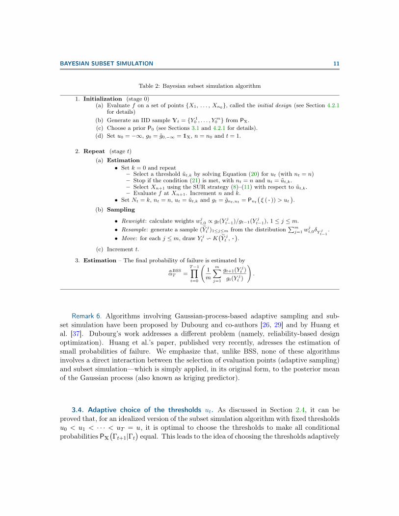
The BSS algorithm is presented in pseudo-code form in Table 2.
4See Section 4.2.1 for more information on the specific technique used in this article. Note that it isof course possible, albeit not required to use the BSS algorithm, to perform first a change of variables inorder to work, e.g., in the standard Gaussian space. Whether this will improve the performance of the BSSalgorithm is very difficult to say in general, and will depend on the example at hand.
5Other sampling strategies (also known as “sequential design”, or “active learning” methods) could beused as well. See [6] for a review and comparison of sampling criterions.
BAYESIAN SUBSET SIMULATION 11
Table 2: Bayesian subset simulation algorithm
1. Initialization (stage 0)(a) Evaluate f on a set of points {X1, . . . , Xn0}, called the initial design (see Section 4.2.1
for details)(b) Generate an IID sample Yt = {Y 1
0 , . . . , Ym0 } from PX.
(c) Choose a prior P0 (see Sections 3.1 and 4.2.1 for details).(d) Set u0 = −∞, g0 = g0,−∞ = 1X, n = n0 and t = 1.
2. Repeat (stage t)(a) Estimation
• Set k = 0 and repeat– Select a threshold ut,k by solving Equation (20) for ut (with nt = n)– Stop if the condition (21) is met, with nt = n and ut = ut,k.– Select Xn+1 using the SUR strategy (8)–(11) with respect to ut,k.– Evaluate f at Xn+1. Increment n and k.
• Set Nt = k, nt = n, ut = ut,k and gt = gnt,ut = Pnt(ξ ( · )) > ut
).
(b) Sampling
• Reweight : calculate weights wjt,0 ∝ gt(Yjt−1)/gt−1(Y jt−1), 1 ≤ j ≤ m.
• Resample: generate a sample (Y jt )1≤j≤m from the distribution∑mj=1 w
jt,0δY jt−1
.• Move: for each j ≤ m, draw Y jt v K
(Y jt , ·
).
(c) Increment t.
3. Estimation – The final probability of failure is estimated by
αBSST =
T−1∏t=0
(1
m
m∑j=1
gt+1(Y jt )
gt(Yjt )
).
Remark 6. Algorithms involving Gaussian-process-based adaptive sampling and sub-set simulation have been proposed by Dubourg and co-authors [26, 29] and by Huang etal. [37]. Dubourg’s work addresses a different problem (namely, reliability-based designoptimization). Huang et al.’s paper, published very recently, adresses the estimation ofsmall probabilities of failure. We emphasize that, unlike BSS, none of these algorithmsinvolves a direct interaction between the selection of evaluation points (adaptive sampling)and subset simulation—which is simply applied, in its original form, to the posterior meanof the Gaussian process (also known as kriging predictor).
3.4. Adaptive choice of the thresholds ut. As discussed in Section 2.4, it can beproved that, for an idealized version of the subset simulation algorithm with fixed thresholdsu0 < u1 < · · · < uT = u, it is optimal to choose the thresholds to make all conditionalprobabilities PX
(Γt+1|Γt
)equal. This leads to the idea of choosing the thresholds adaptively
12 JULIEN BECT, LING LI AND EMMANUEL VAZQUEZ
in such a way that, in the product estimate
αSST =
T∏t=1
1
m
m∑i=1
1Γt
(Y it−1
),
each term but the last is equal to some prescribed constant p0. In other words, ut is chosenas the (1− p0)-quantile of Yt−1. This idea was first suggested by ([2], Section 5.2), on theheuristic ground that the algorithm should perform well when the conditional probabilitiesare neither too small (otherwise they are hard to estimate) nor too large (otherwise a largenumber of stages is required).
Consider now an idealized BSS algorithm, where a) the initial design of experimentis independent of Y0, b) the SUR criterion is computed exactly, or using a discretizationscheme that does not use the Yt’s; c) the minimization of the SUR criterion is carriedout independently of the Yt’s and d) the particles Y j
t are independent and identically dis-tributed according to qt. Assumptions a)–c) ensure that the sequence of densities (qt)1≤t≤Tis deterministic given ξ. Then (see Appendix A),
(17) var
( αBSST
αBT
∣∣∣∣∣ ξ)
=1
m
T∑t=1
κt +O
(1
m2
),
where
(18) κt :=
∫Xg2t /gt−1 πX
(αBt )2 /αB
t−1
− 1.
Minimizing the leading term 1m
∑Tt=1 κt in (17) by an appropriate choice of thresholds is
not as straightforward as in the case of the subset simulation algorithm. Assuming thatgt−1 ≈ 1 wherever gt is not negligible (which is a reasonable assumption, since gt(x) =Pnt(ξ(x) > ut
)and ut > ut−1), we get∫
X
g2t /gt−1 πX ≈
∫X
g2t πX ≤
∫X
gt πX = αBt ,
and therefore the variance (17) is approximately upper-bounded by
(19)1
m
T∑t=1
(1− pBt ) /pB
t ,
where pBt := αB
t /αBt−1. Minimizing the approximate upper-bound (19) under the constraint
T∏t=1
pBt = αB
T
BAYESIAN SUBSET SIMULATION 13
leads to choosing the thresholds ut in such a way that pBt is the same for all stages t—that
is pBt = (αB
T )1/T . As a consequence, we propose to choose the thresholds adaptively usingthe condition that, at each stage (but the last), the natural estimator αBSS
t /αBSSt−1 of pB
t isequal to some prescribed probability p0. Owing to (15), this amounts to choosing ut insuch a way that
(20)1
m
m∑i=1
gt(Yit−1)
gt−1(Y it−1)
= p0.
should be satisfied.Equation (20) is easy to solve, since the left-hand side is a strictly decreasing and
continuous function of ut (to be precise, continuity holds under the assumption that theposterior variance of ξ does not vanish on one of the particles). In practice, we solve (20)each time a new evaluation is made, which yields a sequence of intermediate thresholds(denoted by ut,0, ut,1. . . in Table 2) at each stage t ≥ 1. The actual value of ut at stage tis only known after the last evaluation of stage t.
Remark 7. Alternatively, the effective sample size (ESS) could be used to select thethresholds, as proposed by [22]. This idea will not be pursued in this paper. The thresholdselected by the ESS-based approach will be close to the threshold selected by Equation (20)when the all the ratios gt(Y i
t−1)/gt−1(Y it−1), or most of them, are either close to zero or
close to one.
3.5. Adaptive choice of the number Nt of evaluation at each stage. In this section,we propose a technique to choose adaptively the number Nt of evaluations of f that mustbe done at each stage of the algorithm.
Assume that t ≥ 1 is the current stage number; at the beginning of the stage, nt−1 evalu-ations are available from previous stages. After several additional evaluations, the numberof available observations of f is n ≥ nt−1. We propose to stop adding new evaluationswhen the expected error of estimation of the set Γt, measured by En
(PX
(Γt 4 Γn,ut
)),
becomes smaller than some prescribed fraction ηt of its expected volume En (PX (Γt)) un-der PX. Writing these two quantities as
En (PX (Γt)) =
∫X
gn,ut(x)πX(x) dx = αBt−1
∫X
gn,ut(x)
gt−1(x)qt−1(x) dx,
En(PX
(Γ 4 Γn,ut
))=
∫X
τn,ut(x)πX(x) dx = αBt−1
∫X
τn,ut(x)
gt−1(x)qt−1(x) dx,
where gn,ut and τn,ut have been defined in Section 3.1, and estimating the integrals on theright-hand side using the SMC sample Yt−1, we end up with the stopping condition
1
m
m∑i=1
τn,ut(Y it−1
)gt−1
(Y it−1
) ≤ ηt ·1
m
m∑i=1
gn,ut(Y it−1
)gt−1
(Y it−1
) .
14 JULIEN BECT, LING LI AND EMMANUEL VAZQUEZ
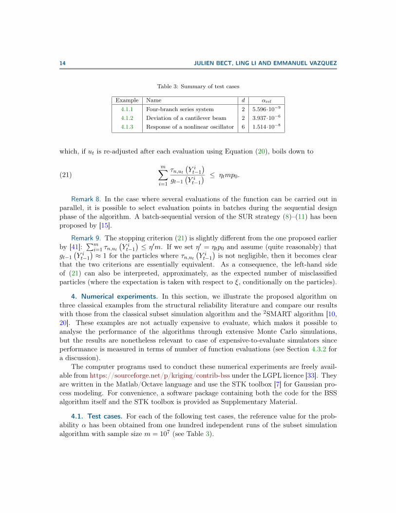
Table 3: Summary of test cases
Example Name d αref
4.1.1 Four-branch series system 2 5.596·10−9
4.1.2 Deviation of a cantilever beam 2 3.937·10−6
4.1.3 Response of a nonlinear oscillator 6 1.514·10−8
which, if ut is re-adjusted after each evaluation using Equation (20), boils down to
(21)m∑i=1
τn,ut(Y it−1
)gt−1
(Y it−1
) ≤ ηtmp0.
Remark 8. In the case where several evaluations of the function can be carried out inparallel, it is possible to select evaluation points in batches during the sequential designphase of the algorithm. A batch-sequential version of the SUR strategy (8)–(11) has beenproposed by [15].
Remark 9. The stopping criterion (21) is slightly different from the one proposed earlierby [41]:
∑mi=1 τn,ut
(Y it−1
)≤ η′m. If we set η′ = ηtp0 and assume (quite reasonably) that
gt−1
(Y it−1
)≈ 1 for the particles where τn,ut
(Y it−1
)is not negligible, then it becomes clear
that the two criterions are essentially equivalent. As a consequence, the left-hand sideof (21) can also be interpreted, approximately, as the expected number of misclassifiedparticles (where the expectation is taken with respect to ξ, conditionally on the particles).
4. Numerical experiments. In this section, we illustrate the proposed algorithm onthree classical examples from the structural reliability literature and compare our resultswith those from the classical subset simulation algorithm and the 2SMART algorithm [10,20]. These examples are not actually expensive to evaluate, which makes it possible toanalyse the performance of the algorithms through extensive Monte Carlo simulations,but the results are nonetheless relevant to case of expensive-to-evaluate simulators sinceperformance is measured in terms of number of function evaluations (see Section 4.3.2 fora discussion).
The computer programs used to conduct these numerical experiments are freely avail-able from https://sourceforge.net/p/kriging/contrib-bss under the LGPL licence [33]. Theyare written in the Matlab/Octave language and use the STK toolbox [7] for Gaussian pro-cess modeling. For convenience, a software package containing both the code for the BSSalgorithm itself and the STK toolbox is provided as Supplementary Material.
4.1. Test cases. For each of the following test cases, the reference value for the prob-ability α has been obtained from one hundred independent runs of the subset simulationalgorithm with sample size m = 107 (see Table 3).
BAYESIAN SUBSET SIMULATION 15
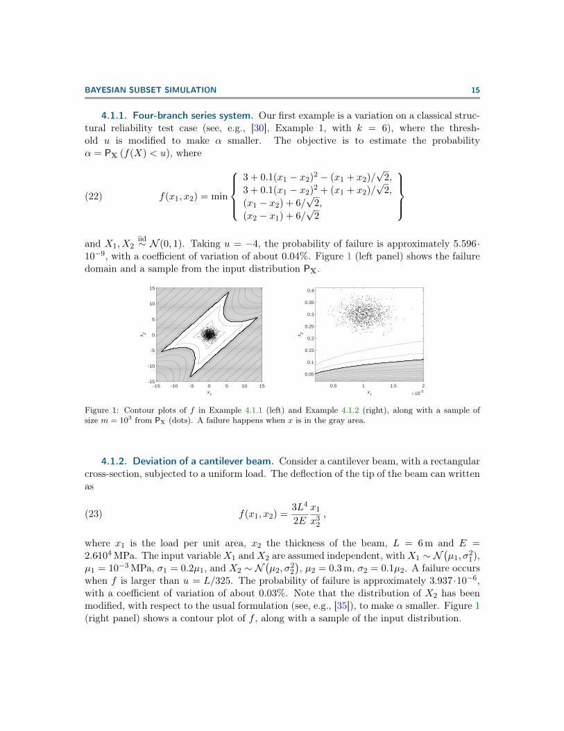
4.1.1. Four-branch series system. Our first example is a variation on a classical struc-tural reliability test case (see, e.g., [30], Example 1, with k = 6), where the thresh-old u is modified to make α smaller. The objective is to estimate the probabilityα = PX (f(X) < u), where
(22) f(x1, x2) = min
3 + 0.1(x1 − x2)2 − (x1 + x2)/
√2,
3 + 0.1(x1 − x2)2 + (x1 + x2)/√
2,
(x1 − x2) + 6/√
2,
(x2 − x1) + 6/√
2
and X1, X2
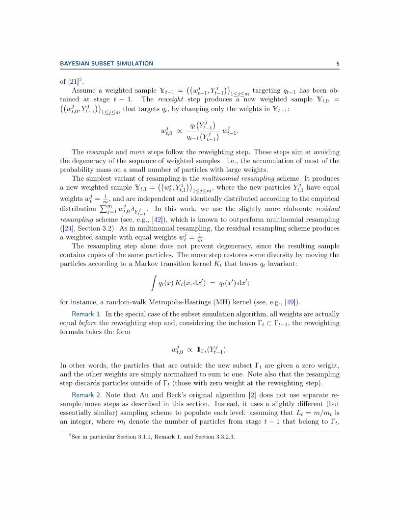
iid∼ N (0, 1). Taking u = −4, the probability of failure is approximately 5.596·10−9, with a coefficient of variation of about 0.04%. Figure 1 (left panel) shows the failuredomain and a sample from the input distribution PX.
x1
-15 -10 -5 0 5 10 15
x2
-15
-10
-5
0
5
10
15
x1 ×10-3
0.5 1 1.5 2
x2
0.05
0.1
0.15
0.2
0.25
0.3
0.35
0.4
Figure 1: Contour plots of f in Example 4.1.1 (left) and Example 4.1.2 (right), along with a sample ofsize m = 103 from PX (dots). A failure happens when x is in the gray area.
4.1.2. Deviation of a cantilever beam. Consider a cantilever beam, with a rectangularcross-section, subjected to a uniform load. The deflection of the tip of the beam can writtenas
(23) f(x1, x2) =3L4
2E
x1
x32
,
where x1 is the load per unit area, x2 the thickness of the beam, L = 6 m and E =2.6·104 MPa. The input variableX1 andX2 are assumed independent, withX1 ∼ N
(µ1, σ
21),
µ1 = 10−3 MPa, σ1 = 0.2µ1, and X2 ∼ N(µ2, σ
22
), µ2 = 0.3 m, σ2 = 0.1µ2. A failure occurs
when f is larger than u = L/325. The probability of failure is approximately 3.937·10−6,with a coefficient of variation of about 0.03%. Note that the distribution of X2 has beenmodified, with respect to the usual formulation (see, e.g., [35]), to make α smaller. Figure 1(right panel) shows a contour plot of f , along with a sample of the input distribution.
16 JULIEN BECT, LING LI AND EMMANUEL VAZQUEZ
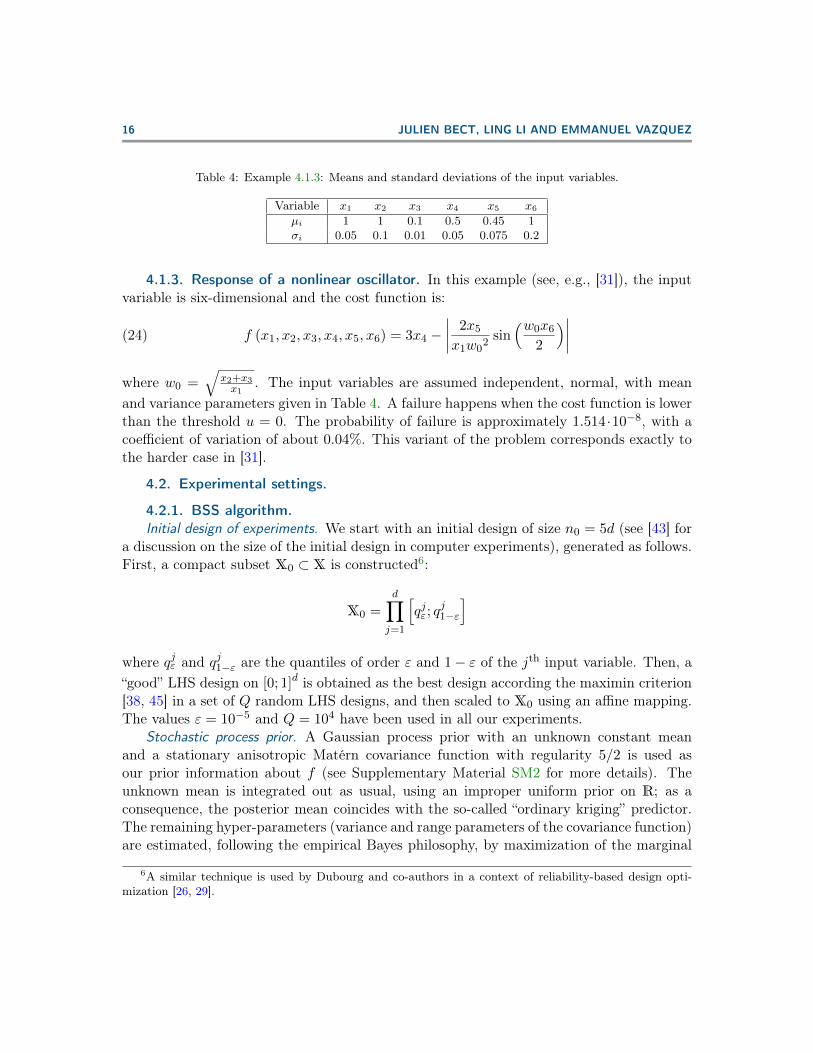
Table 4: Example 4.1.3: Means and standard deviations of the input variables.
Variable x1 x2 x3 x4 x5 x6
µi 1 1 0.1 0.5 0.45 1σi 0.05 0.1 0.01 0.05 0.075 0.2
4.1.3. Response of a nonlinear oscillator. In this example (see, e.g., [31]), the inputvariable is six-dimensional and the cost function is:
(24) f (x1, x2, x3, x4, x5, x6) = 3x4 −∣∣∣∣ 2x5
x1w02
sin(w0x6
2
)∣∣∣∣where w0 =
√x2+x3x1
. The input variables are assumed independent, normal, with meanand variance parameters given in Table 4. A failure happens when the cost function is lowerthan the threshold u = 0. The probability of failure is approximately 1.514 ·10−8, with acoefficient of variation of about 0.04%. This variant of the problem corresponds exactly tothe harder case in [31].
4.2. Experimental settings.
4.2.1. BSS algorithm.Initial design of experiments. We start with an initial design of size n0 = 5d (see [43] for
a discussion on the size of the initial design in computer experiments), generated as follows.First, a compact subset X0 ⊂ X is constructed6:
X0 =d∏j=1
[qjε; q
j1−ε
]where qjε and qj1−ε are the quantiles of order ε and 1− ε of the jth input variable. Then, a“good” LHS design on [0; 1]d is obtained as the best design according the maximin criterion[38, 45] in a set of Q random LHS designs, and then scaled to X0 using an affine mapping.The values ε = 10−5 and Q = 104 have been used in all our experiments.
Stochastic process prior. A Gaussian process prior with an unknown constant meanand a stationary anisotropic Matérn covariance function with regularity 5/2 is used asour prior information about f (see Supplementary Material SM2 for more details). Theunknown mean is integrated out as usual, using an improper uniform prior on R; as aconsequence, the posterior mean coincides with the so-called “ordinary kriging” predictor.The remaining hyper-parameters (variance and range parameters of the covariance function)are estimated, following the empirical Bayes philosophy, by maximization of the marginal
6A similar technique is used by Dubourg and co-authors in a context of reliability-based design opti-mization [26, 29].
BAYESIAN SUBSET SIMULATION 17
likelihood7. The hyper-parameters are estimated first on the data from the initial design,and then re-estimated after each new evaluation. In practice, we recommend to check theestimated parameters every once in a while using, e.g., leave-one-out cross-validation.
SMC parameters. Several values of the sample size m will be tested to study therelation between the variance of the estimator and the number of evaluations: m ∈{500, 1000, 2000, . . .}. Several iterations of an adaptive Gaussian Random Walk Metropolis-Hastings (RWMH) algorithm, fully described in Supplementary Material SM3, are used forthe move step of the algorithm.
Stopping criterion for the SUR strategy. The number of evaluations selected using theSUR strategy is determined adaptively, using the stopping criterion (21) from Section 3.5,with ηt = 0.5 for all t < T (i.e., for all intermediate stages) and ηT = 0.1 δm,T where δm,T isthe estimated coefficient of variation for the SMC estimator αBSS
T of αBT (see Appendix A).
Furthermore, we require for robustness a minimal number Nmin of evaluations at each stage,with Nmin = 2 in all our simulations.
Adaptive choice of the thresholds. The successive thresholds ut are chosen using theadaptive rule proposed in Section 3.4, Equation (20), with p0 = 0.1. This value has beenfound experimentally to be neither too large (to avoid having a large number of stages) nottoo small (to avoid losing too many particles during the resampling step)8.
4.2.2. Subset simulation algorithm. The parameters used for the subset simulationalgorithm are exactly the same, in all our simulations, as those used in the “SMC part” ofthe BSS algorithm (see Section 4.2.1). In particular, the numberm0 of surviving particles ateach stage is determined according to the rule p0 = m0
m = 0.1 (see Table 1), and the adaptiveMCMC algorithm described in Supplementary Material SM3 is used to move the particles.The number of evaluations made by the subset simulation algorithm is considered to bem + (T − 1) (1− p0)m, as explained in Section 2.4—in other words, in order to make thecomparison as fair as possible, the additional evaluations required by the adaptive MCMCprocedure are not taken into account.
4.2.3. 2SMART algorithm. 2SMART [10, 20] is another algorithm for the estimationof small probabilities, which is based on the combination of subset simulation with SupportVector Machines (SVM). We will present results obtained using the implementation of2SMART proposed in the software package FERUM 4.1 [8], with all parameters set to theirdefault values (which are equal to the values given in [10]).
Remark 10. Several other methods addressing the estimation of small probabilities offailure for expensive-to-evaluate functions have appeared recently in the structural relia-bility literature [4, 9, 12, 31, 37]. 2SMART was selected as a reference method due to the
7Used in combination with a uniform prior for the mean, for this specific model, the MML method isequivalent to the Restricted Maximum Likelihood (ReML) method advocated by [51], Section 6.4.
8Note that the considerations of Remark 4 on the choice of p0 are not relevant here, since the computa-tional cost of our method is mainly determined by the number of function evaluations, which is not directlyrelated to the number of particles to be simulated. See also Supplementary Material SM4.
18 JULIEN BECT, LING LI AND EMMANUEL VAZQUEZ
availability of a free software implementation in FERUM. A more comprehensive benchmarkis left for future work.
4.3. Results.
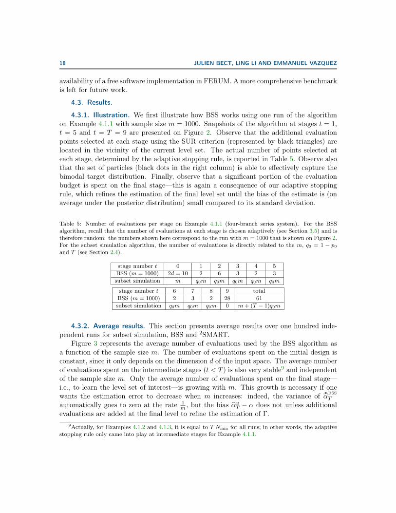
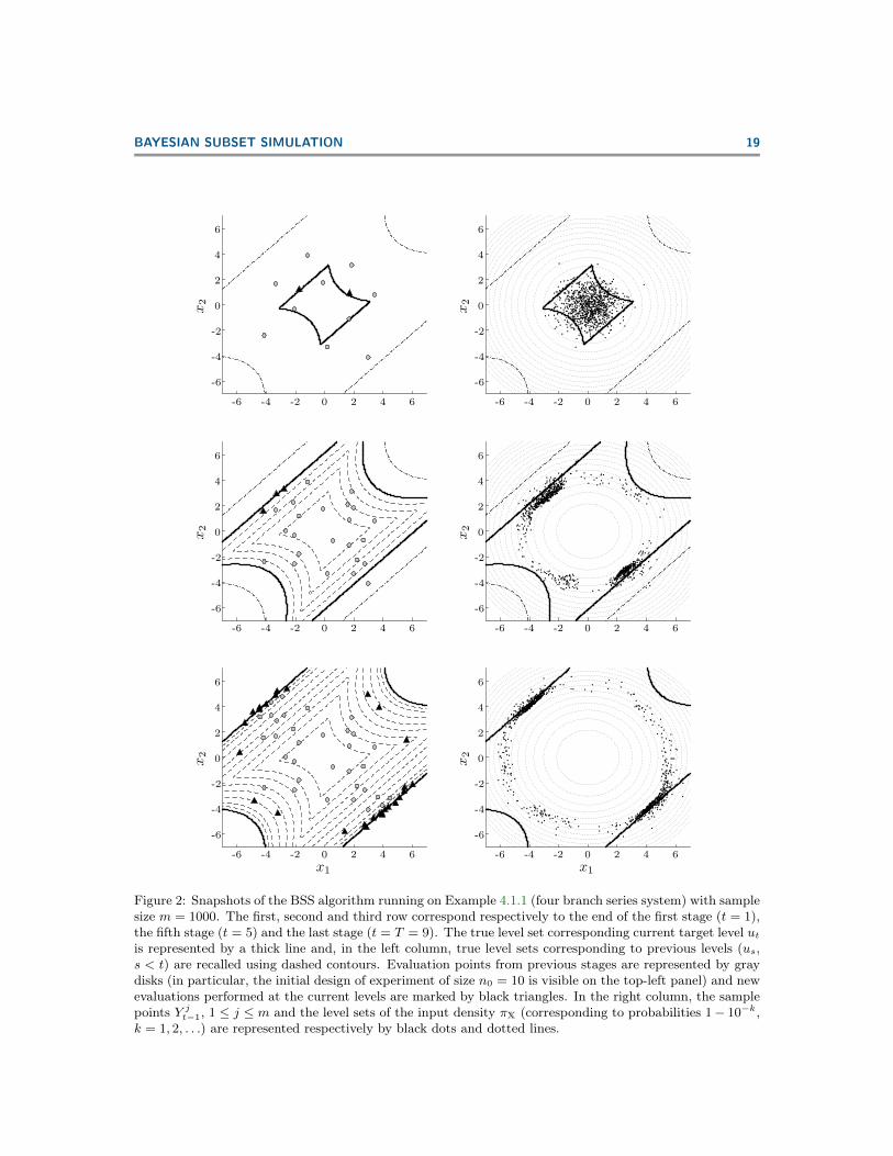
4.3.1. Illustration. We first illustrate how BSS works using one run of the algorithmon Example 4.1.1 with sample size m = 1000. Snapshots of the algorithm at stages t = 1,t = 5 and t = T = 9 are presented on Figure 2. Observe that the additional evaluationpoints selected at each stage using the SUR criterion (represented by black triangles) arelocated in the vicinity of the current level set. The actual number of points selected ateach stage, determined by the adaptive stopping rule, is reported in Table 5. Observe alsothat the set of particles (black dots in the right column) is able to effectively capture thebimodal target distribution. Finally, observe that a significant portion of the evaluationbudget is spent on the final stage—this is again a consequence of our adaptive stoppingrule, which refines the estimation of the final level set until the bias of the estimate is (onaverage under the posterior distribution) small compared to its standard deviation.
Table 5: Number of evaluations per stage on Example 4.1.1 (four-branch series system). For the BSSalgorithm, recall that the number of evaluations at each stage is chosen adaptively (see Section 3.5) and istherefore random: the numbers shown here correspond to the run with m = 1000 that is shown on Figure 2.For the subset simulation algorithm, the number of evaluations is directly related to the m, q0 = 1 − p0
and T (see Section 2.4).
stage number t 0 1 2 3 4 5
BSS (m = 1000) 2d = 10 2 6 3 2 3
subset simulation m q0m q0m q0m q0m q0m
stage number t 6 7 8 9 totalBSS (m = 1000) 2 3 2 28 61
subset simulation q0m q0m q0m 0 m+ (T − 1)q0m
4.3.2. Average results. This section presents average results over one hundred inde-pendent runs for subset simulation, BSS and 2SMART.
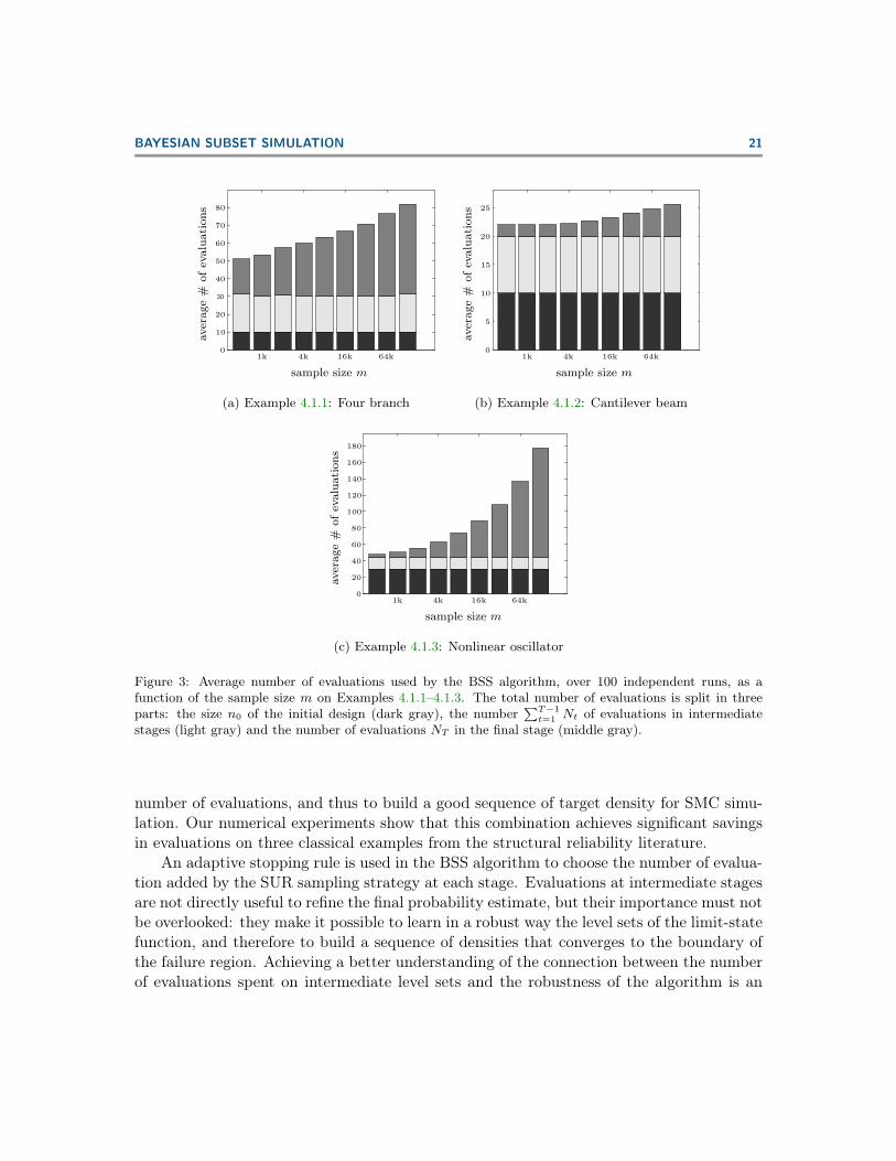
Figure 3 represents the average number of evaluations used by the BSS algorithm asa function of the sample size m. The number of evaluations spent on the initial design isconstant, since it only depends on the dimension d of the input space. The average numberof evaluations spent on the intermediate stages (t < T ) is also very stable9 and independentof the sample size m. Only the average number of evaluations spent on the final stage—i.e., to learn the level set of interest—is growing with m. This growth is necessary if onewants the estimation error to decrease when m increases: indeed, the variance of αBSS
T
automatically goes to zero at the rate 1m , but the bias αB
T − α does not unless additionalevaluations are added at the final level to refine the estimation of Γ.
9Actually, for Examples 4.1.2 and 4.1.3, it is equal to T Nmin for all runs; in other words, the adaptivestopping rule only came into play at intermediate stages for Example 4.1.1.
BAYESIAN SUBSET SIMULATION 19PSfrag
x2
-6
-6
-4
-4
-2
-2
0
0
2
2
4
4
6
6
x2
-6
-6
-4
-4
-2
-2
0
0
2
2
4
4
6
6
x2
-6
-6
-4
-4
-2
-2
0
0
2
2
4
4
6
6
x2
-6
-6
-4
-4
-2
-2
0
0
2
2
4
4
6
6
x2
-6
-6
-4
-4
-2
-2
0
0
2
2
4
4
6
6
x1
x2
-6
-6
-4
-4
-2
-2
0
0
2
2
4
4
6
6
x1
Figure 2: Snapshots of the BSS algorithm running on Example 4.1.1 (four branch series system) with samplesize m = 1000. The first, second and third row correspond respectively to the end of the first stage (t = 1),the fifth stage (t = 5) and the last stage (t = T = 9). The true level set corresponding current target level utis represented by a thick line and, in the left column, true level sets corresponding to previous levels (us,s < t) are recalled using dashed contours. Evaluation points from previous stages are represented by graydisks (in particular, the initial design of experiment of size n0 = 10 is visible on the top-left panel) and newevaluations performed at the current levels are marked by black triangles. In the right column, the samplepoints Y jt−1, 1 ≤ j ≤ m and the level sets of the input density πX (corresponding to probabilities 1− 10−k,k = 1, 2, . . .) are represented respectively by black dots and dotted lines.
20 JULIEN BECT, LING LI AND EMMANUEL VAZQUEZ
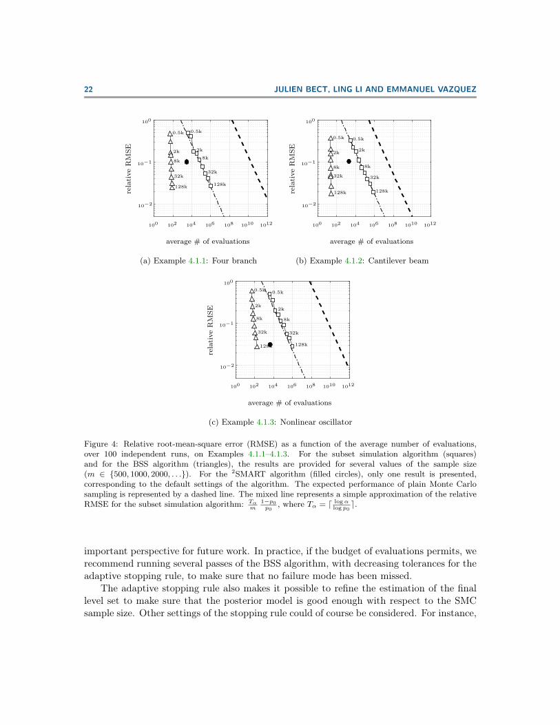
Figure 4 represents the relative Root-Mean-Square Error (RMSE) of all three algo-rithms, as a function of the average number of evaluations. For the subset simulationalgorithm, the number of evaluations is directly proportional to m and the RMSE de-creases as expected like 1
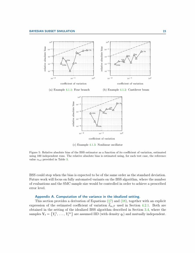
m (with a constant much smaller than that of plain Monte Carlosimulation). 2SMART clearly outperforms subset simulation, but offers no simple way oftuning the accuracy of the final estimate (which is why only one result is presented, usingthe default settings of the algorithm). Finally, BSS clearly and consistently outperformsboth 2SMART and subset simulation on these three examples: the relative RMSE goes tozero at a rate much faster than subset simulation’s (a feature that is made possible by thesmoothness of the limit-state function, which is leveraged by the Gaussian process model),and the sample size m is the only tuning parameters that needs to be acted upon in orderchange the accuracy of the final estimate. Figure 5 provides more insight into the error ofthe BSS estimate by confirming that, as intended by design of the adaptive stopping rule,variance is the main component of the RMSE (in other words, the bias is negligible in theseexamples).
Finally, note that the BSS estimation involves a computational overhead with respectto subset simulation. A careful analysis of the run times of BSS on the three examples(provided as Supplementary Material SM4.1) reveals that the computational overhead ofBSS is approximately equal to C0 + C1mNSUR, where NSUR the total number of eval-uations selected using the SUR criterion (i.e., all evaluations except the initial design ofexperiments). This shows that, in our implementation, the most time-consuming part ofthe algorithm is the selection of additional evaluation points using the SUR criterion. How-ever, in spite of its computational overhead, BSS is preferable to the subset simulationalgorithm in terms of computation time, on the three test cases, as soon as the evalua-tion time τsim of f is large enough—larger than, say, 10 ms for the considered range ofrelative RMSE (see Supplementary Material SM4.2 for details). Consider for instance Ex-ample 4.1.1 with τsim = 1 s: BSS with sample size m = 8000 achieves a relative RMSE ofapproximately 10% in about 3 minutes10 while subset simulation requires about 19 hoursto achieve a comparable accuracy.
5. Discussion. We propose an algorithm called Bayesian subset simulation for the es-timation of small probabilities of failure—or more generally the estimation of the volumeof excursion of a function above a threshold—when the limit-state function is expensive toevaluate. This new algorithm is built upon two key techniques: the SMC method known assubset simulation or adaptive multilevel splitting on the one hand, and the Bayesian (Gaus-sian process based) SUR sampling strategy on the other hand. SMC simulation providesthe means for evaluating the Bayesian estimate of the probability of failure, and to evaluateand optimize the SUR sampling criterion. In turn, the SUR sampling strategy makes itpossible to estimate the level sets of the (smooth) limit-state function using a restricted
10This computation time can be further decomposed as follows: 1 minute of evaluation time, correspond-ing to N = 63.2 evaluations on average (see Figure 3) and 2 minutes of algorithm overhead.
BAYESIAN SUBSET SIMULATION 21
30
sample size m
average#
ofevaluations
1k 4k 16k 64k0
10
20
40
50
60
70
80
(a) Example 4.1.1: Four branch
sample size m
average#
ofevaluations
1k 4k 16k 64k0
5
10
15
20
25
(b) Example 4.1.2: Cantilever beam
sample size m
average#
ofevaluations
1k 4k 16k 64k0
20
40
60
80
100
120
140
160
180
(c) Example 4.1.3: Nonlinear oscillator
Figure 3: Average number of evaluations used by the BSS algorithm, over 100 independent runs, as afunction of the sample size m on Examples 4.1.1–4.1.3. The total number of evaluations is split in threeparts: the size n0 of the initial design (dark gray), the number
∑T−1t=1 Nt of evaluations in intermediate
stages (light gray) and the number of evaluations NT in the final stage (middle gray).
number of evaluations, and thus to build a good sequence of target density for SMC simu-lation. Our numerical experiments show that this combination achieves significant savingsin evaluations on three classical examples from the structural reliability literature.
An adaptive stopping rule is used in the BSS algorithm to choose the number of evalua-tion added by the SUR sampling strategy at each stage. Evaluations at intermediate stagesare not directly useful to refine the final probability estimate, but their importance must notbe overlooked: they make it possible to learn in a robust way the level sets of the limit-statefunction, and therefore to build a sequence of densities that converges to the boundary ofthe failure region. Achieving a better understanding of the connection between the numberof evaluations spent on intermediate level sets and the robustness of the algorithm is an
22 JULIEN BECT, LING LI AND EMMANUEL VAZQUEZ
0.5k0.5k
2k2k
8k8k
32k
32k
128k128k
average # of evaluations
relativeRMSE
100
102
104
106
108
1010
1012
100
10−1
10−2
(a) Example 4.1.1: Four branch
0.5k0.5k
2k2k
8k8k
32k32k
128k128k
average # of evaluations
relativeRMSE
100
102
104
106
108
1010
1012
100
10−1
10−2
(b) Example 4.1.2: Cantilever beam
0.5k0.5k
2k2k
8k8k
32k32k
128k128k
average # of evaluations
relativeRMSE
100
102
104
106
108
1010
1012
100
10−1
10−2
(c) Example 4.1.3: Nonlinear oscillator
Figure 4: Relative root-mean-square error (RMSE) as a function of the average number of evaluations,over 100 independent runs, on Examples 4.1.1–4.1.3. For the subset simulation algorithm (squares)and for the BSS algorithm (triangles), the results are provided for several values of the sample size(m ∈ {500, 1000, 2000, . . .}). For the 2SMART algorithm (filled circles), only one result is presented,corresponding to the default settings of the algorithm. The expected performance of plain Monte Carlosampling is represented by a dashed line. The mixed line represents a simple approximation of the relativeRMSE for the subset simulation algorithm: Tα
m1−p0p0
, where Tα = d logαlog p0
e.
important perspective for future work. In practice, if the budget of evaluations permits, werecommend running several passes of the BSS algorithm, with decreasing tolerances for theadaptive stopping rule, to make sure that no failure mode has been missed.
The adaptive stopping rule also makes it possible to refine the estimation of the finallevel set to make sure that the posterior model is good enough with respect to the SMCsample size. Other settings of the stopping rule could of course be considered. For instance,
BAYESIAN SUBSET SIMULATION 23
0.5k
2k
8k
32k
128k
coefficient of variation
relativeabsolutebias
10−2
10−1
100
10−4
10−3
10−2
10−1
100
(a) Example 4.1.1: Four branch
0.5k
2k8k
32k
128k
coefficient of variation
relativeabsolutebias
10−2
10−1
100
10−4
10−3
10−2
10−1
100
(b) Example 4.1.2: Cantilever beam
0.5k
2k
8k
32k
128k
coefficient of variation
relativeabsolutebias
10−2
10−1
100
10−4
10−3
10−2
10−1
100
(c) Example 4.1.3: Nonlinear oscillator
Figure 5: Relative absolute bias of the BSS estimator as a function of its coefficient of variation, estimatedusing 100 independent runs. The relative absolute bias is estimated using, for each test case, the referencevalue αref provided in Table 3.
BSS could stop when the bias is expected to be of the same order as the standard deviation.Future work will focus on fully automated variants on the BSS algorithm, where the numberof evaluations and the SMC sample size would be controlled in order to achieve a prescribederror level.
Appendix A. Computation of the variance in the idealized setting.This section provides a derivation of Equations (17) and (18), together with an explicit
expression of the estimated coefficient of variation δm,T used in Section 4.2.1. Both areobtained in the setting of the idealized BSS algorithm described in Section 3.4, where thesamples Yt =
{Y 1t , . . . , Y
mt
}are assumed IID (with density qt) and mutually independent.

24 JULIEN BECT, LING LI AND EMMANUEL VAZQUEZ
Recall from Equation (16) that the BSS estimator can be written as
(25) αBSST =
T∏t=1
αBSStαBSSt−1
=T∏t=1
1
m
m∑j=1
gt(Yjt−1)
gt−1(Y jt−1)
=T∏t=1
pBSSt ,
where we have set, for all t ∈ {1, . . . , T},
pBSSt =
1
m
m∑j=1
gt(Yjt−1)
gt−1(Y jt−1)
.
Observe that the random variables pBSSt are independent, with mean
E(pBSS
t
)=
∫X
gtgt−1
qt−1 =
∫X
gtgt−1
gt−1 πXαBt−1
=αBt
αBt−1
= pBt
and variance
var(pBSS
t
)=
1
mvar
(gt(Y 1t−1
)gt−1
(Y 1t−1
))
=1
m
[∫X
g2t
g2t−1
gt−1 πXαBt−1
−(αBt
αBt−1
)2]
=1
m
[1
αBt−1
∫X
g2t
gt−1πX −
(αBt
αBt−1
)2]
=1
m(pBt )2 κt,
where κt is defined by (18). Therefore, the coefficients of variation δm,t of the sequenceof estimators αBSS
t obey the recurrence relation δ2m,t = 1
mκt +(1 + 1
mκt)δ2m,t−1, and we
conclude that
δ2m,T =
1
mκT +
(1 +
1
mκT
)1
mκT−1
+
(1 +
1
mκT
) (1 +
1
mκT−1
)1
mκT−2 + · · ·
=1
m
T∑t=1
κt +O
(1
m2
),
which proves Equations (17)–(18). We construct an estimator of the coefficient of variationrecursively, using the relation
δ2m,t =
1
mκt +
(1 +
1
mκt
)δ2m,t−1,
BAYESIAN SUBSET SIMULATION 25
with
κt =(pBSS
t
)−2· 1
m
m∑j=1
gt
(Y jt−1
)gt−1
(Y jt−1
) − pBSSt
2
.
References.[1] A. Arnaud, J. Bect, M. Couplet, A. Pasanisi, and E. Vazquez, Évaluation
d’un risque d’inondation fluviale par planification séquentielle d’expériences, in 42èmesJournées de Statistique (JdS 2010), Marseille, France, May 24–28, 2010.
[2] S. K. Au and J. Beck, Estimation of small failure probabilities in high dimensions bysubset simulation, Probab. Eng. Mech., 16 (2001), pp. 263–277.
[3] Y. Auffray, P. Barbillon, and J.-M. Marin, Bounding rare event probabilities incomputer experiments, Comput. Statist. Data Anal., 80 (2014), pp. 153–166.
[4] M. Balesdent, J. Morio, and J. Marzat, Kriging-based adaptive Importance Sam-pling algorithms for rare event estimation, Struct. Saf., 44 (2013), pp. 1–10.
[5] M. J. Bayarri, J. O. Berger, E. S. Calder, K. Dalbey, S. Lunagomez, A. K.Patra, E. B. Pitman, E. T. Spiller, and R. L. Wolpert, Using statistical andcomputer models to quantify volcanic hazards, Technometrics, 51 (2009), pp. 402–413.
[6] J. Bect, D. Ginsbourger, L. Li, V. Picheny, and E. Vazquez, Sequential designof computer experiments for the estimation of a probability of failure, Stat. Comput., 22(2012), pp. 773–793.
[7] J. Bect, E. Vazquez, et al., STK: a Small (Matlab/Octave) Toolbox for Kriging.Release 2.4 (to appear), 2016, http://kriging.sourceforge.net.
[8] J.-M. Bourinet, Ferum 4.1 user’s guide. http://www.ifma.fr/FERUM, 2010.[9] J.-M. Bourinet, Rare-event probability estimation with adaptive support vector regres-
sion surrogates, Reliab. Eng. Syst. Saf., 150 (2016), pp. 210–221.[10] J.-M. Bourinet, F. Deheeger, and M. Lemaire, Assessing small failure prob-
abilities by combined subset simulation and support vector machines, Struct. Saf., 33(2011), pp. 343–353.
[11] C.-E. Bréhier, L. Goudenège, and L. Tudela, Central limit theorem for adaptivemultilevel splitting estimators in an idealized setting, in Monte Carlo and Quasi-MonteCarlo Methods (MCQMC 2014), R. Cools and D. Nuyens, eds., Springer, 2016.
[12] F. Cadini, F. Santos, and E. Zio, An improved adaptive kriging-based importancetechnique for sampling multiple failure regions of low probability, Reliab. Eng. Syst. Saf.,131 (2014), pp. 109–117.
[13] C. Cannamela, J. Garnier, and B. Iooss, Controlled stratification for quantileestimation, Annals of Applied Statistics, 2 (2008), pp. 1554–1580.
[14] C. Chevalier, J. Bect, D. Ginsbourger, and I. Molchanov, Estimating andquantifying uncertainties on level sets using the Vorob’ev expectation and deviation withgaussian process models, in mODa 10 — Advances in Model-Oriented Design and Anal-
26 JULIEN BECT, LING LI AND EMMANUEL VAZQUEZ
ysis, Contributions to Statistics, Springer, 2013, pp. 35–43.[15] C. Chevalier, J. Bect, D. Ginsbourger, E. Vazquez, V. Picheny, and
Y. Richet, Fast parallel kriging-based stepwise uncertainty reduction with applicationto the identification of an excursion set, Technometrics, 56 (2013), pp. 455–465.
[16] N. Chopin, A sequential particle filter method for static models, Biometrika, 89 (2002),pp. 539–552.
[17] F. Cérou, P. Del Moral, T. Furon, and A. Guyader, Sequential Monte Carlofor rare event estimation, Stat. Comput., 22 (2012), pp. 795–808.
[18] E. De Rocquigny, N. Devictor, S. Tarantola, et al., Determination of therisk due to personal electronic devices (PEDs) carried out on radio-navigation systemsaboard aircraft, in [19], 2008, ch. 5, pp. 65–80.
[19] E. De Rocquigny, N. Devictor, S. Tarantola, et al., Uncertainty in industrialpractice, Wiley, 2008.
[20] F. Deheeger, Couplage mécano-fiabiliste: 2SMART – Méthodologie d’apprentissagestochastique en fiabilité, PhD thesis, Université B. Pascal (Clermont-Ferrand II), 2008.
[21] P. Del Moral, A. Doucet, and A. Jasra, Sequential Monte Carlo samplers, J. theRoyal Statistical Society: Series B (Statistical Methodology), 68 (2006), pp. 411–436.
[22] P. Del Moral, A. Doucet, and A. Jasra, An adaptive sequential Monte Carlomethod for approximate Bayesian computation, Stat. Comput., 22 (2012), pp. 1009–1020.
[23] P. Diaconis and S. Holmes, Three examples of Monte-Carlo Markov chains: atthe interface between statistical computing, computer science, and statistical mechanics,vol. 72 of IMA volumes in Mathematics and its Applications, Springer, 1995, pp. 43–56.
[24] R. Douc and O. Cappé, Comparison of resampling schemes for particle filtering, inProceedings of the 4th International Symposium on Image and Signal Processing andAnalysis (ISPA), 2005, pp. 64–69.
[25] R. Douc and E. Moulines, Limit theorems for weighted samples with applicationsto sequential Monte Carlo methods, The Annals of Statistics, 36 (2008), pp. 2344–2376.
[26] V. Dubourg, Adaptive surrogate models for reliability analysis and reliability-baseddesign optimization, PhD thesis, Université Blaise Pascal – Clermont II, 2011.
[27] V. Dubourg, F. Deheeger, and B. Sudret, Metamodel-based importance sam-pling for the simulation of rare events, in 11th International Conference on Applicationsof Statistics and Probability in Civil Engineering (ICASP 11), 2011.
[28] V. Dubourg, F. Deheeger, and B. Sudret, Metamodel-based importance sam-pling for structural reliability analysis, Probab. Eng. Mech., 33 (2013), pp. 47–57.
[29] V. Dubourg, B. Sudret, and J.-M. Bourinet, Reliability-based design optimiza-tion using kriging surrogates and subset simulation, Struct. Multiscip. Optim., 44 (2011),pp. 673–690.
[30] B. Echard, N. Gayton, and M. Lemaire, AK-MCS: An active learning reliabilitymethod combining kriging and Monte Carlo simulation, Struct. Saf., 33 (2011), pp. 145–154.
BAYESIAN SUBSET SIMULATION 27
[31] B. Echard, N. Gayton, M. Lemaire, and N. Relun, A combined importance sam-pling and kriging reliability method for small failure probabilities with time-demandingnumerical models, Reliab. Eng. Syst. Saf., 111 (2013), pp. 232–240.
[32] P. Feliot, J. Bect, and V. E., A Bayesian approach to constrained single- andmulti-objective optimization, J. Global Optim., (in press), pp. 1–37.
[33] Free Software Foundation, GNU Lesser General Public License, version 2.1,http://www.gnu.org/licenses/old-licenses/lgpl-2.1.html.
[34] E. Garcia, Electromagnetic compatibility uncertainty, risk, and margin management,IEEE Trans. Electromag. Compat., 52 (2010), pp. 3–10.
[35] N. Gayton, J. M. Bourinet, and M. Lemaire, CQ2RS: a new statistical approachto the response surface method for reliability analysis, Struct. Saf., 25 (2003), pp. 99–121.
[36] P. Glasserman, P. Heidelberger, P. Shahabuddin, and T. Zajic, Multilevelsplitting for estimating rare event probabilities, Oper. Res., 47 (1999), pp. 585–600.
[37] X. Huang, J. Chen, and H. Zhu, Assessing small failure probabilities by AK-SS: Anactive learning method combining kriging and subset simulation, Struct. Saf., 59 (2016),pp. 86–95.
[38] M. E. Johnson, L. M. Moore, and D. Ylvisaker, Minimax and maximin distancedesigns, J. Statist. Plan. Inference, 26 (1990), pp. 131–148.
[39] S. N. Jonkman, M. Kok, and J. K. Vrijling, Flood risk assessment in the nether-lands: A case study for dike ring south holland, Risk Analysis, 28 (2008), pp. 1357–1374.
[40] L. Li, Sequential Design of Experiments to Estimate a Probability of Failure, PhDthesis, Supélec, May 2012, https://tel.archives-ouvertes.fr/tel-00765457.
[41] L. Li, J. Bect, and E. Vazquez, Bayesian subset simulation: a kriging-based subsetsimulation algorithm for the estimation of small probabilities of failure, in Proceedingsof PSAM 11 & ESREL 2012, 25-29 June 2012, Helsinki, Finland., 2012.
[42] J. S. Liu, Monte Carlo strategies in scientific computing, Springer, 2008.[43] J. L. Loeppky, J. Sacks, and W. J. Welch, Choosing the sample size of a computer
experiment: A practical guide, Technometrics, 51 (2009), pp. 366–376.[44] R. E. Melchers, Structural Reliability: Analysis and Prediction. Second Edition.,
Wiley, 1999.[45] M. D. Morris and T. J. Mitchell, Exploratory designs for computational experi-
ments, J. Statist. Plan. Inference, 43 (1995), pp. 381–402.[46] J. Oakley, Estimating percentiles of uncertain computer code outputs, J. Roy. Statist.
Soc. Ser. C, 53 (2004), pp. 83–93.[47] P. P. O’Connor and A. Kleyner, Practical Reliability Engineering, Wiley, 2012.[48] M. Rausand and A. Hoyland, System reliability theory: models and statistical
methods (second edition), Wiley, 2004.[49] C. P. Robert and G. Casella, Monte Carlo statistical methods, 2nd edition,
Springer Verlag, 2004.[50] T. J. Santner, B. J. Williams, and W. Notz, The Design and Analysis of Com-
puter Experiments, Springer Verlag, 2003.
28 JULIEN BECT, LING LI AND EMMANUEL VAZQUEZ
[51] M. L. Stein, Interpolation of Spatial Data: Some Theory for Kriging, Springer, NewYork, 1999.
[52] E. Vazquez and J. Bect, A sequential Bayesian algorithm to estimate a probabilityof failure, in Proceedings of the 15th IFAC Symposium on System Identification, SYSID2009, Saint-Malo France, 2009.
[53] J. Villemonteix, E. Vazquez, and E. Walter, An informational approach tothe global optimization of expensive-to-evaluate functions, J. Global Optim., 44 (2009),pp. 509–534.
[54] P. H. Waarts, Structural reliability using finite element methods, PhD thesis, DelftUniversity of Technology, 2000.
[55] E. Zio and N. Pedroni, Estimation of the functional failure probability of a thermal-hydraulic passive system by subset simulation, Nuclear Eng. Design, 239 (2009), pp. 580–599.
[56] K. M. Zuev, J. L. Beck, S.-K. Au, and L. S. Katafygiotis, Bayesian post-processor and other enhancements of subset simulation for estimating failure probabilitiesin high dimensions, Computers & Structures, 92–93 (2012), pp. 283–296.
BAYESIAN SUBSET SIMULATION (SUPPLEMENTARY MATERIALS) 1
SUPPLEMENTARY MATERIALS
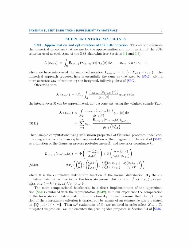
SM1. Approximation and optimization of the SUR criterion. This section discussesthe numerical procedure that we use for the approximation and optimization of the SURcriterion used at each stage of the BSS algorithm (see Sections 3.1 and 3.3):
Jn (xn+1) =
∫X
En,xn+1 (τn+1,ut(x)) πX(x) dx, nt−1 ≤ n ≤ nt − 1,
where we have introduced the simplified notation En,xn+1:= En
(·∣∣ Xn+1 = xn+1
). The
numerical approach proposed here is essentially the same as that used by [SM6], with amore accurate way of computing the integrand, following ideas of [SM2].
Observing that
Jn (xn+1) = αBt−1
∫X
En,xn+1 (τn+1,ut(x) )
gt−1(x)qt−1(x) dx,
the integral overX can be approximated, up to a constant, using the weighted sample Yt−1:
Jn (xn+1) ∝∫X
En,xn+1 (τn+1,ut(x))
gt−1(x)qt−1(x) dx
≈m∑j=1
wjt−1
En,xn+1 (τn+1,ut(x))|x=Y jt−1
gt−1
(Y jt−1
) .(SM1)
Then, simple computations using well-known properties of Gaussian processes under con-ditioning allow to obtain an explicit representation of the integrand, in the spirit of [SM2],as a function of the Gaussian process posterior mean ξn and posterior covariance kn:
En,xn+1 (τn+1,ut(x)) = Φ
(u− ξn(x)
σn(x)
)+ Φ
(u− ξn(x)
sn(x, xn+1)
)
− 2 Φ2
((uu
);
(ξn(x)
ξn(x)
),
(s2n(x, xn+1) s2
n(x, xn+1)s2n(x, xn+1) σn(x)2
)),(SM2)
where Φ is the cumulative distribution function of the normal distribution, Φ2 the cu-mulative distribution function of the bivariate normal distribution, σ2
n(x) = kn(x, x) ands2n(x, xn+1) = kn(x, xn+1)2/σn(xn+1)2.
The main computational bottleneck, in a direct implementation of the approxima-tion (SM1) combined with the representation (SM2), is in our experience the computationof the bivariate cumulative distribution function Φ2. Indeed, assume that the optimiza-tion of the approximate criterion is carried out by means of an exhaustive discrete searchon {Y j
t−1, 1 ≤ j ≤ m}. Then m2 evaluations of Φ2 are required in order select Xn+1. Tomitigate this problem, we implemented the pruning idea proposed in Section 3.4 of [SM6]:
2 JULIEN BECT, LING LI AND EMMANUEL VAZQUEZ
only a subset of size m0 ≤ m of the set of particles is actually used, both for the approx-imation the integral and for the optimization of the criterion. In this article, the size m0
is determined automatically as follows: first, for each particle Y jt−1, the current weighted
probability of misclassification
τ jn := wjt−1τn,ut
(Y jt−1
)/gt−1
(Y jt−1
)is computed. Then, the particules are sorted according to the value of τ jn, in decreasingorder: τϕ(1)
n ≥ τϕ(2)n ≥ . . . ≥ τ
ϕ(m)n , and m0 is set to min (mmax
0 ,m0(τn)), where m0(τn)is the smallest integer such that
m0∑j=1
τϕ(j)n ≥ ρ
m∑j=1
τ jn.
The values mmax0 = 1000 and ρ = 0.99 have been used in all our simulations.
SM2. Stochastic process prior. The stochastic process prior used for the numericalexperiments in this article is a rather standard Gaussian process model. We describe ithere in full detail for the sake of completeness. First, ξ is written as
ξ(x) = µ+ ξ0(x),
where µ ∈ R is an unknown constant mean and ξ0 a zero-mean stationary Gaussian processwith anisotropic covariance function
(SM3) k(x, y) = σ2κν
√√√√ d∑
i=1
(x[i] − y[i])2
ρ2i
, x, y ∈ Rd,
where x[i], y[i] denote the ith coordinate of x and y, and κν the Matérn correlation functionof regularity ν (see [SM8], Section 2.10). The scale parameters ρ1, . . . , ρd (characteristiccorrelation lengths) are usually called the range parameters of the covariance function.
In this article, the regularity parameter ν is set to the fixed value ν = 5/2, leading tothe following analytical expression for the Matérn correlation function:
(SM4) κν (h) =
(1 + h+
1
3h2
)exp
(−h), with h =
√10 |h| .
As a consequence, ξ is twice differentiable in the mean-square sense, with sample pathsalmost surely in the Sobolev space W s,2 for all s < 5/2 ([SM7], Theorem 3).
Remark SM1. The parameterization used in Equation (SM4) is the one advocatedin [SM8]. Other parameterizations are sometimes used in the literature; e.g., [SM5] useh =√
5 |h|.
BAYESIAN SUBSET SIMULATION (SUPPLEMENTARY MATERIALS) 3
SM3. Adaptive Metropolis-Hastings algorithm for the move step. A fixed number Sof iterations of a Gaussian Random Walk Metropolis-Hastings (RWMH) kernel is usedfor the move step, with adaptation of the standard deviations of the increments. Moreprecisely, for s = 1, 2, . . . , S, starting with the set of particles
(Y
(j)t,1
)1≤j≤m
produced by
the resampling step, we first produce perturbed particles:
Y(j)t,s = Y
(j)t,s + ΣRW,t,s Ut,s, 1 ≤ j ≤ m,
where ΣRW,t,s is a diagonal matrix and Ut,s a d-dimensional standard normal vector. Theperturbed particle is accepted as Y (j)
t,s+1 with probability
a(j)t,s = 1 ∧
qt
(Y
(j)t,s
)qt
(Y
(j)t,s
) ,and Y (j)
t,s is kept otherwise. The kth diagonal element σ(k)RW,t,s of ΣRW,t,s is initialized with
(SM5) σ(k)RW,1,1 = Cσ,init σ
(k)X ,
where σ(k)X is the standard deviation of the kth marginal of PX, and then updated using
(SM6) log σ(k)RW,t,s =
{log σ
(k)RW,t,s−1 + ∆σ/s if at,s > atarget
log σ(k)RW,t,s−1 −∆σ/s otherwise,
where σ(k)RW,t,−1 = σ
(k)RW,t−1,S , at,s = 1
m
∑mj=1 a
(j)t,s is the average acceptance probability and
atarget some prescribed target value.The following parameter values have been used for the numerical simulations presented
in this article: S = 10, Cσ,init = 2/√d, ∆σ = log(2) and atarget = 30%.
Remark SM2. The 1/√d scaling for the constant Cσ,init in (SM5) is motivated by the
well-known theorem of [SM6], which provides the optimal covariance matrix 2.382Σ/d fora Gaussian target with covariance matrix Σ in high dimension.
Remark SM3. The value ∆σ = log(2) that was used in the simulation turns out to betoo small to be a good general recommendation for a default value. Indeed, with S = 10steps of adaptation, it leads to a maximal adaptation factor of 21+ 1
2+...+ 1
10 ≈ 7.6, whichmight prove too small for some cases. The value ∆σ = log(10) is thus used as a defaultvalue in the Matlab/Octave program that is provided as Supplementary Material.
Remark SM4. The reader is referred to [SM9] and references therein for more informa-tion on adaptive MCMC algorithms, including adaptive scaling algorithms such as (SM6).Note, however, that the adaptation scheme proposed here is not strictly-speaking an adap-tive MCMC scheme, since we use the entire population of particles to estimate the accep-tance probability.

4 JULIEN BECT, LING LI AND EMMANUEL VAZQUEZ
Remark SM5. Our adaptive scheme (SM5)–(SM6) is admittedly very simple, but workswell in the examples of the paper. More refined adaptation schemes might be needed todeal with harder problems. For instance, it might become necessary to implement a trulyanisotropic adaptation of the covariance matrix, or to use different kernels in differentregions of the input space. Ideas from the adaptive SMC literature (see, e.g., [SM1, SM3,SM4]) could be leveraged to achieve these goals, which fall out of the scope of the presentpaper.
BAYESIAN SUBSET SIMULATION (SUPPLEMENTARY MATERIALS) 5
SM4. Run time of the BSS algorithm.
SM4.1. Overhead of the BSS algorithm. The median run times of the Bayesian subsetsimulation (BSS) and subset simulation (SS) algorithms on the three test cases of Section 4are reported in Table SM1. Since the function f in each of these examples is actually veryfast to evaluate, these run times provide a good indication of the numerical complexity ofthe algorithms. Consequently, they provide a measure of the overhead of the algorithm if itwere actually run on an expensive-to-evaluate function (i.e., the fraction of the computationtime not dedicated to evaluating the function).
As expected, because of the computations related to Gaussian process modeling, theoverhead of BSS is larger than the one of subset simulation, for a given sample size m. Inour implementation, this overhead, which we denote by τBSS,0, can be explained by a simplelinear model:
(SM7) τBSS,0 ≈ C0 + C1mNSUR
where m is the sample size and NSUR the total number of evaluations selected usingthe SUR criterion (i.e., all evaluations except the initial design of experiments). On ourstandard Intel-Nehalem-based workstation, an ordinary least-square regression using Equa-tion (SM7), on the 100 × 3 × 8 = 2400 points of our data set (100 runs on 3 cases with8 sample sizes), yields C0 ≈ 27.0 and C1 ≈ 5.2 10−5, with a coefficient of determinationof 97.2%. We conclude that the most time-consuming part of the algorithm is the selectionof additional evaluation points using the SUR criterion.
Remark SM6. Note that the computation time of BSS would grow as a functionof m2NSUR, instead of mNSUR, without the pruning idea explained in Section A.
SM4.2. Extrapolation to expensive-to-evaluate functions. Let us now extrapolatefrom the available data, obtained for cheap-to-evaluate test functions, to the case of a non-negligible evaluation time. To this end, assume that each evaluation actually costs τsim incomputation time. Then, the total run time of BSS becomes
(SM8) τBSS = τBSS,0 + τsimN,
where N is the total number of evaluations. For a given test case and a given samplesize m, denote by N the average total number of evaluation, τBSS,0 the average overheadand rRMSE the relative root-mean-square error (computed using 100 runs of BSS). Theefficiency of BSS with respect to the subset simulation algorithm can be measured by theratio
(SM9) εBSS | SS =τSS
τBSS
where τBSS = τBSS,0 + τsim N is the average total run time for BSS, and τSS is an approx-imation of the time it would take for subset simulation to reach the same relative RMSE,
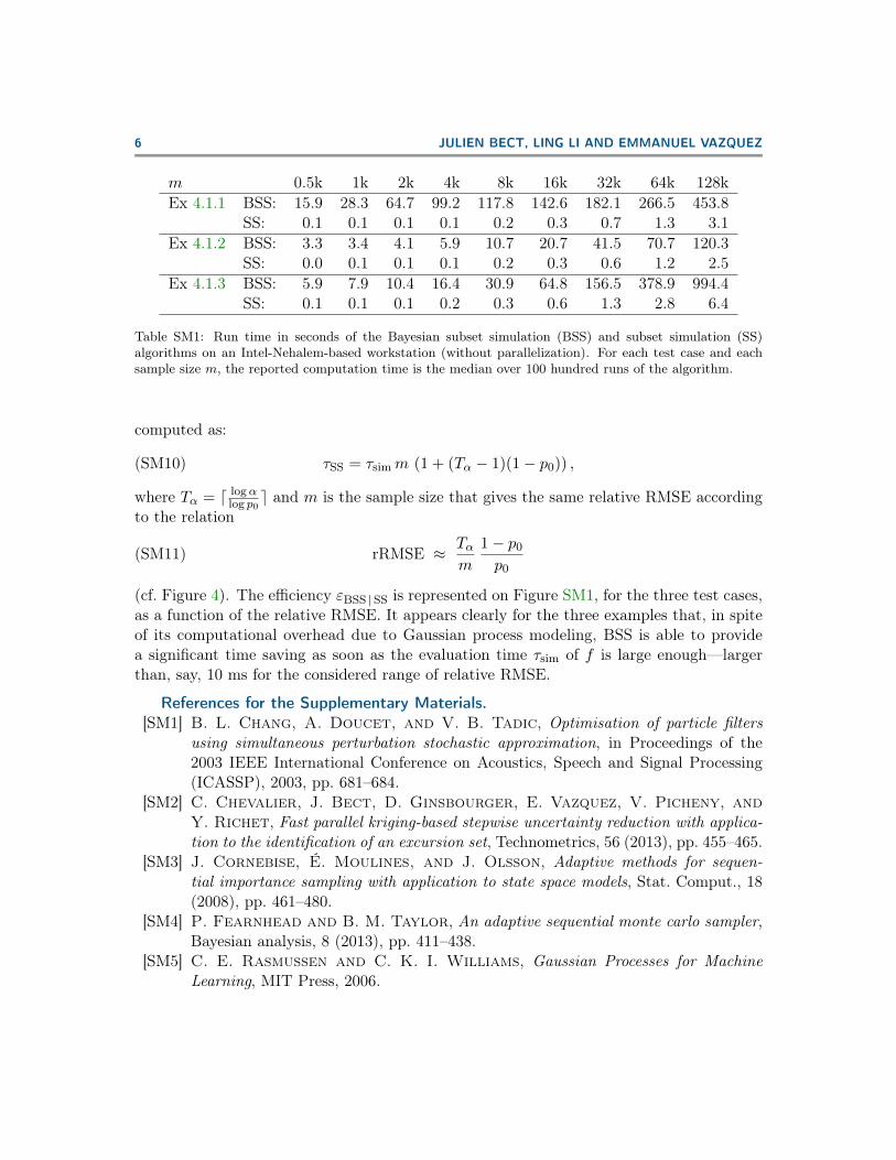
6 JULIEN BECT, LING LI AND EMMANUEL VAZQUEZ
m 0.5k 1k 2k 4k 8k 16k 32k 64k 128kEx 4.1.1 BSS: 15.9 28.3 64.7 99.2 117.8 142.6 182.1 266.5 453.8
SS: 0.1 0.1 0.1 0.1 0.2 0.3 0.7 1.3 3.1Ex 4.1.2 BSS: 3.3 3.4 4.1 5.9 10.7 20.7 41.5 70.7 120.3
SS: 0.0 0.1 0.1 0.1 0.2 0.3 0.6 1.2 2.5Ex 4.1.3 BSS: 5.9 7.9 10.4 16.4 30.9 64.8 156.5 378.9 994.4
SS: 0.1 0.1 0.1 0.2 0.3 0.6 1.3 2.8 6.4
Table SM1: Run time in seconds of the Bayesian subset simulation (BSS) and subset simulation (SS)algorithms on an Intel-Nehalem-based workstation (without parallelization). For each test case and eachsample size m, the reported computation time is the median over 100 hundred runs of the algorithm.
computed as:
(SM10) τSS = τsimm (1 + (Tα − 1)(1− p0)) ,
where Tα = d logαlog p0
e and m is the sample size that gives the same relative RMSE accordingto the relation
(SM11) rRMSE ≈ Tαm
1− p0
p0
(cf. Figure 4). The efficiency εBSS | SS is represented on Figure SM1, for the three test cases,as a function of the relative RMSE. It appears clearly for the three examples that, in spiteof its computational overhead due to Gaussian process modeling, BSS is able to providea significant time saving as soon as the evaluation time τsim of f is large enough—largerthan, say, 10 ms for the considered range of relative RMSE.
References for the Supplementary Materials.[SM1] B. L. Chang, A. Doucet, and V. B. Tadic, Optimisation of particle filters
using simultaneous perturbation stochastic approximation, in Proceedings of the2003 IEEE International Conference on Acoustics, Speech and Signal Processing(ICASSP), 2003, pp. 681–684.
[SM2] C. Chevalier, J. Bect, D. Ginsbourger, E. Vazquez, V. Picheny, andY. Richet, Fast parallel kriging-based stepwise uncertainty reduction with applica-tion to the identification of an excursion set, Technometrics, 56 (2013), pp. 455–465.
[SM3] J. Cornebise, É. Moulines, and J. Olsson, Adaptive methods for sequen-tial importance sampling with application to state space models, Stat. Comput., 18(2008), pp. 461–480.
[SM4] P. Fearnhead and B. M. Taylor, An adaptive sequential monte carlo sampler,Bayesian analysis, 8 (2013), pp. 411–438.
[SM5] C. E. Rasmussen and C. K. I. Williams, Gaussian Processes for MachineLearning, MIT Press, 2006.
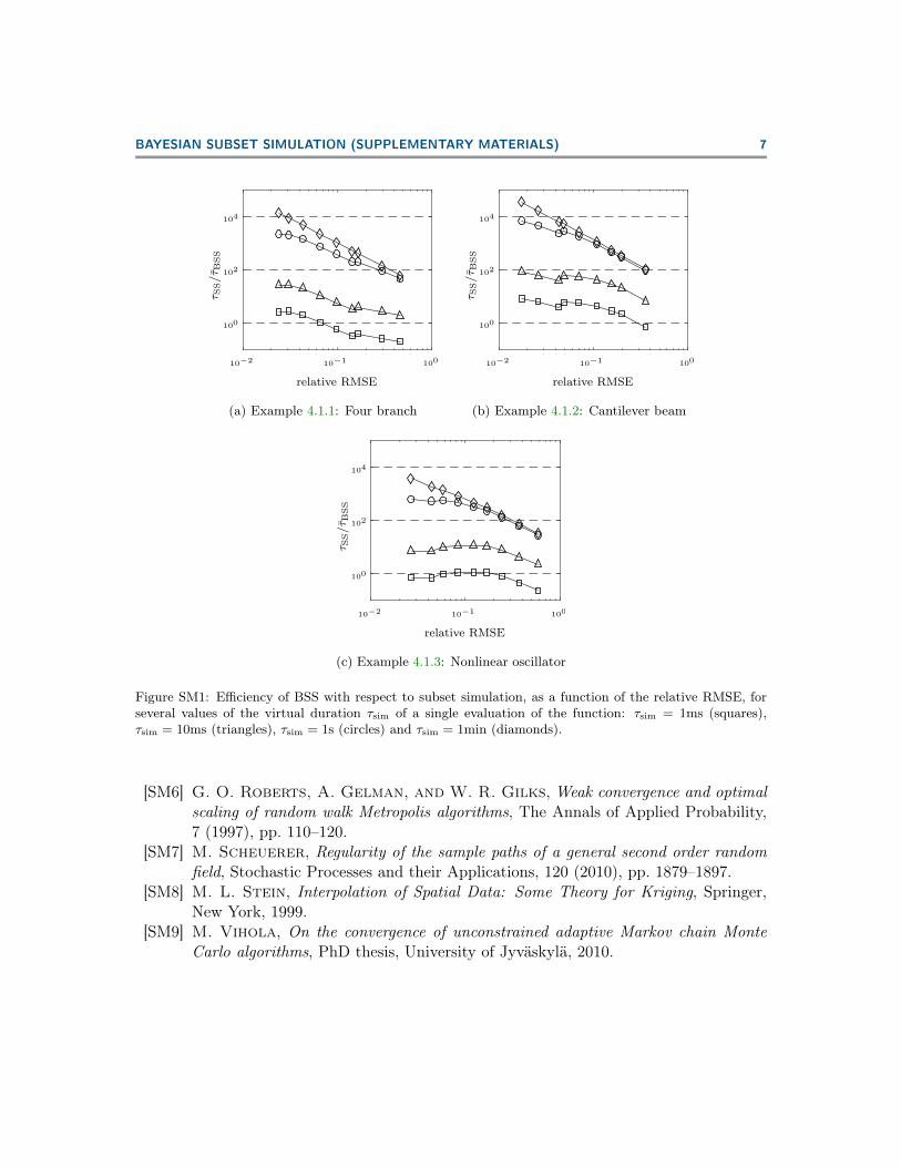
BAYESIAN SUBSET SIMULATION (SUPPLEMENTARY MATERIALS) 7
relative RMSE
τ SS/τ B
SS
10−2
10−1
100
100
102
104
(a) Example 4.1.1: Four branch
relative RMSE
τ SS/τ B
SS
10−2
10−1
100
100
102
104
(b) Example 4.1.2: Cantilever beam
relative RMSE
τ SS/τ B
SS
10−2
10−1
100
100
102
104
(c) Example 4.1.3: Nonlinear oscillator
Figure SM1: Efficiency of BSS with respect to subset simulation, as a function of the relative RMSE, forseveral values of the virtual duration τsim of a single evaluation of the function: τsim = 1ms (squares),τsim = 10ms (triangles), τsim = 1s (circles) and τsim = 1min (diamonds).
[SM6] G. O. Roberts, A. Gelman, and W. R. Gilks, Weak convergence and optimalscaling of random walk Metropolis algorithms, The Annals of Applied Probability,7 (1997), pp. 110–120.
[SM7] M. Scheuerer, Regularity of the sample paths of a general second order randomfield, Stochastic Processes and their Applications, 120 (2010), pp. 1879–1897.
[SM8] M. L. Stein, Interpolation of Spatial Data: Some Theory for Kriging, Springer,New York, 1999.
[SM9] M. Vihola, On the convergence of unconstrained adaptive Markov chain MonteCarlo algorithms, PhD thesis, University of Jyväskylä, 2010.