Banach and Hilbert Spaces MAP391/ MAPM91 - …math.swansea.ac.uk/staff/vm/BHS/banach-ln.pdf1.2...
40
Banach and Hilbert Spaces MAP391/ MAPM91 Lecture Notes 2008 – 2009 Vitaly Moroz Department of Mathematics Swansea University Singleton Park Swansea SA2 8PP Wales, UK [email protected]
-
Upload
truongdung -
Category
Documents
-
view
217 -
download
0
Transcript of Banach and Hilbert Spaces MAP391/ MAPM91 - …math.swansea.ac.uk/staff/vm/BHS/banach-ln.pdf1.2...
Banach and Hilbert SpacesMAP391/ MAPM91Lecture Notes 2008 – 2009
Vitaly Moroz
Department of MathematicsSwansea University
Singleton ParkSwansea SA2 8PP
Wales, [email protected]
Notations
N the set positive integers;
R field of real numbers;
C field of complex numbers;
Recommended Texts
The following books (amongst many others) could be recommended as a complementary readingfor this course:
1. L. Debnath, P. Mikusinski, Introduction to Hilbert spaces with applications. Second edition.Academic Press, Inc., San Diego, CA, 1999. xx+551 pp.
2. B. Rynne, M. Youngson, Linear functional analysis. Springer Undergraduate MathematicsSeries. Springer-Verlag London, Ltd., London, 2000. x+273 pp.
3. V. Hutson, J. Pym, M. Cloud, Applications of functional analysis and operator theory.Second edition. Mathematics in Science and Engineering, 200. Elsevier B. V., Amsterdam, 2005.xiv+426 pp.
The text of this Lecture Notes follows closely the content of the first chapters of [1] and theRussian textbook:
V. A. Trenogin, Functional analysis. (Russian) “Nauka”, Moscow, 1980. 496 pp.Unfortunately there is no English translation of this book.
Contents
1 Linear vector spaces 11.1 Linear vector spaces . . . . . . . . . . . . . . . . . . . . . . . . . . . . . . . . . . . 11.2 Linear combinations and linear dependence . . . . . . . . . . . . . . . . . . . . . . 21.3 Linear subspaces . . . . . . . . . . . . . . . . . . . . . . . . . . . . . . . . . . . . . 31.4 Dimension . . . . . . . . . . . . . . . . . . . . . . . . . . . . . . . . . . . . . . . . . 4
2 Normed spaces 52.1 Normed spaces . . . . . . . . . . . . . . . . . . . . . . . . . . . . . . . . . . . . . . 52.2 Spaces C([a, b]) and Ck([a, b]) . . . . . . . . . . . . . . . . . . . . . . . . . . . . . . 62.3 Spaces lp . . . . . . . . . . . . . . . . . . . . . . . . . . . . . . . . . . . . . . . . . . 72.4 Spaces Lp([a, b]) . . . . . . . . . . . . . . . . . . . . . . . . . . . . . . . . . . . . . 9
3 Analysis in Normed spaces 103.1 Convergence in normed spaces . . . . . . . . . . . . . . . . . . . . . . . . . . . . . 103.2 Cauchy sequences . . . . . . . . . . . . . . . . . . . . . . . . . . . . . . . . . . . . . 113.3 Bounded sets . . . . . . . . . . . . . . . . . . . . . . . . . . . . . . . . . . . . . . . 123.4 Open and closed sets . . . . . . . . . . . . . . . . . . . . . . . . . . . . . . . . . . . 133.5 Closure. Dense sets . . . . . . . . . . . . . . . . . . . . . . . . . . . . . . . . . . . . 143.6 Compact sets . . . . . . . . . . . . . . . . . . . . . . . . . . . . . . . . . . . . . . . 15
4 Banach spaces 174.1 Completeness property and Banach spaces . . . . . . . . . . . . . . . . . . . . . . . 174.2 Series in Banach spaces . . . . . . . . . . . . . . . . . . . . . . . . . . . . . . . . . 204.3 Completion of a normed space . . . . . . . . . . . . . . . . . . . . . . . . . . . . . 214.4 Banach spaces Lp([a, b]) . . . . . . . . . . . . . . . . . . . . . . . . . . . . . . . . . 22
5 Hilbert spaces 255.1 Inner product spaces . . . . . . . . . . . . . . . . . . . . . . . . . . . . . . . . . . . 255.2 Hilbert spaces. Orthogonal and orthonormal systems . . . . . . . . . . . . . . . . . 285.3 Fourier series . . . . . . . . . . . . . . . . . . . . . . . . . . . . . . . . . . . . . . . 315.4 Separable Hilbert spaces . . . . . . . . . . . . . . . . . . . . . . . . . . . . . . . . . 36
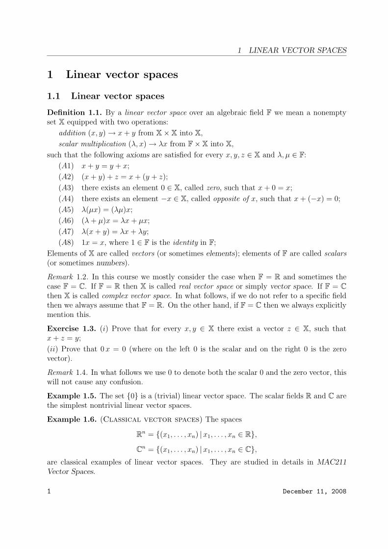
1 LINEAR VECTOR SPACES
1 Linear vector spaces
1.1 Linear vector spaces
Definition 1.1. By a linear vector space over an algebraic field F we mean a nonemptyset X equipped with two operations:
addition (x, y) → x + y from X× X into X,
scalar multiplication (λ, x) → λx from F× X into X,
such that the following axioms are satisfied for every x, y, z ∈ X and λ, µ ∈ F:
(A1) x + y = y + x;
(A2) (x + y) + z = x + (y + z);
(A3) there exists an element 0 ∈ X, called zero, such that x + 0 = x;
(A4) there exists an element −x ∈ X, called opposite of x, such that x + (−x) = 0;
(A5) λ(µx) = (λµ)x;
(A6) (λ + µ)x = λx + µx;
(A7) λ(x + y) = λx + λy;
(A8) 1x = x, where 1 ∈ F is the identity in F;
Elements of X are called vectors (or sometimes elements); elements of F are called scalars(or sometimes numbers).
Remark 1.2. In this course we mostly consider the case when F = R and sometimes thecase F = C. If F = R then X is called real vector space or simply vector space. If F = Cthen X is called complex vector space. In what follows, if we do not refer to a specific fieldthen we always assume that F = R. On the other hand, if F = C then we always explicitlymention this.
Exercise 1.3. (i) Prove that for every x, y ∈ X there exist a vector z ∈ X, such thatx + z = y;
(ii) Prove that 0 x = 0 (where on the left 0 is the scalar and on the right 0 is the zerovector).
Remark 1.4. In what follows we use 0 to denote both the scalar 0 and the zero vector, thiswill not cause any confusion.
Example 1.5. The set 0 is a (trivial) linear vector space. The scalar fields R and C arethe simplest nontrivial linear vector spaces.
Example 1.6. (Classical vector spaces) The spaces
Rn = (x1, . . . , xn) |x1, . . . , xn ∈ R,
Cn = (x1, . . . , xn) |x1, . . . , xn ∈ C,are classical examples of linear vector spaces. They are studied in details in MAC211Vector Spaces.
1 December 11, 2008
1.2 Linear combinations and linear dependence 1 LINEAR VECTOR SPACES
Example 1.7. (Function spaces) Let Ω be an arbitrary nonempty subset of Rn. Denoteby L(Ω) the set of all functions from Ω into R. Let x, y ∈ L(Ω) be functions and λ ∈ R ascalar. Define the addition and scalar multiplication in the natural pointwise way:
(x + y)(t) := x(t) + y(t),
(λx)(t) := λx(t).
Then L(Ω) becomes a linear vector space. Note that elements (vectors) of L(Ω) are func-tions from Ω into R. Linear vector spaces whose elements are functions are often calledfunction spaces.
In what follows we mostly consider the cases when Ω is an interval [a, b] of the real line,or Ω = R. Further examples of function spaces include:
C(Ω) – the space of all continuous real–valued functions on Ω;
Ck(Ω) – the space of all k–times continuously differentiable real–valued functions on Ω;
Pm(Ω) – the space of all real polynomials on Ω, of degree non greater then m;
P(Ω) – the space of all real polynomials on Ω.
Other examples of function spaces will be introduced later.
Exercise 1.8. Verify that the set L(Ω) with the natural pointwise addition and scalarmultiplication indeed satisfies axioms (A1− A8).
Example 1.9. (Spaces of sequences) Denote by l the set of all (infinite) sequencesof real numbers. Let x = (x1, x2, . . . ), y = (y1, y2, . . . ) ∈ l are sequences and λ ∈ R is ascalar. Define the addition and scalar multiplication in the natural way:
x + y := (x1 + y1, x2 + y2, . . . ),
λx := (λx1, λx2, . . . ).
Then l becomes a linear vector space. Note that elements (vectors) of l are sequences.Linear vector spaces whose elements are sequences are often called spaces of sequences.Further examples of function spaces include:
l∞ – the space of all bounded sequences of real numbers;
lc – the space of all convergent sequences of real numbers;
Other examples of spaces of sequences will be introduced later.
Exercise 1.10. Verify that the set L(Ω) with the natural pointwise addition and scalarmultiplication indeed satisfies axioms (A1− A8).
1.2 Linear combinations and linear dependence
Definition 1.11. Let X be a linear vector space and x1, . . . , xk ∈ X vectors. For givenscalars λ1, . . . , λk ∈ F, the vector λ1x1 + · · ·+λkxk is called a linear combination of vectorsx1, . . . , xk. The set of all linear combinations
λ1x1 + · · ·+ λkxk|λ1, . . . λk ∈ F
2 December 11, 2008
1.3 Linear subspaces 1 LINEAR VECTOR SPACES
is called (linear) span of vectors x1, . . . , xk and denoted spanx1, . . . , xk.Definition 1.12. Let X be a linear vector space. Vectors x1, . . . , xk ∈ X are called linearlyindependent if for any λ1, . . . , λk ∈ F
λ1x1 + · · ·+ λkxk = 0 =⇒ λ1 = · · · = λk = 0.
Otherwise, x1, . . . , xk ∈ X are called linearly dependent.
Example 1.13. Vectors x1 = (1, 0, 0), x2 = (0, 1, 0), x3 = (0, 0, 1) are linearly independentin R3. Vectors x1 = (1, 1, 0), x2 = (1,−1, 0), x3 = (1, 0, 0) are linearly dependent in R3, tosee this take λ1 = 1, λ2 = 1, λ3 = −2.
Example 1.14. Vectors x1(t) = sin2(t), x2(t) = cos2(t), x3(t) = 1 are linearly dependentin C([0, π]). To see this take λ1 = 1, λ2 = 1, λ3 = −1.
Exercise 1.15. Vectors x1(t) = 1, x2(t) = cos(2t), x3(t) = cos2(t) are linearly dependentin C([0, π]).
Hint. Use trigonometric identity cos(2t) = 2 cos2(t)− 1.
Exercise 1.16. Vectors x1(t) = 1, x2(t) = t, x3(t) = t2 are linearly independent in P(R).
Hint. Quadratic equation λ1 + λ2t + λ3t2 = 0 has no more then two real roots unless
λ1 = λ2 = λ3 = 0.
1.3 Linear subspaces
Definition 1.17. Let X be a linear vector space and L a subset of X. L is a linear subspaceof X if
for every x, y ∈ L and λ ∈ F one has λx ∈ L and x + y ∈ L.
Remark 1.18. It is easy to see that if L ⊂ X is a linear subspace of X then L is a linearvector space itself, with induced from X operations of addition and scalar multiplications.
Exercise 1.19. Fix A ∈ R. Let MA := x ∈ R3 |x1 + x2 + x3 = A. For which value(s)of A the set MA is a linear subspace of R3 ?
Example 1.20. The spaces P([a, b]), Ck([a, b]), C([a, b]) are linear subspaces of L([a, b]).In fact, for any integers k > l ≥ 0 we have the following sequence of embedded linearsubspaces:
P([a, b]) ⊂ Ck([a, b]) ⊂ C l([a, b]) ⊂ L([a, b]).
Example 1.21. The set M := x ∈ C([a, b]) |x(a) = 0, x(b) = 1 is not a linear subspaceof C([a, b]). To see this, simply observe that 0 6∈ M , so M is not a linear vector space,although M ⊂ C([a, b]).
Example 1.22. The space l∞ is a linear subspace of the space l.
Exercise 1.23. Fix A ∈ R. Let MA be the set of all sequences of real number whichconverge to A. Thus MA ⊂ l∞ (explain why!). For which value(s) of A the set MA is alinear subspace of l∞ ?
3 December 11, 2008
1.4 Dimension 1 LINEAR VECTOR SPACES
1.4 Dimension
Definition 1.24. Let X be a linear vector space. We say that X has dimension n ∈ Nand write dim X = n if:
i) there exists n linearly independent vectors x1, . . . , xn ∈ X;
ii) every n + 1 vectors y1, . . . , yn, yn+1 ∈ X are linearly dependent.
Remark 1.25. Properties (i) and (ii) together mean that X = span(x1, . . . , xn).
Example 1.26. The space Rn has dimension n. Indeed, it is known that Rn admits abasis e1, . . . , en so that:
i) vectors e1, . . . , en are linearly independent;
ii) every vector y ∈ Rn is represented as a linear combination of basis vectors.
This means that dim(Rn) = n.
Exercise 1.27. Show that the space Pm(R) of all real polynomials of degree non greaterthen m has dimension m.
Definition 1.28. Let X be a linear vector space. We say that X has infinite dimensionand write dim X = ∞ if for every k ∈ N there exists k linearly independent vectorsx1, . . . , xk ∈ X.
Example 1.29. The space l∞ is infinite dimensional. To see this, define
e1 := (1, 0, 0, 0, 0, . . . ),
e2 := (0, 1, 0, 0, 0, . . . ),
e3 := (0, 0, 1, 0, 0, . . . ),
. . .
It is easy to see that for every k ∈ N vectors e1, . . . , ek ∈ l∞ are linearly independent.
Exercise 1.30. Prove that the space of all polynomials P([a, b]) is infinite dimensional.
Hint. Show that for all k ∈ N vectors
x1(t) = 1, x2(t) = t, . . . , xk(t) = tk−1,
are linearly independent in P([a, b]). To do this, use Fundamental Theorem of Algebraabout the roots of polynomials of degree k.
Exercise 1.31. Use previous exercise to conclude that the space C([a, b]) and the spacesCk([a, b]) are infinite dimensional.
4 December 11, 2008
2 NORMED SPACES
2 Normed spaces
2.1 Normed spaces
Definition 2.1. Let X be a linear vector space. A norm on X is a function ‖ · ‖ : X →[0, +∞) such that the following axioms are satisfied for all x, y ∈ X and λ ∈ F:
(N1) ‖x‖ = 0 implies x = 0.
(N2) ‖λx‖ = |λ|‖x‖;(N3) ‖x + y‖ ≤ ‖x‖+ ‖y‖ (triangle inequality).
A normed space is a pair (X, ‖ · ‖), where X is a linear vector space and ‖ · ‖ is a norm onX.
Remark 2.2. For x ∈ X, the number ‖x‖ is called the norm of ‖x‖ and has a geometricalmeaning of the ”length” of the vector x.
Exercise 2.3. Let X be a normed space with the norm ‖ · ‖. Prove that for any x, y ∈ Xthe following useful inequality holds:
(2.1) |‖x‖ − ‖y‖| ≤ ‖x− y‖.
Example 2.4. The function ‖x‖ :=√|x1|2 + · · ·+ |xn|2 defines the Euclidean norm on
Rn.
Example 2.5. It is possible to define different norms on the same linear vector space. Forinstance, for p ∈ [1,∞) the function
‖x‖p := p√|x1|p + · · ·+ |xn|p
defines a norm on Rn, which is often called p-norm. Indeed, axioms (N1) and (N2) for ‖·‖p
are obvious, while the triangle inequality (N3) is nothing else but Minkowski’s inequality1,which states that for every x, y ∈ Rn one has
(2.2)
(n∑
i=1
|xi + yi|p)1/p
≤
(n∑
i=1
|xi|p)1/p
+
(n∑
i=1
|yi|p)1/p
.
Observe, that the Euclidean norm on Rn is just a particular case of the p-norm with p = 2.
Exercise 2.6. Prove that the function
‖x‖∞ := max|x1|, . . . , |xn|
defines a norm on Rn. This norm is often called infinity norm.
Notation 2.7. For p ∈ [1,∞], Rnp denotes the space Rn equipped with the norm ‖ · ‖p.
However if p = 2 then the subscript is often omitted.
1Minkowski’s inequality was proved in Analysis 2.
5 December 11, 2008

2.2 Spaces C([a, b]) and Ck([a, b]) 2 NORMED SPACES
2.2 Spaces C([a, b]) and Ck([a, b])
Let C([a, b]) be the space of all continuous functions on the closed interval [a, b]. Thefunction
(2.3) ‖x‖∞ := maxt∈[a,b]
|x(t)|
defines a norm on the space C([a, b]). Indeed, every continuous function on the closedinterval [a, b] attains its maximum (this is Weierstrass Theorem from Analysis). Therefore,‖x‖∞ is well defined and nonnegative for every x ∈ C([a, b]). Verification of axioms (N1)and (N2) of the norm is elementary. To verify (N3) observe that
|x(t) + y(t)| ≤ |x(t)|+ |y(t)| ≤ maxt∈[a,b]
|x(t)|+ maxt∈[a,b]
|y(t)| (t ∈ [a, b]).
Hence
‖x + y‖∞ = maxt∈[a,b]
|x(t) + y(t)| ≤ maxt∈[a,b]
|x(t)|+ maxt∈[a,b]
|y(t)| = ‖x‖∞ + ‖y‖∞,
which proves the triangle inequality (N3).
Notation 2.8. In what follows C([a, b]) always denotes the normed space of all continuousfunctions on the closed interval [a, b], with the norm ‖ · ‖∞.
For k ∈ N, let Ck([a, b]) be the space of all k–times continuously differentiable functionson the closed interval [a, b]. The function
(2.4) ‖x‖∞,k := maxt∈[a,b]
|x(t)|+ maxt∈[a,b]
|x′(t)|+ · · ·+ maxt∈[a,b]
|x(k)(t)|
defines a norm on Ck([a, b]).
Exercise 2.9. Verify, that the function ‖ · ‖∞,k indeed satisfies axioms of the norm (N1−N3).
Notation 2.10. In what follows Ck([a, b]) always denotes the normed space of all k–timescontinuously differentiable functions on the closed interval [a, b], with the norm ‖ · ‖∞,k.
Exercise 2.11. Let C(R) be the space of all continuous functions on the real line. Explainwhy
‖x‖ := maxt∈R
|x(t)|
does not define a norm on C(R).
Hint. Is this norm finite for every x ∈ C(R) ?
Exercise 2.12. Let C1([a, b]) be the space of all continuously differentiable functions onthe interval [a, b]. Explain why
‖x‖ := maxt∈R
|x′(t)|
does not define a norm on C1([a, b]).
Hint. Check property (N1) of the norm.
6 December 11, 2008

2.3 Spaces lp 2 NORMED SPACES
2.3 Spaces lp
Definition 2.13. Denote by lp, for p ≥ 1, the space of all sequences x = (x1, x2, . . . ) ofreal numbers, such that
‖x‖p :=
(∞∑i=1
|xi|p)1/p
< ∞.
To prove that lp is a normed space we will need a version of Minkowski’s inequality forinfinite sequences.
Lemma 2.14. (Minkowski inequality for sequences) Let p ≥ 1. For all x, y ∈ lpone has
(2.5)
(∞∑i=1
|xi + yi|p)1/p
≤
(∞∑i=1
|xi|p)1/p
+
(∞∑i=1
|yi|p)1/p
.
Proof. Let x, y ∈ lp and let n ∈ N. In the right hand side of the Minkowski’s inequalityfor finite sums (2.2), we can replace n by any integer m ≥ n, so(
n∑i=1
|xi + yi|p)1/p
≤
(m∑
i=1
|xi|p)1/p
+
(m∑
i=1
|yi|p)1/p
.
Passing to the limit as m →∞ in the above inequality, we conclude that(n∑
i=1
|xi + yi|p)1/p
≤
(∞∑i=1
|xi|p)1/p
+
(∞∑i=1
|yi|p)1/p
.
Since n in the left hand side of the above inequality is arbitrary, we conclude that the seriesin left hand side converges (as the series with nonnegative terms and uniformly boundedpartial sums). Passing to the limit as n →∞ we obtain (2.5).
Remark 2.15. Minkowski’s inequality for sequences can be rewritten simply as
‖x + y‖p ≤ ‖x‖p + ‖y‖p.
Proposition 2.16. (lp, ‖ · ‖p) is a normed space.
Proof. To prove that (lp, ‖ · ‖p) is a normed space we first need to show that lp is a linearvector space. Since lp ⊂ l, it is enough to verify that lp is a linear subspace of l, that is:
x, y ∈ lp and λ ∈ R implies that λx ∈ lp and x + y ∈ lp.
Further, we need to show that ‖ · ‖p satisfies axioms of the norm (N1−N3).
7 December 11, 2008

2.3 Spaces lp 2 NORMED SPACES
Assume that x, y ∈ lp and λ ∈ R. We first observe that
‖λx‖p = |λ|‖x‖p < ∞,
which shows that λx ∈ lp and also proves (N2). Further, from Minkowski’s inequality (2.5)we conclude that
‖x + y‖p ≤ ‖x‖p + ‖y‖p,
which shows that x + y ∈ lp and also proves (N3). Finally, axiom (N1) of the norm isobvious. This completes the proof.
Definition 2.17. Denote by l∞ the normed space of all bounded sequences x = (x1, x2, . . . )of real numbers, with the norm
‖x‖∞ := maxi∈N
|xi|.
Exercise 2.18. Verify that (l∞, ‖ · ‖∞) is a normed space.
Notation 2.19. To simplify the notations, in what follows lp always denotes the normedspace (lp, ‖ · ‖p) (p ∈ [1,∞]).
Exercise 2.20. Show that if p 6= q then lp 6= lq.
Hint. Consider the sequence xk = 1/ka (k ∈ N). For which values of a ≥ 0 the sequence(xk) belongs to lp ?
Exercise∗ 2.21. Let p, q ∈ [1,∞] and p < q. Prove that
lp ⊂ lq.
Definition 2.22. Let p ∈ [1,∞]. The conjugate to p is the number p′ such that
(2.6)1
p+
1
p′= 1.
We agree that if p = 1 then p′ = ∞, and if p = ∞ then p′ = 1.
Lemma 2.23. (Holder inequality for sequences2) Let p ∈ [1, +∞]. Let x ∈ lp andy ∈ lp′, where p′ is the conjugate to p. Then
(2.7)∞∑i=1
|xiyi| ≤ ‖x‖p‖y‖p′ .
Exercise 2.24. Derive Holder’s inequality for sequences from Holder’s inequality for finitesums in a way, similar to the proof of Lemma 2.14.
2Holder’s inequality for finite sums was proved in Analysis 2
8 December 11, 2008
2.4 Spaces Lp([a, b]) 2 NORMED SPACES
2.4 Spaces Lp([a, b])
Definition 2.25. Denote by Lp([a, b]), for p ≥ 1, the space of all continuous functionsx : [a, b] → R with the norm
‖x‖p :=
(∫ b
a
|x(t)|p dt
)1/p
< ∞,
where the integral in the right hand side is understood in the Riemann sense.
To prove that Lp([a, b]) is a normed space we will need a version of Minkowski’s in-equality for Riemann integrals.
Lemma 2.26. (Minkowski inequality for Riemann integrals3) Let p ≥ 1. Forall continuous function x, y : [a, b] → R one has
(2.8)
(∫ b
a
|x(t) + y(t)|p dt
)1/p
≤(∫ b
a
|x(t)|p dt
)1/p
+
(∫ b
a
|y(t)|p dt
)1/p
.
Remark 2.27. Integral Minkowski’s inequality can be rewritten as
‖x + y‖p ≤ ‖x‖p + ‖y‖p.
Proposition 2.28. (Lp([a, b]), ‖ · ‖p) is a normed space.
Proof. To verify that ‖ · ‖p is indeed a norm observe that if x(t) is continuous function on[a, b] then |x(t)|p is also continuous, and hence, Riemann integrable on [a, b]. Therefore,‖x‖p is well defined, moreover it is nonnegative for every x ∈ C([a, b]). Verification ofaxioms (N1) and (N2) is elementary and is left as an exercise, while the triangle inequality(N3) is nothing else but Minkowski’s inequality for integrals
Remark 2.29. Observe that Lp([a, b]) contains the same collection of function as C([a, b]),however the norms in Lp([a, b]) and C([a, b]) are different.
Remark 2.30. The space C([a, b]) with the usual norm ‖·‖∞ can be interpreted as L∞([a, b])if we consider the maximum norm ‖ · ‖∞ as the ”limit” of integral p-norms when p →∞.Such interpretation will be further justified later in this course.
Lemma 2.31. (Holder inequality for integrals4) Let p > 1. Let x ∈ Lp([a, b])and y ∈ Lp′([a, b]), where p′ is the conjugate to p. Then
(2.9)
∫ b
a
|x(t)y(t)| dt ≤ ‖x‖p‖y‖p′ .
Exercise∗ 2.32. Let p, q ∈ [1,∞] and p < q. Prove that
Lq([a, b]) ⊂ Lp([a, b]).
Hint. Use Holder’s inequality for integrals.
3Minkowski’s inequality for integrals was proved in Analysis 24Holder’s inequality for integrals was proved in Analysis 2
9 December 11, 2008

3 ANALYSIS IN NORMED SPACES
3 Analysis in Normed spaces
3.1 Convergence in normed spaces
Definition 3.1. Let (X, ‖ · ‖) be a normed space and (xn) ⊂ X be a sequence of vectorsin X. We say that the sequence (xn) converges to a vector x ∈ X and write
limn→∞
xn = x or xn → x
iflim
n→∞‖xn − x‖ = 0.
In other words, this means that for every ε > 0 there exists N = N(ε) ∈ N such that forall integers n ≥ N one has
‖xn − x‖ < ε.
Remark 3.2. The limit of a convergent sequence is unique. Indeed, assume that (xn)converges to x ∈ X and y ∈ X. Then using the triangle inequality we obtain
‖x− y‖ = ‖(x− xn) + (xn − y)‖ ≤ ‖xn − x‖+ ‖xn − y‖ → 0.
Since the right hand side gets arbitrary small, we conclude that ‖x − y‖ = 0 and hencex = y.
Exercise 3.3. Let (X, ‖ · ‖) be a normed space, (xn), (yn) ⊂ X sequences of vectors in Xand (λn) ⊂ F a sequence of scalars. Prove the following properties of convergent sequences:
(i) if xn → x and λn → λ then λnxn → λx;
(ii) if xn → x and yn → y then xn + yn → x + y.
(iii) if xn → x then ‖xn‖ → ‖x‖
Hint. To prove (iii), use (2.1).
Example 3.4. (Convergence in C([a, b])) According to Definition 3.1, a sequence(xn) ⊂ C([a, b]) converges to x ∈ C([a, b]) if
‖xn − x‖∞ → 0.
This means that for every ε > 0 there exists N = N(ε) ∈ N such that for all integersn ≥ N one has
‖xn − x‖∞ = maxt∈[a,b]
|xn(t)− x(t)| < ε.
Thus convergence in C([a, b]) coincides with the uniform convergence which is studied Anal-ysis. For this reason, the norm ‖x‖∞ = maxt∈[a,b] |x(t)| is often called uniform convergencenorm.
10 December 11, 2008

3.2 Cauchy sequences 3 ANALYSIS IN NORMED SPACES
Exercise 3.5. Let xn(t) := ntn. Show that:
(i) The sequence (xn) converges to x(t) = in C([0, 1/2]);
(ii) The sequence (xn) has no limit in C([0, 1]).
Hint. To prove (ii), use Exercise 3.3 (iii).
Example 3.6. (Relation between convergences in C([a, b]) and Lp([a, b]) Con-sider a sequence of continuous functions xn : [a, b] → R (n ∈ N). Thus (xn) ⊂ C([a, b])and (xn) ⊂ Lp([a, b]). Assume that xn → x in C([a, b]). Then
‖xn − x‖p =
(∫ b
a
|xn(t)− x(t)|p dt
)1/p
≤(
maxt∈[a,b]
|xn(t)− x(t)|p(b− a)
)1/p
= (b− a)1/p‖xn − x‖∞ → 0.
Thus, we proved that if a sequence (xn) converges to x in C([a, b]) then for every p ∈ [1,∞)the sequence (xn) converges to the same limit x in Lp([a, b]).
Exercise 3.7. Consider the sequence
(3.1) xn(t) :=
sin(nt), t ∈ [0, π/n];
0, t ∈ [π/n, π].
Clearly (xn) ⊂ C([0, π]) and (xn) ⊂ Lp([0, π]) for any p ≥ 1. Prove that xn → 0 inLp([0, π]) for any p ≥ 1, but (xn) has no limit in C([0, π]). This shows, in particular, thatconvergence in Lp([0, π]) does not imply converges in C([0, π]).
Exercise∗ 3.8. Let p > q ≥ 1. Construct an example of a sequence (xn) which convergesto zero in Lp([0, π]) but does not have a limit in Lq([0, π]).
Hint. Consider sequences of the form yn(t) := Anxn(t), where xn(t) are functions from(3.1) and An > 0, then determine appropriate coefficients Ak.
Exercise∗∗ 3.9. (Relation between convergences in l1 and l∞) Consider a se-quence (xn) ⊂ l1. Prove that if (xn) converges to x in l1 then (xn) converges to the samelimit x in l∞.
Construct an example of a sequence (xn) which converges to zero in l∞ but does nothave a limit in l1.
3.2 Cauchy sequences
Definition 3.10. Let (X, ‖ · ‖) be a normed space and (xn) ⊂ X be a sequence of vectorsin X. We say that (xn) is a Cauchy sequence if for every ε > 0 there exists a positiveinteger N = N(ε) ∈ N such that for all positive integers n ≥ N and m ≥ N one has
‖xn − xm‖ < ε.
11 December 11, 2008
3.3 Bounded sets 3 ANALYSIS IN NORMED SPACES
Exercise 3.11. Show that if (xn) ⊂ X is a Cauchy sequence then the sequence of norms(‖xn‖) ⊂ R is a Cauchy sequence of real numbers. Give an example, showing that theopposite is not true.
Theorem 3.12. Let (X, ‖ · ‖) be a normed space and (xn) ⊂ X be a sequence. If thesequence (xn) converges then (xn) is a Cauchy sequence.
Proof. Let x := limn→∞ xn. Fix ε > 0. Then, according to Definition 3.1,
(∃N ∈ N)(∀n ∈ N)[(n ≥ N) ⇒ (‖xn − x‖ <ε
2)].
Let m, n ≥ N . By the triangle inequality (N3) we obtain
‖xn − xm‖ ≤ ‖xn − x‖+ ‖xm − x‖ < ε.
Therefore (xn) is a Cauchy sequence.
Exercise 3.13. Show that the sequence xn(t) := sin(nt) (n ∈ N) is not a Cauchy sequencein C([0, π]). Conclude from this that (xn) has no limit in C([0, π]). (This shows, inparticular, that the converse to Exercise 3.3 (iii) is not true.)
3.3 Bounded sets
Definition 3.14. Let (X, ‖ · ‖) be a normed space. We define:
BR(x) := y ∈ X | ‖y − x‖ < R – open ball of radius R > 0, centered at x ∈ X;
BR(x) := y ∈ X | ‖y − x‖ ≤ R – closed ball of radius R > 0, centered at x ∈ X;
SR(x) := y ∈ X | ‖y − x‖ = R – sphere of radius R > 0, centered at x ∈ X.
Exercise 3.15. Draw a picture of B1(0), B1(0), S1(0) in: (R2, ‖·‖2); (R2, ‖·‖1); (R2, ‖·‖∞).
Exercise 3.16. Try to illustrate how B1(0) looks like in: C([0, 1]); Lp([0, 1]).
Definition 3.17. Let (X, ‖ · ‖) be a normed space and M ⊂ X a nonempty subset of X.We say that the set M is bounded in X if there exists R > 0 such that M ⊂ BR(0). Inother words, this means that there exists R > 0 such that ‖x‖ < R, for every x ∈ M . If aset M is not bounded then it is said to be unbounded.
Theorem 3.18. Let (X, ‖ · ‖) be a normed space and (xn) ⊂ X be a sequence. If thesequence (xn) converges then (xn) is bounded.
Proof. Let x := limn→∞ xn. By the triangle inequality (N3) we have
‖xn‖ = ‖(xn − x) + x‖ ≤ ‖xn − x‖+ ‖x‖.
12 December 11, 2008
3.4 Open and closed sets 3 ANALYSIS IN NORMED SPACES
Note that the sequence of real numbers (‖xn − x‖) converges to zero. It is known fromAnalysis that every convergent sequence of real numbers is bounded. Hence the sequenceof real numbers (‖xn − x‖) is bounded, that is there exists C > 0 such that
(∀n ∈ N)[‖xn − x‖ < C].
Therefore by the triangle inequality
(∀n ∈ N)[‖xn‖ ≤ ‖xn − x‖+ ‖x‖ ≤ C + ‖x‖],
which means that (xn) ⊂ BC+‖x‖(0) and hence (xn) is bounded.
Example 3.19. The converse to Theorem 3.18 in generally is not true in normed spaces.To see this consider the sequence xn(t) := sin(nt) (n ∈ N) in C([0, π]). The sequence (xn)has no limit in C([0, π]). However, ‖xn‖∞ = 1, so (xn) is bounded in C([0, π])!
3.4 Open and closed sets
Definition 3.20. Let (X, ‖ · ‖) be a normed space and M ⊂ X a nonempty subset ofX. We say that the set M is open in X if for every x ∈ M there exists R > 0 such thatBR(x) ⊂ M . A subset M is closed if its complement is open, that is if X \M is open.
Remark 3.21. There are sets which are neither open nor closed. For instance, the interval[0, 1) ⊂ R is neither open nor closed in R!
Example 3.22. Open ball BR(x) in a normed space X is an open set. Closed ball BR(x)and sphere SR(x) are closed sets.
Example 3.23. For a given function x ∈ C([a, b]), the following set are open in C([a, b]) :
y ∈ C([a, b]) | y(t) < x(t) for all t ∈ [a, b],
y ∈ C([a, b]) | y(t) > x(t) for all t ∈ [a, b],
y ∈ C([a, b]) | |y(t)| < x(t) for all t ∈ [a, b],
y ∈ C([a, b]) | |y(t)| > x(t) for all t ∈ [a, b].
The following sets are closed in C([a, b]) :
y ∈ C([a, b]) | y(t) ≤ x(t) for all t ∈ [a, b],
y ∈ C([a, b]) | y(t) ≥ x(t) for all t ∈ [a, b],
y ∈ C([a, b]) | |y(t)| ≤ x(t) for all t ∈ [a, b],
y ∈ C([a, b]) | |y(t)| ≥ x(t) for all t ∈ [a, b].
13 December 11, 2008
3.5 Closure. Dense sets 3 ANALYSIS IN NORMED SPACES
Theorem 3.24. (Properties of open and closed sets)
(i) The union of any collection of open sets is open.
(ii) The intersection of a finite number of open sets is open.
(iii) The union of a finite number of closed sets is closed.
(iv) The intersection of any collection of closed sets is closed.
(v) The empty set and the whole space are both open and closed.
Proof. Prove these properties as an exercise (see also Analysis 3).
Theorem 3.25. Let (X, ‖ · ‖) be a normed space and M ⊂ X a nonempty subset of X. Mis closed if and only if every convergent sequence of elements in M has its limit in M , thatis
(xn) ⊂ M and xn → x implies x ∈ M.
Proof. Let M be a closed subset of X and (xn) ⊂ X a sequence in X such that xn → x.Suppose that x 6∈ M . Since M is closed, X \M is open. Then there exists ε > 0 such thatBε(x) ⊂ X\M . On the other hand, since xn → x we have ‖xn−x‖ < ε for all large n ∈ N.But (xn) ⊂ M ! This contradictions shows that x ∈ M .
Now suppose that
(xn) ⊂ M and xn → x implies x ∈ M.
If M is not closed then X \M is not open. Thus there exists x ∈ X \M such that everyball Bε(x) contains elements of M . Thus, we can find (xn) ⊂ M such that xn ∈ B1/n(x).But then xn → x and according to our assumption, x ∈ M . Therefore M must be a closedset!
3.5 Closure. Dense sets
Definition 3.26. Let (X, ‖ · ‖) be a normed space and M ⊂ X a nonempty subset of X.The closure of the set M is the of limits of all convergent sequences of elements of M , i.e.
clM := x ∈ X | there exists (xn) ⊂ M such that xn → x.
Remark 3.27. It is clear that if a set M is closed then clM = M . One can show that theclosure of a set M is the ”smallest” closed set which contains M .
Example 3.28. Let X = R. Then cl(0, 1) = [0, 1] and clQ = R.
Definition 3.29. Let (X, ‖ · ‖) be a normed space and M ⊂ X a nonempty subset of X.The set M is dense in X if clM = X.
Example 3.30. The set of rationals Q is dense in R.
Example 3.31. (Weiertrass Theorem) The Weierstrass theorem says that every con-tinuous function on an interval [a, b] can be uniformly approximated by polynomials. Thiscan be interpreted as follows: the space of polynomials P([a, b]) is dense in C([a, b]).
14 December 11, 2008

3.6 Compact sets 3 ANALYSIS IN NORMED SPACES
3.6 Compact sets
Definition 3.32. Let (X, ‖ · ‖) be a normed space and M ⊂ X a nonempty subset ofX. The set M is compact if every sequence (xn) ⊆ M contain a subsequence (xnk
) whichconverges in M , that is xnk
→ x ∈ M .
Example 3.33. Every bounded and closed subset of Rn is compact. In particular, theclosed unit ball in RN is compact.
Theorem 3.34. Let (X, ‖ · ‖) be a normed space and M ⊂ X a nonempty subset of X. IfM is compact then M is bounded and closed.
Proof. Suppose (xn) ⊆ M and xn → x. Since M is compact, (xn) contain a convergentsubsequence xnk
such that xnk→ y ∈ M . On the other hand, we have xn → x. Thus
x = y and x ∈ M . By Theorem 3.25 we conclude that M is closed.
Assume that M is unbounded. Then for every m ∈ N there exists xm ∈ M such that‖xm‖ ≥ m. In such a way, we constructed a sequence (xm) ⊂ M which is unbounded.Clearly, (xm) can not contain a convergent subsequence (cf. Theorem 3.18). Hence M isnot compact.
Example 3.35. (The unit ball in C([0, 1]) is non compact) Consider the sequencexn(t) := tn (n ∈ N). Clearly (xn) ⊂ C([0, 1]) and ‖xn‖∞ = 1, so (xn) belongs to the closedunit ball B1(0) ⊂ C([0, 1]). Since convergence in C([0, 1]) coincides with the uniformconvergence, we conclude that the sequence (xn) does not have a convergent subsequencein C([0, 1]). Therefore, the unit ball in C([0, 1]) is not compact.
Theorem 3.36. A normed space X is infinite dimensional if and only if the closed unitball in X is not compact.
Proof. A special case of this theorem will be proved later. For the full proof see, e.g.[1,2].
Equivalent norms5
Definition 3.37. Let (X, ‖ · ‖1) and (X, ‖ · ‖2) be normed spaces. The norms ‖ · ‖1 and ‖ · ‖2 arecalled equivalent if there exist α, β ∈ R, β ≥ α > 0, such that for all x ∈ X one has
(3.2) α‖x‖1 ≤ ‖x‖2 ≤ β‖x‖2.
Exercise 3.38. Show that the following norms on R2 are equivalent:
‖x‖1 = |x1|+ |x2|, ‖x‖2 =√|x1|2 + |x2|2, ‖x‖∞ = max|x1|, |x2| (x = (x1, x2) ∈ R2).
5Optional
15 December 11, 2008
3.6 Compact sets 3 ANALYSIS IN NORMED SPACES
Theorem 3.39. Let (X, ‖ · ‖1) and (X, ‖ · ‖2) be normed spaces. The norms ‖ · ‖1 and ‖ · ‖2 onX are equivalent if and only if for any sequence (xn) ⊂ X and any x ∈ X one has
‖xn − x‖1 → 0 ⇐⇒ ‖xn − x‖2 → 0.
Proof. See [2,Theorem 1.3.11].
Remark 3.40. The above theorem tells that two norms on the same linear vector space are equiv-alent if they define the same convergence, and therefor the same classes of convergent sequences,Cauchy sequences, open and closed sets, compact sets etc. Effectively, this means that Analysisin normed spaces with equivalent norms is essentially identical.
Example 3.41. Exercises 3.7 and 3.8 show that the norms of C([a, b]) and Lp([a, b]), and ofLp([a, b]) and Lq([a, b]) with p 6= q, are not equivalent.
Theorem 3.42. Let X be a finite dimensional linear vector space. Then any two norms on Xare equivalent.
Proof. See [2,Theorem 1.3.13].
Remark 3.43. The above theorem tells that Analysis in finite dimensional spaces essentially doesnot depend on the choice of a particular norm.
16 December 11, 2008
4 BANACH SPACES
4 Banach spaces
4.1 Completeness property and Banach spaces
Recall that every convergent sequence in a normed space is a Cauchy sequence, see Theorem3.12. The converse is not true, in general.
Example 4.1. Let P([0, 1]) be the normed space of polynomials on [0, 1] with the norm‖x‖∞ = maxt∈[0,1] |x(t)|. Define
xn(t) := 1 + t +t2
2!+ · · ·+ tn
n!,
for n ∈ N. Then (xn) is a Cauchy sequence in P([0, 1]), but it does not converge in P([0, 1])because its pointwise limit is the exponential function x(t) = et, which not a polynomial.
Definition 4.2. Let (X, ‖ · ‖) be a normed space. We say that X is complete if everyCauchy sequence (xn) ⊂ X converges to the limit in X. A complete normed space is calledBanach space.
Remark 4.3. According to the above example, the space P([0, 1]) is not complete.
Example 4.4. (Rnp is a Banach space) It is proved in Analysis that a sequence in Rn
converges if and only if it is a Cauchy sequence. This means that the spaces Rnp are Banach
spaces, for all p ∈ [1,∞].
Theorem 4.5. lp is a Banach space.
Proof. We give the proof for 1 ≤ p < ∞. Let (xn) be a Cauchy sequence in lp, and denote
xn = (χn,1, χn,2, . . . ).
Then for any ε > 0 there exists N ∈ N such that for all integers m, n > N one has
(4.1)∞∑
k=1
|χm,k − χn,k|p < εp.
This implies that for every fixed k ∈ N and for every ε > 0 there exists N0 ∈ N such thatfor all integers m, n > N0 one has
|χm,k − χn,k| < ε.
But this means that for every fixed k ∈ N the sequence of real numbers (χn,k) is a Cauchysequence in R and thus converges to a limit in R. Denote
χk := lim χn,k and χ := (χ1, χ2, . . . ).
17 December 11, 2008
4.1 Completeness property and Banach spaces 4 BANACH SPACES
We are going to show that χ ∈ lp and that xn converges to χ in lp.
Indeed, by letting m →∞ in (4.1), for every integer n ≥ N0 we obtain
(4.2)∞∑
k=1
|χk − χn,k|p < εp.
Since∞∑
k=1
|χN0,k|p < ∞,
by Minkowski’s inequality we have(∞∑
k=1
|χk|p)1/p
=
(∞∑
k=1
(|χk| − |χN0,k|+ |χN0,k|)p
)1/p
≤
(∞∑
k=1
(|χk| − |χN0,k|)p
)1/p
+
(∞∑
k=1
|χN0,k|p)1/p
≤
(∞∑
k=1
|χk − χN0,k|p)1/p
+
(∞∑
k=1
|χN0,k|p)1/p
< ∞.
This proves that χ ∈ lp. Moreover, since ε > 0 is arbitrary small, (4.2) implies that
lim ‖χ− χn‖p = lim
(∞∑
k=1
|χk − χN0,k|p)1/p
= 0,
which means that χn → χ in lp.
Exercise 4.6. Prove that l∞ is a Banach space.
Theorem 4.7. C([a, b]) is a Banach space.
Proof. Let (xn) be a Cauchy sequence in C([a, b]). Then for any ε > 0 there exists N ∈ Nsuch that for all integers m, n ≥ N one has
‖xn − xm‖∞ < ε,
or, in in other words, for all t ∈ [a, b] one has
(4.3) |xn(t)− xm(t)| < ε.
This, in particular, implies that for every fixed t ∈ [a, b] the sequence (xn(t)) is a Cauchysequence of real numbers and therefore (xn(t)) converges in R. Denote the limit of (xn(t))by x(t), so
x(t) := lim xn(t) (t ∈ [a, b]).
18 December 11, 2008
4.1 Completeness property and Banach spaces 4 BANACH SPACES
We are going to show that x ∈ C([a, b]) and that xn converges to χ in C([a, b]).
Indeed, by letting m →∞ in (4.3), for all integers n ≥ N and all t ∈ [a, b] we obtain
(4.4) |xn(t)− x(t)| < ε.
Let t0 ∈ [a, b]. Since xN is continuous on [a, b], there exists δ > 0 such that for all s ∈ [a, b]such that |s− t0| < δ one has
|xN(s)− xN(t0)| < ε.
Then
|x(s)− x(t0)| ≤ |x(s)− xN(s)|︸ ︷︷ ︸<ε
+ |xN(s)− xN(t0)|︸ ︷︷ ︸<ε
+ |xN(t0)− xN(t0)|︸ ︷︷ ︸<ε
< 3ε,
which proves continuity of x. Finally, (4.4) implies that for all integers n ≥ N we have
‖xn − x‖∞ ≤ ε,
which means that xn → x in C([a, b]).
Theorem 4.8. Lp([a, b]) is not complete.
Proof. We present the proof for p = 2. Consider the sequence of continuous functions(xn) ⊂ L2([−1, 1]), defined by
xn(t) :=
−1, t ∈ [−1,−1/n],nt t ∈ [−1/n, 1/n],1, t ∈ [1/n, 1].
It is clear that |xn(t)| ≤ 1 for all t ∈ [−1, 1] and hence |xn(t)−xm(t)| ≤ 2 for all t ∈ [−1, 1].Therefore, we compute
‖xm − xm‖2 =
∫ 1
−1
|xm(t)− xn(t)|2 dt ≤ 4
∫ 1/n
−1/n
dt =8
n→ 0.
Hence, (xn) is a Cauchy sequence in L2([−1, 1]). However, the ”limit” function
x(t) :=
−1, t ∈ [−1, 0),0 t = 0,1, t ∈ (0, 1].
is discontinuous and does not belong to the space L2([−1, 1]).
Exercise 4.9. Show that Lp([a, b]) is incomplete for any p ∈ [1,∞).
19 December 11, 2008
4.2 Series in Banach spaces 4 BANACH SPACES
4.2 Series in Banach spaces
Definition 4.10. Let (X, ‖ · ‖) be a normed space and (xk) ⊂ X be a sequence. A series
∞∑k=1
xk
is called convergent in X if the sequence of partial sums
Sn := x1 + x2 + · · ·+ xn
converges in X, that is there exists x ∈ X such that
‖Sn − x‖ → 0.
In this case we write∞∑
k=1
xk = x.
If the series of norms of the sequence (xn) converges, that is
∞∑k=1
‖xk‖ < ∞
then the series∑∞
k=1 xk is called absolutely convergent in X.
Theorem 4.11. A normed space X is complete if and only if every absolute convergentseries in X converges in X.
Proof. Suppose X is complete. Let (xn) ⊂ X and∑∞
k=1 ‖xn‖ < ∞. We will show that
Sn := x1 + · · ·+ xn
is a Cauchy sequence in X. Indeed, let ε > 0 and N ∈ N be such that
∞∑k=N+1
‖xn‖ < ε.
Then for every integer m > n > N , by the triangle inequality we have
‖Sm − Sn‖ = ‖xn+1 + · · ·+ xm‖ ≤m∑
k=n+1
‖xk‖ ≤∞∑
k=N+1
‖xk‖ < ε.
This proves that (Sn) is a Cauchy sequence in X. Since X is complete, (Sn) converges inX. This means that the series
∑∞k=1 xn converges in X.
20 December 11, 2008
4.3 Completion of a normed space 4 BANACH SPACES
Assume now that X is a normed space in which every absolutely convergent seriesconverges. We will show that X is complete. Indeed, let (xn) be a Cauchy sequence in X.Then for every k ∈ N there exists a Nk ∈ N such that for all integers m, n ≥ Nk one has
‖xm − xn‖ < 2−k,
and moreover, without loss of generality we may assume that the sequence Nk is strictlyincreasing. Note that the series
∞∑k=1
(xNk+1− xNk
)
are absolutely convergent, as
∞∑k=1
‖xNk+1− xNk
‖ <∞∑
k=1
2−k < ∞.
Therefore the series∑∞
k=1(xNk+1− xNk
) converges in X, and hence the sequence
xNk= xN1 + (xN2 − xN1) + · · ·+ (xNk
− xNk−1)
converges to an element x ∈ X. Consequently,
‖xn − x‖ ≤ ‖xn − xNk‖+ ‖xNk
− x‖ → 0,
because (xn) is a Cauchy sequence.
Example 4.12. The series∞∑
k=1
tk
k!
converges and absolute converges in Banach space C([0, 1]), moreover
∞∑k=1
tk
k!= et.
Note that the same series converges absolutely in P([0, 1]), but does not converge inP([0, 1]) (see Example 4.1). This shows, in particular, that P([0, 1]) is not complete.
4.3 Completion of a normed space
It turns out that it is always possible to enlarge an incomplete normed space to a Banachspace. Such a procedure is known as a completion of a normed space.
21 December 11, 2008
4.4 Banach spaces Lp([a, b]) 4 BANACH SPACES
Definition 4.13. Let (X, ‖ · ‖) be a normed space. A normed space (X, ‖ · ‖∗) is called acompletion of (X, ‖ · ‖) if:
(a) There exists a one-to-one mapping Φ : X → X such that
Φ(λx + µy) = λΦ(x) + µΦ(y), for all x, y ∈ X and λ, µ ∈ F,
(b) ‖x‖ = ‖Φ(x)‖∗ for all x ∈ X,
(c) Φ(X) is dense in X;
(d) X is complete, i.e. X is a Banach space.
Example 4.14. The space C([0, 1]) is a completion of the space P([0, 1]). As the mapΦ : P([0, 1]) → C([0, 1]) we simply take the identity map, defined as
Φ(x) = x.
Remark 4.15. Given a normed space (X, ‖ · ‖), a completion of X can be always formallyconstructed as the spaces of equivalence classes of Cauchy sequences of elements of X withan induced norm. See [2] for further details.
4.4 Banach spaces Lp([a, b])
According to Example 4.8, the spaces Lp([a, b]) are not complete. We are going to definespaces Lp([a, b]), the completion of Lp([a, b]).
Definition 4.16. Let A be a subset of the real interval [a, b]. We say that A is a set ofmeasure zero, and write mesA = 0, if for every ε > 0 there exists a finite or countablecollection of intervals [ai, bi] ⊂ [a, b] | i ∈ I, where I := 1, 2, 3 . . . N or I := N, suchthat:
i) A ⊂ ∪i∈I [ai, bi];
ii)∑
i∈I(bi − ai) < ε.
Example 4.17. Every finite or countable subset of the real line has measure zero. Inparticular, the set of rational numbers Q has measure zero.
Exercise 4.18. Show that a finite or countable union of sets of measure zero has measurezero.
Definition 4.19. Let x, y : [a, b] → R be measurable6 functions. We say that that thefunction x is equivalent to function y, and write x ∼ y, if
mest ∈ [a, b]|x(t) 6= y(t) = 0.
6Definition of measurable functions was discussed in the Measure and Probability unit.
22 December 11, 2008
4.4 Banach spaces Lp([a, b]) 4 BANACH SPACES
Example 4.20. The Dirichlet function D : [a, b] → R,
D(t) :=
1, t ∈ [a, b] ∩Q,0, t ∈ [a, b] ∩ (R \Q)
is equivalent to the zero function y(t) = 0.
The equivalence of functions defines an equivalence relation on the set of measurablefunctions, i.e. for any measurable functions x, y, z : [a, b] → R:
(a) x ∼ x;
(b) x ∼ y implies y ∼ x;
(c) x ∼ y and y ∼ z implies x ∼ z.
Given a measurable function x : [a, b] → R, we denote by [x] the equivalence class of allmeasurable functions which are equivalent to x, that is
[x] := y : [a, b] → R | y ∼ x.
Let L([a, b]) denotes the set of all equivalence classes of measurable functions on the interval[a, b]. Given [x], [y] ∈ L([a, b]) and λ ∈ R, we define operations on L([a, b]) by:
[x] + [y] := [x + y], λ[x] := [λx].
With these operations L([a, b]) becomes a linear vector space.
Remark 4.21. In what follows, when it does not cause a confusion, we write x instead of[x], assuming that x is a representative of its own equivalence class [x].
The Lebesgue spaces Lp([a, b]) are defined as linear subspaces of L([a, b]) which consistof the equivalences classes of measurable functions on [a, b] of the finite ‖ · ‖p–norm. Theprecise definition is as follows.
Definition 4.22. For p ∈ [1,∞), the space Lp([a, b]) is the set of equivalence classes ofp–integrable measurable functions, that is
Lp([a, b]) :=
x ∈ L([a, b]) | ‖x‖p :=
(∫ b
a
|x(t)|pdt
)1/p
< ∞
,
where the integral is understood in the Lebesgue sense. 7
The space L∞([a, b]) is the set of equivalence classes of essentially bounded measurablefunctions, that is
L∞([a, b]) :=
x ∈ L([a, b]) | ‖x‖∞ := ess sup
t∈[a,b]
|x(t)| < ∞
,
7Definition of the Lebesgue integral was discussed in the Measure and Probability unit. An importnatproperty of the Lebesgue integral is that x ∼ y implies
∫ b
ax(t)dt =
∫ b
ay(t)dt, so the value of the Lebesgue
integral does not depend on the choice of a particular representative of an equivalence class.
23 December 11, 2008

4.4 Banach spaces Lp([a, b]) 4 BANACH SPACES
where the essential supremum, denoted ess sup, (of the equivalence class) of a measurablefunction x is defined by
ess supt∈[a,b]
|x(t)| := infy∈[x]
supt∈[a,b]
|y(t)|.
Example 4.23. For example, the function x : [0, 1] → R defined by
x(t) :=
n, t = 1/n,0, t 6= 1/n,
is essentially bounded, and thus x ∈ L∞([0, 1]). In fact x ∼ 0 and ‖x‖∞ = 0.
Exercise 4.24. Show that Lp([0, 1]) 6= Lq([0, 1]) if p 6= q.
Hint. Consider the function x(t) = tα. For which values of α ≤ 0 the function x belongsto Lp([0, 1]) ?
Exercise∗ 4.25. Let p, q ∈ [1,∞] and p < q. Prove that
Lq([a, b]) ⊂ Lp([a, b]).
Theorem 4.26. Lp([a, b]) is a Banach space, for every p ∈ [1,∞].
Proof. It is easy to see that Lp([a, b]) is a linear subspace of L([a, b]) and that ‖·‖p defines a normon Lp([a, b]), so Lp([a, b]) is a normed space. The proof of the completeness of Lp([a, b]) requiressome advanced facts from Measure theory and Lebesgue integration. We omit the details.
Remark 4.27. For p ∈ [1,∞), the space Lp([a, b]) is a completion of the space Lp([a, b]).As the one-to-one map Φ : Lp([a, b]) → Lp([a, b]) we take
Φ(x) := [x].
Note also that C([a, b]) can be considered as a closed subspace of L∞([a, b]) if we identifycontinuous functions with their equivalence classes.
One can prove that Lebesgue integrable functions satisfy the Holder inequality.
Lemma 4.28. (Holder inequality in Lp([a, b])) Let x ∈ Lp([a, b]) and y ∈ Lp′([a, b]),where p′ is the conjugate8 to p. Then
(4.5)
∫ b
a
|x(t)y(t)|dt ≤ ‖x‖p‖y‖p′ .
8See (2.6).
24 December 11, 2008

5 HILBERT SPACES
5 Hilbert spaces
5.1 Inner product spaces
Definition 5.1. Let H be a real linear vector space. An inner product on H is a function〈·, ·〉 : H×H → R such that the following axioms are satisfied for all x, y, z ∈ H and λ ∈ R:
(H1) 〈x, y〉 = 〈y, x〉;(H2) 〈x + y, z〉 = 〈x, z〉+ 〈y, z〉;(H3) 〈λx, y〉 = λ〈x, y〉;(H4) 〈x, x〉 ≥ 0 and 〈x, x〉 = 0 if and only if x = 0.
A real inner product space is a pair (H, 〈·, ·〉), where H is a linear vector space and 〈·, ·〉 isan inner product on H.
Remark 5.2. An inner product on complex linear vector spaces is defined differently. Inwhat follows we consider only real inner product spaces and omit the word real if there isno ambiguity.
Remark 5.3. Inner product spaces are sometimes also called prehilbert spaces.
Exercise 5.4. Prove from the axioms of an inner product that for any x, y, z ∈ H andλ, µ ∈ R one has:
i) 〈x, λy + µz〉 = λ〈x, y〉+ µ〈x, z〉ii) 〈x + y, x + y〉 = 〈x, x〉+ 2〈x, y〉+ 〈y, y〉.
Theorem 5.5. (Cauchy–Schwartz inequality) Let (H, 〈·, ·〉) be an inner productspace. Then for all x, y ∈ H one has
|〈x, y〉| ≤√〈x, x〉
√〈y, y〉.
Proof. In the case y = 0 the inequality is obvious, so we assume that y 6= 0. Observe thatfor α ∈ R we have
(5.1) 0 ≤ 〈x + αy, x + αy〉 = 〈x, x〉+ 2α〈x, y〉+ α2〈y, y〉.
Set
α := −〈x, y〉〈y, y〉
and multiply (5.1) by 〈y, y〉. Then we obtain
0 ≤ 〈x, x〉〈y, y〉 − 2〈x, y〉2 + 〈x, y〉2 = 〈x, x〉〈y, y〉 − 〈x, y〉2,
and hence〈x, y〉2 ≤ 〈x, x〉〈y, y〉.
Thus the assertion follows.
25 December 11, 2008
5.1 Inner product spaces 5 HILBERT SPACES
The next theorem shows, in particular, that every inner product space is a normedspace.
Theorem 5.6. (Norm on inner product spaces) Let (H, 〈·, ·〉) be an inner productspace. Then the function
‖x‖ :=√〈x, x〉
defines a norm on H. In particular, every inner product space is a normed space.
Proof. Axioms (N1) and (N2) of the norm follow immediately from (H4) and (H3). Toget the triangle inequality (N3), observe that for every x, y ∈ H, using Exercise 5.4 (ii)and Cauchy–Schwartz inequality we obtain
‖x + y‖2 = 〈x + y, x + y〉 = ‖x‖2 + 2〈x, y〉+ ‖y‖2 ≤ ‖x‖2 + 2‖x‖‖y‖+ ‖y‖2 = (‖x‖+ ‖y‖)2,
so the assertion follows.
Remark 5.7. In what follows, we always assume that an inner product space (H, 〈·, ·〉) isequipped with the standard norm ‖x‖ :=
√〈x, x〉.
Remark 5.8. In view of Theorem 5.6, the Cauchy–Schwartz inequality can be written as
|〈x, y〉| ≤ ‖x‖‖y‖.
Exercise∗ 5.9. Let (H, 〈·, ·〉) be an inner product space and x, y ∈ H. Prove that
|〈x, y〉| = ‖x‖‖y‖ ⇐⇒ x = αy for some α ∈ R.
Theorem 5.10. (Parallelogram identity) Let (H, 〈·, ·〉) be an inner product spaceand ‖ · ‖ the standard norm generated by the inner product. Then for every x, y ∈ H onehas
‖x + y‖2 + ‖x− y‖2 = 2(‖x‖2 + ‖y‖2).
Proof. For every x, y ∈ H one has
‖x + y‖2 = 〈x + y, x + y〉 = ‖x‖2 + 2〈x, y〉+ ‖y‖2,
‖x− y‖2 = 〈x− y, x− y〉 = ‖x‖2 − 2〈x, y〉+ ‖y‖2,
Adding the above two identities, we obtain the required parallelogram identity.
Remarkably, a norm satisfies the parallelogram identity if and and only if it is generatedby an inner product, as the following exercise shows.
Exercise∗ 5.11. (Polarization identity) Let (X, ‖ · ‖) be a normed space. Assumethat the norm ‖ · ‖ satisfies the parallelogram identity, that is for every x, y ∈ X one has
‖x + y‖2 + ‖x− y‖2 = 2(‖x‖2 + ‖y‖2).
Prove that the following polarization identity
〈x, y〉 :=1
4
(‖x + y‖2 − ‖x− y‖2
)defines a scalar product on X, and therefore X is an inner product space.
Hint. Verify the axioms of the scalar product.
26 December 11, 2008
5.1 Inner product spaces 5 HILBERT SPACES
Examples of inner product spaces. We show that the normed spaces Rn2 , l2, L2([a, b])
and L2([a, b]) are in fact inner product spaces.
Example 5.12. (Inner product on Rn2) For x, y ∈ Rn
2 , the function
〈x, y〉 :=n∑
i=1
xiyi
defines an inner product on Rn2 . The corresponding norm is given by
‖x‖ =√〈x, x〉 =
√√√√ n∑i=1
|xi|2 = ‖ · ‖2.
Example 5.13. (Inner product on l2) For x, y ∈ l2, the function
〈x, y〉 :=∞∑i=1
xiyi
defines an inner product on l2. The corresponding norm is given by
‖x‖ =√〈x, x〉 =
√√√√ ∞∑i=1
|xi|2 = ‖ · ‖2.
Note that in view of the Cauchy–Schwartz inequality,
|〈x, y〉| ≤ ‖x‖‖y‖ < ∞,
so the series in the definition of the inner product indeed converges.
Example 5.14. (Inner product on L2([a, b])) For x, y ∈ L2([a, b]), the function
〈x, y〉 :=
∫ b
a
x(t)y(t)dt
defines an inner product on L2([a, b]). The corresponding norm is given by
‖x‖ =√〈x, x〉 =
√∫ b
a
|x(t)|2dt = ‖ · ‖2.
Example 5.15. (Inner product on L2([a, b])) For x, y ∈ L2([a, b]), the function
〈x, y〉 :=
∫ b
a
x(t)y(t)dt
27 December 11, 2008
5.2 Hilbert spaces. Orthogonal and orthonormal systems 5 HILBERT SPACES
defines an inner product on L2([a, b]). The corresponding norm is given by
‖x‖ =√〈x, x〉 =
√∫ b
a
|x(t)|2dt = ‖ · ‖2.
Note that in view of the Cauchy–Schwartz inequality,
|〈x, y〉| ≤ ‖x‖‖y‖ < ∞,
so the integral in the definition of the inner product indeed converges.
Exercise 5.16. Verify the axioms of the inner product for defined above inner productson Rn
2 , l2, L2([a, b]).
Exercise∗ 5.17. Show that if p 6= 2 then the spaces Rnp , lp, Lp([a, b]) do not satisfy the
parallelogram identity, and therefore, are not inner product spaces.
Geometrical meaning of the inner product. Consider the space R22. Let
x := (x1, x2), e := (1, 0).
Then〈x, e〉‖x‖‖e‖
=x1√
x21 + x2
2
= cos(x, e),
the cosine of the angle between vectors x and e. Notice, in particular, that if 〈x, e〉 = 0 thencos(x, e) = 0, so the vectors x and e are orthogonal in that case.
Generally, given two vectors x and y in an abstract inner product space H, the quantity
〈x, y〉‖x‖‖y‖
can be interpreted as the cosine of the angle between x and y. In this sense, the inner productencodes a geometrical information about the angle between two vectors. We will explore thisgeometrical meaning of the inner product in the next sections.
5.2 Hilbert spaces. Orthogonal and orthonormal systems
Definition 5.18. Let (H, 〈·, ·〉) be an inner product space and ‖ · ‖ the standard normgenerated by the inner product. We say that H is a Hilbert space if H is complete withrespect to the norm ‖ · ‖.
Example 5.19. Spaces Rn2 , l2, L2([a, b]) are Hilbert spaces. The space L2([a, b]) is an
inner product space which is not a Hilbert spaces (because it is not complete).
Definition 5.20. Let (H, 〈·, ·〉) be a Hilbert space and x, y ∈ H. We say that x is orthogonalto y if
〈x, y〉 = 0.
28 December 11, 2008
5.2 Hilbert spaces. Orthogonal and orthonormal systems 5 HILBERT SPACES
Example 5.21. Vectors e1 = (1, 0, 0, 0, . . . ) and e2 = (0, 1, 0, 0, . . . ) are orthogonal in l2.Vectors x(t) = 1, y(t) = sin(t) are orthogonal in L2([−π, π]), but are not orthogonal inL2([0, 1]).
Definition 5.22. Let (H, 〈·, ·〉) be a Hilbert space and S ⊂ H a subset of H. We say thatS is an orthogonal system in H if 0 6∈ S and
x, y ∈ S and x 6= y =⇒ 〈x, y〉 = 0.
We say that S is an orthonormal system in H if S is an orthogonal system and, in addition,
x ∈ S =⇒ ‖x‖ = 1.
Remark 5.23. Let S ⊂ H be an orthogonal system. Note that if x ∈ S then∥∥∥∥ x
‖x‖
∥∥∥∥ = 1.
Hence
S :=
x
‖x‖: x ∈ S
is an orthonormal system, generated by S. In other words, every orthogonal system canbe normalized into an orthonormal system.
Remark 5.24. If S = (ek)k∈N is a sequence of vectors in H then instead of the term systemwe use the word sequence.
Example 5.25. (Standard orthonormal sequence in l2) The sequence (ek)k∈N ⊂ l2,where
e1 := (1, 0, 0, 0, 0, . . . ),
e2 := (0, 1, 0, 0, 0, . . . ),
e3 := (0, 0, 1, 0, 0, . . . ),
. . .
is an orthonormal sequence in l2, which is often called the standard orthonormal sequence.
Example 5.26. (Trigonometric orthonormal sequence in L2[(−π, π])) The se-quence
1√2π
,cos(t)√
π,
sin(t)√π
,cos(2t)√
π,
sin(2t)√π
, . . .cos(kt)√
π,
sin(kt)√π
, . . . .
is an important example of an orthonormal sequence in L2[(−π, π]), which is called trigono-metric orthonormal sequence.
Theorem 5.27. Let (H, 〈·, ·〉) be a Hilbert space and S ⊂ H an orthogonal system inH. Then S is a linearly independent system, that is for any x1, . . . , xm ∈ S and anyλ1, . . . , λm ∈ R one has
λ1x1 + · · ·+ λmxm = 0 =⇒ λ1 = · · · = λm = 0.
29 December 11, 2008
5.2 Hilbert spaces. Orthogonal and orthonormal systems 5 HILBERT SPACES
Proof. Assume that λ1x1 + · · ·+ λmxm = 0. Then a direct computation shows that
0 =m∑
i=1
〈0, λixi〉 =m∑
i=1
⟨m∑
i=1
λixi︸ ︷︷ ︸=0
, λixi
⟩=
m∑i=1
|λi|2 ‖xi‖2︸ ︷︷ ︸>0
.
We conclude that λ1 = · · · = λm = 0.
Remark 5.28. In particular, this implies that if a Hilbert space H admits an orthogonalsequence then H is infinite dimensional.
Apparently, the converse to the above theorem is not true, that is a linearly independentsystem in a Hilbert space may not be orthogonal, as it is shown by the following example.
Example 5.29. In L2([−1, 1]), consider the sequence of vectors
1, t, t2, . . . , tk, . . . .
It is easy to verify that vectors in the sequence are linearly independent (see Exercise 1.30).However, for every k ∈ N we obtain∫ 1
−1
tktk+2dt =
∫ 1
−1
t2k+2dt 6= 0,
so the sequence is not orthogonal, moreover, it contains infinitely many different nonorthog-onal pairs of vectors. Note however that for every k ∈ N one has∫ 1
−1
tktk+1dt =
∫ 1
−1
t2k+1dt = 0.
Gram–Schmidt orthogonalisation process. Given a linearly independent sequenceof vectors in a Hilbert space one can always construct an associated orthogonal sequenceof vector using the so-called Gram–Schmidt orthogonalisation process.
Theorem 5.30. (Gram–Schmidt orthogonalisation) Let (H, 〈·, ·〉) be a Hilbert spaceand (xk)k∈N ⊂ H a linearly independent sequence of vectors in H. Then the sequence ofvectors
e1 = x1,
e2 = x2 − λ21e1, where λ21 =〈x2, e1〉‖e1‖2
,
. . .
ek = xk −k∑
i=1
λkiei, where λki =〈xk, ei〉‖ei‖2
,
. . .
is an orthogonal sequence in H.
30 December 11, 2008
5.3 Fourier series 5 HILBERT SPACES
Proof. A direct computation shows that (ek)k∈N is indeed an orthogonal sequence in H,that is
(i) for every k ∈ N one has ‖ek‖ 6= 0, and
(i) for every k, l ∈ N, k 6= l one has 〈ek, el〉 = 0.
Verify this as an exercise!
Exercise 5.31. In L2([−1, 1]), consider a linearly independent sequence of vectors
1, t, t2, . . . , tk, . . . .
Then, using Gram–Schmidt orthogonalisation process, we obtain the first three terms ofthe corresponding orthogonal sequence as follows:
e1 = 1;
e2 = t− λ21.1 = t, as λ21 =
∫ 1
−1t.1 dt∫ 1
−112 dt
= 0;
e3 = t2 − λ31.1− λ32.t = t2 − 1
3, as λ31 =
∫ 1
−1t2.1 dt∫ 1
−112 dt
=1
3, λ32 =
∫ 1
−1t2.t dt∫ 1
−1|t|2 dt
= 0.
Example 5.32. (Legendre Polynomials) Continuing the Gram–Schmidt orthogonal-isation process, one can show that the orthogonal sequence in L2([−1, 1]), generated bythe linearly independent sequence
1, t, t2, . . . , tk, . . . .
can be expressed (up to normalization) in the form of the Legendre Polynomials:
P0(t) = 1;
Pk(t) =1
2kk!
dk
dxk(x2 − 1)k (k ∈ N).
Legendgre polynomials is an example of a polynomial orthonormal sequence in L2([−1, 1]).
5.3 Fourier series
Definition 5.33. Let (H, 〈·, ·〉) be a Hilbert space and (ek)k∈N ⊂ H an orthonormal se-quence in H. Given a vector x ∈ H, the number
αk := 〈x, ek〉 (k ∈ N)
is called k–th Fourier coefficient of x (with respect to the orthonormal sequence (ek)k∈N),and the series
∞∑k=1
αkek
is called Fourier series of x (with respect to the orthonormal sequence (ek)k∈N).
31 December 11, 2008
5.3 Fourier series 5 HILBERT SPACES
Example 5.34. Consider the orthonormal trigonometric sequence in L2([−π, π])
e0 =1√2π
,
e2k−1 =sin(kt)√
π(k ∈ N),
e2k =cos(kt)√
π(k ∈ N),
Let x = cos2(t). By a direct computation (taking into account that sin(kt) are odd andcos2(t) and cos(kt) are even functions) we obtain the Fourier coefficients of x as:
α0 =
∫ π
−π
cos2(t)1√2π
dt =
√2π
2,
α2k−1 =
∫ π
−π
cos2(t)sin(kt)√
πdt = 0 for all k ∈ N,
α2 =
∫ π
−π
cos2(t)cos(t)√
πdt = 0,
α4 =
∫ π
−π
cos2(t)cos(2t)√
πdt =
√π
2,
α2k =
∫ π
−π
cos2(t)cos(kt)√
πdt = 0 for all k = 3, 4, 5, . . . .
Thus the Fourier series of x given by the (finite) series:√
2π
2e0 +
√π
2e2.
The classical trigonometric formula
2 cos2(t) = cos(2t) + 1
confirms that in this example the Fourier series of x actually coincides with x, that is
x =
√2π
2e0 +
√π
2e2.
Convergence of Fourier series. Given an orthonormal sequence (ek)k∈N ⊂ H, we aregoing to answer two fundamental questions concerning the Fourier series of a vector x ∈ Hwith respect to (ek)k∈N:
(Q1 ) When Fourier series of x ∈ H converges in H, that is there exists a vector S∞ ∈ Hsuch that
S∞ =∞∑
k=1
αkek ?
32 December 11, 2008
5.3 Fourier series 5 HILBERT SPACES
(Q2) If Fourier series of x ∈ H converges in H, when the sum S∞ of the series coincideswith x, that is
x = S∞ ?
In order to answer (Q1) and (Q2) we need to prove several preliminary results.
Theorem 5.35. (Pythagoras Theorem) Let (H, 〈·, ·〉) be a Hilbert space and
x1, x2, . . . , xm ⊂ H
a finite orthogonal system in H. Then
(5.2)
∥∥∥∥∥m∑
k=1
xk
∥∥∥∥∥2
=m∑
k=1
‖xk‖2.
Proof. We proceed by induction.
Let m = 2. Then
‖x1 + x2‖2 = ‖x1‖2 + 2 〈x1, x2〉︸ ︷︷ ︸=0
+‖x2‖2 = ‖x1‖2 + ‖x2‖2.
Next, assume that (5.2) holds for m = k. Then for m = k + 1 we obtain
‖(x1 + · · ·+ xk) + xk+1‖2 =(‖x1‖2 + · · ·+ ‖xk‖2
)+ 2 〈x1 + · · ·+ xk, xk+1〉︸ ︷︷ ︸
=0
+‖xk+1‖2
= ‖x1‖2 + · · ·+ ‖xk‖2 + ‖xk+1‖2.
Thus the assertion follows.
Theorem 5.36. (Bessel Identity and Inequality) Let (H, 〈·, ·〉) be a Hilbert spaceand
e1, e2, . . . , em ⊂ H
be a finite orthonormal system in H. Given x ∈ H, let
αk = 〈x, ek〉 and Sm =m∑
k=1
αkek.
Then
(5.3) ‖x− Sm‖2 = ‖x‖2 −m∑
k=1
α2k,
and
(5.4)m∑
k=1
α2k ≤ ‖x‖2.
33 December 11, 2008
5.3 Fourier series 5 HILBERT SPACES
Proof. By Pythagoras Theorem we obtain
‖Sm‖2 =
∥∥∥∥∥m∑
k=1
αkek
∥∥∥∥∥2
=m∑
k=1
‖αkek‖2 =m∑
k=1
α2k.
Then
‖x− Sm‖2 = ‖x‖2 − 2〈x, Sm〉+ ‖Sm‖2 = ‖x‖2 − 2m∑
k=1
⟨x,
m∑k=1
αkek
⟩+
m∑k=1
α2k
= ‖x‖2 − 2m∑
k=1
αk 〈x, ek〉︸ ︷︷ ︸=αk
+m∑
k=1
α2k = ‖x‖2 − 2
m∑k=1
α2k +
m∑k=1
α2k
= ‖x‖2 −m∑
k=1
α2k,
which proves the identity (5.3). Next, we simply rewrite (5.3) as
m∑k=1
α2k = ‖x‖2 − ‖Sm‖2︸ ︷︷ ︸
≥0
≤ ‖x‖2,
which establishes the inequality (5.4).
We are now in a position to answer question (Q1).
Theorem 5.37. (Convergence of Fourier Series) Let (H, 〈·, ·〉) be a Hilbert spaceand (ek)k∈N ⊂ H an orthonormal sequence. Then for any x ∈ H the Fourier series of x
∞∑k=1
αkek
converges in H, that is there exists S∞ ∈ H such that
S∞ :=∞∑
k=1
αkek.
Moreover,
(5.5) ‖S∞‖2 =∞∑
k=1
α2k ≤ ‖x‖2.
Proof. To prove the convergence of the Fourier series of x it is sufficient to show that thesequence of partial sums
Sm :=m∑
k=1
αkek
34 December 11, 2008
5.3 Fourier series 5 HILBERT SPACES
is a Cauchy sequence in H.
Observe that the real sequence of partial sums
σm :=m∑
k=1
α2k
is monotone increasing and, by Bessel Inequality, is bounded above by ‖x‖2, that is
σm ≤ ‖x‖2.
Therefore, (σm) converges and, in particular (σm) is a Cauchy sequence of real numbers.Hence for all m, n ∈ N such that m > n, using Pythagoras Theorem, we obtain
‖Sm − Sn‖2 =
∥∥∥∥∥m∑
k=n
αkek
∥∥∥∥∥2
=m∑
k=n
α2k = σm − σn → 0.
Thus (Sm) is a Cauchy sequence in H and therefore (Sm) converges in H to a vector S∞ ∈ H:
S∞ := limm→∞
Sm :=∞∑
k=1
αkek.
Further, passing to the limit as m →∞ in the Bessel inequality (5.4), we conclude that
‖S∞‖2 =∞∑
k=1
α2k ≤ ‖x‖2.
The proof is completed.
To answer the question (Q2), we introduce the following definition.
Definition 5.38. Let (H, 〈·, ·〉) be a Hilbert space. We say that an orthonormal sequence(ek)k∈N ⊂ H is complete if for every x ∈ H the Fourier series of x converges to x, that is
x =∞∑
k=1
αkek.
Remark 5.39. It follows from (5.5) that if
x =∞∑
k=1
αkek
then
(5.6) ‖x‖2 =∞∑
k=1
α2k,
so Bessel inequality becomes an identity if the orthonormal sequence is complete.
35 December 11, 2008
5.4 Separable Hilbert spaces 5 HILBERT SPACES
Remark 5.40. A complete orthonormal sequence is also called an orthonormal basis in H.
Exercise∗∗ 5.41. Show that the standard orthonormal sequence in l2, which was definedin Exercise 5.25, is complete.
Not every orthonormal sequence is complete, as the following example shows.
Example 5.42. In L2([−π, π]), consider an orthonormal sequence
ek(t) =sin(kt)√
π(k ∈ N).
Let x(t) = 1. Then
αk =
∫ π
−π
1. sin(kt) dt = 0,
and hence Fourier series of x do not converge to x. In fact, we have
S∞ =∞∑
k=1
αkek = 0 6= x.
Verification of the completeness of an orthonormal sequences is often complicated. Westate without proofs that:
• Trigonometric orthonormal sequence in L2([−π, π]), as defined in Exercise 5.26, iscomplete
• Legendre orthonormal sequence in L2([−1, 1]), as defined in Exercise 5.32, is complete
The proofs of the completeness as well as other examples of complete orthonormal sequencesare beyond the scope of this course.
5.4 Separable Hilbert spaces
Definition 5.43. Let (H, 〈·, ·〉) be a Hilbert space. We say H is separable if dim H = ∞and H admits a complete orthonormal sequence.
Example 5.44. Spaces l2 and L2([a, b]) are separable.
Theorem 5.45. The unit ball in a separable Hilbert space in not compact.
Proof. Consider an orthonormal sequence (en) ⊂ H. Let n, m ∈ N and n 6= m. Then
‖en − em‖2 = ‖en‖2 − 2〈en, em〉+ ‖em‖2 = 2.
Hence (en) does not contain any Cauchy subsequence and therefore (en) does not containany convergent subsequence. Since (en) ⊂ B1(0), this means that B1(0) is not compact.
36 December 11, 2008
5.4 Separable Hilbert spaces 5 HILBERT SPACES
Isomorphism of separable Hilbert spaces. Let (H, 〈·, ·〉) be a separable Hilbert spacewith a complete orthonormal sequence (ek) ⊂ H. Then every x ∈ H is represented as thesum of its Fourier series:
x =∞∑
k=1
αkek.
Denote by α the sequence of the Fourier coefficients of x:
α := (α1, α2, . . . , αk, . . . ).
From (5.6) we know that
‖x‖2 =∞∑
k=1
α2k.
Therefore, the sequence of Fourier coefficients α can be considered as an element of thespace l2, moreover
‖α‖2 =
(∞∑
k=1
α2k
)1/2
= ‖x‖.
In other words, to every x ∈ H corresponds an element α ∈ l2, the sequence of Fouriercoefficients of x.
On the other hand, given an arbitrary sequence α ∈ l2, we can consider the Fourierseries of the form
x :=∞∑
k=1
αkek ∈ H,
and moreover, ‖x‖ = ‖α‖2 by Bessel’s inequality. So, to every α ∈ l2 corresponds anelement x ∈ H, the Fourier series with the sequence of coefficients α.
In such a way, we established a one–to–one correspondence between H and l2:
H ⊃ x ↔ α ∈ l2.
Moreover,‖x‖ = ‖α‖2.
Such a correspondence is called an isomorphism between the Hilbert spaces H and l2, andthe above argument shows that every separable Hilbert space is isomorphic to the Hilbertspace l2.
37 December 11, 2008


![arXiv:1611.05265v2 [math.CV] 15 Feb 2018arxiv.org/pdf/1611.05265.pdf · Superposition operator, Hardy spaces, Dirichlet-type spaces, BMOA, the Bloch space, Q p -spaces, zero set.](https://static.fdocument.org/doc/165x107/607c12c9e867a13f944d4e6d/arxiv161105265v2-mathcv-15-feb-superposition-operator-hardy-spaces-dirichlet-type.jpg)
![A BOOLEAN ALGEBRA AND A BANACH SPACE OBTAINED BY … filearxiv:1012.5051v1 [math.lo] 22 dec 2010 a boolean algebra and a banach space obtained by push-out iteration antonio aviles](https://static.fdocument.org/doc/165x107/5e1923f20890de1644387647/a-boolean-algebra-and-a-banach-space-obtained-by-10125051v1-mathlo-22-dec-2010.jpg)