Notes on Banach Algebras and Functional

Calculus∗

April 23, 2014

1 The Gelfand-Naimark theorem (proved on Feb7)

Theorem 1. If A is a commutative C∗-algebra and M is the maximal idealspace, of A then the Gelfand map Γ is a ∗-isometric isomorphism of A ontoC(M).

Corollary 1. If A is a C∗-algebra and A1 is the self-adjoint subalgebra generatedby T ∈ A, then σA(T ) = σA1

(T ).

Proof. Evidently, σA(T ) ⊂ σA1(T ). Let λ ∈ σA1

. Working with T − λ insteadof T we can assume that λ = 0. By the Gelfand theorem, T is invertible inσA1 iff Γ(T ) is invertible in C(M). Note that T ∗T and TT ∗ are self-adjointand if the result holds for self-adjoint elements, then it holds for all elements.Indeed (T ∗T )−1T ∗T = I ⇒ (T ∗T )−1T ∗ is a left inverse of T ∗ etc. Now AA, theC∗ sub-algebra generated by A = T ∗T is commutative and Theorem 1 applies.Since ‖T‖2 = ‖T ∗T | 6= 0 unless T = 0, a trivial case, ‖a‖∞ = ‖T ∗T‖ > 0 wherea = ΓA. Let MA be the maximal ideal space for A. If A is not invertible,by Gelfand’s theorem, a(m) = 0 for some m ∈ MA, and for any ε, there isa neighborhood of m s.t. |a(m)| < ε/4. We take ε < ‖a‖ and note that theset S = x ∈ MA : |a(x) ∈ (ε/3, ε/2) is open and disjoint from M1. Thereis thus a continuous function g on M which is 1 on S and zero on MA andzero on m ∈ MA : a(m) > ε. We have ‖g‖ = ‖G‖ = 1 where ΓG = gand clearly, ‖gA‖AA

< ε. But ‖GA‖AA= ‖GA‖A. If A were invertible, then

with α = ‖A‖−1, then ‖G‖ = ‖GAA−1‖ 6 α‖GA‖ 6 εα → 0 as ε → 0, acontradiction.

Consider the space L1(R+) with complex conjugation as involution and oneExercise*sided convolution as product:

(f ∗ g)(x) =

∫ x

0

f(s)g(x− s)ds

∗Based on material from [1], [5], [4] and original material.

1

to which we adjoin an identity. That is, letA = h : h = aI+f, f ∈ L1(R+), a ∈C with the convention (∀g)(I ∗ g = g). Show that this is a commutativeC∗ − algebra. Find the multiplicative functionals on A.

2 Operators: Introduction

We start by looking at various simple examples. Some properties carry over tomore general settings, and many don’t. It is useful to look into this, as it givesus some idea as to what to expect. Some intuition we have on operators comesfrom linear algebra. Let A : Cn → Cn be linear. Then A can be represented bya matrix, which we will also denote by A. Certainly, since A is linear on a finitedimensional space, A is continuous. We use the standard scalar product on Cn,

〈x, y〉 =

n∑i=1

xiyi

with the usual norm ‖x‖2 = 〈x, x〉. The operator norm of A is defined as

‖A‖ = supx∈Cn

‖Ax‖‖x‖

= supx∈Cn

∥∥∥∥A x

‖x‖

∥∥∥∥ = supu∈Cn:‖u‖=1

‖Au‖ (1)

Clearly, since A is continuous, the last sup (on a compact set) is in fact a max,and ‖A‖ is bounded. Then, we say, A is bounded.

The spectrum of A is defined as

σ(A) = λ | (A− λ) is not invertible (2)

This means det(A− λ) = 0, which happens iff ker (A− λ) 6= 0 that is

σ(A) = λ | (Ax = λx) has nontrivial solutions (3)

For these operators, the spectrum consists exactly of the eigenvalues of A. Thishowever is not generally the case for infinite dimensional operators.• Self-adjointness A is symmetric iff

〈Ax, y〉 = 〈x,Ay〉 (4)

for all x and y. For matrices, symmetry is the same as self-adjointness, but thisis another property that is generally true only in finite dimensional spaces. Asan exercise, you can show that this is the case iff (A)ij = (A)ji.

We can immediately check that all eigenvalues are real, using (4).We can also check that eigenvectors x1, x2 corresponding to distinct eigen-

values λ1, λ2 are orthogonal, since

〈Ax1, x2〉 = λ1〈x1, x2〉 = 〈x1, Ax2〉 = λ2〈x1, x2〉 (5)

2

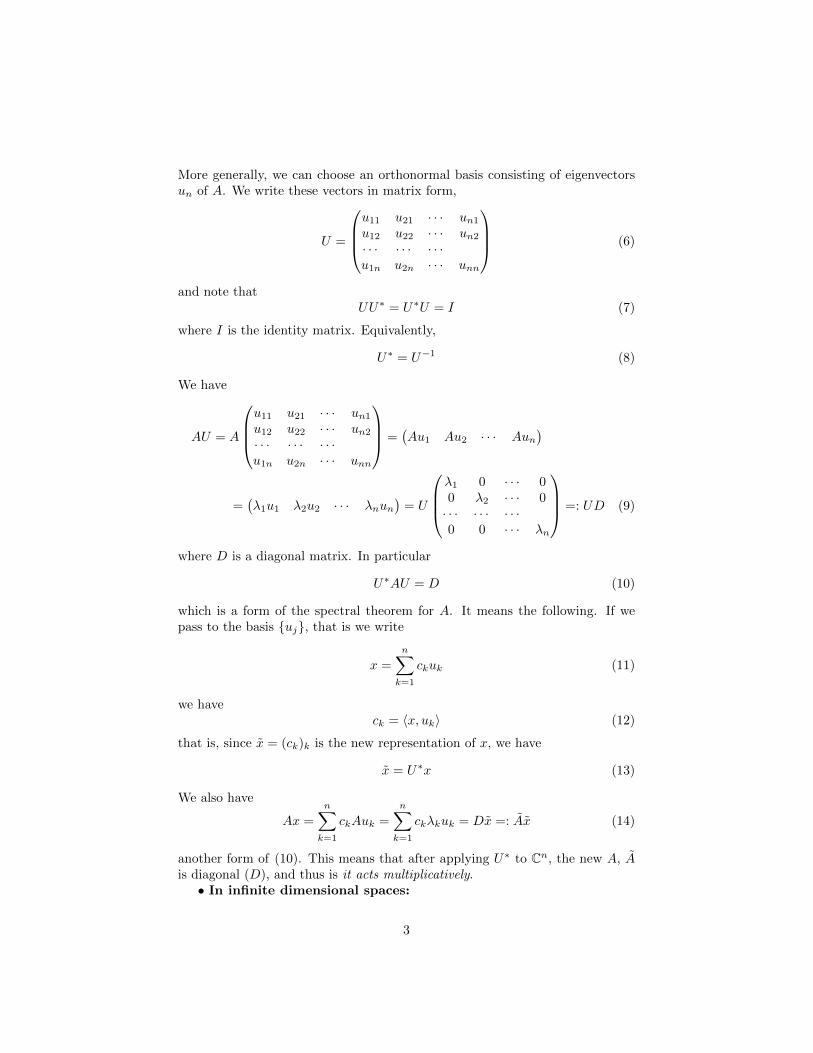
More generally, we can choose an orthonormal basis consisting of eigenvectorsun of A. We write these vectors in matrix form,

U =

u11 u21 · · · un1

u12 u22 · · · un2

· · · · · · · · ·u1n u2n · · · unn

(6)

and note thatUU∗ = U∗U = I (7)

where I is the identity matrix. Equivalently,

U∗ = U−1 (8)

We have

AU = A

u11 u21 · · · un1

u12 u22 · · · un2

· · · · · · · · ·u1n u2n · · · unn

=(Au1 Au2 · · · Aun

)

=(λ1u1 λ2u2 · · · λnun

)= U

λ1 0 · · · 00 λ2 · · · 0· · · · · · · · ·0 0 · · · λn

=: UD (9)

where D is a diagonal matrix. In particular

U∗AU = D (10)

which is a form of the spectral theorem for A. It means the following. If wepass to the basis uj, that is we write

x =

n∑k=1

ckuk (11)

we haveck = 〈x, uk〉 (12)

that is, since x = (ck)k is the new representation of x, we have

x = U∗x (13)

We also have

Ax =

n∑k=1

ckAuk =

n∑k=1

ckλkuk = Dx =: Ax (14)

another form of (10). This means that after applying U∗ to Cn, the new A, Ais diagonal (D), and thus is it acts multiplicatively.• In infinite dimensional spaces:

3

Eq. (1) stays as a definition but the sup may not be attained.

Definition (2) stays.

Property (3) will not be generally true anymore.

(4) will still be valid for bounded operators but generally false for un-bounded ones.

(5) stays.

(14) properly changed, will be the spectral theorem.

Let us first look at L2[0, 1]; here, as we know,

〈f, g〉 =

∫ 1

0

f(s)g(s)ds

We can check that X, defined by

(Xf)(x) = xf(x)

is symmetric. It is also bounded, with norm 6 1 since∫ 1

0

s2|f(s)|2ds 6∫ 1

0

|f(s)|2ds (15)

The norm is exactly 1, as it can be seen by choosing f to be the characteristicfunction of [1 − ε, ε] and taking ε → 0. Note that unlike the finite dimensionalcase, the sup is not attained: there is no f s.t. ‖xf‖ = 1.

What is the spectrum of X? We have to see for which λ X − λ is notinvertible, that is the equation

(x− λ)f = g (16)

does not have L2 solutions for all g. This is clearly the case iff λ ∈ [0, 1].But we note that σ(X) has no eigenvalues! Indeed,

(x− λ)f = 0⇒ f = 0∀x 6= λ⇒ f = 0 a.e,⇒ f = 0 in the sense of L2 (17)

Finally, let us look at X on L2(R). The operator stays symmetric, wherever de-fined. Note that now X is unbounded, since, with χ the characteristic function,

xχ[n,n+1] > nχ[n,n+1] (18)

and thus ‖X‖ > n for any n. By Hellinger-Toeplitz, proved in the sequel seep. 9, X cannot be everywhere defined. Specifically, f = (|x| + 1)−1 ∈ L2(R)whereas |x|(|x|+ 1)−1 → 1 as x→ ±∞, and thus Xf is not in L2. What is thedomain of definition of X (domain of X in short)? It consists of all f so that

f ∈ L2 and xf ∈ L2 (19)

4

It is easy to check that (19) is equivalent to

f ∈ L2(R+, (|x|+ 1)dx) := f : (|x|+ 1)f ∈ L2(R) (20)

This is not a closed subspace of L2. In fact, it is a dense set in L2 since C∞0is contained in the domain of X and it is dense in L2. X is said to be denselydefined.

3 Bounded and unbounded operators

1. Let X, Y be Banach spaces and D ⊂ X a linear space, not necessarilyclosed.

2. A linear operator is a linear map T : D → Y .

3. D is the domain of T , sometimes written dom (T ), or D (T ).

4. The range of T , ran (T ), is simply T (D).

5. The graph of T is

G(T ) = (x, Tx)|x ∈ D (T )The graph will play an important role, especially in the theory of un-bounded operators.

6. The kernel of T is

ker (T ) = x ∈ D (T ) : Tx = 0

3.1 Operations

1. If X,Y are Banach spaces, then T is continuous iff ‖T‖ <∞. Indeed, inone direction we have ‖T (x− y)‖ 6 ‖T‖‖x− y‖, and finite norm impliescontinuity. It is easy to check that if ‖T‖ = ∞ then there is a sequencexn → 0 s.t. ‖Txn‖ 6→ 0.

2. aT1 + bT2 is defined on D (T1) ∩ D (T2).

3. if T1 : D (T1) ⊂ X → Y and T2 : D (T2) ⊂ Y → Z then T2T1 : x ∈D (T1) : T1(x) ∈ D (T2).In particular, if D (T ) and ran(T ) are both in the space X, then, in-ductively, D (Tn) = x ∈ D (Tn−1) : T (x) ∈ D (T ). The domain maybecome trivial.

4. Inverse. The inverse is defined iff ker (T ) = 0. This condition impliesT is bijective. Then T−1 : ran (T )→ D (T ) is defined as the usual functioninverse, and is clearly linear. ∂ is not invertible on C∞[0, 1]: ker ∂ = C.How about ∂ on C∞0 ((0, 1)) (the set of C∞ functions with compact supportcontained in (0, 1))?

5

5. Spectrum . Let X be a Banach space. The resolvent set of an operatorT : D → X is defined as

ρ(T ) = λ ∈ C :

(T − λ) is one-to-one from D to X and (T − λ)−1 : X → D is bounded

See also Corollary 39 below.

The spectrum of T , σ(T ) = C \ ρ(T ). There are various reasons for(T − λ)−1 not to exist: (T − λ) might not be injective, (T − λ)−1 mightbe unbounded, or not densely defined. These possibilities correspond todifferent types of spectra that will be discussed later.

6. Closable operators. It is natural to extend functions by continuity,when possible. If xn → x and Txn → y we want to see whether we candefine Tx = y. Clearly, we must have

xn → 0 and Txn → y ⇒ y = 0, (21)

since T (0) = 0 = y. Conversely, (21) implies the extension Tx := ywhenever xn → x and Txn → y is consistent and defines a linear operator.

An operator satisfying (21) is called closable. This condition is the sameas requiring

G(T ) is the graph of an operator (22)

where the closure is taken in X ⊕ Y . Indeed, if (xn, Txn)→ (x, y), then,by the definition of the graph of an operator, Tx = y, and in particularxn → 0 implies Txn → 0. An operator is closed if its graph is closed. Itwill turn out that symmetric operators are closable.

7. Clearly, bounded operators are closable, since they are continuous.

8. Common operators are “usually” closable. E.g., ∂ defined on a subset of

continuously differentiable functions is closable. Assume fnL2

→ 0 (in the

sense of L2) and f ′nL2

→ g. Since f ′n ∈ C1 we have

fn(x) − fn(0) =

∫ x

0

f ′n(s)ds = 〈f ′n,χ[0,x]〉 → 〈g,χ[0,x]〉 =

∫ x

0

g(s)ds

(23)

Thus

(∀x) limn→∞

(fn(x)− fn(0)) = 0 =

∫ x

0

g(s)ds (24)

implying g = 0.

6. As an example of non-closable operator, consider, say L2[0, 1] (or anyseparable Hilbert space) with an orthonormal basis en. Define Nen =

6

ne1, extended by linearity, whenever it makes sense (it is an unboundedoperator). Then xn = en/n → 0, while Nxn = e1 6= 0. Thus N is notclosable.

Every infinite-dimensional normed space admits a nonclosable linear op-erator. The proof requires the axiom of choice and so it is in generalnon-constructive.

The closure through the graph of T is called the canonical closure of T .

Note: if D (T ) = X and T is closed, then T is continuous, and conversely(see p.9, 5).

7. Non-closable operators have as spectrum the whole of C. Indeed, if T isnot closable, you can check that neither is T − λ, λ ∈ C. We then haveto show that T is not invertible. If xn → 0 and Txn = yn → y 6= 0 thenT−1Txn = T−1yn → T−1y but T−1Txn = xn → 0, thus T−1y = 0 ∈D(T ) since D(T ) has to be a linear space and T (0) = 0, since T is linear,contradiction.

3.1.1 Adjoints of unbounded operators.

1. Let H,K be Hilbert spaces (we will most often be interested in the caseH = K), with scalar products 〈, 〉H and 〈, 〉K.

2. T : D(T ) ⊂ H → K is densely defined if D(T ) = H.

3. Assume T is densely defined.

4. The adjoint of T is defined as follows. We look for those y for which

∃ v = v(y) ∈ H s.t.∀ x ∈ D(T ), 〈y, Tx〉K = 〈v, x〉H (25)

Since D(T ) is dense, such a v = v(y), if it exists, is unique.

5. We define D(T ∗) to be the set of y for which v(x) as in (132) exists, anddefine T ∗(y) = v. Note that Tx ∈ K, y ∈ K, T ∗y ∈ H.

6. Unbounded operators are called self-adjoint if they coincide with theiradjoint, meaning also that they have the same domain. We will return tothis.

In L2[0, 1] consider the “extrapolation” operator E densely defined on poly-Exercise*nomials by E(P )(x) = P (x + 1). Is E bounded? Is it injective? Is it closable?What is the domain of its adjoint? Calculate the spectrum σ(E) from the defi-nition of σ. The solution is given in 1, 31.

7

3.1.2 Absolutely continuous functions

Two (obviously equivalent) definitions of the absolutely continuous functions on[a, b], AC[a, b] are: (I) There exists an L1 function s.t. f(x) = f(a) +

∫ xag(s)ds

for all x ∈ [a, b]; (II) f is differentiable a.e. on (a, b), f ′ ∈ L1 and f(x) =f(a) +

∫ xaf ′(s)ds for all x ∈ [a, b].

Consider the operator T = i ddx defined onExercise*

H20 (R+) := f ∈ L2(R+) : f ′ ∈ L2(R+); f(0) = 0

Is T symmetric (meaning: 〈f, Tg〉 = 〈Tf, g〉) for all f, g ∈ D(T ))? What isσ(T )? Can you find a symmetric operator having C as spectrum?

3.2 A brief review of bounded operators

1. L(X,Y ) denotes the space of bounded linear operators from X to Y . Wewrite L(X) for L(X,X).

2. The space L(X,Y ) of bounded operators from X to Y is a Banach spacetoo, with the norm T → ‖T‖.

3. We see that T ∈ L(X,Y ) takes bounded sets in X into bounded sets inY .

4. We have the following topologies on L(X,Y ) in increasing order of weak-ness:

(a) The uniform operator topology or norm topology is the one givenby ‖T‖ = sup‖u‖=1 ‖Tu‖. Under this norm, L(X,Y ) is a Banachspace.

(b) The strong operator topology is the one defined by the conver-gence condition Tn → T ∈ L(X,Y ) iff Tnx → Tx for all x ∈ X.We note that if Tnx is Cauchy for every x then, in this topology,Tn is convergent to a T ∈ L(X,Y ). Indeed, it follows that Tnx isconvergent for every x. Now note that ‖Tnx‖ 6 C(x) for every xbecause of convergence. Then, ‖Tn‖ 6 C for some C by the uni-form boundedness principle. But ‖Tx‖ = ‖(T − Tn0 + Tn0)x‖ 6‖(T − Tn0

)x‖+ C‖x‖ → C‖x‖ as n→∞ thus ‖T‖ 6 C.

We write T = s− limTn in the case of strong convergence.

Note also that the strong operator topology is a pointwise convergencetopology while the uniform operator topology is the “L∞” versionof it.

(c) The weak operator topology is the one defined by Tn → T if`(Tn(x)) → `(Tx) for all linear functionals on X, i.e. ∀` ∈ X∗. Inthe Hilbert case, X = Y = H, this is the same as requiring that〈Tnx, y〉 → 〈Tx, y〉 ∀x, y that is the “matrix elements” of T converge.It can be shown that if 〈Tnx, y〉 converges ∀x, y then there is a T sothat Tn→w T .

8

5. Reminder: The Riesz Lemma states that if ϕ ∈ H∗, then there is a uniqueyϕ ∈ H so that ϕx = 〈x, yϕ〉 for all x.

6. Adjoints. Let first X = Y = H be separable Hilbert spaces and letT ∈ L(H). Let’s look at 〈Tx, y〉 as a linear functional `T (x). It is clearlybounded, since by Cauchy-Schwarz we have

|〈Tx, y〉| 6 (‖y‖‖T‖)‖x‖ (26)

Thus 〈Tx, y〉 = 〈x, yT 〉 for all x. Define T ∗ by 〈x, T ∗y〉 = 〈x, yT 〉. Using(26) we get

|〈x, T ∗y〉| 6 ‖y‖‖T‖‖x‖ (27)

Furthermore

‖T ∗x‖2 = |〈T ∗x, T ∗x〉| 6 ‖T ∗x‖‖T‖‖x‖

by definition , and thus ‖T ∗‖ 6 ‖T‖. Since (T ∗)∗ = T we have ‖T‖ =‖T ∗‖.

7. In a general Banach space, we mimic the definition above, and writeT ′(`)(x) =: `(T (x)). It is still true that ‖T‖ = ‖T ′‖, see [5]. In Hilbertspaces T ∗ is called the adjoint; in Banach spaces it is also sometimes calledtranspose.

1. Uniform boundedness theorem. If Tjj∈N ⊂ L(X,Y ) and ‖Tjx‖ <C(x) <∞ for any x, then for some C ∈ R, ‖Tj‖ < C ∀ j.

2. In the following, X and Y are Banach spaces and T is a linear operator.

3. Open mapping theorem. Assume T : X → Y is onto. Then A ⊂ Xopen implies T (A) ⊂ Y open.

4. Inverse mapping theorem. If T : X → Y is one to one, then T−1 iscontinuous.

Proof. T is open so (T−1)−1 = T takes open sets into open sets.

5. Closed graph theorem T ∈ L(X,Y ) (note: T is defined everywhere) isbounded iff G(T )) is closed.

Proof. It is easy to see that T bounded implies G(T ) closed.

Conversely, we first show that Z = G(T ) ⊂ X ⊕ Y is a Banach space, inthe norm

‖(x, Tx)‖Z = ‖x‖X + ‖Tx‖YIt is easy to check that this is a norm, and that (xn, Txn)n∈N is Cauchy iffxn is Cauchy and Txn is Cauchy. Since X,Y are already Banach spaces,then xn → x for some x and Txn → y = Tx. But then, by the definitionof the norm, (xn, Txn) → (x, Tx), and Z is complete, under this norm,thus it is a Banach space.

9

Next, consider the projections P1 : z = (x, Tx) → x and P2 : z =(x, Tx) → Tx. Since both ‖x‖ and ‖Tx‖ are bounded above by ‖z‖,then P1 and P2 are continuous.

Furthermore, P1 is one-to one between Z and X (for any x there is aunique Tx, thus a unique (x, Tx), and (x, Tx) : x ∈ X = G(T ), bydefinition. By the open mapping theorem, thus P−1

1 is continuous. ButTx = P2P

−11 x and T is also continuous.

6. Hellinger-Toeplitz theorem. Assume T : H → H, where H is a Hilbertspace. That is, T is everywhere defined. Furthermore, assume T is sym-metric, i.e. 〈x, Tx′〉 = 〈Tx, x′〉 for all x, x′. Then T is bounded.

Proof. We show that G(T ) is closed. Assume xn → x and Txn → y. Toshow that the graph is closed we only need to prove that Tx = y. Let x′

be arbitrary. Then limn→∞〈xn, Tx′〉 = 〈x, Tx′〉 = 〈Tx, x′〉 by symmetryof T . Also, limn→∞〈xn, Tx′〉 = limn→∞〈Txn, x′〉 = 〈y, x′〉 by symmetry(and by assumption). Thus, 〈Tx, x′〉 = 〈y, x′〉 ∀x′ ∈ H and the graph isclosed.

7. Consequence: The differentiation operator i∂, say, with domain is C∞0(and many other unbounded symmetric operators in applications), whichare symmetric on certain domains cannot be extended to the whole space.General L2 functions are fundamentally nondifferentiable.

Unbounded symmetric operators come with a nontrivial domain D (T ) (X, and addition, composition etc are to be done carefully.

Proposition 2. If H is a Hilbert space, and S, T are in L(H), then

1. T ∗∗ = (T ∗)∗ = T

2. ‖T‖ = ‖T ∗‖

3. (αS + βT )∗ = αS∗ + βT ∗

4. (T ∗)−1 = (T−1)∗ for all invertible T in L(H).

5. ‖T‖2 = ‖T ∗T‖Proof. 1. (∀f, g), 〈f, T ∗∗g〉 = 〈T ∗f, g〉 = 〈f, Tg〉

2. ‖Tx‖2 = 〈Tx, Tx〉 = 〈T ∗Tx, x〉 6 ‖T ∗T‖‖x‖ 6 ‖T ∗‖‖T‖ and thus ‖T‖ 6‖T ∗‖ and vice-versa.

3. A calculation.

4. T ∗(T−1)∗ = (T−1T )∗ = I.

5. In one direction we have ‖T ∗T‖ 6 ‖T ∗‖‖T‖ = ‖T‖2. In the oppositedirection, with u unit vectors, we have

‖T‖2 = supu‖Tu‖2 = sup

u〈Tu, Tu〉 = sup

u〈T ∗Tu, u〉 6 ‖T ∗T‖

10

Corollary 3. The algebra generated by T, T ∗ is a C∗-algebra.

Definition 4. If T ∈ L(H), then the kernel of T , ker T is the closed subspacex ∈ H : Tx = 0. The range of T , ran T is the subspace Tx : x ∈ H.

Note that, since T is continuous, kerT is closed.

Proposition 5. If T ∈ L(H), then ker T = (ranT ∗)⊥ and ker T ∗ = (ranT )⊥

Proof. By Proposition 2 it suffices to show the first part. Note that x ∈ kerTimplies (∀y)〈Tx, y〉 = 0 = 〈x, T ∗y〉. In the opposite direction the proof issimilar.

Definition 6. An operator T is bounded below if ∃ε > 0 s.t. (∀x ∈ H), ‖Tx‖ >ε‖x‖.

Proposition 7. If T ∈ L(H) then T is invertible iff T is bounded below andhas dense range.

Proof. First, if T is invertible, then ‖f‖ = ‖T−1Tf‖ 6 ‖T−1‖‖Tf‖ 6 ‖T−1‖‖Tf‖implying ‖Tf‖ > ‖T−1‖−1‖f‖, so T bounded below. The range of T must beH, otherwise T would not be invertible.

Conversely, first note that the bound below implies injectivity: indeed, if‖T (x− y)‖ > ε‖(x− y)‖, then clearly x− y 6= 0⇒ Tx 6= Ty. We need to showthat ranT = H. Let now y ∈ H and yn → y ∈ H and let’s look at T−1yn = xn.Since ‖yn − ym‖ = ‖T (xn − xm)‖ > ε‖xn − xm‖, xn is Cauchy, converging tosome x ∈ H. Clearly, by continuity Tx = y. Recalling that Txn = yn it followsthat ranT = H.

Corollary 8. If T ∈ L(H) s.t. T and T ∗ are bounded below, then T is invert-ible.

Proof. We only need to show that ranT is dense. But the closure of a spaceS is (S⊥)⊥ while (ranT )⊥ = kerT ∗ = 0 (since T ∗ is bounded below). Since0⊥ = H the proof is complete.

Definition 9. Let T ∈ L(H). Then,

1. T is normal if T ∗T = TT ∗.

2. T is self-adjoint, or Hermitian if T = T ∗.

3. T is positive if (∀f ∈ H), 〈Tf, f〉 > 0.

4. U is unitary if UU∗ = U∗U = I.

The setW (T ) := 〈Tu, u〉 : u ∈ H, ‖u‖ = 1 (28)

is called the numerical range of T .

Proposition 10. T is self-adjoint iff W (T ) ⊂ R. In particular, this is the caseif T is positive.

11

Proof. If T is self-adjoint, then

〈Tu, u〉 s-adj.= 〈u, Tu〉; 〈Tu, u〉 def.= 〈u, Tu〉 ⇒ 〈u, Tu〉 ∈ R

Conversely, iu 〈Tu, u〉 ∈ R, then

〈Tu, u〉 = 〈Tu, u〉 = 〈u, Tu〉 ⇒ 〈Tf, f〉 = 〈f, Tf〉∀f ∈ H

and by the polarization identity we have 〈Tf, g〉 = 〈f, Tg〉 for all f, g ∈ H.

What is the adjoint of P defined by P(f)(x) =∫ x

0f? Show that P is not aExercise

normal operator without calculating PP∗ and P∗P.What is the spectrum of PP∗ (where P is as in the previous exercise)?Exercise

Proposition 11. If T ∈ L(H), then T ∗T and TT ∗ are positive.

Proof.〈TT ∗f〉 = 〈T ∗f, T ∗f〉 = ‖T ∗f‖2

Proposition 12. If T is self-adjoint on H then σ(T ) ⊂ R.

Proof. With Γ the Gelfand transform, σ(T ) = ran Γ(T ) = ran Γ(T ∗) = ran Γ(T ) ⊂R.

Direct proof. Since T = T ∗ we only have to show that for λ 6∈ R, T + λ andT + λ are bounded below. If λ = a+ ib we can take Q1 = T − a, note that Q1

is also self-adjoint and show that Q + ib,Q− ib are bounded below. Finally, ifb 6= 0 by taking Q = Q1/b (also self-adjoint) it is enough to show that Q± i arebounded below.

Now

‖(Q± i)u‖2 = 〈(Q± i)u, (Q± i)u〉 = 〈Qu,Qu〉+ 〈u, u〉 > 1

Corollary 13. If T is a positive operator then σ(T ) ⊂ [0,∞).

Proof. By Proposition 10, T is self-adjoint, and by Proposition 11 σ(T ) ⊂ R.Let λ = −a, a > 0. We want to show that T + a is bounded below:

‖T +a‖ = 〈(T +a)u, (T +a)u〉 = 〈Tu, Tu〉+2〈Tu, u〉+a2〈u, u〉 > a2〈u, u〉 (29)

and thus T + a = (T + a)∗ is invertible.

12

4 Spectral theorem for bounded normal opera-tors (continuous functional calculus)

Theorem 2. (1) If N is a normal operator in a Hilbert space H, then theC∗-algebra CN generated by N is commutative. The maximal ideal space Mof CN is homeomorphic to σ(N) and the Gelfand transform Γ is a ∗ isometricisomorphism of C onto C(σ(N)).

Note 1. For normal operators, since M is homeomorphic to σ(N), by abuse ofnotation write that ran ΓN = C(σ(N)).

Proof. Since N and N∗ commute, the polynomials in N,N∗ form a commutativeself-adjoint subalgebra C1 of L(H) thus contained in the C∗-algebra generatedby N . The closure of C1 is clearly a C∗-algebra containing N , thus it equalsCN . In particular, CN is commutative.

Now we define the homeomorphism between C and C(σ(N)) as follows: anelement of M can be identified with a multiplicative functional ϕ. We want tomap ϕ to a unique point in σ(N). The natural way is to take ϕ(N). That is,ψ(ϕ) = Γ(N)(ϕ) =: ΓNϕ. Note that ran ΓN = σ(N) and thus ψ is onto. Weneed to check injectivity.

Assume ψ(ϕ1) = ψ(ϕ2). It means that

ΓNϕ1 = ΓNϕ2 ⇔ ϕ1(N) = ϕ2(N) (30)

and also

ΓN∗ϕ1 = ΓNϕ1 = ΓNϕ2 = ΓN∗ϕ2 ⇔ ϕ1(N∗) = ϕ2(N∗) (31)

Thus, by linearity and multiplicativity, ψϕ1 and ψϕ2 take the same value on allpolynomials in N,N∗ and by its continuity, on all of CN .

It remains to show bicontinuity, which simply follows from the map beingone-to-one between Hausdorff spaces and from continuity of ψ which is easilychecked:

limβ∈B

ψ(ϕβ) = limβ∈B

ΓNϕβ = limβ∈B

ϕβ(N) = ϕ(N) (32)

by the continuity of ϕ.

5 Functional calculus

We see that, for a normal operator T , Γ is an isomorphism between CT and aspace of continuous functions on a domain in σ(T ) ⊂ C. If F is in C(σ(T ))we can simply define F (T ) := Γ−1(F ). We have already indirectly used thespectral theorem in Proposition 12.

(1)As we will see from the proof, the assumption that we are dealing with the algebragenerated by an operator, rather than the one generated by some abstract element in anabstract C∗-algebra is not needed, so this theorem is more general.

13

It is easy to check that any polynomial P in T , which can be defined directlyin CT coincides with Γ−1(P ). In fact polynomials can be defined in any CTregardless of whether T is normal or not. But in both cases, it is very desirableto extend the functional calculus beyond these types of functions, as we’ll see ina moment. For normal operators this is because we need to define projectionsand other L∞ functions while C(M) is already closed in ‖ ‖∞; we will thereforeneed to weaken the topology.

Before that we will use this calculus to derive some fundamental propertiesof normal operators.

Proposition 14. (i) Assume T is normal in L(H). Then, T is positive iffσ(T ) ∈ [0,∞). (ii) T is self-adjoint iff σ(T ) ⊂ R.

Proof. (ii) was proved in Proposition 12. For (i) recall from Theorem 2 thatΓ is an isomorphism. We also know (this is general) σ(T ) = ran ΓT . Sinceσ(T ) ⊂ [0,∞) it follows that ΓT > 0. Then, there exist (many (2)) F ∈C(σ(T )) s.t. Γ(T ) = |F |2 = FF ⇒ T = Γ−1(F )(Γ−1(F ))∗ which we alreadyproved is positive. If T is positive the result follows from Proposition 10 andCorollary 13.

Since the condition σ(f) ∈ [0,∞) makes sense in an abstract C∗-algebra, itallows us to define a positive element of a C∗-algebra as a normal element withthe property σ(f) ∈ [0,∞).

5.1 Projections

These are very important tools in developing the spectral theorem.

Definition 15. A self-adjoint operator P is a projection if P 2 = P .

Note that, in particular, projectors are positive.

Proposition 16. Projections are into a one-to-one correspondence with closedsubspaces of H: PH = M is always a closed subspace of H, and if M is a closedsubspace and we decompose x = xM + x⊥ where xM ∈ M and x⊥ ⊥ M , thenx 7→ Px = xM is a projection.

Proof. Note that P⊥ = (1−P ) is also a projector, since 1−P is self-adjoint, and(1− P )2 = 1− 2P + P = 1− P . Evidently, we can write x = Px+ (1− P )x =x1 + x2, and x1 ⊥ x2 since 〈x1, x2〉 = 〈Px, (I − P )x〉 = 〈x, (Px − Px)〉 = 0.Note also that x ∈ ranPx is equivalent to x = Px, or x ∈ ker (P − I) which isclosed. Thus ranP is closed and so is ran (1− P ). Thus, ranP and ran (1− P )are mutually orthogonal closed subspaces of H.

If now M is a closed subspace of H, then we can perform the orthogonaldecomposition x = xM+x⊥. Note that x 7→ xM is a linear operator PM of normless than one and P 2

M = PM . We have 〈PMf, f〉 = 〈fM , fM + f⊥〉 = ‖fM‖2 > 0and thus P is self-adjoint.

(2)e.g.√

Γ(T ).

14

Proposition 17. Let M1, ...,Mn be closed subspaces of H, and let P1, ..., Pnbe the associated projection operators. Then PiPj = 0 iff Mi ⊥ Mn and P1 +...+ Pn = I iff the span of M1, ...Mn = H.

Proof. Assume PiPj = 0 if i 6= j. x ∈ ranPj iff x = Pjx and also, by definition,if x ∈ Mj . But then Px ⊥ Mi and thus PiPjx = 0. If Mj span H, then bydefinition x = x1 + ...+xn where xk ∈Mk and the xk are mutually orthogonal.This also means, by the definition of Pj that (∀x), x = P1x+ ...+Pnx and thusP1 + ...+ Pn = I. We leave the converse as an exercise.

Note now that for a finite-dimensional operator A with eigenvalues λ1, ..., λn,the polynomial

∏j1(A−λi) is a projector onto the span of eigenvectors and gen-

eralized eigenvectors corresponding to λj+1, ..., λn. In an infinite-dimensionalcontext, a corresponding infinite product may make no sense, but the inverseimage through Γ of the characteristic function of [a, b] ⊂ σ(A) should be a pro-jector, since it is real valued and equal to its square. Note however that, unlessσ(A) is disconnected or the topology is otherwise cooperating, characteristicfunctions are not continuous and Γ−1 of a characteristic function is not defined.This is one reason we need to extend functional calculus.

5.2 Square roots

The proof of Proposition 14 suggests that we can define the square root of apositive operator, and a canonical one if we insist the square root be positive.

Proposition 18. If P is a positive operator in L(H), then there exists a uniquepositive operator Q s.t. Q2 = P . Moreover, Q commutes with any operatorcommuting with P .

Proof. As in the proof of Proposition 14 the fact that, if f is a continuousnonnegative function so is

√f allows us to define Q =

√P = Γ−1(

√Γ(P )). If

Q1 is any positive operator s.t. Q21 = P , then Q1 commutes with P as seen

by writing Q31 = (Q2

1)Q1 = Q1(Q1)2. Furthermore, a unique positive squareroot of P exists in the commutative algebra generated by Q which contains (infact equals) the C∗-algebra generated by P ; this is seen by looking through theisomorphism Γ at an equation of the form F 2 = G2 where F and G are positive:they must clearly coincide. The last part is obvious since the C∗-algebra’sgenerated by Q and P coincide.

Corollary 19. Let T ∈ L(H). Then T is positive iff there is an S ∈ L(H) s.t.T = S∗S.

Proof. If T is positive, we can simply take S =√T . If T = S∗S this follows

from Proposition 11.

Lemma 20. Let T ∈ L(H) and B the Banach algebra generated by T . Thenthe space of maximal ideals of T is homeomorphic to σ(T ) and Γ(B) is containedin the closure in the sup norm of polynomials on σ(T ).

15

Proof. Let ϕ be a multiplicative functional. Then λ = ϕ(T ) ∈ ran Γ = σ(T ).As in the proof of the Gelfand-Naimark theorem let ψ(ϕ) = ΓT (ϕ) = ϕ(T ) = λ.Once more, since ran ΓT = σ(T ), ψ P (x) =

∑n0 cnx

n is a polynomial, thenΓP (T )(ϕ) = ϕ(P (T )) = P (λ). If ψ(ϕ1) = ψ(ϕ2), then, by definition ΓT (ϕ)1 =ΓT (ϕ)2, thus ϕ1(T ) = ϕ2(T ) and ϕ1(P (T )) = ϕ2(P (T )) for any polynomial.Since by definition P (T ) are dense in B, by continuity, ϕ1 = ϕ2 on B. Continuityof ψ is shown as in the Gelfand-Naimark theorem. Now, ‖Γ(X)‖∞ 6 ‖X‖B andthus Γ maps B onto a subspace of the closure of polynomials on σ(T ) in the supnorm.

5.3 Example: the right shift

Example 21. 1. The right shift S+ on l2(N) defined by (x1, x2, x3, ...) →(0, x1, x2, ...) is clearly an isometry but (1, 0, ...) is orthogonal to ranS,and thus S is not invertible (note that S− := (x1, x2, x3, ...) 7→ (x2, x3, ...)is a left inverse, S−S+ = I but S+S− is the projection to the subspaceorthogonal on e1,H⊥1 .

2. It is easy to check that S∗+ = S− and, by the above, S+ is thus not anormal operator: S∗+S+ = I while S+S

∗+ is the projection on H⊥1 .

3. Note also that the Banach algebra (not the C∗-algebra!) B generated byS+ is commutative. The spectrum of S+ is contained in D since ‖S+‖ = 1.The spectrum of S+ is D (indeed, solving S+s − λs = u is equivalent tosolving, coefficient by coefficient, the equation zF − λF = U , in a spaceof analytic functions of the form F =

∑∞n=0 skz

k with∑∞n=0 |sk|2 < ∞.

This implies that F is analytic in D. If λ ∈ D it is clear that, with sayu = (1, 0, 0...) there is no analytic solution in D. Since the spectrum isclosed, the spectrum is thus D.

4. By Lemma 20 B is contained in the closure of polynomials in the sup normon D, and this clearly consists of functions analytic in D and continuouson D.

5. Associating to s ∈ l2(N) an analytic function in the open unit disk,∑n snz

n we see that S+ becomes multiplication by z.

6. The maximal ideal space is the closed unit disk, and the shift is perhapsbetter seen through the Gelfand transform: given f , analytic with abso-lutely convergent Taylor series the right shift corresponds to f(z) 7→ zf(z)and this has an inverse, f → f/z which is defined on a proper subspaceof analytic functions. Recall (and it is obvious) that Γ is not onto from Bto C(M). The left shift is [f(z)− f(0)]/z, which does not commute withmultiplication by z, as expected.

7. By Lemma 20 Γ(B) is contained in the closure in the sup norm of poly-nomials on D which are the analytic functions on D continuous on D, aspace much smaller than C(M) = C(D).

16

6 Partial isometries

Definition 22. An operator V on H is a partial isometry if for any f ⊥ kerVwe have ‖V f‖ = ‖f‖. If, in addition ker(V )= 0, then V is an isometry. Theinitial space of a partial isometry is (kerV )⊥.

Note that in Cn any isometry is a unitary operator. In infinite dimensionalspaces this not true in general (look, e.g., at S−). The existence of a partialisometry between two closed subspaces S1 and S2 only depends on whether thesubspaces have the same dimension (in terms of the cardinality of the basis).

Proposition 23. Assume S1, S2, subsets of H, have the same dimension. Thenthere is a partial isometry V : S1 with range S2.

Proof. Let eαα∈A be a basis in S1 and fαα∈A be a basis in S2. For x ∈ Hdecompose x = x⊥ +

∑α∈A xαeα where x⊥ is orthogonal to S1. Define now

V x :=∑α∈A

xαfα (33)

6.1 Characterization of partial isometries

Lemma 24. For any operator A, kerA = kerA∗A. In one direction it’s clear:Af = 0⇒ A∗A = 0. Conversely, if A∗A = 0, then

〈A∗Af, f〉 = 〈Af,Af〉 = ‖Af‖2 = 0⇒ Af = 0 (34)

Lemma 25. If P is a positive operator, then 〈Pf, f〉 = 0⇒ Pf = 0.(3)

Proof. We write

〈Pf, f〉 = 〈(P 1/2)2f, f〉 = 〈P 1/2f, P 1/2f〉 = 0⇒ P 1/2f = 0⇒ Pf = 0

Proposition 26. Let V be an operator on the Hilbert space H. The followingare equivalent:

1. V is a partial isometry.

2. V ∗ is a partial isometry.

3. V V ∗ is a projection.

4. V ∗V is a projection

(3)Separated from the main proofs at the suggestion of I. Glogic.

17

If moreover V is a partial isometry, then V V ∗ is the projection onto the rangeof V and V ∗V is the projection onto the initial space of V (S1 in Proposition23 above.)

Proof. Assume V is a partial isometry. For any f ∈ H we have

〈(1− V ∗V )f, f〉 = 〈f, f〉 − 〈V ∗V f, f〉 = 〈f, f〉 − 〈V f, V f〉 > 0 (35)

and thus 1 − V ∗V is a positive operator. By definition, if f ⊥ kerV , then‖V f‖ = ‖f‖ which means 〈(1−V ∗V )f, f〉 = 0. By Lemma 25 we have V ∗V f =f . Conversely, assume that V ∗V is a projection and f ⊥ ker (V ∗V ) = kerV byLemma 24; then V ∗V f = f , thus

‖V f‖2 = 〈V f, V f〉 = 〈V ∗V f, f〉 = ‖f‖2

and thus V preserves the norm on ker (V ∗V )⊥ implying that V is a partialisometry and 4 and 1 are equivalent. Similarly, 2 and 3 are equivalent.

Now we show that 3 and 4 are equivalent. We first note that V (V ∗V ) = V .Indeed, if f ∈ kerV = kerV ∗V , then of course V (V ∗V )f = 0 = V f . Iff ⊥ kerV ∗V , then, since V ∗V is a projection, = V V ∗V f = V f = V .

Hence,

(V V ∗)2 = V (V ∗V )V ∗ = V V ∗

The rest is a straightforward verification.

7 Polar decomposition of bounded operators

An analog of the polar representation z = ρeit familiar from complex analysisexists for bounded operators as well.

Note 2. 1. Recall that (T ∗T ) and TT ∗ are positive and thus have squareroots, obviously positive too. As a candidate for ρ, note first that, if Tis a normal operator, one can define |T | simply by Γ−1(|ΓT |). In general,we have two obvious candidates, |T |2 = T ∗T and |T |2 = TT ∗. The rightchoice is T ∗T however, as it preserves the norm of the image:

‖(T ∗T )1/2f‖2 = 〈(T ∗T )1/2f, (T ∗T )1/2f〉 = 〈Tf, Tf〉 = ‖Tf‖2 (36)

(this is of course stronger than ‖T‖ = ‖T ∗‖ = ‖(T ∗T )1/2‖ = ‖(TT ∗)1/2‖).

2. We first note that we can’t expect to have a representation of the formT = |T |U with U unitary since, for instance (see Example 21) S∗+S+ =

I = (S∗+S+)1/2 and thus the equality S+ = (S∗+S+)1/2U as well as S+ =

U(S∗+S+)1/2U are impossible. However S+ itself is an isometry (withnontrivial kernel).

Definition 27. We naturally set |T | := (T ∗T )1/2.

18

Note 3. |T | does not behave like the absolute value of a functions. It is falsethat |A| = |A∗| or |A||B| = |AB|, or even that |A|+ |B| 6 |A|+ |B|.

Theorem 3. Let T ∈ L(H). Then there exist partial isometries s.t.

1. T = V |T |;

2. T = |T |W .

Moreover a polar decomposition of the form T = V1P is the one above ifkerP = kerV1; same with the decomposition T = QV2 if ranW = (kerQ)⊥.

Proof. We have already shown that ‖Tf‖ = ‖|Tf |‖. It is natural to define Von ran |T | by V |T |f = Tf , as this is what we want to achieve. If we extend Vby zero on (ran |T |)⊥ = (ranT )⊥, it is easy to see that V is a partial isometry.

We have, by definition kerV = (ran |T |)⊥ = ker |T |.For uniqueness, assume we have a decomposition T = V1P as above. Since

V1, V∗1 are partial isometries and kerV1 = kerP = (ranP )⊥, we have V ∗1 V1P =

P . It follows that|T |2 = T ∗T = PV ∗1 V1P = P 2 (37)

Uniqueness of the square root implies P = |T | which in turn implies V1 = Von ran |T |. But (ran |T |⊥) = ker |T | = kerP = kerV1, and thus V1 = V on(ran |T |⊥) as well.

Uniqueness of 2 follows from 1 in a straightforward way, going through thesame steps but with T ∗ instead of T , and is left as an exercise.

Another general fact will be useful in the sequel.

Proposition 28. If A ∈ L(H) is bounded below by a and is invertible, then‖A−1‖ 6 a−1.

Proof.

‖A−1‖ = supx

‖A−1x‖‖x‖

= supy

‖y‖‖Ay‖

6 a−1

8 Compact operators

We mention a useful general formula, whose proof is a simple verification. It isthe non-commutative extension of a−1 − b−1 = (b− a)a−1b−1.

Proposition 29 (Second resolvent formula). Assume A and B are invertibleoperators. Then

A−1 −B−1 = A−1(B −A)B−1 (38)

Corollary 30. If B is invertible and ‖(B − A)B−1‖ = ‖I − AB−1‖ < 1, thenA is invertible and

A−1 = B−1(1− (B −A)B−1)−1 (39)

19

Proof. A calculation starting with (38) gives

A−1(1− (B −A)B−1) = B−1 ⇒ A−1 = B−1(1− (B −A)B−1)−1 (40)

This of course is a formal calculation, but is easily transformed into a rigorousproof inverting both sides of (39):

A = (1− (B −A)B−1)B (41)

That this equality holds is an immediate calculation, and now invertibility of Aand formula (40) are obvious.

Operators of the form

(Kf)(x) =

∫ 1

0

K(x, y)f(y)dy (42)

are seen throughout analysis, for instance as solutions of differential equations.Assuming the original problem is not singular, often K is at least continuousfor (x, y) ∈ [0, 1]2. We will look first at this case.

The operator K in (43) with F ∈ C([0, 1]2 is clearly bounded in L∞[0, 1]by M = sup[0,1]2 K(x, y) , and continuous. But Fredholm noticed that there issomething more going on, and of substantial importance. Since K is continuouson [0, 1]2, it is uniformly continuous: for any ε there is a δ s.t. |x−x′|+|y−y′| < δimplies |K(x, y)−K(x′, y′| < ε in [0, 1]2. This implies

|(Kf)(x)− (Kf)(x′)| =∣∣∣∣∫ 1

0

[K(x, y)−K(x′, y)]f(y)dy

∣∣∣∣ 6Mε (43)

Let BR be the ball of radius R in C[0, 1] (43) implies that K(BR) is a set ofequibounded, equicontinuous functions, and thus, by Ascoli-arzela, precompact.That is, K maps a sequence of equibounded functions into a sequence havingconvergent subsequences. Fredholm showed that such operators have especiallygood features, including what we now know as the Fredholm alternative prop-erty. According to [5] p. 215, Fredholm’s work “produced considerable interestamong Hilbert and his school, and led to the abstraction of many notions wenow associate with Hilbert space theory”.

Definition 31. Let X,Y be Banach spaces. An operator K ∈ L(X,Y ) is calledcompact if K maps bounded sets in X into precompact sets in Y .

Equivalently, K is compact if for any sequence (xn)n∈N the sequence (Kxn)n∈Nhas a convergent subsequence.

Integral operators of the type discussed at the beginning of this section aretherefore compact.

Another important class of examples is provided by operators of finite-rank(called degenerate in [4]). These are by definition operators in L(X,Y ) withfinite dimensional range.

20

Proposition 32. Operators of finite rank are compact.

Proof. Writing the elements of KX in terms of a basis, Kx =∑nk=1 xnen,

xn ∈ C and en linearly independent in KX, this is an immediate consequenceof the fact that any bounded sequence in Cn has a convergent subsequence.

An important criterion (that was introduced as a definition of compact op-erators by Hilbert) is the following.

Theorem 4. A compact operator maps weakly convergent sequences into normconvergent ones.

Proof. Assume xnw→x. The uniform boundedness theorem implies that ‖xn‖

are bounded. Denote by ` the elements of X∗ and yn = Kxn. The sequenceyn is also weakly convergent to y = Kx since by the definition of the adjoint(“transposed” in [4]) operator K ′ and its boundedness we have, with

|`yn − `y| = |(K ′`)(xn − x)| (44)

is convergent since (K ′`) is a continuous functional. Suppose to get a contradic-tion that yn did not converge in norm to Kx. Then there would exist an ε > 0sequence ynk

= Kxnks.t. ‖ynk

− y‖ > ε for all k ∈ N. Since K is compact, asubsequence of the ynk

would converge in norm to some y 6= y. But this wouldimply that the subsequence also converges weakly to y, contradiction.

Proposition 33. If X is reflexive, then the converse of Theorem 4 holds, andif B is the unit ball in X, then KB is compact.

For reflexive spaces therefore, Hilbert’s definition coincides with Definition31.

Proof. Because X is reflexive, the unit ball in X is weakly compact (cf. [7]p.251) (because it is homeomorphic to the unit ball in the dual of X∗). Wewant to show KB is compact in norm. Let xnn ∈ B. Thus we can extract aweakly convergent subsequence xnk

. But then, by assumption, Txnkis norm-

convergent.

Theorem 5. Let K ∈ L(X,Y ), where X,Y are Banach spaces. Then

1. The norm limit of a sequence of compact operators is compact.

2. K is compact iff K ′ is compact.

3. If S1, S2 are bounded operators, and K is compact, then SK and KS arecompact (that is, compact operators are an ideal in the space of boundedoperators).

Note 4. In particular the norm limit of finite rank operators is compact.

21

Proof. 1. Let (Kn)n∈N be the compact operator sequence and let xjj∈N bebounded (say, by one) and for each n extract a convergent subsequencexjn and by the diagonal trick we can extract a sub-subsequence xjnk

s.t.Knxjnk

→ yn for any n. We have ‖xn‖ 6 1 and supnKn = M < ∞since (Kn)n∈N is norm-convergent. Then an ε/3 argument shows that ynconverges. Then, in a similar way it follows that Kxjnk

→ y.

2. Assume K is compact. Let (`n)n∈N ∈ X∗ be bounded by 1. Then, `nare clearly equibounded and equicontinuous, as defined on the compactset KB in X. Then, by Ascoli-Arzela there is a subsequence `nk

whichconverges uniformly on KB. Then

supu∈B‖K ′`nk

(u)−K ′`nk′ (u)‖ def= sup

u∈B|`nk

(Ku)− `nk′ (Ku)|

= supy∈KB

|`nk(y)− `nk′ (y)| → 0 (45)

This shows that K ′`nkis norm Cauchy, thus norm convergent.

3. This is straightforward.

From now on we focus on Hilbert spaces, a more frequent setting. In aHilbert space we have a stronger connection between compact operators andfinite rank ones than in Note 4.

Theorem 6. Let H be a separable Hilbert space. Then K : H → H is compactiff K is the norm limit of finite-rank operators.

Proof. In one direction, we proved this already. In the opposite direction, let(en)n∈N be an orthonormal basis in H. We show that K is the limit of FEn

where En is the space generated by e1, ..., en, F = K on En and zero outside.If we let

λn = sup‖Ku‖ : ‖u‖ = 1 and u ∈ E⊥n (46)

clearly, λn is decreasing and positive, thus λn → λ. If we show λ = 0, then theresult is proved. Let un ⊥ ej ∀j 6 n be s.t. ‖Kun‖ > λ/2. The sequence (un)nconverges weakly to zero. But then Kun converges to zero in norm, and thusλ = 0.

We will then study finite rank operator in more detail.

8.1 Finite rank operators

Let F be a finite rank operator: the range of FX = R is isomorphic to Cn forsome n. We choose a basis e1, ..., en in R. We have 〈ei, Fx〉 = 〈fi, x〉 wherefi = F ∗ei. By construction, none of the fi can be zero.

22

Then for all x ∈ H we have

Fx =

n∑i=1

〈Fx, ei〉ei =

n∑i=1

〈x, fi〉ei (47)

We can now apply Gram-Schmidt and make the fi orthogonal, so we can assumethat they are orthogonal to start with. We can write fi = αiui where ui =fi/‖fi‖ form an orthonormal set, and we finally have the normal form of a finiterank operator as

Fx =

n∑i=1

αi〈x, ui〉ei (48)

We will call the space U generated by u1, ..., un the initial space of F .

8.1.1 More about finite-rank operators

1. From (48) we see that F is zero on U⊥. Let FU be the restriction of F toU .

2. The image E = FUU has the same dimension as U , n.

3. Let E′ = U ⊕E and let FE′ = F|E′ . Then clearly F (E′) ⊂ E′ and thus in

the decomposition H = E′ ⊕ E′⊥ we have

F = F|E′ ⊕ 0 dimE′ 6 2n (49)

In this sense, finite rank operators are square matrices on a finite dimen-sional subspace of H and zero outside it.

4. If F is finite-rank then F ∗ is of finite rank since ranF ∗ = (kerF )⊥ =(U⊥)⊥ = U .

5. From (48) we see that zero is always in the spectrum of F if dimH > n.

6. Finite rank operators form an ideal in L(H). Indeed, if F is of finite rankand S ∈ L(H), then clearly ran (FS) ⊆ ranF . In the opposite directionthe proof is essentially the same: (SF )∗ = F ∗S∗ is of finite rank by thefirst part.

7. In analyzing the spectrum of finite rank operators, we note that (49)implies that

λI − F = (λIE′ − F|E′ )⊕ λIE′⊥ dimE′ 6 2n (50)

where IE is the identity on the closed subspace E ⊂ H.

23

8.1.2 The Fredholm alternative, nonanalytic case

Theorem 7 (The Fredholm alternative). (i) If K is a compact operator then(I−K)−1 exists and is bounded iff x = Kx has no nonzero solution, iff (I−K)is bounded below.

(ii) If λ ∈ σ(K) then either λ = 0 or it is an eigenvalue of K of finitemultiplicity. The only possible accumulation point of σ(K) is 0.

Note 5. We could derive this as a corollary of the analytic Fredholm alternativedeveloped in the next section, which relies in fact on similar arguments, but forclarity of the presentation we prefer to prove Theorem 7 first.

Proof. We want to link invertibility of K to the invertibility of a finite rankoperator. In general, an additive approximation, K = F + ε, ‖ε‖ small shouldnot work easily since, generally, the kernel of I −K is bound to differ from thekernel of I−F and the vectors where I−K is not invertible will always dependon ε.

We look for a representation of the form (I − g)(I + ε1) with g of finite rankand ε1 small. This is obtained from K = F + ε for instance by factoring out tothe right I − ε: (4) (factoring out I − F would not have the same drawback asusing additive approximations, it would change the kernel)

(I −K) = (I − F − ε) = (I − F (I − ε)−1)(I − ε) (51)

With obvious notations, we get from (50),

I −K =[(IE′ − gE′)⊕ IE′⊥

](I − ε) (52)

where ε = F −K is an operator of small norm. This can also be obtained fromthe second resolvent formula (41), taking A = I −K and B = I −F . Note thatin (52) (IE′ − gE′) is simply linear operator on the finite-dimensional space E′.

Now assume I−K is bounded below. Then, (IE′−gE′), a finite dimensionaloperator, is bounded below, and thus invertible, implying by (52) is invertible.

In the opposite direction, if I − F is not bounded below, then (52) impliesthat IE′ − gE′ is not bounded below, thus U = ker (IE′ − gE′) 6= 0. Ifui, i = 1, ...,m generate U , then the kernel of I −K is nonempty,

ker (I −K) = U ⊕ 0E′⊥ (53)

(ii) If λ 6= 0, then the equation (λ−K)u = v is equivalent to 1−K ′ = λ−1vwhere K ′ = λ−1K is compact. The fact that only zero is a possible accumulationpoint follows from Corollary 36 below. The rest follows from (i).

Corollary 34. Assume K is compact and ker (I −K) = 0. Then, ran (I −K) = H.

Proof. Indeed, if ran (I −K) 6= H, then I −K is not invertible, and the resultfollows from Theorem 7.

(4)Simplified calculation suggested by C. Xu

24

Corollary 35. If K is compact, then I −K has closed range.

Proof. We have ran (I − ε) = H since it is a continuous bijection, while from(52)

ran (I − g) = ran[(IE′ − gE′)⊕ IE′⊥

]clearly closed.

9 The analytic Fredholm alternative

Setting. Let D be a domain in C, that is an open connected set. Let K :D → L(H) be an analytic operator-valued function s.t. K(z) is compact for allz ∈ D. Then the following alternative holds:

Theorem 8. Either(i) (I −K(z))−1 exists for no z ∈ D, or(ii) (I−K(z))−1 exists in D\S where the set S is discrete (no accumulation

points in the open domain).In case (ii), (I −K(z))−1 is a meromorphic function of z whose residues at

the poles zs (limz→zs(z − zs)ks(I −K(z))−1, ks = order of the pole) are finiterank operators and z ∈ S ⇔ K(z)u = u for some unit vector u.

Proof. We first prove the alternative in some neighborhood of N (z0); from it,one can extended to the whole of D by a standard connectedness argument.Assume that I − K is invertible at some z0. Let N (z0) be small enough s.t.‖K(z) − K(z0)‖ 6 ε∀z ∈ N (z0), choose F s.t. ‖F − K(z0)‖ < ε. Then‖K(z)− F‖ 6 2ε. If ε < 1/2 we write the decomposition (52):

I −K(z) =[(IE′ − gE′(z))⊕ IE′⊥

](I + ˆε(z)) (54)

where ˆε(z) is an operator of small norm if ε is small in (0, 1/2). Since I + ε isanalytic in N (z0), so is g. We then see that

[I −K(z)]−1 = (I + ˆε(z))−1[(IE′ − gE′(z))−1 ⊕ IE′⊥

](55)

Noting that (IE′−gE′(z))−1 is meromorphic by the standard inversion formula,the rest is straightforward.

Note 6. Assuming that det(IE′ − gE′(z)) has a zero of order k at z = zs, thenthe finite rank operator at zs is

F = (I + ˆε(z))−1[ limz→zs

(z − zs)k(IE′ − gE′(z))−1 ⊕ 0] (56)

Corollary 36. The only possible accumulation point in the spectrum of K iszero.

25

Proof. Indeed, other accumulation points would be essential singularities of(K/z − I)−1 which is meromorphic.

Theorem 9 (The Hilbert-Schmidt theorem).

1. Let K be compact and self-adjoint on H (assumed separable and, to avoidtrivialities, infinite dimensional). Then there is an orthonormal basis E =eii∈N for H s.t. Kei = λiei and λn → 0 as n → ∞. In the basis E , Kis therefore diagonal. Each eigenvalue has finite degeneracy.

2. H can be written asH = H0

⊕k

Ek (57)

where K = 0 on H0 (we could have H0 = 0, and then H0 can be omittedfrom the decomposition) and Ek are finite dimensional spaces. On eachEk, H = λkIEk

.

Proof. The spectrum of K cannot be empty, as we know. We also know thatthe spectrum is discrete and real, and it is one of eigenvalues ei, except perhapsfor 0.

1. (*) Assume first that σ(K) = 0. Then, by Theorem 7 and the fact thatK is self-adjoint, ‖K‖ = r(K) = 0. This case is trivial.

(**) We will now look at nonzero eigenvalues. By the usual trick

〈ei,Kek〉 = λk〈ei,Kek〉 = 〈Kei, ek〉 = λi〈ei,Kek〉 (58)

the eigenvectors corresponding to distinct eigenvalues are orthogonal to each-other. Let H1 be the space generated by all ei. We claim that H2 = (H1)⊥ isinvariant under K. Indeed, if f ⊥ ej , then

〈Kf, ej〉 = 〈f,Kej〉 = λj〈f, ej〉 = 0 (59)

Now let K2 be the restriction of K to the Hilbert space H2. Clearly K2 is alsoself-adjoint. K2 cannot have any nonzero eigenvalue inH2 by the construction ofH1, and (*) implies K2 = 0 on H2. The rest of the proof is straightforward.

9.1 Singular value decomposition

A decomposition similar to (48) holds for general compact operators. We could,in principle, pass it to the limit, but there is a shortcut.

Note first that Kx = 0 ⇔ K∗Kx = 0. That Kx = 0 ⇒ K∗Kx = 0is obvious. In the opposite direction, it follows from the polar decompositionK = U |K|.

If K is compact, so is K∗K, and it is also self-adjoint. Let unn∈N be anorthonormal basis of eigenvectors of K∗K corresponding to the eigenvalues µn.Since K∗K > 0, µn > 0. We choose only the u′n corresponding to µn > 0, andlet E be the space generated by the u′n.There must exists at least one nonzeroeigenvalue (otherwise K∗K = 0⇒ K = 0, in which case the result is obvious),

26

so this space is nontrivial. Clearly K∗K = 0 on E⊥, and then K = 0 on E⊥ aswell. Since

〈Kun,Kum〉 = 〈K∗Kun, um〉 = δnmµn (60)

(in particular Kun 6= 0) the Kun also form an orthogonal set, which can be

made orthonormal by taking vn = λnKun, λn = |µ−1/2n |, as seen from (60). If

ψ ∈ H, then we have

Kψ = K = K∑un∈E

〈ψ, un〉un =∑un∈E

λn〈ψ, un〉vn (61)

The λn are called singular values of K. The result is then,

Theorem 10 (Normal form of compact operators). Let K be compact. Thenthere exist an orthonormal sets (not necessarily spanning H) un, vn s.t., with Ethe span of the un, (61) holds for all ψ ∈ H, where the λn are the eigenvaluesof |K|.

(i) If K is compact, is |K| necessarily compact?Exercise(ii) If K2 is compact, is K necessarily compact?

9.1.1 Trace-class and Hilbert-Schmidt operators

We mention another important class of operators, and give some results aboutit without proof (for proofs and other interesting results, see e.g. [5] §VI.6; theproofs are not difficult, but would take some time).

Let e1, e2, ..., en, ... be a basis in H. Let T be a positive operator and definethe trace by trT =

∑n∈N〈en, T en〉. A trace-class operator is one for which

tr |T | <∞. A Hilbert-Schmidt operator is one for which trT ∗T <∞.

Theorem 11. Every trace-class, or Hilbert-Schmidt operator is compact. Acompact K operator is trace-class iff

∑λn <∞ where λn are the singular values

of K and Hilbert-Schmidt if∑λ2n <∞.

Theorem 12. Let (M,µ) be a measure space and H = L2(M,dµ). ThenT ∈ L(H) is Hilbert-Schmidt iff there exists a k ∈ L2(M ×M,dµ⊗ dµ) s.t. forall f ∈ H

(Tf)(x) =

∫k(x, y)f(y)dµ(y) (62)

Moreover

‖T‖2 =

∫|k(x, y)|2dµ(x)dµ(y)

Note 7. The conditions of the theorem above give a criterion of compactnessof T .

27

9.2 Application (O.C.)

Consider the operator K given by (Kf)(x) =∫ x

0f . Its adjoint in L2(0, 1), K∗,

is given by (K∗f)(x) = −∫ x

1f . Indeed,∫ 1

0

f(s)

(∫ s

1

(g(t)dt

)ds =

∫ 1

0

[(∫ s

0

f(u)du

)′ ∫ s

1

g(t)dt

]ds

= −∫ 1

0

g(s)

(∫ s

0

f(u)du

)ds (63)

Check that K, and therefore K∗ are compact. Now, the operator

A =1

2i(K∗ −K) (64)

is then clearly self-adjoint. The spectrum is therefore discrete, and consistsof finite degeneracy eigenvalues accumulating at zero, and the eigenvectors arecomplete in L2(0, 1).

The spectral problem for A is

i

∫ x

0

h(s)ds+ i

∫ x

1

h(s)ds = 2λh (65)

A solution of this equation is clearly C∞ (by a smoothness bootstrapping argu-ment, since h is given in terms of the integral of h). Thus we can differentiate(65) and obtain the equivalent problem

ih = λh′ = 0⇔ h′ = −iλ−1h = 0 with h(0) = −h(1) = −∫ 1

0

h (66)

It is clear that the set of solutions of norm 1 consists exactly of

e(2n+1)ix, n ∈ N ∪ 0 (67)

Therefore, the set e(2n+1)ixn∈Z is an orthonormal basis in L2(0, 1).

Show that e2nπixn∈Z is also an orthonormal basis in L2(0, 1).Exercise

9.2.1 Almost orthogonal bases [4]

A small perturbation of an orthonormal basis is still a basis. This result is dueto Paley and Wiener.

Theorem 13 (Paley-Wiener). Let H be a Hilbert space and enn∈N an or-thonormal basis. Assume vn are vectors s.t.

∞∑n=1

‖en − vn‖2 < M <∞ (68)

and that vn are linearly independent. Then vn also form a basis in H.

28

Proof. (Due to Birkhoff-Rota and Sz. Nagy) We take x ∈ H and write

x =

∞∑k=1

xkek (69)

Let now

B = GN +RN ; GN :=

N∑k=1

〈·, ek〉vk; RN :=

∞∑k=N+1

〈·, ek〉vk; (70)

Let EN be the span of e1, ...eN and Then B − I = GN − IEN+ RN − IE⊥N . If

we show that ‖RN − IE⊥N ‖ → 0 it follows that B − I is a limit of finite rankoperators, thus compact. We have

‖RNx− x‖2 6

( ∞∑n=N+1

|xk|‖ek − vk‖

)2

6∞∑

n=N+1

|xk|2∞∑

n=N+1

‖en − vn‖2 → 0

(71)Then ranB = ran (I − (I −B)) = H unless kerB 6= 0. But if a ∈ kerB, thenthere is a nonzero sequence (an) s.t.

∑akvk = 0, contradiction.

10 Closed operators, examples of unbounded op-erators, spectrum

1. We let X, Y be Banach space. Y ′ is a subset of Y .

2. We recall that bounded operators are closed. Note that T is closed iffT + λI is closed for some/any λ.

3.

Proposition 37. If T : D(T ) ⊂ X → Y ′ ⊂ Y is closed and injective,then T−1 is also closed.

Proof. Indeed, the graph of T and T−1 are the same, modulo switchingthe order. Directly: let yn → y and T−1yn = xn → x. This means thatTxn → y and xn → x, and thus Tx = y which implies y = T−1x.

4.

Proposition 38. If T is closed and T : D(T )→ X is bijective, then T−1

is bounded.

Proof. We see that T−1 is defined everywhere and it is closed, thus bounded.

29

Corollary 39. If T is closed, then σ(T ) = z : (T − z) is not bijective.That is, the possibility (T −z)−1 : Y → dom (T −z) is unbounded is ruledout if T is closed.

(Recall that (T − z)−1 must exist on the whole of Y for T − z to beinvertible.)

As an example of an operator with unbounded left inverse we have (Pf)(x) :=∫ x0f . The left inverse is f 7→ f ′ is unbounded from ranP → L2; however,

ranP = AC ∩ L2 ( L2 (it is only a dense subspace of L2).

5. Show that if T is not closed but bijective between domT and Y , there existExercisesequences xn → x 6= 0 such that Txn → 0. (One of the “pathologies” ofnon-closed, and more generally, non-closable operators.)

6. Recall the definition of the spectrum: 5 on p. 6.

The spectrum of an operator plays a major role in characterizing it andSpectrumworking with it. In “good” cases, there exist unitary transformationsthat essentially transform an operator to a multiplication operator on thespectrum, an infinite dimensional analog of diagonalization of matrices.

For closed operators, there are thus two possibilities: (a) T : D(T ) → Yis not injective. That means that (T − z)x = (T − z)y for some x 6= y,which is equivalent to (T − λ)u = 0, u = x− y 6= 0, or ker (T − λ) 6= 0or, which is the same Tu = λu for some u 6= 0. This u is said to belongto the point spectrum of T . (b) ran (T − λ) 6= Y . There are two caseshere: (1) ran (T − λ) is not dense. This subcase is called the residualspectrum. Such would be the case of a finite rank operator in an infinitedimensional Hilbert space, and (ii) The range is dense but not equal tothe whole target space. Assuming that such a λ is not an eigenvalue, wesay that this part of the spectrum is the continuous spectrum.

7. Operators which are not closable are ill-behaved in many ways. Show thatExercisethe spectrum of such an operator must be the whole of C.

1. Consider the operator X defined by (Xf)(x) = xf(x) on L2([0, 1]). WeExamplesnoted already that σ(X) = [0, 1]. You can show that there is no pointspectrum or residual spectrum for this operator.

2. Consider now the operator X on f ∈ L2(R) | xf ∈ L2(R). Show thatσ(X) = R.

3. Let H and H′ be Hilbert spaces, and let U : H → H′ be unitary. LetExercisesTH → H and consider its image UTU∗. Show that T and UTU∗ have thesame spectrum.

4. Show that −i∂ densely defined on the functions in L2(R) so that f ′ existsand is in L2(R), and that it has as spectrum R. For this, it is useful to

30

use item 3 above and the fact that F , the Fourier transform is unitarybetween L2(R) and L2(R).

5. The spectrum depends very much on the domain of definition. In general,the larger the domain is, the larger the spectrum is. This is easy to seefrom the definition of the inverse.

6. The spectrum of unbounded operators, even closed ones, can be any closedset, including ∅ and C.

7. Let T1 = ∂ be defined on D(T1) = f ∈ C1[0, 1] : f(0) = 0 (5) with valuesin the Banach space C[0, 1] (with the sup norm). (Note also that domTis dense in C[0, 1].) Then the spectrum of T1 is empty.

Indeed, to show that the spectrum is empty, note that by assumption(∂−z)D(T1) ⊂ C[0, 1]. Now, (∂−z)f = g, f(0) = 0 is a linear differentialequation with a unique solution

f(x) = exz∫ x

0

e−zsg(s)ds

We can therefore check that f defined above is an inverse for (∂ − z), bychecking that f ∈ C1[0, 1], and indeed it satisfies the differential equation.Clearly ‖f‖ 6 const(z)‖g‖.

8. What about our general C∗ algebra proof that the spectrum cannot beempty? Also, σ(T1) = ∅ implies that T1 is closed, see the exercise above.

9. Clearly, at least when the spectrum is empty there is no analog of a Gelfandtransform to determine the properties of an operator T from those ofcontinuous functions on the spectrum.

10. At the “opposite extreme”, T0 = ∂ defined on D(T0) = C1[0, 1], a densesubset of the Banach space C[0, 1], has as spectrum C.

Indeed, for any z ∈ C, if f(x; z) = ezx, then T0f − zf = 0.

We note that T0 is closed too, since if fn → 0 then fn−fn(0)→ 0 as well,so we can use 6 and 7 above.

11. The examples above show that a domain has to be specified together withan operator; T0 and T1 have very different behavior.

1. An interesting example is E defined by (Eψ)(x) = ψ(x + 1). This is welldefined and bounded (unitary) on L2(R). The “same” operator can bedefined on the polynomials on [0, 1], an L∞ dense subset of C[0, 1]. Notethat now E is unbounded.

2. E : P [0, 1] → EP [0, 1] is bijective and thus invertible in a function sense.But the inverse is unbounded as seen in a moment.

(5)f(0) = 0 can be replaced by f(a) = 0 for some fixed a ∈ [0, 1].

31

3. It is also not closable. Indeed, since P [0, 1] ⊂ P [0, 2] and P [0, 2] is densein C[0, 2], it is sufficient to take a sequence of polynomials Pn convergingto a continuous nonzero function which vanishes on [0, 1]. Then Pn → 0as restricted to [0, 1] while Pn(x+ 1) converges to a nonzero function, andclosure fails. In fact, Pn can be chosen so that Pn(x+ 1) converges to anyfunction that vanishes at x = 1.

Exercise 1. Show that T2 = ∂ defined on D(T2) = f ∈ C1[0, 1] : f(0) = f(1)has spectrum exactly 2πiZ.

It is also useful to look at the extended spectrum, on C∞ We say that∞ ∈ σ∞(T ) if (T − z)−1 is not analytic in a neighborhood of infinity.

11 Integration and measures on Banach spaces

In the following Ω is a topological space, B is the Borel σ-algebra over Ω, Xis a Banach space, µ is a signed measure on Ω. Integration can be defined onfunctions from Ω to X, as in standard measure theory, starting with simplefunctions.

1. A simple function is a sum of indicator functions of measurable mutuallydisjoint sets with values in X:

f(ω) =∑j∈J

xjχAj (ω); card(J) <∞ (72)

where xj ∈ X and ∪jAj = Ω.

2. We denote by Ls(Ω, X) the linear space of simple functions from Ω to X.

3. We will define a norm on Ls(Ω, X) and find its completion B(Ω, X) as aBanach space. We define an integral on Ls(Ω, X), and show it is normcontinuous. Then the integral on B is defined by continuity. We will thenidentify the space B(Ω, X) and find the properties of the integral.

4. Ls(Ω, X) is a normed linear space, under the sup norm

‖f‖∞ = supω∈Ω‖f(ω)‖ (73)

5. We define B(Ω, X) the completion of Ls(Ω, X) in ‖f‖∞.

6. Check that, for a partition Ajj=1,...,n we have

‖f‖Ω = maxj∈J

supx∈Aj

‖f(x)‖ =: maxj∈J‖f‖Aj

(74)

7. Refinements. Assume Ajj=1,...,n is partition and A′jj=1,...,n′ is a sub-partition, in the sense that for any Aj there exists A′j1, ..., A

′jm so that

Aj = ∪mi=1A′ji

32

8. The integral is defined on Ls(Ω, X) as in the scalar case by∫fdµ =

∑j∈J

µ(Aj)xj (75)

and likewise, the integral over a subset of A ∈ B(Ω) by∫A

fdµ =

∫χAfdµ (76)

which is the natural definition since A is also a topological space with aBorel σ-algebra (the induced one) and with the same measure µ. Checkthat, is we choose x′j = xj for each A′j ⊂ Aj then∑

j

xjχAj=∑j

x′jχA′j (77)

and ∫Ω

∑j

xjχAjdµ =

∫Ω

∑j

x′jχA′jdµ (78)

9. Note that if A,B are disjoint sets in B(Ω), then∫A∪B

fdµ =

∫A

fdµ+

∫B

fdµ (79)

10.

Lemma 40. If A′ii=1,...,n′ is a subpartition of Aii=1,...,n in the sensethat A′i′ ⊂ Ai for any i′ and some i, and if xi′ = xi whenever A′i′ ⊂ Ai,

then∑n′

i′=1 xi′χAi′ =∑ni=1 xiχAi .

Proof. Since χA+B = χA + χB , this is immediate.

Lemma 41. If f1, f2 ∈ B(Ω, X), then for any ε there is a (disjoint)partition Aii=1,...,n of Ω so that for any ωj ∈ Aj we have

‖fi −n∑i=1

f(ωj)χAj‖X 6 ε, i = 1, 2 (80)

Proof. Taking as a partition a common refinement of the partitions for f1

and f2 which agree with f1 and f2 resp. within ε/2 this is an immediateconsequence of the previous two lemmas and the triangle inequality.

Lemma 42. Assume |µ|(Ω) < ∞ (otherwise choose Ω′ ∈ Ω so that|µ|(Ω′) <∞). The map f →

∫fdµ is well defined, linear and bounded in

the sense ∥∥∥∥∫A

fdµ

∥∥∥∥ 6∫A

‖f‖d|µ| 6 ‖f‖∞,A|µ|(A) (81)

33

where |µ| is the total variation of the signed measure µ, |µ| = µ+ + µ−,where µ = µ+ − µ− is the Hahn-Jordan decomposition of µ.

Proof. All properties are immediate, except perhaps boundedness. Wehave ∥∥∥∥∫

A

fdµ

∥∥∥∥ 6∑j∈J|µ|(Aj)‖xj‖ =

∫A

‖f‖d|µ| 6 ‖f‖∞,A|µ|(A) (82)

11. Thus∫A

is a linear bounded operator from Ls(Ω, X) to X and it extendsto a bounded linear operator on from B(Ω, X) to X.

Lemma 43. f ∈ B(Ω, X)→ ∀ ε there is a partition Aii=1,...,n of Ω sothat for any ωj ∈ Aj we have

‖f −∑j

f(ωj)χAj‖ 6 ε (83)

Proof. Choose a partition Aii=1,...,n of Ω and xj so that

‖f −∑j

xjχAj‖ 6 ε/2

This implies by the 6 above that

‖xj − f(ωj)‖ 6 ε/2

for all ωj ∈ Aj . The rest follows from the triangle inequality.

Show that the same holds for a pair of functions f1, f2, namely there is aExercisecommon partition Aii=1,...,n of Ω so that

‖fi −∑j

fi(ωj)χAj‖ 6 ε, i = 1, 2

12. Let T be a closed operator and f ∈ B(Ω, X) be such that f(Ω) ⊂ D(T ).Assume further that f is such that Tf ∈ B(Ω, X).

Theorem 14 (Commutation of closed operators with integration). Under theassumptions above we have

T

∫A

fdµ =

∫A

Tfdµ (84)

34

Proof. Since f ∈ B(Ω, X), we have ‖f −∑nj=1 f(ωj)χA[n]

j‖ 6 εn, εn → 0,

for a sequence of refined partitions. We also have Tf ∈ B(Ω, X) and thus‖Tf −

∑nj=1 hjχA[n]

j‖ 6 εn for a sequence of refinements χ

A[n]j, that we can as-

sume is the same as above. Thus ‖(Tf)j −hj‖A[n]j→ 0 uniformly. On the other

hand on Aj , uniformly in j, ‖(Tf)−yj‖ → 0. But ‖(Tf)−yj‖ → 0 means in par-ticular that ‖(Tf(ωj))−yj‖ → 0 uniformly in j. It follows that T

∑f(ωj)χA[n]

j

converges and∑f(ωj)χA[n]

jconverges to f ; thus T

∑f(ωj)χA[n]

jconverges to

Tf . On the other hand, for any simple function fs, the definition of the integralimplies immediately that ∫

A

Tfs = T

∫A

fs (85)

Since the integral is continuous and we have Tfn → Tf we have∫Tfn →

∫Tf

while∫Tfn = T

∫fn. So

∫fn →

∫f and T

∫fn =

∫Tfn converges, thus to

T∫f .

Note 8. Check, from the definition of the integral, that if B(ω) is a boundedoperator, T : D(T )→ X is any operator and u ∈ D(T ), then∫

A

B(ω)Tudµ(ω) =

(∫A

B(ω)dµ(ω)

)Tu (86)

Exercise 1. Formulate and prove a theorem allowing to differentiate under theintegral sign in the way

d

dx

∫ b

a

f(x, y)dy =

∫ b

a

∂

∂xf(x, y)dy

Corollary 44. In the setting of Theorem 14, if T is bounded we can drop therequirement that Tf ∈ B.

Proof. Tfm is a simple function, and it converges to Tf . The rest is immediate.

1. An important case of Corollary 44 is that for any ϕ ∈ X∗, we have

ϕ

∫A

fdµ =

∫A

ϕfdµ (87)

2. We recall a corollary of the Hahn-Banach theorem (see [5], p.77):

Corollary 45. If ϕ(x) = ϕ(y) ∀ϕ ∈ X∗, then x = y.

3.

Definition 46. The last results allow us to transfer many properties ofthe usual integral to the vector setting.

For instance, if A and B are disjoint, then∫A∪B

fdµ =

∫A

fdµ+

∫B

fdµ (88)

35

Proof. By Corollary 45 , (89) is true iff for any ϕ we have∫A∪B

ϕfdµ =

∫A

ϕfdµ+

∫B

ϕfdµ (89)

which clearly holds.

Note 9. Note that the integral we constructed this way is a Lebesgueintegral restricted to a subset of an “analog of L1”. For the L1 extensionsee §??

Recall that f is measurable between two topological spaces endowed with theBorel sigma algebras, if the preimage of a measurable set is measurable.

Proposition 47. If f ∈ B(Ω, X) then f is measurable.

Proof. Usual proof, f is a uniform limit of measurable functions, fm.

Theorem 15. The function f is in B(Ω, X) iff f is measurable and f(Ω)is relatively compact.

Proof. Recall that in a metric space a set is totally bounded(6) iff it isprecompact. Let f ∈ B(Ω, X) implies f(Ω). We have f = fm + O(ε) forsome fm =

∑nm

j=1χAj

xj . Thus for any ε, the whole range of f is within εof some finite set x1, ..., xNm

, the definition of totally bounded.

Now, if f(Ω) is precompact, then it is totally bounded and f(Ω) is withinε of a set x1, ..., xN. Out of it, it is easy to construct a simple functionapproximating f within ε.

Corollary 48. Let Ω′ ⊂ Ω be compact and denote by C(Ω′, X) the con-tinuous X−valued functions supported on Ω′. Then C(Ω′, X) is a closedsubspace of B(Ω, X).

Proof. If f ∈ C(Ω′, X), then f(Ω′) is compact, since Ω′ is compact andf is continuous. Measurability follows immediately, since the preimage ofopen sets is open.

4. If fn ∈ B(Ω, X), fn → f in the sup norm, then∫fndµ→

∫fdµ. This is

clear, since∫A

is a continuous functional.

(6)In a metric space, this is the case if the set can be covered by finitely many balls of radiusε, for all ε.

36

12 Extension (Bochner integration)

A theory of integration similar to that of Lebesgue integration can be definedon the measurable functions from Ω, X to Y ([2])

The starting point are still simple functions. Convergence can be understoodhowever in the sense of L1. We endow simple functions with the norm

‖f‖1 =

∫A

‖f(ω)‖d|µ|

and take the completion of this space. Convergence means: fn → fa.e. and fnare Cauchy in L1(A). Then lim

∫fndµ is by definition

∫Afdµ.

Integration is continuous, and then the final result is L1(A).Then, the usual results about dominated convergence, Fubini, etc. hold.

13 Analytic vector valued functions

Let X be a Banach space. Analytic functions : C→ X are functions which are,locally, given by convergent power series, with coefficients in X.

1. More precisely, let xk ⊂ X be such that lim supn→∞ ‖xn‖1/n = ρ <∞.Then, for z ∈ C |z| < R = 1/ρ the series

S(z, xk) =

∞∑n=0

xkzk (90)

converges in X (because it is absolutely convergent (7)). (There is aninterchange of interpretation here. We look at (90) also as a series overX, with coefficients zk.)

2. Abel’s theorem. Assume S(z) converges for z = z0. Then the seriesconverges uniformly, together with all formal derivatives on Dr whereDr = z : |z| 6 r, if r < |z0|.

Proof. This follows from the usual Abel theorem, since the series

∞∑n=0

‖xk‖|z|k =:

S(|z|, ‖xk‖k) converges (uniformly) in Dr.

13.1 Functions analytic in an open set O ∈ C1. Let O ∈ C be an open set. The space of X-valued analytic functionsH(O, X) is the space of functions defined on O with values in X such

(7)That is,∞∑

n=0

‖xk‖|z|k converges.

37

that for any z0 ∈ O, there is an R(z0) 6= 0 and a power series S(z; z0) withradius of convergence R(z0) such that

f(z) = S(z; z0, xk) =:

∞∑k=0

xk(z0)(z − z0)k ∀z, |z − z0| < R(z0) (91)

2. If O = C, then we call f entire.

Proposition 49. An analytic function is continuous.

Proof. We are dealing with a uniform limit on compact sets of continuous

functions,

N∑k=0

xk(z0)(z − z0)k.

Corollary 50. Let O be precompact. Then H(O, X) ⊂ B(Ω, X).

Proof. This follows from Proposition 49 and Corollary 48.

3. Let now X be a Banach algebra with identity.

Lemma 51. The sum an product of two series s(z; z0, xk) and S(z; z0, yk)with radia of convergence r and R respectively, is convergent in a disk Dof radius at least minr,R.

Proof. By general complex analysis arguments, the real series s(‖z‖; z0, ‖‖xk‖)and S(‖z‖; z0, ‖‖xk‖) converge in D and then so does s(‖z‖; z0, ‖‖xk‖) +S(‖z‖; z0, ‖‖xk‖) etc.

Corollary 52. The sum and product of analytic functions, whenever thespaces permit these operations, is analytic.

4. Let O a relatively compact open subset of C. We can introduce a normon H(O, X) by ‖f‖ = supz∈O ‖f(z)‖X .

5. Let us recall what a rectifiable Jordan curve is: This is a set of the formC = γ([0, 1]) where γ : [0, 1] → C is in CBV (continuous functions ofbounded variation), such that x 6 y and γ(x) = γ(y) ⇒ (x = y or x =0, y = 1) (that is, there are no nontrivial self-intersections; if γ(0) = γ(1)then the curve is closed). (Of course, we can replace [0, 1] by any [a, b], ifit is convenient.) Then γ′ exists a.e., and it is in L1. Thus dγ(s) = γ′(s)dsis a measure absolutely continuous w.r.t ds. As usual, we define positivelyoriented contours, the interior and exterior of a curve etc.

6. We can define complex contour integrals now. Note that if f is analytic,then it is continuous, and thus f(γ) : [0, 1] 7→ C is continuous, and thusin B(O, X). Then, by definition,∫

Cf(z)dz :=

∫ 1

0

f(γ(s))γ′(s)ds =:

∫ 1

0

f(γ(s))dγ(s) (92)

38

7.

Proposition 53. Let Y be a Banach space, T : X → Y continuous (i.e.bounded), and f ∈ H(O, X). Then Tf ∈ H(O, Y ).

Proof. Let z0 ∈ O. Then there is a disk D(z0, ε) such that for all z ∈D(z0, ε) we have ‖f(z)−

∑Nk=0 xk(z − z0)k‖ → 0, as n→∞. then,

‖Tf(z)−N∑k=0

Txk(z − z0)k‖ 6 ‖T‖‖f(z)−N∑k=0

xk(z − z0)k‖ → 0

and the result follows.

8. In particular, f analytic implies ϕf analytic for any ϕ ∈ X∗.

9. As a result of (87) we have, for any ϕ ∈ X∗

ϕ

∫Cf(z)dz =

∫Cϕf(z)dz (93)

Proposition 54. If f ∈ B(S1, X) (S1 =the unit circle) and z ∈ D1 (theopen unit disk), then

F (z) =

∮S1

f(s)(s− z)−1ds (94)

is analytic in D1.

Proof. As usual, we pick z0 ∈ D1, let d =dist(d, S1) and take the diskDd/2(z0). We write (s − z) = (s − z0)−1/(1 − (z − z0)/(s − z0)) =: (s −z0)−1/(1− x). Using

1/(1− x) = 1 + x+ · · ·+ xn =1− xn+1

1− xwe get∮

S1

f(s)(s− z)−1ds−∮S1

f(s)(s− z0)−1ds

=

n∑k=0

(z − z0)k∮S1

f(s)ds

(s− z0)k+1+ (z − z0)n+1

∮S1

f(s)ds

(s− z)(s− z0)n+1ds

(95)

We now check that the last integral has norm 6 2−nC where C is inde-pendent of n, and the result follows.

10. The last few results allow us to transfer the results that we know fromusual complex analysis to virtually identical results on strongly analyticvector valued functions.

39

11.

Proposition 55. The function f is analytic iff it is weakly analytic, thatis ϕf is analytic for any ϕ ∈ X∗.

Proof 1. Let ϕ ∈ X∗ be arbitrary. Then ϕf(s) is a scalar valued analyticfunction, and then

ϕf(z) =

∮ ϕf(s)(s− z)−1ds = ϕ

∮ f(s)(s− z)−1ds (96)

if the circle around z is small enough. Since this is true for all ϕ, we thuswe conclude that

f(z) =

∮ f(s)(s− z)−1ds (97)

and by Proposition 54, f is analytic.

Proof 2. Consider the family of operators fzz′ := (f(z) − f(z′))/(z − z′)on O2\D where D is the diagonal (z, z) : z ∈ O. Then |ϕfzz′ | < Cϕ for allϕ ∈ X∗. Now we interpret fzz′ as a family of functionals on X∗∗, indexedby z, z′. By the uniform boundedness principle, ‖fzz′‖X∗∗ 6 B < ∞ isbounded with the bound independent of z, z′, and by standard functionalanalysis ‖fzz′‖X∗∗ = ‖fz,z′‖X 6 B. Then, f(z) is continuous, and thusintegrable. But then, since

∮∆ϕf(s)ds = 0 it follows that

∮∆f(s)ds = 0

for all ∆ ∈ O, and thus f is analytic.

12.

Corollary 56. f is analytic in a region R iff f is strongly differentiableat all z ∈ R (limh→0 h

−1(f(z + h− f(z)) exists in norm ∀z ∈ R) iff it isweakly differentiable in z.

Proof. Assume that f is weakly differentiable. This implies that for anyϕ ∈ X∗ we have ϕf is analytic, which in turn implies that for a smallenough circle around z we have

ϕf =

∮ϕf(s)

s− zds = ϕ

∮dsf(s)

s− z(98)

which means

f(z) =

∮f(s)

s− zds (99)

and, again by Proposition 54, f is analytic. The rest is left as a simpleexercise.

40

14 Functions defined on B

Analytic functional calculus allows us to define analytic functions of oper-ator that are not normal, and more general Banach algebra elements, andprove a spectral mapping theorem for these analytic functions.

Clearly, right from the definition of an algebra, for any polynomial P andany element a ∈ B, P (a) is well defined, and it is an element of the algebra.A rational function R(a) = P (a)/Q(a) can be also defined provided thatthe zeros of Q are in ρ(a), with obvious notations, by

R(a) = (p1 − a) · · · (pm − 1)(q1 − a)−1 · · · (qn − a)−1

(since we have already shown the resolvents are commutative, the defini-tion is unambiguous and it has the expected properties.

We can define analytic functions of a as follows.

A natural way is to start with Cauchy’s formula,

f(z) =1

2πi

∮C

f(s)ds

s− z(100)

and replace z by a. We have to ensure that (a) The integral makes senseand it is useful. For that we choose the contour so that a “is inside” thatis, C should be outside the spectrum.

(b) on the other hand, f should be analytic in the interior of C, σ(a)included. We can see that by looking at Exercise 7, where a would be z.If we don’t assume analyticity of f on the spectrum of z, we don’t get ananalytic function.

So, let’s make this precise. Let a be given, with spectrum σ(a).*

Consider the set of functions analytic in an open set O containing σ(a).

For a generalization see 5 below.

Proposition 57. Let C be a Jordan curve in O \ σ(a). Then f(s)Rs(a)is continuous thus integrable, and the function

f(a) :=1

2πi

∮Cf(s)(s− a)−1ds (101)

is well defined and it is an element of B (in fact, it is also an element ofthe Banach algebra generated by R(a)).

Exercise 1. * Prove Proposition 57 above.

We thus define f(a) by (101).

41

(a) Note also that O was not assumed to be connected. We have definedanalyticity in terms of local Taylor series. More generally, we consideran open set O1 ⊃ σ(a), connected or not. If C = C1 = ∂O1 consists ofa finite number of rectifiable Jordan curves, then the definition (101)is still meaningful. Clearly, a function analytic on a disconnectedopen set is simply any collection of analytic functions, one for eachconnected component, and no relation needs to exist between twofunctions belonging to different components. Cauchy’s formula stillapplies on C1. This will allow us to define projectors, and someanalytic functions of unbounded operators.

(b) We are technically dealing with classes of equivalence of functionsof a, where we identify two elements f1 and f2 if they are analyticon a common subdomain and coincide there. But this just meansthat f1 and f2 are analytic continuations of each-other, and we makethe choice of not distinguishing between a function and its analyticcontinuation. So we’ll write f(a) and not [f ](a) where [f ] would bethe equivalence class of f .

Exercise 2. Let Ω ⊃ σ(a) be open in C.

(i) Show that if fn → f in the sup norm on Ω, where fn are analytic,then fn(a) → f(a). In particular the mapping [z 7→ f(z)] 7→ f(a) iscontinuous.

(ii) Show that the map f → f(a) is continuous from H(Ω), with thesup norm, into X.

Remark 10. Let ρ /∈ σ(a) and f(z) = 1/(ρ − z). Then f(a) =(ρ− a)−1. Indeed f(x)(ρ− x) = (ρ− x)f(x) = 1 and thus, by 14, wehave f(a)(ρ− a) = (ρ− a)f(a) = 1, that is f(a) = (ρ− a)−1.

More generally, if P and Q are polynomials and the roots q1, ..., qn ofQ are outside σ(a), then (P/Q)(a) = P (a)(a − q1)−1 · · · (a − qk)−1.(8).

(c) Thus we can write

(s− a)−1 =1

s− a

Exercise 3. Show that f → f(a), for fixed a, defines an algebra homo-morphism between H(Ω) and its image.

13. Show that the integral only depends on the homotopy class of C in O\σ(a).So in this sense, f(a) is canonically defined.

14. A polynomial P (a) defined through (100) coincides with the direct defini-tion. By linearity it suffices to check this on monomials zn. Then we can

(8)Note however that there is no immediate extension in general of the local Taylor theoremf(x) =

∑f (k)(x0)(x−x0)k, since ‖x0−a‖ would be required to be arbitrarily small to apply

this formula for every analytic f , which in turn wold imply a = x0.

42

choose a disk Dr around zero with r > r(a) Then

an =1

2πi

∮∂Dr

sn

s(1− a/s)ds (102)

Indeed, (1 − a/s)−1 has a convergent expansion in 1/s where |s| > r(a).Then the integral can be expanded convergently, as usual, and the resultcoincides with an.

15.

Proposition 58. (i) (fg)(a) = f(a)g(a) (ii) in particular f(a)g(a) =g(a)f(a). The set of functions f of a, where f is analytic in a neighborhoodof σ(a) forms a commutative Banach algebra.

Proof. (i) Indeed let IntC ⊃ C′. Note first that∮C′

g(s′)

(s′ − s)ds′ = 0

since s is outside C′. Using this fact, the first resolvent formula and Fubini,we get

f(a)g(a) =1

−4π2

∮C

∮C′f(s)(s− a)−1g(s′)(s′ − a)−1ds′ds

=1

−4π2

∮C

∮C′

f(s)g(s′)

s′ − s

(1

s− a− 1

s′ − a

)ds′ds

=1

−4π2

∮C

∮C′

f(s)g(s′)

(s′ − s)(s− a)ds′ds+

1

4π2

∮C

∮C′

f(s)g(s′)

(s′ − s)(s′ − a)ds′ds

=1

2πi

∮C′

f(s′)g(s′)

s′ − ads′ =

1

2πi

∮C′

(fg)(u)

u− adu = (fg)(a) (103)

(ii) is immediate. Note that Γ = f(a) 7→ f(z), z ∈ σ(a) is a multiplicativefunctional, thus continuous, of norm one.

16. We can use Proposition 55 and Corollary 56 to prove in a very simpleway that vector-valued analytic functions satisfy many of the propertiesof usual analytic functions.

For instance:

(a)∫C does not depend on the parametrization of C, but on C alone.

(b) If we take a partition of C, C = ∪Ni=1Ci then∫Cf(z)dz =

N∑i=1

∫Cif(z)dz (104)

43

(c) We have Cauchy’s formula: Assume O is a precompact open set inC, C a a closed, positively oriented contour in O and if z /∈ C, whereC is a closed, positively oriented contour, then∮

Cf(s)(s− z)−1ds = 2πif(z)χIntC(z) (105)

Proof. Note that f(s)(s− z)−1 is analytic in z, for any s. Thus it iscontinuous, integrable, etc. We have for any ϕ ∈ X∗,∮

Cϕf(s)(s− z)−1ds = 2πiϕf(z)χIntC(z) (106)

(d) Liouville’s theorem: If f is analytic in C and bounded, in the sensethat ‖f(C, X)‖ ⊂ K ∈ R where K is compact, then f is a constant.

Proof. Indeed, it follows that ϕ(f)(z) = ϕ(f(z) is entire and bounded,thus constant. Hence, ϕ(f)(z)− (ϕf)(0) = 0 = ϕ(f(z)−f(0)). Sinceϕ is arbitrary, we have f(z) = f(0) ∀z.

(e) Morera’s theorem. Let f : (O, X) → Y be continuous (it means itis single-valued, in particular), and assume that

∫∆f(s)ds = 0 for

every triangle in Ω. Then, f is analytic.

Proof. Indeed, ϕf is continuous on O and we have∮

∆ϕfds = 0 for

every triangle in Ω. But then ϕf is a usual analytic function, andthus

ϕf(z) =1

2πi

∮ ϕf(s)(s− z)−1ds

By Proposition 54, the right side is analytic.

(f) (Removable singularities) If f is analytic in O \ a and (z − a)f =o(z − a) then f extends analytically to O.

Proof. This is true for ϕf .

Corollary 59. H(O, X) is a linear space; if X is a Banach algebra thenH(O, X) is a Banach algebra.

Proof. Straightforward verification.

We can likewise define double integrals, as integrals with respect to the prod-uct measure. If f ∈ B(Ω, X1 ×X2), then f(·, x2) and f(x1, ·) are in B(Ω, X2)and B(Ω, X1) respectively, and Fubini’s theorem applies (since it applies forevery functional). Check this.

Let ϕ be a multiplicative functional. Then ϕ(a) = u ∈ C; then λ ∈ σ(a) iffϕ(a) − λ is not invertible for any multiplicative ϕ. but ϕ(a) = za ∈ C. Thusza is in σ(a) and the Gelfand transform of a is simply the identity function onσ(a).

44

Exercise 4. The generalized Mergelyan’s theorem states the following:

Theorem 16 (Mergelyan). Let K ⊂ C be compact and suppose C∗ \K has onlyfinitely many connected components. If f in C(K) is holomorphic in the interiorof K and if ε > 0, then there is a rational function r(z) with poles in C∗\K suchthat maxz∈K |f(z)−r(z)| < ε. https://people.math.osu.edu/costin.9/GeneratedByOneElementSeePage21.pdf

“Assume that K is such a compact set and a is an element of a Banachalgebra s.t. ‖a2‖ = ‖a‖2. Then, the Gelfand transform of the Banach algebragenerated by the rational functions of a whose denominators do not vanish inσ(a) consists of the functions which are continuous on K and analytic in itsinterior.”

True or false?

14.1 Functions analytic at infinity

1. f is analytic at infinity if f is analytic in C \ K for some compact setK (possibly empty) and f is bounded at infinity. Equivalently, f(1/z) isanalytic in a punctured neighborhood of zero and bounded at zero. Thenf(1/z) extends analytically uniquely by f(∞).

Cauchy formula at ∞ 2. Let f be analytic at infinity and C positively oriented about infinity, whichby definition means that the neighborhood of infinity is to the left of thecurve as we traverse it. (That is, C is negatively oriented if seen as acurve around 0). Then

1

2πi

∮C

f(s)

s− zds = −f(∞) + χExtC(z)f(z) (107)

Proof. This follows from the scalar case, which we recall. Let f be analyticin C∞ \K We have

J =1

2πi

∮C

f(s)

s− zds = − 1

2πi

∮1/C

f(1/t)

t2(1/t− z)dt (108)

where 1/C is the positively oriented closed curve 1/γ(1 − t) : t ∈ [0, 1](where we assumed a standard parametrization of γ, and we can assumethat γ 6= 0, since otherwise f is analytic at zero, and the contour can behomotopically moved away from zero). There is a change in sign fromds = −dt/t2 and we also note that z → 1/z changes the orientation ofthe curve, so it becomes positively oriented in τ . Then, with g(t) = f(1/t)and writing

1

t− zt2=

1

t+

z

1− zt=

1

t+

1

1/z − t

J = − 1

2πi

∮1/C

g(t)

t+

1

2πi

∮1/C

g(t)

t− 1/z= −g(0) + χExtC(z)f(z) (109)

45

Exercise 5. Let f be analytic in a neighborhood of the spectrum of a and atinfinity. Let C be a simple closed curve outside σ(a), positively oriented about∞. Then we can define

f(a) = −f(∞) +1

2πi

∮Cf(s)(s− a)−1ds

This allows for defining functions (analytic at infinity) of unbounded oper-ators having a nonempty resolvent set. The properties are very similar to thecase where f is analytic on σ(a).

14.2 Spectrum of f(a)

The spectrum of an operator, or of an element of a Banach Algebra is veryrobust, in that it “commutes” with many operations.

Proposition 60. Let f be analytic on σ(a). Then σ(f(a)) = f(σ(a)).

Proof. The proof essentially stems from the fact that f 7→ f(a) is linear andmultiplicative.

In one direction assume let f0 /∈ f(σ(a)). We want to show that f0 6∈ σ(f(a)).Thus, f(z)− f0 does not vanish for any z ∈ σ(a), a compact set, and thereforeit does not vanish on some open set O ⊃ σ(a). This implies that

g(z) =1

f0 − f(z)

is analytic in O ⊃ σ(a) and we have

g(z)(f0 − f(z)) = (f0 − f(z))g(z) = 1

which impliesg(a)(f0 − f(a)) = (f0 − f(a))g(a) = 1

and thus f0 6∈ σ(f(a)).Now let f0 6∈ σ(f(a)). We show that f0 6∈ f(σ(a)). Assume the contrary,

that ∃z0 ∈ σ(a) s.t. f(z0) = f0. We will show that a − z0 is invertible, acontradiction.

Consider the function

g(z) =f(z)− f(z0)

z − z0

This function has one removable singularity in O, namely, at z0, and thus gextends to an analytic function in O, which we will still denote by g.

We haveg(z)(z − z0) = (z − z0)g(z) = f(z)− f(z0)

implyingg(a)(a− f0) = (a− f0)g(z) = f(a)− f(z0)

46

But f0 was assumed not to be in σ(f) and thus f(a) − f(z0) is invertible. Leth = [f(a)− f(z0)]−1. Then,

[hg(a)](a− f0) = (a− f0)[hg(a)] = 1

the contradiction we mentioned.

Exercise 6. Prove the following corollary.

Corollary 61. Let B be a Banach algebra, a ∈ B and σ(a) = K. Assumefurther that f, g are analytic in the open set O ⊃ K.

Then,[f(a) = g(a)

]⇔[f(z) = g(z) ∀z ∈ K

]. In particular, if card(K) =

∞, then f ≡ g.

14.3 Behavior with respect to algebra homeomorphisms

Proposition 62. Let A1 and A2 be Banach algebras with identity and H :A1 → A2 a Banach Algebra homeomorphism.

(i) Then σA2(H(a)) := σ(H(a)) ⊂ σ(a).

In particular, if H is an isomorphism, then the spectrum is conserved:σ(H(a)) = σ(a).

(ii) If f is analytic in a neighborhood of σ(a), then H(f(a)) = f(H(a)).

Proof. (i) This is because (a−α)g(a) = g(a)(a−α) = 1 implies H((a−α)g(a)) =H(g(a)(a − α)) = 1, which, in view of the assumptions on H means H(a) −α)H(g(a)) = (H(g(a))(H(a)− α)) = 1.

(ii) We know that H is continuous and it thus commutes with integration.If we write

f(a) =1

2πi

∮f(s)(s− a)−1

we simply have to show that H(s− a)−1 = (s−H(a))−1 which holds by (i).

14.4 Composition of operator functions

Proposition 63. Let f be analytic in an open set Ω ⊃ σ(a) and g be analyticin Ω′ ⊃ f(σ(a)). Then g(f(a)) exists and it equals (g f)(a).

Proof. That g(f(a)) exists follows from Proposition 60 and the definition of fand g. We have, for suitably chosen contours (find the conditions!)

g(f(a)) =

∮C1

g(s)

s− f(a)ds (110)

while on the other hand

1

s− f(a)=

∮C2

1

s− f(t)

1

t− adt (111)

47

and thus

g(f(a)) =

∮C1g(u)du

∮C2

1

u− f(s)

1

s− ads (112)

We also have

(g f)(a) =

∮C1

g(f(s))

s− adt =

∮C1

1

s− a

∮C3

g(u)

u− f(s)du (113)

The rest follows easily from the uniform bounds on the integrand, which allowinterchange of orders of integration.

Remark 11. In particular, this proves again, in a different way that (fg)(a) =f(a)g(a). Indeed, since 2fg = (f + g)2 − f2 − g2, it is enough to show thatf2(a) = f(a)2. But this follows from Proposition 63 with g(x) = x2. (Notethat f(σ(a)) is a bounded set, f(a) is a bounded operator, and the contours inProposition 63 can be chosen so that no use of Proposition 60 is needed).

Exercise 7. * Let K be a compact set in C. Find a Banach algebra and anelement a so that its spectrum is exactly K. Hint: look at f(z) = z restricted toa set.

14.5 Extended spectrum

We say that ∞ is in the extended spectrum, σ∞, of an operator if (z − T )−1 isnot analytic at infinity.

Proposition 64. If T is closed, then ∞ is not an essential singularity of (z −T )−1 iff T is bounded (in the latter case ∞ is a removable singularity and (z −T )|z=∞ = 0.).

Proof. We have already shown that T bounded implies (z − T )−1 is analytic in1/z for large z, thus, by definition ∞ is not a singularity of Rz.

In the opposite direction, assume that Rz := (z−T )−1 has at most a pole atinfinity and then let k be the largest power of z so that the Laurent coefficientA is nonzero. We have

Rz = zkA+ zk−1B + · · · (114)

On the other hand,1 = (z − T )Rz = zRz − TRz

TRz = zRz − 1 (115)

We first show that k 6 −1. Indeed, assume k > 0. Then, z−k−1Rz = A/z +· · · → 0. On the other hand

z−k−1(zRz−1)→ A⇒ A = limz→∞

z−k−1(zRz−1) = limz→∞

Tz−k−1Rz = limz→∞

T0 = 0

contradiction. Thus k 6 −1 and by (114) Rz → 0, and TRz converges, by(115). Since T is closed, zRz − 1→ 0 meaning A = 1.

48

One more step. Now z2(Rz−1)→ B and zRz → 1 implies TzRz → B, whilezRzu → u for all u and since the range of zRz = dom (T ) we have Tv = Bv,and thus T is bounded.

In particular for any closed operator (bounded or unbounded) the extendedspectrum is nonempty.

15 Projections, spectral projections

This is an important ingredient in understanding operators and in spectral rep-resentations.

Note. The spectrum σ(T ) does not have to be connected for the spectraltheorem to hold. Indeed, if σ(T ) ⊂ K1 +K2 (disjoint union) it means there existO1 ⊃ K1 and O2 ⊃ K1 open sets, O1 ∩O2 = ∅. A function analytic on O1 ∪O2

is any pair of functions (f1, f2) =: f so that fi is analytic in Oi, i = 1, 2. Checkthat, if Ci ∈ Oi, then f(z) =

∮C1+C2 f(s)/(s − z)ds and thus the definition of

f(a) in this case is the same,

f(a) =

∮C1+C2

f(s)(s− a)−1ds

Let us first look at operators. Assume for now the operator is bounded,though we could allow unbounded operators too.

Definition 65. Let A be a Banach algebra, and P ∈ A, P is a projector ifP 2 = 1 (9). Perhaps the simplest example, and a relevant one as we shall see isa characteristic function χA in L∞.

General properties.

1. Assume P ∈ L(X) is a projector. Then PX is a closed subspace of X andP is the identity on PX.

Proof. Assume Pxk → z. Continuity of P implies P 2xk converges to Pz,thus z = Pz, and thus z ∈ PX. We have x = Py ⇒ Px = P 2y = Py = xand thus Px = x.

2. If T and P commute, and XP = PX then TXP ⊂ XP , that is T can berestricted to XP . Indeed, TXP = TPXP = PTXP ⊂ XP .

Let us first look at operators. Assume for now the operator is bounded,though we could allow unbounded operators too.

As we have seen in 6 on p. 30, λ ∈ σ(T ) iff T − λ is not bijective.Assume now that the spectrum of T is not connected. Then σ(T ) = K1 +K2

where K1 and K2 are compact, nonempty, and disjoint (of course, K1 and K2

could be further decomposable).

(9)There is no good notion of self-adjointness in Banach spaces.

49

Theorem 17 (Elementary spectral decomposition). Let T ∈ L(X) an operatorsuch that σ(T ) = K1 +K2, K1,2 as above.

Then there exist nonzero closed subspaces of X, X1 and X2 so that(i) X = X1 +X2, X1 ∩X2 = 0 (X is isomorphic to X = X1 ⊕X2).(ii) TXi ⊂ Xi and σXi

(T ) ⊂ Ki.

Proof. 1. Let O1,2 ⊃ K1,2 be two open disjoint sets in C, O = O1 ∪ O2,and let fi(z) = χOi(z). Note that fi(z) are analytic in O (the parts aredisjoint; f is differentiable in each piece).

2. Let Pi = χOi(T ). Since χ2

Oi(z) = χOi

(z), we have P 2i = Pi, that is, Pi

are projectors.

3. Similarly, we have P1P2 = χ1(T )χ2(T ) = (χ1χ2)(T ) = 0.

4. We have P1 + P2 = 1 (the identity). Indeed χO1 + χO2 = χO. Then,∮C1∪C2

χO1(s) + χO2

(s)

s− ads =

∮C1∪C2

χO(s)

s− ads =

∮C1∪C2

1

s− ads = 2πi

(recall the calculation (102)).

5. Let Xi = PiX. These are closed subspaces of X by 1.

6. If x ∈ P1X and x ∈ P2X, then x = P1x1 = P2x2. We multiply the latterequality by P1. We get P1x = P 2

1 x1 = P1x1 = P1P2x2 = 0. Similarly,P2x = 0. Thus x = P1x+ P2x = 0 and X1 ∩X2 = 0.

7. Since 1 = P1 + P2, any x ∈ X can be written as P1x + P2x =x1 + x2,xi ∈ Xi.

8. We have σ(PiT ) = σ(χi(T )Ide(T )) (where, here, Ide(z) = z) = (zχi(z))(σ(T ))= Ki.

16 Analytic functional calculus for unbounded,closed operators with nonempty resolvent set

As we have seen, the spectrum of an unbounded closed operator can be anyclosed set (that it is necessarily closed we will see shortly), including C and∅. (The extended spectrum is never empty though, as we have seen). If thespectrum of T is the whole of C, little more can be said in general. Will shallassume from this point on that ρ(T ) 6= ∅.

Also, calculus with better behaved operators (normal, self-adjoint) is richer,and we will later focus on that.

If an operator is closed, then it is invertible iff it is bijective, 6, on p. 30.Evidently, the domain of T−z is the same as the domain of T , so T−z; z ∈ C

share a common domain. So z ∈ σ(T ) iff T − z is not bijective from D(T ) to

50

Y . With this remark, the proof in the first resolvent formula goes throughessentially without change.

Assume in the following that X = Y .

Proposition 66 (First resolvent formula, closed unbounded case). (i) C \σ∞(T ) = ρ(T ) is open (possibly empty).

(ii) Assume ρ(T ) 6= ∅ and (s, t) ∈ ρ(T ). Then,

Rs(T )−Rt(T ) = (t− s)Rt(T )Rs(T ) (116)

In particular Rs and Rt commute.

Proof. We assume that ρ(T ) 6= ∅. We start with (116), assuming for the momentthat there are at least two elements, s, t ∈ ρ(T ). Of course, this will follow oncewe have proved that ρ(T ) is open. The proof is not circular, check this.

Once more, since T is closed, s ∈ ρ(T ) iff (s − T ) is bijective betweenD(T ) ⊂ X and X. In particular, x ∈ D(T ) is zero iff (s − T )x = 0. By thedefinition of the resolvent, Rs(T ) is a bounded bijection between Y and D(T ).So is Rt(T ). In particular, [Rs(T ) − Rt(T )]x and Rt(T )Rs(T )x ∈ D(T ). If weapply (t− T ) to both sides we get

s−T +(t−s)Rs−(t−T )Rt = (t−s)Rs (s− t)(t−T )RtRs = (s− t)Rs (117)

so the equality checks ∀x ∈ X.Suppose Rt exists, ‖Rt‖ = m, ε < 1/m, and |s− t| < ε. Define Rs from the

first resolvent formula, solved formally first:

Rs − (t− s)RsRt = Rs(1− (t− s)Rt) = Rt ⇒ Rs = Rt(1− (t− s)Rt)−1 (118)

Exercise 1. Define Rs := Rt(1 − (t − s)Rt)−1. Find the domains and rangesof (s− T )Rs and Rs(s− T ) and show that Rs is the resolvent of (s− T ).

and we define an operator Rs by the last formula above. Then clearly Rs :X → D(T ). Checking now that Rs is the resolvent of (s−T ) is straightforwardalgebra, essentially the same as checking (117) and is left as an exercise.

16.1 Analytic functions of unbounded, closed operators

Since in this section we specifically deal with unbounded operators, we shall willalways have ∞ ∈ σ∞(T ), see Proposition 64.

In the following, we assume that σ∞(T ) 6= C∞, to be able to define non-trivial analytic functions on σ∞(T ).

Note 12. Note that a function analytic on σ∞(T ) is therefore analytic in anopen set O∞ containing ∞. Clearly, the complement in C of O∞ is compact.So f is analytic in Ext(K) for some K and on the rest of the spectrum of T ,necessarily contained in a compact set. We can break σC(T ) in a (possiblyinfinite, possibly consisting of just one set) disjoint union of connected compactsets. Each connected component Kα is contained in a connected Oα, where all

51

Oα are disjoint. By the finite covering theorem, f is analytic in Ext(K) andin ∪ni=1Oi where Oi are open and connected. Now, for each of these, we canassume that the boundary is a polygonal arc (check!). In fact, by a similarconstruction, we can take the boundary to be an analytic curve. How?

Recall that, from (107), if z ∈ Ext C we have

f(z) = f(∞) +1

2πi

∮C

f(s)

s− zds (119)

1. An identity: If f is analytic at infinity, and 0 ∈ Ext∞(C) that is, to theright of C traversed clockwise, where C is a curve or system of curves sothat f is analytic in Int∞C then we have

1

2πi

∮s−1f(s)ds = −f(∞) (120)

(The left side is not necessarily f(0) which could be undefined! Even ifdefined, there are typically other singularities of f in Ext∞(C).) To prove(120), note that

f(z)/z = 0 +1

2πi

∮f(s)

s(s− z)ds = − 1

2πiz

∮f(s)

sds+

1

2πiz

∮f(s)

s− zds

= − 1

2πiz

∮f(s)

sds+

1

z(−f(∞) + f(z)) (121)

and the conclusion follows after multiplication by z.

2. Let f be analytic on O ⊃ K = σ∞(T ). We take ∆ ⊂ O be an open setbetween O and K , such that its boundary consists of a finite number ofnonintersecting simple Jordan curves, positively oriented with respect toinfinity. We can always reduce to this case as explained at the beginningof the section.

3. Analytic functions on the spectrum are now functions analytic at infinityas well. Let f be such a function.

4. Therefore, we define for such an f and a (multi) contour C such thatthe spectrum of T lies in Ext C, or in the language of item 2 above thespectrum F is in ∆ and C = ∂∆,

f(T ) = f(∞) +1

2πi

∮Cf(s)(s− T )−1ds (122)

Note that this is a bounded operator, by the definition of the spectrum and theproperties of integration. Note also that now we don’t have the luxury to definepolynomials first, etc.

52

Note 13 (Independence of contour). Assume C1 is a contour homotopic to C2in D1, inFig. 2. Then∫

C1f(s)(s− T )−1ds =

∫C2f(s)(s− T )−1ds (123)

(As usual, this can be checked using functionals.)

If ϕ is a linear functional in X∗, since (s − T )−1 is analytic outside thespectrum of T , Ci, and C1 and C2 are as above, we have∫

C1f(s)ϕ(s− T )−1ds =

∫C2f(s)ϕ(s− T )−1ds (124)

That is,

ϕ

∫C1f(s)(s− T )−1ds = ϕ

∫C2f(s)(s− T )−1ds (125)

and therefore, the contour of integration is immaterial in the definition of f(T ),modulo homotopies.

Proposition 67. Let f and g be analytic in O ⊃ σ∞(T ). Then (fg)(T ) =f(T )g(T ) = g(T )f(T ).

Proof. The proof, using the first resolvent formula, is very similar to the one inthe bounded case and left as an exercise.

Proposition 68. (i) Assume f is as in item 3, and satisfies f(∞) = 0. Thenf(T )X ⊂ D(T ).

(ii) f be as above and let g = zf(z). Then clearly g is analytic at infinity.We have g(T ) = Tf(T ) = f(T )T . That is, also, (zf(z))(T ) = Tf(T ).

Recall the fundamental result of commutation of closed operators with inte-gration, Theorem 14.

For convenience, we repeat it here:Theorem (14, p. 34 above) Let T be a closed operator and a ∈ B(Ω, X) besuch that a(Ω) ⊂ D(T ). Assume further that T is measurable, in the sense thatTa ∈ B(Ω, X). Under the assumptions above we have

T

∫A

a(ω)dµ(ω) =

∫A

Ta(ω)dµ(ω) (126)

(In particular∫Aa(ω)dµ(ω) ∈ D(T ) if a(ω) ∈ D(T ) for all ω.) Check that the

following satisfies all requirements w.r.t. T .

a(s) = (s− T )−1

See also Note 8.

53

Proof. We can assume that the contour of integration does not pass through 0;in case it did, then 0 would be in the domain of analyticity of f and we candeform the contour around zero.

By definition we have

g(T ) = g(∞) +1

2πi

∮Csf(s)(s− T )−1ds

= g(∞) +1

2πi

∮C(s− T + T )f(s)(s− T )−1ds

= g(∞) +1

2πi

∮Cs−1g(s)ds+

1

2πi

∮CTf(s)(s− T )−1ds

=1

2πi

∮CTf(s)(s− T )−1ds = T

1

2πi

∮Cf(s)(s− T )−1ds (127)

where we used (120) and Theorem 14.

Corollary 69. If ρ ∈ ρ(T ) and f(z) = 1/(ρ− z), then (ρ− T )−1 = f(T ), andwe can again write

(ρ− T )−1 =1

ρ− T

Proof. Evidently, by a change of T , we can assume that ρ = 0. Take f(z) = 1/z.We see that f(∞) = 0, Proposition 68 applies and thus

1 = (zf(z))(T ) = Tf(T ) = f(T )T

Proposition 70. Let T ∈ C(X) and f ∈ H(σ∞(T ),C). Then, σ∞(f(T )) =f(σ∞(T )).

Proof. The proof is similar to the one in the bounded case. If ρ /∈ f(σ(T )) thenρ − f(z) is invertible on σ(T ), and let the inverse be g. Then (note that g isalways a bounded operator),

(ρ− f(z))g(z) = g(z)(ρ− f(z)) = 1⇒ g(T )(ρ− f(T )) = (ρ− f(T ))g(T ) = 1

and thus ρ /∈ σ(f(T )). Conversely, assume that f(σ0) ∈ f(σ∞(T )), but thatf(T )− f(σ0) was invertible. Without loss of generality, by shifting T and f wecan assume σ0 = 0 ∈ σ∞(T ) and f(0) = 0. Then, f(z) = zg(z) with g analyticat zero (and on σ∞(T ))). Then g(∞) = 0 and thus, since f(T ) was assumedinvertible, we have

f(T ) = Tg(T ) = g(T )T, or1 = T [g(T )f−1(T )] = [g(T )f−1(T )]T (128)

so that T is invertible and thus 0 /∈ σ∞(T ), a contradiction.

54

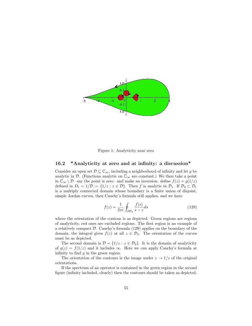
Figure 1: Analyticity near zero

16.2 *Analyticity at zero and at infinity: a discussion*

Consider an open set D ( C∞, including a neighborhood of infinity and let g beanalytic in D. (Functions analytic on C∞ are constant.) We then take a pointin C∞ \ D –say the point is zero– and make an inversion: define f(z) = g(1/z)defined in D1 = 1/D := 1/z : z ∈ D. Then f is analytic in D1. If D2 ⊂ D1

is a multiply connected domain whose boundary is a finite union of disjoint,simple Jordan curves, then Cauchy’s formula still applies, and we have

f(z) =1

2πi

∮∂D2

f(s)

s− zds (129)

where the orientation of the contour is as depicted. Green regions are regionsof analyticity, red ones are excluded regions. The first region is an example ofa relatively compact D. Cauchy’s formula (129) applies on the boundary of thedomain, the integral gives f(z) at all z ∈ D2. The orientation of the curvesmust be as depicted.

The second domain is D = 1/z : z ∈ D2. It is the domain of analyticityof g(z) = f(1/z) and it includes ∞. Here we can apply Cauchy’s formula atinfinity to find g in the green region.

The orientation of the contours is the image under z → 1/z of the originalorientations.

If the spectrum of an operator is contained in the green region in the secondfigure (infinity included, clearly) then the contours should be taken as depicted.

55

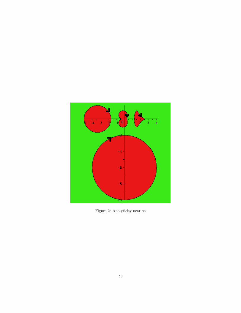
Figure 2: Analyticity near ∞

56

Assume as before that σ∞(T ) 6= C∞. Then there is a z0 ∈ C \ σ∞(T ) andwe assume without loss of generality that z0 = 0. We can define, as before, theset σ1 = 1/σ∞(T ) = 1/z : z ∈ σ∞(T ).

Then a function f is analytic on D ⊃ σ∞(T ) iff f(1/z) is analytic on σ1(T ).The spectrum σ∞(T ) is contained in D iff 1/D ⊃ 1/σ∞(T ). A curve, or setof curves, gives the value of f(T ) iff the curves are so chosen that 1/σ∞(T ) iscontained in the domain defined by the curves.

If f is nontrivial and analytic on σ∞(T ), then

Proposition 71. The Banach algebra of analytic functions on O with the supnorm is isomorphic to the algebra of bounded operators f [T ], in the operatornorm.

Proof. Linearity, continuity etc are proved as before. Multiplicativity could alsobe proved by density, taking say polynomials in 1/(z−z0), z0 /∈ σ(T ) as a denseset.

Alternatively, it could be proved directly from the definition (122) by Fubini.In any case, the analysis is rather straightforward and we leave all details to

the reader.

Finally,

Proposition 72. Assume σ∞(T ) = K+S (disjoint union) where K is compactin C. Let O ⊃ K be open, relatively compact and disjoint from S, and (w.l.o.g.)with rectifiable boundary C. Then

PK =1

2πi

∮C

1

z − Tdz (130)

defines a projector such that(i) PK(X) ⊂ D(T ), T (PK(X)) ⊂ PK(X).(ii) σ(T |PK(X)) = K.(iii) T restricted to PK(X) is bounded.

Proof. (Compare with §15.) Let P = PK ,χ = χK , First, we note that P =χ(T ) and χ is analytic on σ∞(T ), χ(∞) = 0 and thus, by Proposition 68 (i), PXis in D(T ). P 2 = P since χ2 = χ. Thus P is a projector, as in §15. By Prop.68 (ii) we have TP = (zχ)(T ) = (χz)(T ) = PT . Thus TP = TP 2 = PTP , andTPX ⊂ PX, and thus TP |PX ⊂ PX. We further have σ∞(TP ) = χ(σ∞(T )) =K. Since ∞ /∈ σ∞(TP ), TP is bounded.

16.3 Bounded self-adjoint and normal operators on a Hilbertspace H

Note 14. Assume A is bounded on the Hilbert space H and self-adjoint, thatis 〈Ax, y〉 = 〈x,Ay〉 ∀x, y ∈ H (this condition is not enough if A is unbounded).Then, by the Gelfand transform theory, σ(A) = K ⊂ R.

57

For a bounded operator to be self-adjoint, it suffices that it is symmetric,that is 〈Ax, y〉 = 〈x,Ay〉. Note that if A is self-adjoint, then ‖A2‖ = ‖A‖2.

From our excursion in Banach algebras we know that ‖A2‖ = ‖A‖2 (10)

and, more generally, ‖An‖ = ‖A‖n. Recall also that ‖A‖ = sup |σ(A)| = R(A).which holds more generally for normal operators.

17 Unbounded operators: adjoints, self-adjointoperators etc.

In this section we work with operators in Hilbert spaces.

1. Let H,K be Hilbert spaces (we will most often be interested in the caseH = K), with scalar products 〈, 〉H and 〈, 〉K.

2. T : D(T ) ⊂ H → K is densely defined if D(T ) = H.

3. Assume T is densely defined.

4. The adjoint of T is defined as follows. We look for those y for which

∃ v = v(y) ∈ H s.t.∀ x ∈ D(T ), 〈y, Tx〉K = 〈v, x〉H (132)

Since D(T ) is dense, such a v = v(y) is unique.

5. We define D(T ∗) to be the set of y for which v(x) exists ∀ x ∈ D(T ), anddefine T ∗(y) = v. Note that Tx ∈ K, y ∈ K, T ∗y ∈ H.

6. Check that D(T ∗) is a linear space and T ∗(a1y1 + a2y2) = a1T∗(y1) +

a2T∗(y2) that is, T ∗ is linear.

7. Definition. We write T1 ⊂ T2 iff D(T1) ⊂ D(T2), and T1 = T2 on D(T1).

Exercise 1. Show that T1 ⊂ T2 ⇒ T ∗2 ⊂ T ∗1 . (A short proof is given inCorollary 77.)

8.

Proposition 73. In the setting of 1 and 3, T ∗ is closed.

Proof. Let yn → y and T ∗yn → v. Then, for any x ∈ D(T ) we have

〈yn, Tx〉 =: 〈T ∗yn, x〉 → 〈v, x〉 = lim〈yn, Tx〉 = 〈y, Tx〉

Thus, for any x ∈ D(T ) we have 〈y, Tx〉 = 〈v, x〉 and thus, by definition,y ∈ D(T ∗) and T ∗y = v.

(10)Direct proof: with ‖u‖ = 1, we have

sup‖u‖=1

‖A2‖ > sup‖u‖=1

‖〈A2u, u〉‖ = sup‖u‖=1

‖〈Au,Au〉‖ = sup‖u‖=1

‖Au‖2 = ‖A‖2 (131)

. Since ‖A2‖ 6 ‖A‖2, the result follows.

58

9.

Proposition 74. Let T and D(T ) be as in 1 and 3. Then,

(i) For any α ∈ C, we have (αT )∗ = αT ∗.

(ii) If T ∈ L(H,K), then T ∗ is the usual adjoint, everywhere defined, andfor two such operators, we have (T1 + T2)∗ = T ∗1 + T ∗2 .

Proof. Exercise.

Proposition 75. (i) Let Ti and D(Ti) be as in 1 and 3. Assume further-more that D(T1)∩D(T2) is dense. Then (T1 +T2)∗ ⊃ T ∗1 +T ∗2 (this meansthat the domain is larger, and wherever all adjoints make sense, we have(T1 + T2)∗ = T ∗1 + T ∗2 ).

(ii) Let T1 : H → K1, T2 : H → K2 and assume D(T2) as well as D(T2T1)are dense. Then, (T2T1)∗ ⊃ T ∗1 T ∗2 .

Proof. We define T1 + T2 on D(T1) ∩D(T2). Let x ∈ D(T1) ∩D(T2) andassume that y ∈ D(T1)∗ ∩ D(T2)∗. This is, by definition, the domain ofT ∗1 + T ∗2 . Then

〈y, (T1 + T2)x〉 = 〈y, T1x+ T2x〉 = 〈y, T1x〉+ 〈y, T2x〉= 〈T ∗1 y, x〉+ 〈T ∗2 y, x〉 = 〈T ∗1 y + T ∗2 y, x〉 =: 〈(T1 + T2)∗y, x〉 (133)

and thus y ∈ D(T1 + T2)∗, and (T1 + T2)∗ = T ∗1 + T ∗2 .

(ii) Let x ∈ D(T2T1) (note that, by definition, D(T2T1) ⊂ D(T1)) andw ∈ D(T ∗1 T

∗2 ). Then,

〈T ∗1 (T ∗2w), x〉 = 〈(T ∗2w), T1x〉 = 〈w, T2T1x〉 (134)

and thus w ∈ D(T2T1)∗ etc.

17.1 Example: An adjoint of d/dx

There are much shorter ways to obtain the results in this section, but for prac-ticing with operators and adjoints, we will proceed here “the hard way”.

1. Let T = d/dx be defined on C1[0, 1]. We need to see for which y do wehave 〈y, Tf〉 = 〈w, f〉 ∀f ∈ D(T ), that is, ∀f ∈ D(T )∫ 1

0

y(s)df(s)

dsds =

∫ 1

0

w(s)f(s)ds

Let h(s) =∫ s

0w(t)dt. Then, h ∈ AC[0, 1]L2 := AC[0, 1] ∩ f : f ′ ∈

L2[0, 1] and we can integrate by parts∫ 1

0

y(s)df(s)

dsds =

∫ 1

0

dh(s)

dsf(s)ds = f(1)h(1)−

∫ 1

0

h(s)df(s)

dsds (135)

59

hence ∫ 1

0

(y(s) + h(s))df(s)

dsds = f(1)h(1) (136)

Let v ∈ C[0, 1] be arbitrary and take f =∫ x

1v. Then f ∈ C1[0, 1], f ′ = v

and f(1) = 0. Then, ∫ 1

0

(y(s) + h(s)) v(s)ds = 0 (137)

Note that the set of such v is dense. We can also set, for each v ∈ C[0, 1]f =

∫ x1v + 1. As before, f ∈ C1[0, 1], f ′ = v but now f(1) = 1. Thus,

also on a dense set, ∫ 1

0

(y(s) + h(s)) v(s)ds = h(1) (138)

Thus h(1) = 0. Also, by density, say from (137), y(s) + h(s) = 0. Nowh is by construction in AC[0, 1]L2 := AC[0, 1] ∩ f : f ′ ∈ L2[0, 1], andso is then y, h(0) = 0 and h(1) = 0 implies y(1) = y(0) = 0. Thus,D(T ∗) = AC[0, 1]L2

01 where the subscript 01 indicates that the functionvanishes at both ends. Clearly, on D(T ∗) we have (d/dx)∗ = −d/dx.

17.2 Symmetric does not mean self-adjoint

One property we certainly want to preserve is that σ(A) ⊂ R for a self-adjointoperator. Note that Ti = d/dx defined on f ∈ C1[0,∞]0 ∩ L2(R+) : f ′ ∈L2(R+), the subscript 0 indicating that the functions vanish at zero, is sym-metric on its domain, just by integration by parts. But note that, for λ > 0,iλ ∈ σ(T ), since f ′ − λf = g, f(0) = 0 has the unique solution f(x) =eλx

∫ x0e−λsg(s)ds, which is not everywhere defined (apply it to e−λs. So iλ ∈

σ(T ), and in fact, all λ with Imλ > 0 are in the spectrum.

17.3 Operations on graphs and graph properties

From now on, H and K are Hilbert spaces. Recall that H⊗K is a Hilbert spaceunder the scalar product

〈(x1, y1), (x2, y2)〉 = 〈x1, x2〉+ 〈y1, y2〉 (139)

1. Recall that the graph of an operator T is the set of pairs

G(T ) = (x, Tx) : x ∈ D(T ) ⊂ H ⊗K

Remember also that an operator T is closed iff G(T ) is a closed set, andit is closable iff the closure of G(T ) is the graph of an operator.

Exercise 2. If T is closable, then G(T ) = G(T )

60

17.3.1 A formula for the adjoint

1. Let us note something simple but very important. Assume y ∈ D(T ∗).Then

〈w, x〉H−〈y, Tx〉K = 0⇒ (−T ∗y, y) = V (y, T ∗y) = (−w, y) ⊥ (x, Tx)(140)

where V : K ⊗H → H⊗K is defined by

V (x, y) = (−y, x) (141)

Exercise 3. Compute the adjoint of V (in K⊗H) and show that V V ∗ =V ∗V = I, that is, V is unitary. Then V (E⊥) = (V (E))⊥ for any subspaceof K ⊗H. Clearly also, if mathcalH = K, then V 2 = −1.

Thus there is a simple link between G(T ) and G(T ∗):

Lemma 76 (Graph of the adjoint). We have

G(T ∗) = V [G(T )]⊥

Proof. Of course, (a, b) ⊥ G(T ) iff

∀x ∈ D(T ) : (a, b) ⊥ (x, Tx)⇔ 〈a, x〉 = 〈−b, Tx〉

that is, by definition, iff b ∈ D(T ∗) and b = −T ∗a. That is,

G(T )⊥ = (−T ∗a, a) : a ∈ D(T ∗)

andV (G(T ))⊥ = (a, T ∗a) : a ∈ D(T ∗) = G(T ∗) (142)

Corollary 77. T1 ⊂ T2 ⇒ T ∗2 ⊂ T ∗1 .

Proof. This follows from the reformulation above. Alternatively, D(T1) ⊂D(T2) and T1 = T2 on D(T ) means that D(T2)∗ ⊂ D(T1) and then fory ∈ D(T2)∗ and x ∈ D(T1) we have 〈T ∗2 y, x〉 = 〈y, T1x〉 = 〈T ∗1 y, x〉 etc.

From now on, we assume for simplicity that H = K.

2.

Theorem 18. Let T be densely defined. Then,

(i) T ∗ is closed.

(ii) T is closable iff D(T ∗) is dense, and then T = T ∗∗.

(iii) If T is closable, then the adjoints of T and of T coincide.

61

Proof. (i) By (142), T ∗ is closed (since its graph is closed).

(ii) Assume D(T ∗) is dense. Then T ∗∗ is well defined. By (142) its graphis given by

G(T ∗∗) = (VG(T ∗))⊥ = (V (V (G(T )))⊥)⊥

= (V 2G(T )⊥)⊥ = (G(T )⊥)⊥ = G(T ) (143)

and thus G(T ) is the graph of an operator. Since T ∗ is densely defined,T ∗∗ exists, and by Lemma 76 the left side of (143) is G(T ∗∗). Conversely,assume D(T ∗) is not dense. Let y ∈ D(T ∗)⊥ (y 6= 0); then (y, 0) isorthogonal on all vectors in G(T ∗), so that (y, 0) ∈ (G(T ∗))⊥. Then,V (y, 0) = (0, y) ∈ V (G(T ∗))⊥ = G(T ) by (143), and thus G(T ) is not thegraph of an operator.

(iii) We have by definition G(T ) = G(T ) and thus

G(T∗) = V [(G(T ))⊥] = V (G(T )

⊥) = G(T ∗) (144)

since E⊥=E⊥

for any E.

Proposition 78. Assume T is as in 4. Then (i) ker (T ∗) = ran (T )⊥ and (ii)ker (T )⊥ = ran (T ∗).

Proof. The proof is straightforward; it can be done from the graph approachor directly by interpreting the equality 〈T ∗y, x〉 = 0 = 〈y, Tx〉 where y spansker (T ∗) and x spans D(T ), or x spans ker (T ) and y spans D(T ∗). For instance

y ∈ ker (T ∗) ⇔ (y ∈ D(T ∗) and T ∗y = 0)

⇔ 〈T ∗y, x〉 = 0 = 〈y, Tx〉 ∀x ∈ D(T ) (145)

17.4 Self-adjoint operators

1. Assume now that K = H.

2. Definition: Symmetric (or Hermitian) operators. Let T be denselydefined on Hilbert space. T is symmetric if 〈Tx, y〉 = 〈x, Ty〉 for allx, y ⊂ D(T ). This means that T ⊂ T ∗.

3. A symmetric operator is always closable, by Theorem 18 since T ∗ isdensely defined, since T ∗ ⊃ T , by 2.

4. If T is closed, then G(T ) = G(T ) and thus by Theorem 18,

T = T ∗∗ (146)

62

5. Note that, if T is symmetric, then 〈Tx, x〉 ∈ R , since

〈Tx, x〉 = 〈x, Tx〉 = 〈Tx, x〉

and also, for any x ∈ D(T ), ‖(T ± i)x‖2 = ‖Tx‖2 + ‖x‖2, since

‖(T ± i)x‖2 = 〈Tx, Tx〉+ 〈x, x〉 ± 〈Tx, ix〉 ± 〈ix, Tx〉 = 〈Tx, Tx〉+ 〈x, x〉(147)

6.

Lemma 79. If T is symmetric and (assume already) closed, then (i)ran (T ± i) is closed and (ii) (T ± i) are injective.

Proof. (ii) Injectivity is immediate from (147) above.

(i) Let now (T ± i)xn be a convergent sequence, or, which is the same,a Cauchy sequence. But then, by (147) Txn and xn are both Cauchysequences. Then xn converges to x; since T is closed, x ∈ D(T ), andTxn → Tx.

Exercise 4. Note that ‖(T ± i)x‖ and the norm on the (closed) graphG(T ) coincide and that the space (0, ran(T±i)) is an orthogonal projection(P = P ∗) of G(T ± i). Provide an alternative proof of (i) based on this.

Definition: Self-adjoint operators. T is self-adjoint if T = T ∗. Itmeans D(T ) = D(T ∗), and T is symmetric.

7. It follows that self-adjoint operators are closed.

8. For self-adjoint operators we have from 4 that T = T ∗ = T ∗∗.

Lemma 80. If T is closed and symmetric and T ∗ is symmetric, thenT is self-adjoint.

Proof. By 2, T ⊂ T ∗. Since T ∗ is symmetric, T ∗ ⊂ T ∗∗ But T ∗∗ = Tsince T is closed, thus T ∗ ⊂ T , hence T ∗ = T .

17.5 The minimal and maximal operators based on d/dx:T0 and Tm

Note 15. The maximal domain of classical differentiation within L2[0, 1] definedas the functional inverse of the bounded operator

∫ x(see also the interesting

discussions in the chapter “The Fundamental Theorem of Calculus” in Rudin,Real and Complex analysis), (11) is Dm := AC[0, 1]L2 := f ∈ AC[0, 1] : f ′ ∈L2[0, 1]. Indeed, L2 ⊂ L1 and thus ran

∫ x:=

∫ xg : g ∈ L2 = Dm. We let

Tm be id/dx with D(Tm) = Dm.

(11)There are other possible definitions, s.a. through Fourier transform, and the domain ofthe operator will depend on the definition.

63

Define

T0 = id/dx on D(T0) = AC[0, 1]L201 := f ∈ AC[0, 1], f ′ ∈ L2[0, 1] : f(0) = f(1) = 0

(148)If x, y ⊂ D(T0), then a simple integration by parts shows that 〈y, T0x〉 =〈T0y, x〉, and thus T0 ⊂ T ∗0 .

The range of T0 consists of the functions of average zero, since∫ 1

0Ty = y|10 =

0 and conversely y = g′ has a solution g if∫ 1

0y = 0. Another way to phrase it

isranT0 = C⊥ (149)

Note 16. Similarly, ran (T0 ± i) = (e∓ixC)⊥.

Lemma 81. We have

T ∗0 = id/dx on D(T ∗0 ) = AC[0, 1]L2 (150)

First proof. Elementary analysis implies that f ′ convergent and f ′n(0) = 0 im-plies fn → f for some f and f(0) = 0 (likewise f(1) = 0). Thus T0 is closed.Tm is the maximal domain for id/dx and Tm = T ∗0 (easy to check), Tm is notsymmetric thus T0 is not self-adjoint (nor does it admit self-adjoint extensionsas we will see).

Second proof. Let τ be the operator in §??; we showed there that τ∗ = T0. ThusT0 is closed. We also proved before that τ is closed. Then τ = τ∗∗ = T ∗0 .

Direct proof. Assume that y ∈ D(T ∗0 ). Then, there exists a v ∈ L2[0, 1] suchthat for all x ∈ D(T0), we have

〈y, T0x〉 = 〈v, x〉 (151)

Since v ∈ L2[0, 1], we have v ∈ L1[0, 1], and thus h(x) =∫ x

0v(s)ds ∈ AC[0, 1]L2 ,

and h(0) = 0. With u = x, it follows from (151) by integration by parts that∫ 1

0

y(s)du(s)

ds= −

∫ 1

0

dh(s)

dsu(s)ds =

∫ 1

0

h(s)du(s)

ds

Let ϕ = y − h. By (149), we have∫ 1

0

ϕ(s)w(s)ds = 0 ∀w ∈ C⊥

This means that ϕ ∈ C⊥⊥ = C. Thus y is an element of AC[0, 1]L20 plus an

arbitrary constant, which simply means y ∈ AC[0, 1]L2 = D(T ∗0 ).

64

By essentially the same argument as in §??, we have T ∗∗0 = id/dx on D(T0).Thus T0 is closed. We note that T ∗0 is not symmetric. In some sense, T0 is toosmall, and then T ∗0 is too large.

Definition: Normal operators. The definition of an unbounded normaloperator is essentially the same as in the bounded case, namely, operators whichcommute with their adjoints.

More precisely: an operator T which is closed and densely defined is nor-mal if TT ∗ = T ∗T . The questions of domain certainly become very important.The domain if T ∗T is x ∈ D(T ) : Tx ∈ D(T ∗). (Similarly for TT ∗.) Thus,the operator T in (148) is not normal. Indeed, D(T ∗T ) consists of functionsin AC[0, 1]L2 vanishing at the endpoints, with derivative in AC[0, 1]L2 , whileD(TT ∗) consists of functions in AC[0, 1]L2 , with the derivative, in AC[0, 1]L2 ,vanishing at the endpoints.Definition: Essentially self-adjoint operators. A symmetric operator isessentially self-adjoint if its closure is self-adjoint. In the opposite direction, ifT is closed, then a core for T is a set D1 ⊂ D(T ) such that T |D1

= T .

Note 17. We will show that T ∗T and TT ∗ are selfadjoint (under domain con-ditions, of course), for any closed and densely defined T . If an operator Tis normal, then in particular D = D(T ∗T ) = D(TT ∗), and since D is dense andT is closed, we see that D is a core for both T and T ∗.

Note 18. By Corollary 77, if T1 ⊂ T2 and Ti are self-adjoint, then T1 = T2.Indeed, T1 ⊂ T2 ⇒ T1 = T ∗1 ⊃ T ∗2 = T2.

Lemma 82. (i) If T is essentially self-adjoint, then there is a unique self-adjointextension, T . (Phrased differently, if S ⊃ T is self-adjoint, then S = T ∗∗.)

(ii) (Not proved now). Conversely, if T has only one self-adjoint extension,then it is essentially self-adjoint.

Proof. (i) By definition T is selfadjoint. Let S be any self-adjoint extension ofT . By 7 above, S is closed. We have T ⊂ S ⇒ T ⊂ S = S. By the note 17.5above T = S.

Corollary 83. A self-adjoint operator is uniquely specified by giving it ona core.

Exercise 5. * Consider the operator T in §17.2. Is T closed? What is theadjoint of T? What is the range of T ± i?

1. A symmetric operator is essentially self-adjoint if and only if its adjoint isself-adjoint.

Indeed, assume T is e.s.a. and symmetric. Then T ∗∗ is s.a., and coincideswith all its successive adjoints. In particular T ∗ = T ∗ = T ∗∗∗ = T ∗∗.

Conversely, if T ∗ is s.a., then T := T ∗∗ = T ∗ which is self-adjoint.

65

Lemma 84. If T is self-adjoint, then ker (T ± i) = 0.

Proof. Compare with Lemma 79.

Theorem 19 (Basic criterion of self-adjointness). Assume that T is sym-metric.

Then the following three statements are equivalent:

(a) T is self-adjoint

(b) T is closed and ker (T ∗ ± i) = 0.(c) ran (T ± i) = H. More generally, if (a, b) ∈ R2 and b 6= 0 then

ran (T + a+ ib) = H(d) σ(T ) ⊂ R

Of course (we can take) D(T ± i) = D(T ). Remember the operator T in§17.2: it follows from (c) that T is not s.a.

Proof. (a)⇒ (b) is simply Lemma 84.

(b)⇒ (c): T is symmetric, thus T ∗ ⊃ T is densely defined and closed, thus,Proposition 78 above implies the result. The generalization is immediate,since aT/b is symmetric and closed as well. This implies in particular,since T is closed, that T + a+ ib is invertible, proving (c).

(c)⇒ (a) Let y ∈ D(T ∗). We want to show that y ∈ D(T ). By definition,for such a y,

〈y, (T + i)x〉 = 〈(T + i)∗y, x〉

Since ran (T − i) = H, there is an s ∈ D(T ) s.t.

(T + i)∗y = (T − i)s

for some s ∈ D(T ). Thus, since x ∈ D(T ) and since T is symmetric, wehave

〈y, (T + i)x〉 = 〈v, x〉 = 〈(T − i)s, x〉 = 〈s, (T + i)x〉 (152)

Now we use the fact that ran (T + i) = H to conclude that s = y. But swas in D(T ) and the proof is complete.

Corollary 85. Let T be symmetric. Then, the following are equivalent:

1. T is essentially self-adjoint.

2. ker (T ∗ ± i) = 0.

3. ran (T ± i) are dense.

66

Example 86. We know already that T0 is not s.a., nor e.s.a since it is alreadyclosed. Let’s however pretend we don’t have this argument, and use instead theabove criteria.

The range of T0 (see (149)) and Corollary 85 show that T0 is symmetric(thus closed since D(T0) is dense), but not essentially self-adjoint. Also, wenote that ker (T ∗0 ± i) 6= 0. Indeed,

idϕ

dx± iϕ = 0⇒ ϕ = Ce∓x

17.5.1 All self-adjoint extensions of id/dx on [0, 1]

Lemma 87. If T = id/dx defined on a dense domain in AC[0, 1]L2 then T isself-adjoint iff D(T ) = AC[0, 1]L2

ϕ where AC[0, 1]L2ϕ = f ∈ AC[0, 1], f ′ ∈ L2 :

f(0) = eiϕf(1), ϕ ∈ [0, 2π).

Proof. We need ran (T ±i) = H which means, by solving the ODEs (T ±i)f = gthat

∀g ∈ L2[0, 1],∃C = C(g) s.t. Ce±x +

∫ x

0

g(s)ds ∈ D(T ) (153)

solves the ODE for any C so the range is dense. This is one condition. Theother one is of course symmetry, and we have C to try to arrange this. Byintegration by parts

∫ifg =

∫fig iff ∀f, g ∈ D(T ), denoting f0 = f(0) etc. we

havef0g0 + f1(−g1) = 0 (154)

or

〈u, σv〉C = 0, σ =

(1 00 −1

)∀(u, v) ∈ E (155)

where E is a subspace of C2 and 〈u, σv〉C is the usual scalar product in C2.Clearly σ2 = 1, σ is self-adjoint and thus by the polarization identity it isequivalent to satisfy (155) when v = u. Since for a 6= 0 (a, 0) /∈ E , E 6= C2 andit is a zero or one dimensional subspace. If it is zero-dimensional, then E = 0,which would give us T = T0, D(T0) = AC([0, 1])01 on which we know T is notself-adjoint. Let then (1, α) generate E . It is immediate to check that |α| = 1and thus α = eiϕ for some ϕ. That this ϕ is independent of the f having f0,1

given follows from the fact that otherwise |f21 | = ei(ϕ1−ϕ2)|f1|2.

T0 is called the minimal operator associated to id/dx, T ∗0 is the maximaloperator. We see that T ∗0 has as spectrum C∞ (since eas is an eigenvalue forany a); T ∗0 is already a bit “too large”).

18 Extensions of symmetric operators; Cayleytransforms

Overview: The Cayley transform of a bounded self-adjoint operator, U = T−iT+i

is unitary (by functional calculus). This will be the case of unbounded s.a.

67

operators as well. Note meanwhile that (z−i)/(z+i) maps C into D. Conversely,we will show that unitary operators such that 1 − U is injective generate self-adjoint operators. Thus self-adjoint operators can be fully analyzed if we simplyunderstand unitary operators! Of course, more careful proofs are needed, andthey follow below.

Partial isometries are used to measure self-adjointness, find whether self-adjoint extensions exist, and find these extensions.

1. Let H± be closed subspaces of a Hilbert space H.

2. Definitions

(a) Recall that a unitary transformation Up from H+ to H− is called apartial isometry.

(b) The dimensions of the spaces (H±)⊥, finite or infinite, are calleddeficiency indices.

3.

Lemma 88. Let Up by a partial isometry. Then Up extends to a unitaryoperator on H iff the deficiency indices of Up are equal.

Proof. This is straightforward: assume the deficiency indices coincide.Two separable Hilbert spaces are isomorphic iff they have the same di-mension. Let U⊥ be any unitary between (H±)⊥. Let U = Up. We writeH = H+⊕(H+)⊥ and H = H−⊕(H−)⊥ and define U = Up⊕U⊥. Clearlythis is a unitary operator.

Conversely, let U is a unitary operator that extends Up. Then U(H+⊥) =(U(H+))⊥ = (Up(H

+))⊥ = H−⊥, and in particular H+⊥ and H−⊥ havethe same dimension.

4. In the steps below, T is closed and symmetric.

5. By Lemma 79 H± = ran (T ± i) are closed, and T ± i are one-to-one ontofrom D(T ) to H±.

Lemma 89. The operator (T − i)(T + i)−1 is well defined and a partialisometry between H+ and H−.

Note 19. The partial isometry (T − i)(T + i)−1 is known as the Cayleytransform of T .

By 5, Up = (T − i)(T + i)−1 is well defined on H+ with values in H−, andalso, for any u− ∈ H− there is a unique f ∈ D(T ) such that (T−i)f = u−.With u+ ∈ H+, we have Upu

+ = u−. Since ‖u−‖ = ‖(T − i)f‖ and(T + i)−1u+ = f, that is u+ = (T + i)f , we have ‖u±‖2 = ‖f‖2 + ‖Tf‖2.

68

Lemma 90. x ∈ D(T ) iff x = y − Upy for some y ∈ H+, i.e., D(T ) =ran (1− Up).

Proof. Note that on the range of T + i we have

1− Up = (T + i)(T + i)−1 − (T − i)(T + i)−1 = 2i(T + i)−1

and the result follows easily.

18.1 Duality between self-adjoint operators and unitaryones

Lemma 91. (i) If U is unitary and ker (1− U) = 0 (12), then there exists aself-adjoint T such that U = (T − i)(T + i)−1.

(ii) Conversely, if T is symmetric, then T is self-adjoint iff its Cayley trans-form is unitary on H.

Proof. 1. We start with (ii). Since T is s.a., T ± i are invertible, and inparticular ran (T ± i) = H, and σ(T ) ⊂ R. By the above, (T − i)(T +i)−1H → H, since D(T − i)−1 = ran (T + i) = H. We have alreadyshown that (T − i)(T + i)−1 is an isometry wherever defined, thus inthis case it is unitary. Conversely, U = (T − i)(T + i)−1 is defined onH, thus ran (T + i) = H and it since it is an isometry, it follows that(T − i)D (T ) = (T − i)(T + i)−1H = H thus ran (T ± i) = H.

2. We now prove (i). Note that ker (1−U) = ker (1−U∗). Indeed, x = Ux⇔U∗x = x. Let T = i(1 + U)(1− U)−1. Then T is defined on ran (1− U),which is dense in H, since ran (1− U)⊥ = ker (1− U∗) = 0.Now we want to see that for all x, y ⊂ D(T ) we have 〈x, Ty〉 = 〈Tx, y〉.

3. Note first that ran (1−U) = (1−U)H = −U(U∗ − 1)H = Uran (1−U∗).

4. Let x ∈ D(T ). Symmetry: x ∈ D(T ) is, by the above, the same as

x = U(U∗ − 1)z = (1− U)z; (and z = (1− U)−1x) (156)

Thus, to determine the adjoint, by (156) we analyze the expression 〈x, Ty〉where we first show T is symmetric. Let x, y ∈ D(T ). Then,

〈x, Ty〉 := 〈U(U∗ − 1)z, i(1 + U)(1− U)−1y〉〈Uz, i(U − 1)(1 + U)(1− U)−1y〉 = 〈Uz,−i(1 + U)y〉 = 〈i(1 + U∗)Uz, y〉

= 〈i(U + 1)z, y〉 = 〈i(U + 1)(1− U)−1x, y〉 = 〈Tx, y〉 (157)

(12)Or, equivalently, ran (1− U) is dense. This condition is needed to ensure D(T ) is dense,see Lemma 90.

69

5. Let’s check the range of T + i. We have D(T ) = ran (1− U), and thus

(T+i)D(T ) = (T+i)(1−U)H = i(1+U)(1−U)−1(1−U)H+i(1−U)H= i(1 + U)H+ i(1− U)H = 2iH = H (158)

Likewise, ran (T − i) = H.

18.2 Von Neumann’s Theorem on self-adjoint extensions

Theorem 20. Let T be a closed, densely defined, symmetric operator. ThenT has a self-adjoint extension iff the deficiency indices of its Cayley transformare equal.

Proof. (i) Assume Te is a self-adjoint extension of T . Let U = (T − i)(T + i)−1

and Ue = (Te − i)(Te + i)−1. By Lemma 91, Ue is unitary. We want to showthat Ue is an extension of U . Remember U : H+ → H−. Let x ∈ H+, thenx = (T + i)f = (Te+ i)f and Uex = (Te− i)f = (T − i)f = (Te− i)(Te+ i)−1x =Ux. Since U admits a unitary extension, then the deficiency indices are equal,see Lemma 88.

(ii) Conversely, assume that H± have the same dimension. Then there is aunitary Ue extending U . We first need to show that 1− Ue is injective. If thiswere not the case, and z ∈ ker (1 − Ue), thus, as before, z ∈ ker (1 − U∗e ) thusz ∈ ran (1− Ue)⊥ ⊂ ran (1− U)⊥ = D(T )⊥ = 0.

The rest of the proof is quite similar to that of (i). Let Te = i(1 + Ue)(1 −Ue)−1, a self-adjoint operator. We want to show that Te ⊃ T . Ue is defined on

ran (T+i) and D(Te) = ran (1−Ue). If x ∈ D(T ), then x = (1−U)y = (1−Ue)yfor some y and thus Tx = i(1+U)(1−U)−1x = i(1+Ue)(1−Ue)−1x = Tex

Corollary 92. Let T be symmetric and closed. Then T has a self-adjointextension iff ker (T ∗ − i) and ker (T ∗ + i) have the same dimension, that is, iffran (T ± i)⊥ have the same dimension.

Exercise 1. Show that the symmetric operator in §17.2 has no self-adjointextension.

19 Spectral theorem: various forms

We first formulate the various forms of this theorem, then apply it on a numberof examples, and then prove the theorem.

19.1 Bounded operators

Theorem 21 (Functional calculus form (I)). Let A be a bounded self-adjointoperator on H, a separable Hilbert space. Then there exists a finite measure

70

space M,µ, a unitary operator from H onto L2(M,dµ) and a bounded func-tion F so that the image of A under U is the operator of multiplication by F .

That is A = U−1×FU , where (

×Ff)(ω) =: F (ω)f(ω).

Equivalently (the equivalence is simple, we’ll show it later).

Theorem 22 (Functional calculus form (II)). Let A be a bounded self-adjointoperator on H, a separable Hilbert space. Then there exists a decomposition

H = ⊕Nn=1Hn, N 6∞

so that, on eachHn, A is unitarily equivalent to multiplication by x on L2(R, dµn)

for some finite measure µn (meaning A = U−1×xU where×x(f(x)) = xf(x)).

That is, A is unitarily equivalent to multiplication by x. The measures dependon A, of course. The measures are thus non-canonical. Also, for any analytic f ,

f(A) = U−1×FU .

The measures dµn are called spectral measures.

19.2 Unbounded operators

Theorem 23. Let A be a self-adjoint operator on H, a separable Hilbert space.Then there exists a Radon measure space M,µ, a unitary operator from Honto L2(M,dµ) and a function F such that the image of A under U is the

operator of multiplication by F . That is A = U−1×FU . Also, ψ ∈ D(A) iff

F (ω)(Uψ)(ω) ∈ L2(M,dµ)).(Furthermore, the measure space can be arranged so that F ∈ Lp(dµ) for

any p ∈ [0,∞).)

19.2.1 Spectral projection form

Let A be selfadjoint. There is a family of orthogonal projections P associatedto A, with the following properties. For every measurable set S in R there is aprojection PS (the projection on the part S of the spectrum of A). They havethe following properties.

1. P∅ = 0, PR = I.

2. If S = ∪∞1 Sn (all sets being measurable) and Sn∩Sm = ∅ for n 6= m, thenPS = s− lim

∑∞1 Pn where s− lim is the strong limit.

3. PS1PS2 = PS1∩S2 .

Theorem 24 (Spectral projection form. This form is the same for boundedor unbounded operators). Let A be a self-adjoint operator. Then there existspectral projections as above, such that

A =

∫RλdPλ

71

For now, we understand (iv) in the sense

〈f,Ag〉 =

∫Rλd〈f, Pλg〉

where d〈f, Pλg〉 is a usual measure, as it is straightforward to check using theproperties of the family P .

Note 20. It is important to emphasize that, unlike the other forms of thespectral theorem, this representation is canonical: given A there is a uniquefamily of projections with the properties above.

Returning to our functional calculus, if g is analytic on the spectrum of A(contained in R, of course, containing infinity if the operator is unbounded),the image of g(A) is the function g(F ). But note that now we can defineeitA =

∫R e

itλdPλ for an unbounded A, while eix is certainly not analytic at ∞.

20 Proof of the functional calculus form

20.1 Cyclic vectors

Consider a bounded self-adjoint operator A, a vector ψ in H and the vectorsAnψn∈N. If we take all linear combinations of Anψ and then its closure, the“span” of Anψ denoted by

∨∞n=1A

nψ, is a Hilbert space Hψ. If ψ is such thatHψ = H, then ψ is a cyclic vector. Not all operators A have cyclic vectors.

Exercise 1. Which self-adjoint matrices have cyclic vectors?

Note that we can take any vector, form H[0] = Hψ and then pick a vectorin H⊥ψ and construct H[1], “etc.” (see the exercise below for the “etc.”)

Exercise 2. Show (for instance using Zorn’s Lemma) that every separableHilbert space can be written as

H = ⊕Nn=1HψN, N 6∞ (159)

where ψj is cyclic for Hψj.

Now, to prove Theorem 22 it suffices thus to prove it in eachHψN, or, w.l.o.g.,

assume that ψ is already cyclic for H. Of course, we can assume ‖ψ‖ = 1.We can define a functional L, first on analytic functions f on σ(A) by

L(f) = 〈f(A)ψ,ψ〉 (160)

L is bounded since

|L(f)| 6 ‖f(A)‖ = sup|f(λ)| : λ ∈ σ(A) = ‖f‖∞ (161)

(see Prop. 60 above, p. 46, (131), and Exercise 4 on p. 58.

72

On the other hand, this is a positive functional, since if f is positive (13) onσ(A) then f = g2 with g analytic too and real valued, and thus

〈f(A)ψ,ψ〉 = 〈g(A)2ψ,ψ〉 = 〈g(A)ψ, g(A)ψ〉 = ‖g(A)ψ‖2 > 0 (162)

Since analytic functions on a compact set in R, σ(A), are dense in C(σ(A))(polynomials are already dense) and the functional f 7→ 〈f(A)ψ,ψ〉 is positiveand of norm one on a dense subset, it extends to C(σ(A)) and, by the Riesz-Markov theorem, there is a measure dµψ so that

〈f(A)ψ,ψ〉 =

∫σ(A)

fdµψ(x) (163)

Note the dependence on ψ; see Note 30 below for a physical interpretation ofµψ(x). For simplicity however, we drop the subscript ψ : µ = µ. We cannow consider HA = L2(σ(A), dµ). We want to define a unitary transformationbetween H and HA. (Note that up to now we showed bounds between H andL∞(σ(A)).)

It is more convenient to define U on HA with values in H. The vectors inHA are of course functions on σ(A). From (163) we expect ϕ to be mapped intoϕ(A)ψ. Define thus for f analytic (not necessarily real-valued) on σ(A),

Uf = f(A)ψ (164)

Remember (see p. 54) that

f(A)∗ = f∗(A) and for x ∈ R we have f∗(x) = f(x) (165)

Therefore ∫|f |2dµ (163)

= 〈f(A)(f(A))∗ψ,ψ〉 = ‖f(A)ψ‖2 = ‖Uf‖2 (166)

Thus the transformation U , defined on a dense subset of L2(σ(A), dµ) extendsto an isometry from L2(σ(A), dµ) into H.

We only have to check that indeed the image U−1AU of A is the operatorof multiplication by the variable. We have for analytic f ,

Uf := f(A)ψ ⇒ U−1AUf = U−1Af(A)ψ = U−1Af(A)ψ

= U−1(×xf×)(A)ξ = U−1U

×x×f =

×xf (167)

Since (167) holds on a dense set, the proof is complete.

Note 21. Whether ψ is cyclic or not, formulas (164) and (166) above allow us todefine any L2 functions of A. Indeed, analytic functions (or even polynomials)are dense in L2. If fn → h in the sense of L2, then fn(A)ψ converges to (by

(13)Not merely nonnegative.

73

the definition of fn(A)) h(A)ψ. Thus we can define, given ψ arbitrary, h(A)ψfor any h ∈ L2. It is easy to check that h is bounded and linear: Indeed, if ψ iscyclic for the whole of H there is essentially nothing to show. If it is not, thenit is correctly defined and bounded on each Hn with values in Hn while Hn aremutually orthogonal. Simply define h(a)x =

∑h(A)xn where (xn)n6N is the

orthogonal decomposition of x. Now, if h = χS , the characteristic function of ameasurable set, then χS(A), is, of course, a spectral projection.

Note 22. Note that (161) shows that if we take the closure in the operatornorm of A(A) := f(A) : f analytic on σ(A) then we get C(A) the continuousfunctions on σ(A). In Note 21 we have taken the strong-limit closure of A(A),since convergence of fn is only used pointwise– convergence of fnψ for any ψ.This gives us in particular M(A), the bounded measurable functions on σ(A),applied to A. Compare also with what we have done in §11. The apparentsimilarity can be misleading.

Note 23. Note also that we have made substantial use of the fact that A wasself-adjoint to define M(A) (for instance, in using (165)).

21 Examples: The Laplacian in R3

Most of this section is based on [6], where more results, details, and examplescan be found.

In a number of cases, the unitary transformation mapping an unboundedself-adjoint operator T to a multiplication operator is explicit. Then, we canuse the exercise below to find all information about T .

Exercise 1. Show that, if U is unitary between H1 and H2, then T is self-adjoint on D(T ) ⊂ H1 iff UTU−1 = UTU∗ is self-adjoint in UD(T ).

As an example, consider defining −∆ in R3. Define it first on D0(∆) = C∞0where it is symmetric. Let U be the Fourier transform, a unitary operator. Itis in fact easier to work with another set of functions, still dense in L2(R3) ascan be easily checked, which admit an explicit Fourier image:

D1 =e−x

2/2P (x) : P polynomial

(168)

This is Fourier transformed to

UD1 =e−k

2/2P (k) : P polynomial

(169)

Exercise 2. Check that D1 is dense in L2(R3). Check that on D1 T is sym-metric and that UT (f) = |k2|Uf , a multiplication operator.

We will denote |k2| by k2 and Uf by f .

Exercise 3. Check that k2 is self-adjoint on

D(k2) = f ∈ L2(R3) : k2f ∈ L2(R3) = f : (k2 + 1)f ∈ L2(R3) (170)

74

Thus, we have

Proposition 93. −∆ is self-adjoint on U−1D(k2). Call this operator H0.

The characterization of D(H0) is simplest through Fourier transform. Thisgives another dimension to the need for Sobolev spaces etc.

Let u ∈ D(H0) and u be its Fourier transform. A direct space characteriza-tion is more difficult, though we might simply say that u together with all secondorder partial derivatives exist as weak derivatives, in distributions (equivalently,defined in L2 as as inverse Fourier transforms of kikj u), and the derivatives arein L2.

We can see some classical properties of elements of u ∈ D(H0). We can showthat u is bounded and uniformly continuous as follows. Noting that both u andk2u are in L2 it follows immediately that (α2 + |k|2)u ∈ L2 for any α. This is,essentially by definition the Sobolev space H2(R3). Let k = |k| and dk be theLebesgue measure on R3.

For boundedness, we use Cauchy-Schwarz:(∫R3

|u|dk)2

6∫R3

dk

(k2 + α)2

∫R3

[(k2 + α)|u|]2dk =π2

α‖(H0+α)u‖2 <∞

(171)

Note also that|eik·x − eik·y| 6 max2, k|x− y| (172)

Similarly, we can calculate that, if β < 1/2, then

|u(x)− u(y)| 6 Cβ |x− y|β(α−(1/2−β)‖H0u‖+ α3/2+β‖u‖

)(173)

which easily implies that u is Holder continuous with any exponent < 1/2.However, u is not even once classically differentiable!

The inequalities (171) and (173) are special cases of Sobolev inequalities.For more details and examples, see [6], pp. 299.Here is a very useful and general criterion of self-adjointness, in the un-

bounded case. First, a definition:

Definition 94. (i) An operator A is relatively bounded with respect to T (T−bounded)if D(A) ⊃ D(T ) and for some a, b and all u ∈ D(T ) we have

‖Au‖ 6 a‖u‖+ b‖Tu‖ (174)

An equivalent condition is that for some (different) a′, b′ we have

‖Au‖2 6 (a′)2‖u‖2 + (b′)2‖Tu‖2 (175)

The equivalence of (174) and (175) is left as an exercise (details are given in[6], p. 287, but the exercise is simple enough). (ii) The T−bound is defined asthe greatest lower bound of the b for which there is an a so that (174) holds, orequivalently the greatest lower bound of the b′ for which there is an a′ so that(175) holds.

75

Theorem 25 (Kato-Rellich). Let T be self-adjoint. If A is symmetric andT−bounded with T−bound b′ < 1 then T + A is self-adjoint. This is the casein particular if A is bounded.

Proof. First, it is clear that D(T + A) = D(T ) and T + A is symmetric. Wewill show that (c) in Theorem 19 holds. Without loss of generality we take alsoa′ > 0. Recall (147). This implies immediately that

‖Ax‖ 6 ‖(b′T ∓ ia′)x‖, (x ∈ D(T )) (176)

Denote c′ = a′/b′ and (T ∓ ic′)x = y, and recall Theorem 19 (b) (c). Thisimplies that

R(∓ic′) def=(T ∓ ic′)

exist and are bounded. Thus

‖AR(∓ic′)y‖ 6 b′‖y‖, (x ∈ D(T )) (177)

In particular (again by Theorem 19 (b) (c)) this means that

B± = −AR(∓ic′) are bounded and ‖B±‖ < b′ < 1 (178)

Therfore, by the standard Neumann series argument, (1−B±)−1 exist and arebounded (with norm 6 1/(1− b′)) and thus (1−B±) are bounded and one-to-one. Note now that T ∓ ic′ is one to one, so is (1−B±) and thus their productis one-to-one.

(1−B±)(T ∓ ic′) = T ∓ ic′ +AR(∓ic′)(T ∓ ic′) = T ∓ ic′ +A (179)

Thus ran (T+A∓ic′) = ran 1c′ (T+A)∓i = H and thus T+A is self-adjoint.

Example The operator−∆+V (x) is self-adjoint onD(−∆) for any boundedreal function V . This follows trivially from Theorem 25.

In one dimension, say on L2[0, 1], for any bounded, measurable, real f ,id/dx + f(x) (or −d2/dx2 + f(x)) are self-adjoint on any domain on whichid/dx (or −d2/dx2) is self-adjoint. Find self-adjointness domains for −d2/dx2.

More generally, one can show (see [6]) the following.

Proposition 95 ([6], p. 302). Consider functions of the form q = q0 +q1 whereq0 ∈ L∞(R3) and q1 ∈ L2(R3). Then

−∆ + q (180)

is essentially self-adjoint on C∞0 (R3) and self-adjoint on D(−∆).

Example q = 1/r, r = |x| satisfies the assumptions of Proposition 95. Thusthe Hamiltonian of the Coulomb atom,

−∆ + e/r (181)

is self-adjoint on D(H0).

76

22 A few more facts about compact operators

Proposition 96. If A,B are as in Theorem ?? and A−1 is compact and B isbounded, then (A+B)−1 is compact.

This is immediate from the second resolvent formula.

Corollary 97. Let T = id/dx+ V (x) on AC[0, 1] with periodic boundary con-ditions, where V (x) is real valued and bounded. Then T is self-adjoint withcompact resolvent.

Proof. This follows from Theorem 25 and the second resolvent formula, Theorem??.

23 Equivalence with Theorem 21

For that we simply take N copies of R, take their disjoint union M = ∪Nn=1Rand on each copy we take a vector of norm 2−n. Then we take the measureµ = ⊕µn on M , and clearly µ(M) <∞. The rest is immediate.

24 Extension to Borel functions of A

Since A corresponds to multiplication by a function F , if h is any boundedBorel measurable function on σ(A) we define h(A) = Uh FU−1, wheneverh F exists in the underlying Hilbert space. In particular, if h is chosen tobe χS , the characteristic function of a subset S, then PS = UχSU−1 is anorthogonal projection, in fact a spectral measure. We want to see that

A =

∫xdP (x)

Let S be an arbitrary measurable subset of σ(A) ⊂ R and define, for each pairx, y ∈ H,

ν(S) = 〈Psx, y〉

Then,

25 Defining self-adjoint operators

Suppose A is symmetric, and that we can find a unitary transformation Uthat maps H into L2(R, dµ) in such a way that A is mapped onto a· for allψ ∈ D(A), and that means that a· is initially defined on U(D(A)) which is alsodense, since U is unitary. Then, clearly, (A± i)−1 are mapped to (a± i)−1, since(A± i)(A± i)−1 = 1 on D(A). It is clear that Ua = (a ·−i)(a ·+i)−1, the imageof UA = (A−i)(A+i)−1 is extends to a unitary operator on UD(A) = UH. Butthis does not mean that it was unitary to start with, since it was only definedon (a+ i)f : f ∈ UD(A) which may not be dense in L2(R, dµ).

77

Nevertheless, Ua extends to a unitary operator, and thus UA extends to aunitary operator, and thus A has some self-adjoint extension A1, (canonical wrtthis particular construction...). What is the domain of A1? This can be writtenin terms of UA: D(A) = ran (UA−1), which is simply U−1ran (ua−1) = D(a·).On the other hand, this is simple to calculate, it consists of the functions g suchthat

D(a) =g ∈ L2(R, dµ) :

∫R|g|2a2da <∞

(182)

Exercise 1. Apply these arguments to A = id/dx defined originally on C∞0 ,using as U the discrete Fourier transform and, as usual k instead of a as adiscrete variable. What is UD(A)? On UD(A) k· is simply multiplication byk. The domain of the adjoint is larger than the set of sequences ckk∈Z withkck ∈ L2. What is it? Find a self-adjoint extensions of A. Can you find morethan one?

Thus,

D(A) = U−1g ∈ L2(R, dµ) :

∫R|g|2a2da <∞

(183)

26 Spectral measures and integration

We have seen that finitely many isolated parts of the spectrum of an operatoryield a “spectral decomposition”: The operator is a direct sum of operatorshaving the isolated parts as their spectrum. Can we allow for infinitely manyparts?

We also saw that, if the decomposition of the spectrum is K1 + K2, whereχ1χ2 = 0, then the decomposition is obtained in terms of the spectral projec-tions Pi = χi(T ) where P1P2 = 0 and P1 +P2 = I. We can of course reinterpret(probability-)measure theory in terms of characteristic functions. Then a mea-sure becomes a functional on a set of characteristic functions such that χiχj = 0(the sets are disjoint) then

χ(

∞⋃i=1

Ai) =

∞∑k=1

χi

andχ(A1 ∩A2) = χ1χ2

In terms of measure, we then have

µ(

∞∑k=1

χk) =

∞∑k=1

µ(χk)

µ(1) = 1

(continuity of the functional) etc.In the following, we let Ei := E(Ai).

78

Note 24. 1. In a Hilbert space it is natural to restrict the analysis of pro-jectors to orthogonal projections. Indeed, if H1 ( H is a closed subspaceof H, itself then a Hilbert space, then any vector x in H can be written inthe form x1 + x2 where x1 ∈ H1 and x2 ⊥ x1. So to a projection we canassociate a natural orthogonal projection, meaning exactly the operatordefined by (x1 + x2)→ x1.

2. An orthogonal projection P is a self-adjoint operator. Indeed,

〈Px, y〉 = 〈x1, y1 + y2〉 = 〈x1, y1〉 = 〈x1 + x2, y1〉 = 〈x, Py〉

3. Conversely, if P is self-adjoint, and x = x1 + x2, where Px1 = x1, then

〈x1, x2〉 = 〈Px, (1− P )x〉 = 〈x, P (1− P )x〉 = 0

Let Ω be a topological space, BΩ be the Borel sets on Ω and A(H) be the self-adjoint bounded operators on the Hilbert space H: ∀(x, y), 〈Tx, y〉 = 〈x, Ty〉.Thus, with Ai ∈ BΩ, the spectral projections E := χ(T ) should satisfy

1.

(∀i 6= j, Ai ∩Aj = ∅) ⇒ E(

∞⋃i=1

Ai)x =

∞∑k=1

Eix

2.E((A1 ∩A2) = E1E2

3.E(Ω) = I; E(∅) = 0

Definition 98. A projector valued spectral measure on BΩ with values in A(H)is a map E : BΩ → H with the properties 1,2,3 above.

Note 25. E(A) is always a projector in this case, since E(A) = E(A ∩ A) =E(A)2 and E(A)E(B) = E(B)E(A) since they both equal E(A ∩B).

Proposition 99 (Weak additivity implies strong additivity). Assume 2. and3. above, and that for all (x, y) ∈ H2 we have

(∀i 6= j, Ai ∩Aj = ∅) ⇒ 〈E(

∞⋃i=1

Ai)x, y〉 = 〈∞∑k=1

Eix, y〉

Then 3. above holds.

Remark 26. Note a pitfall: we see that

E(

∞⋃i=1

Ai)x =

∞∑k=1

Eix (184)

for all x. But this does not mean that∑Ni=1Eix converge normwise!

79

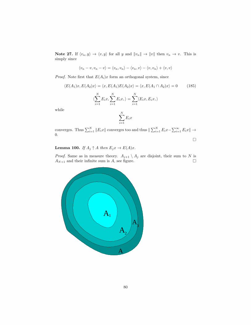
Note 27. If 〈vn, y〉 → 〈v, y〉 for all y and ‖vn‖ → ‖v‖ then vn → v. This issimply since

〈vn − v, vn − v〉 = 〈vn, vn〉 − 〈vn, v〉 − 〈v, vn〉+ 〈v, v〉

Proof. Note first that E(Ai)x form an orthogonal system, since

〈E(A1)x,E(A2)x〉 = 〈x,E(A1)E(A2)x〉 = 〈x,E(A1 ∩A2)x〉 = 0 (185)

〈N∑i=1

Eix,

N∑i=1

Eix, 〉 =

N∑i=1

〈Eix,Eix, 〉

whileN∑i=1

Eix

converges. Thus∑Ni=1 ‖Eix‖ converges too and thus ‖

∑Ni=1Eix−

∑∞i=1Eix‖ →

0.

Lemma 100. If Aj ↑ A then Ejx→ E(A)x.

Proof. Same as in measure theory. Aj+1 \ Aj are disjoint, their sum to N isAN+1 and their infinite sum is A, see figure.

A1

A2

A3

A

80

27 Integration wrt projector valued measures

Let f be a simple function defined on S ∈ BΩ. This is a dense set in B(Ω,C).

f(ω) =

N∑i=1

fjχ(Sj) (186)

As usual, Si ∩ Sj = ∅ and ∪Si = S. Then we naturally define∫S

f(ω)dE(ω) =

N∑i=1

fjE(Sj) (187)

This is the usual way one defines integration wrt a scalar measure.

Note 28. We note an important distinction between this setting and that of§11: here we integrate scalar functions wrt operator valued measures, whereasin §11 we integrate operator-valued functions against scalar measures.

Note 29. (14) In §11 as well as in the few coming sections, we restrict ourselvesto integrating uniform limits of simple functions. The closure in the sup normof simple functions are the measurable bounded functions, which is not hardto verify, so this is a more limited integration than Lebesgue’s (e.g., L1 is notaccessible in this way.)

It is also interesting to note the following theorem:

Theorem 26 (Sikic, 1992). A function f is Riemann integrable iff it is theuniform limit of simple functions, where the supporting sets Ai are Lebesguemeasurable with the further property that µ(∂Ai) = 0.

Without the restriction on µ(∂Ai), the closure of simple functions in the supnorm is the space of bounded measurable functions (exercise).

Proposition 101. The definition (187) is independent of the choice of Sj, fora given f .

Proof. Straightforward.

Proposition 102. The map f →∫Sf is uniformly continuous on simple func-

tions, and thus extends to their closure. We have∥∥∥∥∫S

f(ω)dE(ω)

∥∥∥∥ 6 supS|f(ω)| (188)

Proof. We can assume that the sets Si are disjoint. Then the vectors Eix areorthogonal and∥∥∥∥∫

S

f(ω)dE(ω)

∥∥∥∥2

=

N∑i=1

fi‖E(Si)x‖2 6 supS|f |2

N∑i=1

〈Eix, x〉 6 supS|f |2‖x‖2

(14)Pointed out by Sivaguru Ravisankar.

81

Consider then the functions in B(Ω,C) which are uniform limits of simplefunctions. The integral extends to B(Ω,C) by continuity and we write∫

S

f(s)dE(s) := limn→∞

∫S

fn(s)dE(s) (189)

Definition 103. A C∗-algebra is a Banach algebra, with an added operation,conjugation, which is antilinear and involutive ((f∗)

∗= f) and ‖f∗f‖ = ‖f‖2.

Exercise 1. Show that ‖f∗‖ = ‖f‖.

Proposition 104. f 7→∫Sf(ω)dE(ω) is a C∗-algebra homeomorphism.

Proof. We only need to show multiplicativity, and that only on characteristicfunctions, and in fact, only on very simple functions, where N = 1, and thecoefficients are one. We have∫

χ(S1)χ(S2)dE(S) = E(S1 ∩ S2) = E(S1)E(S2) (190)

Exercise 2. Complete the details.

27.1 Spectral theorem for (unbounded) self-adjoint oper-ators

Theorem 27. Let A be self-adjoint. There is a spectral measure on the Borelσ-algebra of R such that

Ax =

∫RtdE(t)x := lim

∫ k

−ktdE(t)x (191)

for all x ∈ D(A). Furthermore,

D(A) = x ∈ H :

∫Rt2d〈E(t)x, x〉 <∞ (192)

We know that self-adjoint operators are in a one-to-one correspondence withunitary operators. Assuming we have the spectral theorem for bounded normaloperators and u is a unitary operator, then we have

U =

∫C

udE(u) (193)

where C is the unit circle. Then, with A = i(1 + U)(1− U)−1 we expect

A =

∫C

i1 + u

1− udE(u) (194)

82

which we can formally write

A =

∫Rtd(E ϕ)(t) =

∫RtdE′(t) (195)

where

ϕ(t) =t− it+ i

(196)

and where E′(S) = E(ϕ(S)) is a new spectral measure.We have to ensure that the theory of integration holds, and that it is com-

patible with changes of variable, and to interpret the singular integrals obtained.

28 Spectral representation of self-adjoint and nor-mal operators

We first state the main results, which we will prove in the sequel.

Theorem 28 (Spectral theorem for bounded normal operators). Let N bebounded and normal (that is, NN∗ = N∗N). Then there is spectral measure Edefined on the Borel sets on σ(N), see Definition 98, such that

N =

∫σ(N)

zdE(z) (197)

Theorem 29 (Uniqueness of the spectral measure). Let N be a normal, boundedoperator.

(i) Assume E[1] and E[2] are spectral measures on the Borel sets on σ(N)such that

N =

∫σ(N)

zdE[1] =

∫σ(N)

zdE[2] (198)

Then E[1] = E[2].(ii) More generally, if Ω ∈ C ⊃ σ(N) is a closed set and E[3] is a spectral

measure on Ω such that

N =

∫σ(N)

zdE[3] (199)

Then E(Ω\σ(N)) = 0 and the Borel measure induced by E[3] on σ(N) coincideswith E, the spectral measure of N .

What can the spectrum of a normal operator be? Let D be a compact set inR2, and consider L2(D). Consider the operator Z := f(x, y) 7→ (x+ iy)f(x, y).Then Z∗ = f(x, y) 7→ (x − iy)f(x, y), and Z is a normal operator. Clearly, if(x0, y0) /∈ D and λ = x0 + iy0, then 1/(x + iy − λ) is bounded on D and it isthe inverse of (x + iy − λ); otherwise, if (x0, y0) ∈ D, then (x + iy − λ) has nononzero lower bound, and thus is not invertible. Then σ(Z) = D.

83

28.1 Spectral theorem in multiplicative form

Definition 105. A vector ψ ∈ H is cyclic for the (bounded) operator A if theclosure of the set of linear combinations of vectors of the form Anψ, n ∈ N(denoted by

∨∞n=1A

nψ) is H.

In this formulation, self-adjoint operators are unitarily equivalent with mul-tiplication operators on a direct sum of L2(σ(A)), dµn with respect to certainmeasures. If A has a cyclic vector, then the measure is naturally defined in thefollowing way. We know how to define bounded measurable functions of A (forinstance taking limits of polynomials). Then, 〈ψ, f(A)ψ〉 =

∫σ(A)

f(ω)dµψ(ω).

Note 30. In Quantum mechanics, if o (angular momentum, energy, etc.) isan observable, then it is described by a self-adjoint operator O. The spectrumof O consists of all possible measured values of the quantity o. An eigenvectorψa of O is a state in which the measured observable has the value o = a withprobability one.

If ψ is not an eigenvector, then the measured value is not uniquely deter-mined, and for an ensemble of measurements, a number of values are observed,with different probabilities. The average measured value of o or the expectedvalue of o, in an ensemble of particles, each described by the wave function ψis 〈ψ,Oψ〉.

Imagine that the measured quantity is χ[a,b](o). That is, if say o is the energy,then χ[a,b](o) is a filter, only letting through particles with energies between aand b (a spectrometer only lets through photons in a certain frequency range,and since E = hν, certain energies).

Then, 〈ψ,χa,b(E)ψ〉 is the expected number of times the energy falls in [a, b],that is, the density of states. This is a physical interpretation of dµψ.

Theorem 30. Assume A is a bounded self-adjoint operator with a cyclic vec-tor ψ. Then there is a unitary transformation U that maps H onto HA =L2(σ(A), dµψ) and A into the multiplication operator Λ = f(λ) 7→ λf(λ):

UAU−1 = Λ (200)

Note 31. This unitary transformation is non-canonical. But cyclicity meansthat the transformation ϕ 7→ Oψ is ergodic, mixing, and the measures areexpected to be equivalent, in some sense.

Clearly, uniqueness cannot be expected. L2([0, 1]) with respect to dx andwith respect to f(x)dx α < 0 < f < β are unitarily equivalent, and the unitarytransformation is g 7→

√fg. X, multiplication by x is invariant, since UXU−1 =

X. The measure is determined up to measure equivalence: two measures areequivalent iff they have the same null sets. Instead, the spectral projections areunique.

In case A does not have a cyclic vector, then H can be written as a finiteor countable direct sum of Hilbert spaces H = ⊕Nn=1Hn, N 6 ∞ such that

84

A|Hn has a cyclic vector ψn. Then, as before, there is a unitary transformationU : H → ⊕Nn=1L

2(R, dµn) so that

(UAU−1)Hn = Λ (201)

Let F be the operator g 7→ fg where f, g ⊂ L2(M,dµ). As a corollary,

Proposition 106. Let A be bounded and self-adjoint. Then, there exists a finitemeasure space (M,µ) (µ(M) <∞), a bounded function f on M and a unitaryoperator U : H → L2(M,dµ) so that

UAU−1 = F (202)

Like all other measures, µψ can be decomposed uniquely into three disjointmeasures: µpp + µac + µsing. Let µ be a finite measure on R.

(i) µpp (pure point). A measure is pure point, µpp if, by definition, for anyB ∈ Ω we have µ(B) =

∑ω∈B µ(ω). We note that the support of µpp is a

countable set, since the sum of any uncountable family of positive numbers isinfinite.

(ii) µac. A measure is absolutely continuous with respect to the Lebesguemeasure dx if, by definition, dµ = f(x)dx where f ∈ L1(dx).

(iii) A measure is singular with respect to the Lebesgue measure if there isa set S of full Lebesgue measure (R = S + S′ where S′ is a set of measure zero,and µ(S) = 0. Thus µsing is concentrated on a zero Lebesgue measure set.

(iv) Pure point measures are clearly singular. To distinguish further, we saythat a measure µ is continuous if µ(x) = 0 for any point x.

(v) µsing. A measure is singular continuous if µ is continuous and singularwith respect to the Lebesgue measure.

Decomposition theorem. Any measure µ on R has a canonical decomposition

µ = µpp + µac + µsing (203)

L2(σ(A), dµψ) = L2(σ(A), dµpp)⊕ L2(σ(A), dµac)⊕ L2(σ(A), dµsing) (204)

where the norm square in the lhs space is the sum of the square norms of thethree rhs spaces. We can then decompose ϕ ∈ L2(σ(A), dµψ) in (ϕ1, ϕ2, ϕ3), inthe usual orthogonal decomposition sense.

Then, through the unitary transformation, we have

H = Hpp ⊕Hac ⊕Hsing (205)

whereHpp := U−1L2(R, dµpp)

etc. How is A acting on Hpp? Assume µpp is concentrated on the pointsx1, ..., xn, .... We see that UAU−1 = F . Here we take gk = δ(x = xk).Then, Fgk = xkgk, and also any g ∈ L2(R, dµpp) =

∑∞n=1 gkg(xk) and thus

AU−1gk = xkU−1gk, and for any ψ ∈ Hpp ψ =

∑ckϕk where ψk = U−1gk.

85

Thus, Hpp is a Hilbert space where the restriction of A has a complete set ofeigenvectors (relative to Hpp).

In Quantum Mechanics, these are the bound states, or eigenstates. Forinstance, for the Hydrogen atom, we have infinitely many bound states, ororbitals, of increasing size. Here, the energy operator is unbounded though,

H = −∆ +1

r

Likewise, Hac consists of scattering states. For the Hydrogen atom, thesewould be energies too large for the electron to be bound, and it travels to infinity.

Hsing is in some sense non-physical, and the struggle is to show it does notexist.

28.2 Multiplicity free operators

Definition 107. A bounded self-adjoint operator A is multiplicity-free if, bydefinition, A is unitarily equivalent with Λ on L2(R).

Proposition 108. The following three statements are equivalent:

1. A is multiplicity-free

2. A has a cyclic vector

3. B : AB = BA is an Abelian algebra

Exercise 1. Let A be a diagonal matrix. Show by direct calculation that 2. and3. hold iff the eigenvalues are distinct.

Exercise 2. Does the operator X of multiplication by x on L2[0, 1] have cyclicvectors? How about id/dx?

28.3 Spectral theorem: continuous functional calculus

Assume N is normal and S = σ(N). Let C(S) be the C∗-algebra of continuousfunctions on S in the sup norm.

Let on the other hand C∗(N) be the C∗-algebra generated by N . This isthe norm closure of the set f(N), f(N∗) : f analytic. Since it is a closure in“sup” norm, we get continuous functions in this way. When we need measurablefunctions, we have to take a strong (not norm) closure.

Theorem 31 (Spectral theorem: continuous functional calculus). There is aunique isomorphism between C(S) and C∗(N) ⊂ L(H) such that ϕ(x → x) =N . Furthermore, the spectrum of g ∈ C(S) is the same as the spectrum of g(N)and if Nψ = λψ, then f(N)ψ = f(λ)ψ.

We consider CS = C(S) in the sup norm, and the closure CN of P (N,N∗)in the operator norm. Let f be an analytic function. We write ϕ(f)(N) = f(N)

86

and ϕ(f)(N) = f∗(N∗). It is easy to check that this is an algebra homeomor-phism. Furthermore, we have

‖P (N)‖L(H) = supλ∈S|P (λ)| = ‖P‖∞ (206)

so ϕ is an isometry. In particular, ϕ is one-to-one on its image. The domainof ϕ, D(ϕ), contains all functions of the form P (z) and P (z) where P is apolynomial, and by the Stone-Weierstrass theorem, the closure of D is C(S).Thus, ϕ extends by continuity to C(S). On the other hand, since ϕ is one-to-one isometric, ϕ(C(S)) = C∗(N), the closure of polynomials in N,N∗ in theoperator norm.

28.4 Spectral theorem, measurable functional calculus form

Now that we have defined continuous functions of N , we can extend calculus tomeasurable functions by taking strong limits, in the following way.

Recall that:

Lemma 109. Tn is a sequence of operators which converges strongly iff 〈ψ, Tnϕ〉converge for all ψ,ϕ. By the polarization identity, Tn converges strongly iff〈ψ, Tnψ〉 converges for all ψ.

Proof. This is Theorem VI.1 in [5].

We then take the closure of C∗(N) in the strong limit. This is the vonNeumann, or W ∗-algebra. Strong closure of C∗(N) corresponds to essup-typeclosure of C(σ(N), giving Borel functions. This essup is however calculatedwith respect to an infinite system of measures, one for each pair of vectors inthe original Hilbert space. For every ψ1, ψ2 ∈ H and g ∈ C(S), consider theapplication g 7→ 〈ψ1, g(N)ψ2〉. This is a linear functional on C(S), and thusthere is a complex Baire measure so that

〈ψ1, g(N)ψ2〉 =

∫S

g(s)dµψ12(s) (207)

(cf. Theorem IV.17 in [5]). (alternatively, we could use the polarization identityand work with positive measures generated by 〈ϕ, g(N)ϕ〉. The closure containsall pointwise limits of uniformly bounded sequences.

Proposition 110. If gn → f pointwise and |gn| < C ∀n, then gn(N) convergesstrongly to an element in W ∗(N), which we denote by f(N). We have ‖f(N)‖ =‖f‖∞.

Proof. Let B(S) be the bounded Borel functions on S.We take a sequence gn converging in the sense of the Theorem to f ∈ B(S).

Then the rhs of (209) converges, by dominated convergence, and so does theleft side. Then, the sequence of gn(T ) converge strongly, let the limit be T . Wethen have,

〈ϕ, Tψ〉 =

∫S

f(s)dµψ12(s) (208)

87

and it is natural to denote T by f(N). Likewise, we could have defined f(N)by

〈ψ, f(N)ψ〉 =

∫S

f(s)dµψ(s) (209)

with ψ2 = ψ and ψ1 spanning H.We have an isometric correspondence Φ between operators g(T ), and bounded

measurable functions. The isometric isomorphism extends to W ∗(N).Note that the collection of spectral measures only depends on N .

Remark 32. We note that f(N) is self-adjoint iff f is real-valued. Indeed, inthis case we have f(N)↔ f(z) = f(z)↔ f∗(N∗) = f(N∗) since f is real.

Now we can define spectral measures! It is enough to take E(S) = χS(N).By Remark 32, we have that E(S) are self-adjoint. They are projections,

since P 2 = P , orthogonal if S1 ∩ S2 = ∅. In fact, E(S) : S ∈ Bor(S) isa spectral family, the only property to be checked is sigma-additivity, whichfollows from the same property of characteristic functions, and continuity of Φ.

What is the integral wrt dE? We have, for a simple function f =∑fkχ(Sk),

by definition,∫fdE =

∑k

fkE(Sk) = Φ−1∑

fkχ(Sk) = Φ−1(f) = f(N)

We thus get the projection-valued measure form of the spectral theorem

Theorem 32 (Spectral theorem for bounded normal operators). Let N bebounded and normal (that is, NN∗ = N∗N). Then there is a spectral mea-sure E defined on the Borel sets on σ(N), see Definition 98, such that

N =

∫σ(N)

zdE(z) (210)

Furthermore, if f ∈ B(S), we have

f(N) =

∫σ(N)

f(z)dE(z) (211)

28.5 Changes of variables

Let now u(s) be measurable from S to the measurable set Ω ∈ C, taken asa measure space with the Borel sets. Then, E(u−1(O)) is a spectral family,on Bor(Ω). It is defined in the following way: if O ∈ Ω is measurable, thenu−1(O) = S ∈ S is measurable, χ(S) is well defined, and so is E1(O) :=

88

Φ−1(χ(u−1(O))). We have, for a simple function f on Ω: f = fk on Ok, bydefinition,∫

Ω

fkdE1 =∑

fkE1(Ok) =∑

fkE(u−1(Ok)) =∑

fkE(Sk) =

∫S

fdE

(212)where f = fk if s ∈ Sk or, which is the same, u(s) ∈ Ok. In other words,f = f u. Thus,∫

u(S)

f(t)dE1(t) =

∫u(S)

f(t)d(E u−1)(t)

∫S

f(u(s))dE(s) (213)

In particular, assuming u is one-to-one, taking f to be the identity, we have∫S

u(s)dE(s) =

∫u(S)

tdE1(t) =

∫u(S)

td(E u−1)(t) (214)

This form of the spectral measure theorem is still a form of functionalcalculus, it allows to define Borel functions of N , in particular characteristicfunctions of N which are projections, and the Hilbert space is, heuristically,⊕

λ∈σ(N)dE(λ)(H), but this not does not yet really relate the action of N on H

to multiplication by n on σ(N). And in fact, H is not, in general, isomorphicto L2(σ(N)) in such a way that N becomes multiplication by N , but in fact toa direct sum, maybe infinite, of such spaces.

Remark 33. Let N be normal. Then A = 12 (N + N∗) and B = − i

2 (N −N∗)are self adjoint, commute with each-other and N = A + iB. Thus the spectraltheorem for normal operators follows from the one on self-adjoint operators,once we deal with families of commuting ones.

Let first A be a self-adjoint, operator.

Proposition 111. If A is multiplicity-free, then there is a measure µ so thatH is isomorphic with L2(σ(A), dµ) in such a way that the unitary equivalenceU has the property UAU−1 = a· where a· is the operator of multiplication by a.

Proof. If f is, say, continuous, then f(A)ψ is dense in H. We then define U onthis dense set: U(f(A)ψ) = f . We have

‖f(A)ψ‖ = 〈f(A)ψ, f(A)ψ〉 = 〈f(A)f(A)ψ,ψ〉 = 〈ff(A)ψ,ψ〉

=

∫|f |2dµψ = ‖f‖2 (215)

so f(A)ψ = g(A)ψ iff f = g[dµψ]. This is a point is where the type of measureµψ, which depends of course on A, is important. The same equality shows that‖Uf(A)ψ‖ =: ‖f‖2 = ‖f(A)ψ‖ so that U is an isometry, on this dense set, so Uextends to an isometry on H. Clearly, UAf(A)ψ = af(a), so UAU−1 = a·.

In general, we can “iterate” the construction: we take any ϕ and look atthe closure H1 of the orbit of g(A)ϕ; if this is not the whole of H, then we

89

take ϕ′ in the orthogonal complement of H1 and consider the orbit of that.This construction requires transfinite induction (Zorn’s lemma). For separablespaces we can be more constructive, but this is not the main point. Then,H = ⊕

n∈NHn and on each, Hn, the theorem holds, with a different measure.

Let A be selfadjoint, unbounded (the bounded case has been dealt with).Then N = (A − i)−1 is a normal operator, and the spectrum of N is 1/(z −i)(σ(A)) = Ω, a piece of a circle.

We have

N =

∫Ω

ndE(n) =

∫σ(A)

(t− i)−1dE1(t) (216)

We define the operator of multiplication by t on L2(σ(A)). To it we attach anoperator A:

Theorem 33. Let A be self-adjoint. There is a spectral measure E : Bor(R)→L(H), so that

(i)

D(A) =

x ∈ H :

∫Rt2d〈E(t)x, x〉 <∞

(ii) For x ∈ D(A) we have

Ax =

(∫RtdE

)x

References

[1] R. G. Douglas, Banach Algebra Techniques in Operator Theory, Springer,2nd ed., (1998).

[2] N. Dunford and J.T. Schwartz, Linear Operators, Part I: General Theory,Interscience, New York (1960.)

[3] Function Theory of One Complex Variable: Thir (Hardcover) by R. E.Greene and S. G. Krantz, Function Theory of One Complex Variable,American Mathematical Society; 3 edition (2006).

[4] P. D. Lax, Functional Analysis, Wiley (2002).

[5] M. Reed and B. Simon, Methods of Modern Mathematical Physics (Aca-demic Press, New York, 1972).

[6] T Kato, Perturbation Theory for Linear Operators, Springer Verlag (1995).

[7] E. Megginson An Introduction to Banach Space Theory, Springer (1998).

[8] W. Rudin, Real and Complex Analysis, McGraw-Hill (1987).

90