Asymptotictheory of quantum channel estimation
23
Asymptotic theory of quantum channel estimation Sisi Zhou with Liang Jiang arXiv: 2003.10559 Yale University 2021/02/03 QIP 2021
Transcript of Asymptotictheory of quantum channel estimation
Asymptotic theory of quantum channel estimation
Sisi Zhou with Liang Jiang
arXiv: 2003.10559
YaleUniversity
2021/02/03
QIP 2021
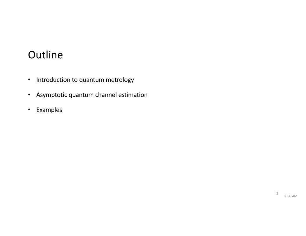
Outline
• Introduction to quantum metrology
• Asymptotic quantum channel estimation
• Examples
9:56 AM2
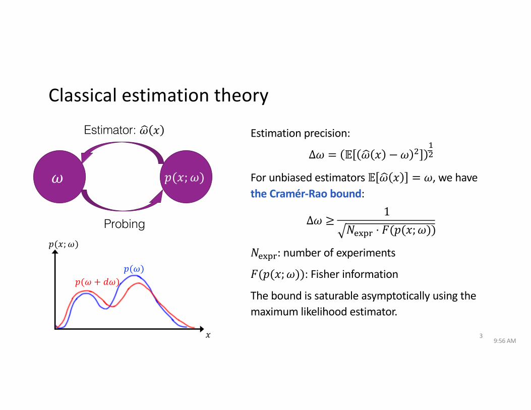
Classical estimation theory
Estimation precision:
Δ𝜔 = 𝔼 %𝜔 𝑥 −𝜔 !"!
For unbiased estimators 𝔼 %𝜔 𝑥 = 𝜔, we have the Cramér-Rao bound:
Δ𝜔 ≥1
𝑁#$%& ⋅ 𝐹(𝑝(𝑥;𝜔))
𝑁#$%&: number of experiments
𝐹(𝑝(𝑥;𝜔)): Fisher information
The bound is saturable asymptotically using the maximum likelihood estimator.
𝜔
Probing
𝑝(𝑥; 𝜔)
Estimator: %𝜔 𝑥
𝑝(𝜔)𝑝(𝜔 + 𝑑𝜔)
𝑥
𝑝(𝑥; 𝜔)
9:56 AM3
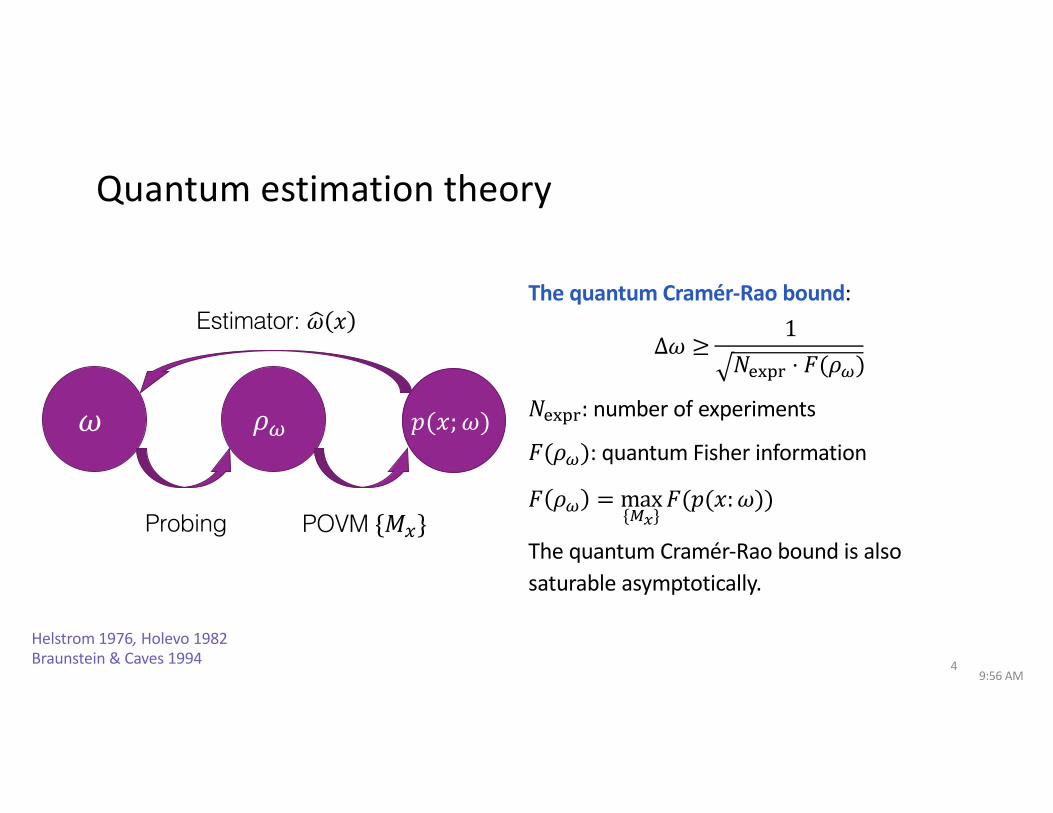
Quantum estimation theory
The quantum Cramér-Rao bound:
Δ𝜔 ≥1
𝑁#$%& ⋅ 𝐹(𝜌')
𝑁#$%&: number of experiments
𝐹(𝜌'): quantum Fisher information
𝐹 𝜌' = max{)!}
𝐹(𝑝(𝑥:𝜔))
The quantum Cramér-Rao bound is also saturable asymptotically.
𝜔 𝜌!
Probing
𝑝(𝑥; 𝜔)
POVM {𝑀)}
Estimator: %𝜔 𝑥
Helstrom 1976, Holevo 1982Braunstein & Caves 1994
9:56 AM4
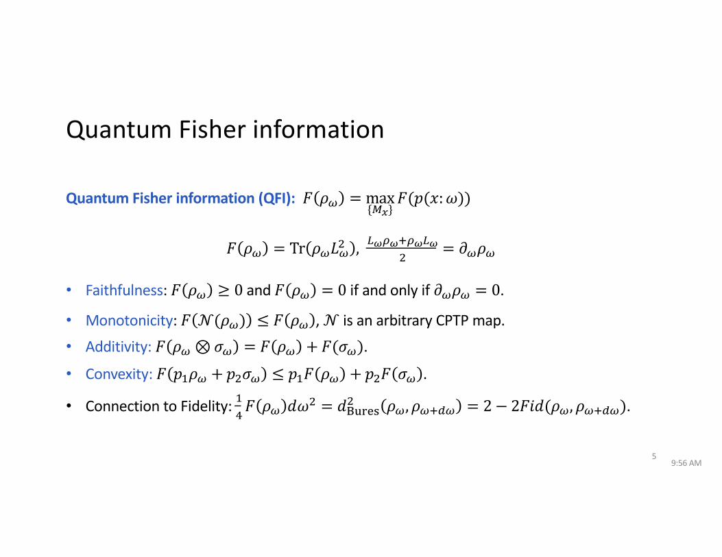
Quantum Fisher information
Quantum Fisher information (QFI): 𝐹 𝜌' = max{)!}
𝐹(𝑝(𝑥:𝜔))
𝐹 𝜌' = Tr 𝜌'𝐿'! , +","-,"+"! = 𝜕'𝜌'
• Faithfulness: 𝐹 𝜌' ≥ 0 and 𝐹 𝜌' = 0 if and only if 𝜕'𝜌' = 0.
• Monotonicity: 𝐹 𝒩(𝜌') ≤ 𝐹 𝜌' , 𝒩 is an arbitrary CPTP map.
• Additivity: 𝐹 𝜌'⊗𝜎' = 𝐹 𝜌' +𝐹(𝜎'). • Convexity: 𝐹 𝑝"𝜌' +𝑝!𝜎' ≤ 𝑝"𝐹 𝜌' +𝑝!𝐹 𝜎' .
• Connection to Fidelity: ".𝐹 𝜌' 𝑑𝜔! = 𝑑/0! 𝜌', 𝜌'-2' = 2− 2𝐹𝑖𝑑(𝜌', 𝜌'-2').
9:56 AM5
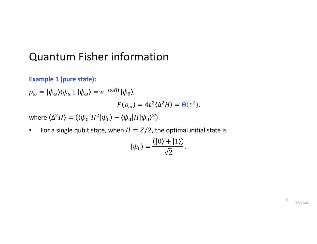
Quantum Fisher information
Example 1 (pure state):
𝜌' = |𝜓'⟩⟨𝜓'|, 𝜓' = 𝑒34'56 𝜓7 ,
𝐹 𝜌' = 4𝑡! Δ!𝐻 = Θ 𝑡! ,
where Δ!𝐻 = 𝜓7 𝐻! 𝜓7 − 𝜓7 𝐻 𝜓7 ! .
• For a single qubit state, when 𝐻 = 𝑍/2, the optimal initial state is
𝜓7 =0 + 1
2.
9:56 AM6
9:56 AM7
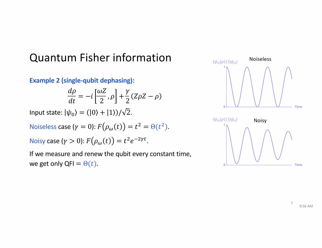
Quantum Fisher information
Example 2 (single-qubit dephasing):𝑑𝜌𝑑𝑡 = −𝑖
𝜔𝑍2 , 𝜌 +
𝛾2 𝑍𝜌𝑍 − 𝜌
Input state: 𝜓7 = 0 + 1 / 2.
Noiseless case (𝛾 = 0): 𝐹 𝜌' 𝑡 = 𝑡! = Θ(𝑡!).
Noisy case (𝛾 > 0): 𝐹 𝜌' 𝑡 = 𝑡!𝑒3!86.
If we measure and renew the qubit every constant time, we get only QFI= Θ(𝑡).
Noiseless𝜓! 𝜌 𝑡 |𝜓!⟩
Noisy𝜓! 𝜌 𝑡 |𝜓!⟩
Quantum Fisher information
9:56 AM8
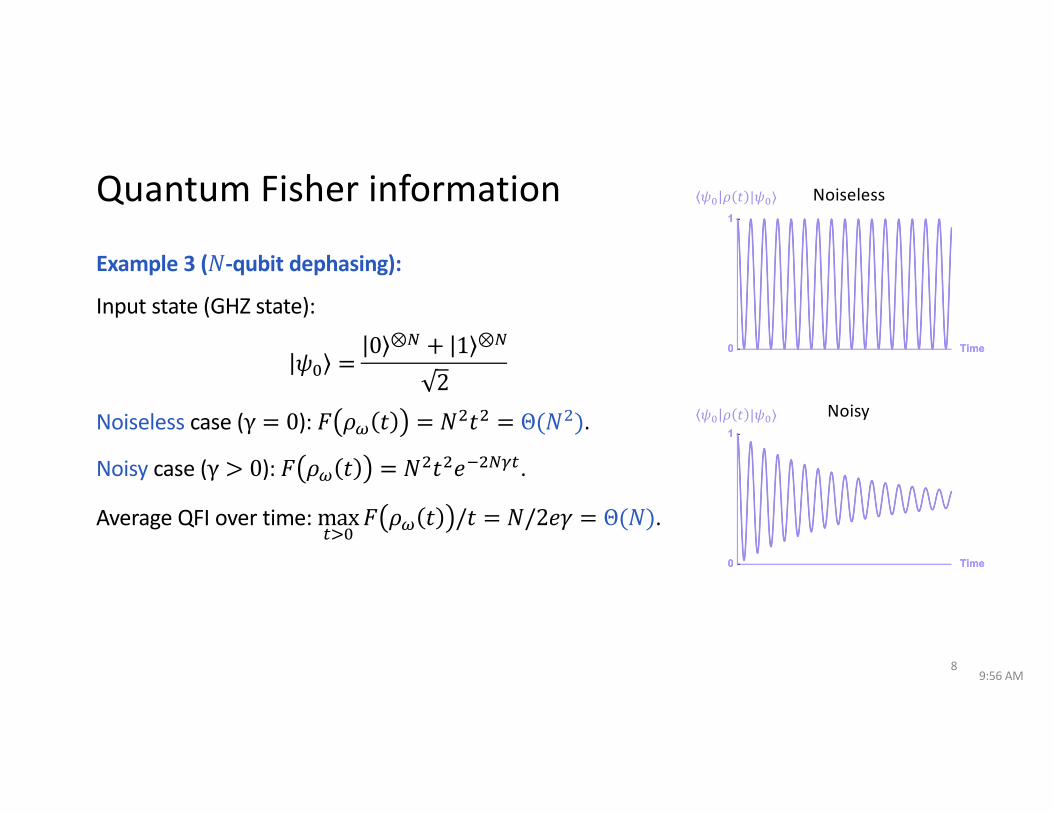
Example 3 (𝑁-qubit dephasing):
Input state (GHZ state):
𝜓7 =0 ⊗: + 1 ⊗:
2Noiseless case (γ = 0): 𝐹 𝜌' 𝑡 = 𝑁!𝑡! = Θ(𝑁!).
Noisy case (γ > 0): 𝐹 𝜌' 𝑡 = 𝑁!𝑡!𝑒3!:86.
Average QFI over time: max6;7
𝐹 𝜌' 𝑡 /𝑡 = 𝑁/2𝑒𝛾 = Θ(𝑁).
Noiseless𝜓! 𝜌 𝑡 |𝜓!⟩
Noisy𝜓! 𝜌 𝑡 |𝜓!⟩
Quantum Fisher information
In quantum metrology, the resource we care about is the number of channels used𝑁 or the probing time 𝑡. There are two types of estimation precision limits:
• The Heisenberg limit (HL): QFI = Θ(𝑁!) or Θ(𝑡!)
— the ultimate estimation precision limit allowed by quantum mechanics.
• The standard quantum limit (SQL): QFI = Θ(𝑁) or Θ(𝑡)
— achievable using “classical” strategies (no need to maintain the coherence in & between probes for a long time).
9:56 AM9
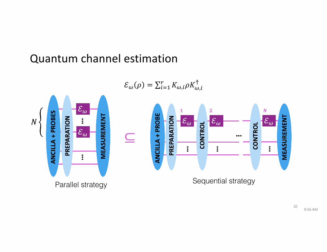
Quantum channel estimation
ℰ* 𝜌 = ∑+,-. 𝐾*,+𝜌𝐾*,+0
9:56 AM
Sequential strategy
⊆
10
Parallel strategy
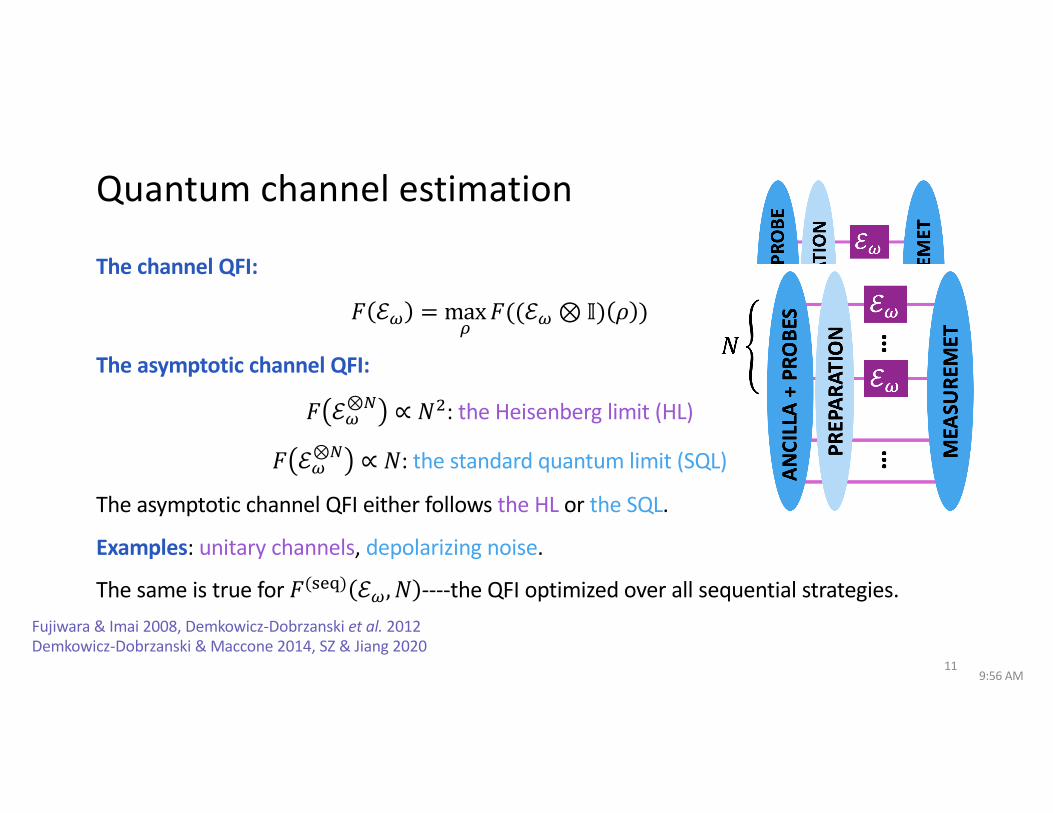
Quantum channel estimation
The channel QFI:
𝐹 ℰ' = max,𝐹((ℰ'⊗𝕀) 𝜌 )
The asymptotic channel QFI:
𝐹 ℰ'⊗: ∝ 𝑁!: the Heisenberg limit (HL)
𝐹 ℰ'⊗: ∝ 𝑁: the standard quantum limit (SQL)
The asymptotic channel QFI either follows the HL or the SQL.
Examples: unitary channels, depolarizing noise.
The same is true for 𝐹(1#=) ℰ', 𝑁 ----the QFI optimized over all sequential strategies.
9:56 AM11
Fujiwara & Imai 2008, Demkowicz-Dobrzanski et al. 2012Demkowicz-Dobrzanski & Maccone 2014, SZ & Jiang 2020
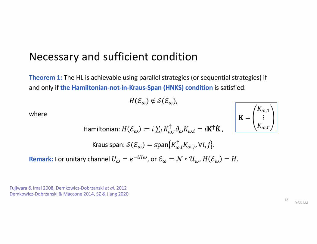
Necessary and sufficient condition
Theorem 1: The HL is achievable using parallel strategies (or sequential strategies) if and only if the Hamiltonian-not-in-Kraus-Span (HNKS) condition is satisfied:
𝐻(ℰ') ∉ 𝒮(ℰ'),
where
Hamiltonian: 𝐻 ℰ' ≔ 𝑖∑4𝐾',4@ 𝜕'𝐾',4 = 𝑖𝐊@�̇� ,
Kraus span: 𝒮(ℰ') = span 𝐾',4@ 𝐾',A, ∀𝑖, 𝑗 .
Remark: For unitary channel 𝑈' = 𝑒345', or ℰ' =𝒩 ∘𝒰', 𝐻 ℰ' = 𝐻.
9:56 AM12
Fujiwara & Imai 2008, Demkowicz-Dobrzanski et al. 2012Demkowicz-Dobrzanski & Maccone 2014, SZ & Jiang 2020
𝐊 =𝐾',"⋮
𝐾',B
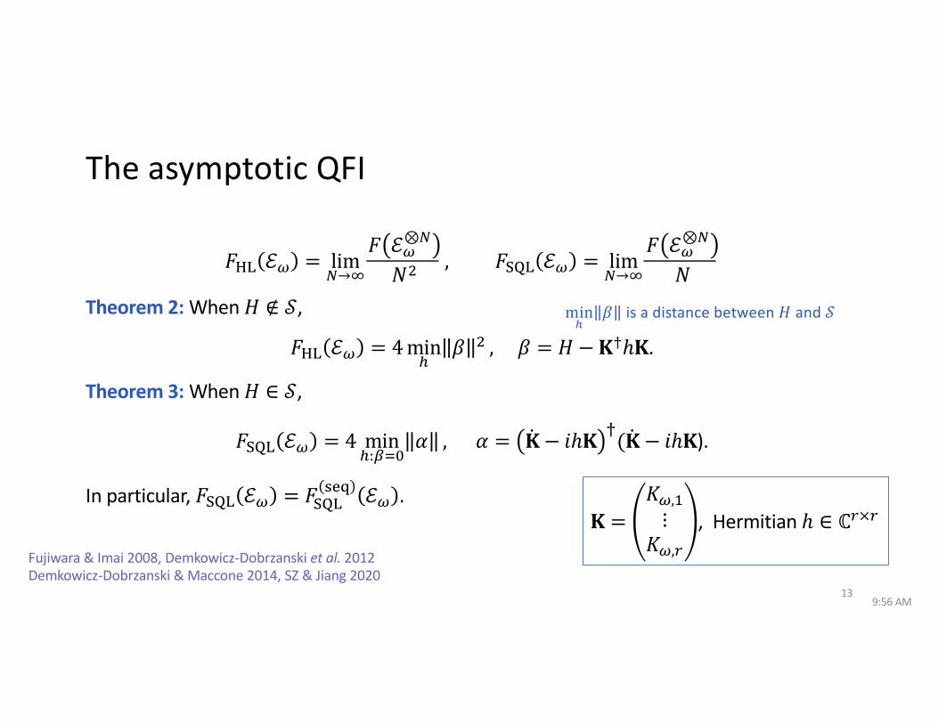
The asymptotic QFI
𝐹CD ℰ' = lim:→F
𝐹 ℰ'⊗:
𝑁! , 𝐹GHD ℰ' = lim:→F
𝐹 ℰ'⊗:
𝑁Theorem 2: When 𝐻 ∉ 𝒮,
𝐹CD ℰ' = 4minI
𝛽 ! , 𝛽 = 𝐻 −𝐊!ℎ𝐊.
Theorem 3: When 𝐻 ∈ 𝒮,
𝐹GHD ℰ' = 4 minI:KL7
𝛼 , 𝛼 = �̇� − 𝑖ℎ𝐊 0(�̇� − 𝑖ℎ𝐊).
In particular, 𝐹GHD ℰ' = 𝐹GHD1#= ℰ' .
9:56 AM13
𝐊 =𝐾',"⋮
𝐾',B, Hermitian ℎ ∈ ℂB×B
Fujiwara & Imai 2008, Demkowicz-Dobrzanski et al. 2012Demkowicz-Dobrzanski & Maccone 2014, SZ & Jiang 2020
min!
𝛽 is a distance between 𝐻 and 𝒮
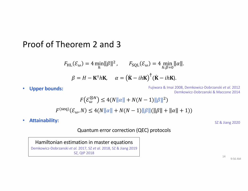
Proof of Theorem 2 and 3
𝐹CD ℰ' = 4minI
𝛽 ! , 𝐹GHD ℰ' = 4 minI:KL7
𝛼 .
𝛽 = 𝐻 −𝐊!ℎ𝐊, 𝛼 = �̇� − 𝑖ℎ𝐊 0(�̇� − 𝑖ℎ𝐊).
• Upper bounds:
𝐹 ℰ'⊗: ≤ 4(𝑁 𝛼 +𝑁(𝑁 − 1)‖𝛽‖!)
𝐹(1#=) ℰ', 𝑁 ≤ 4(𝑁 𝛼 +𝑁(𝑁 − 1) 𝛽 ( 𝛽 + 𝛼 + 1))
• Attainability:
Quantum error correction (QEC) protocols
9:56 AM14
Fujiwara & Imai 2008, Demkowicz-Dobrzanski et al. 2012 Demkowicz-Dobrzanski & Maccone 2014
SZ & Jiang 2020
Hamiltonian estimation in master equationsDemkowicz-Dobrzanski et al. 2017, SZ et al. 2018, SZ & Jiang 2019
SZ, QIP 2018
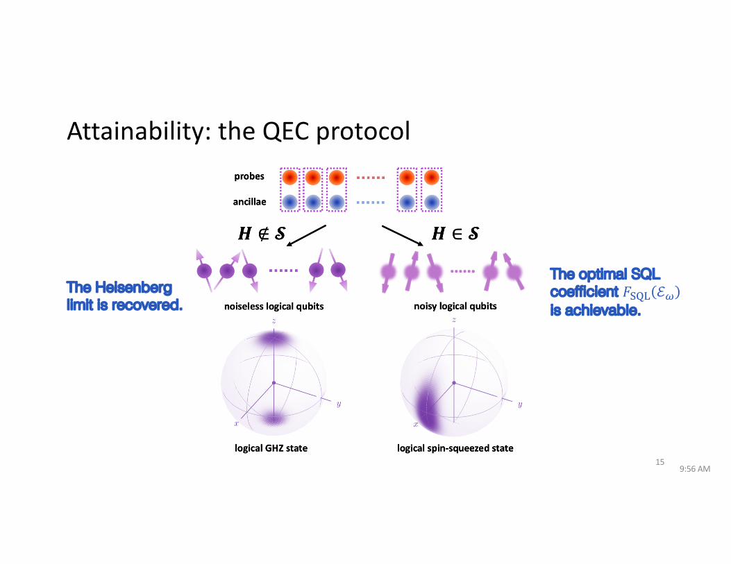
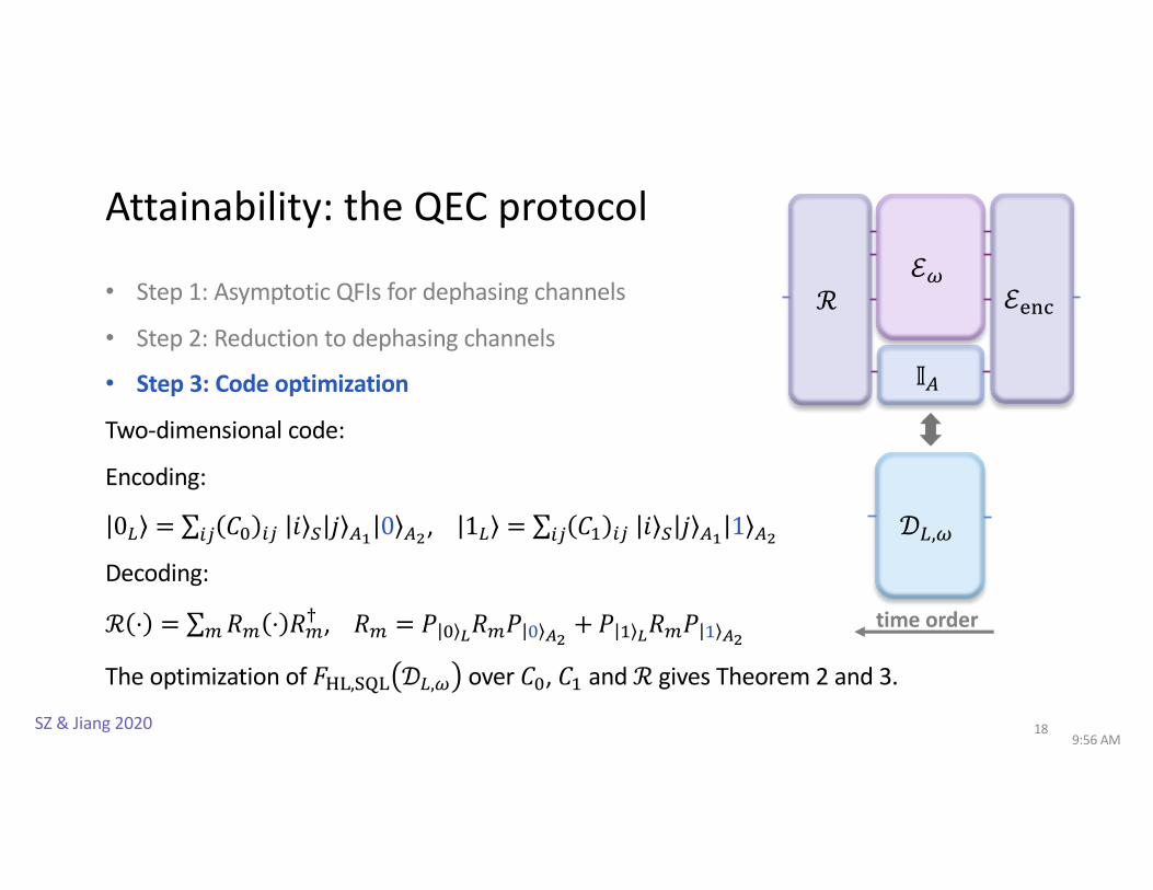
Attainability: the QEC protocol
9:56 AM15
The Heisenberg limit is recovered.
The optimal SQL coefficient 𝐹"#$ ℰ%is achievable.
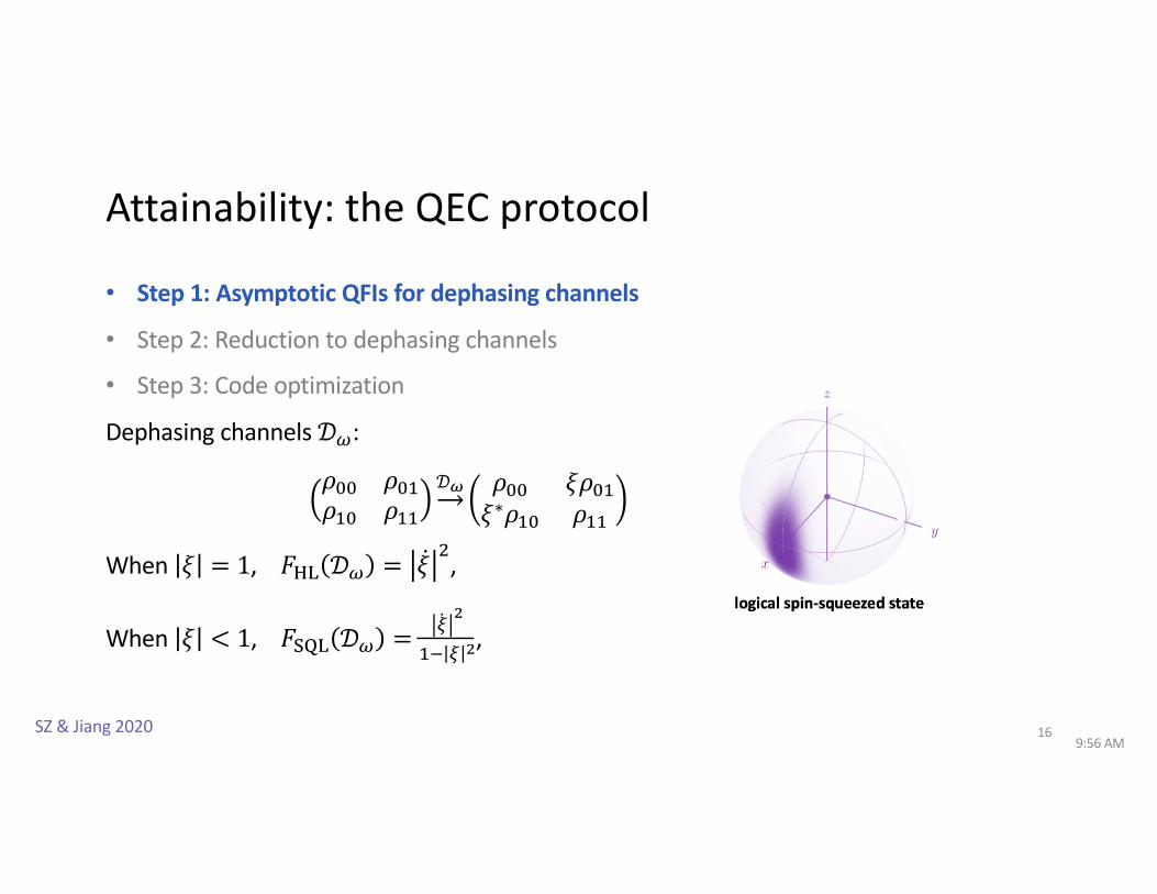
Attainability: the QEC protocol
• Step 1: Asymptotic QFIs for dephasing channels
• Step 2: Reduction to dephasing channels
• Step 3: Code optimization
Dephasing channels𝒟':
𝜌77 𝜌7"𝜌"7 𝜌""
𝒟" 𝜌77 𝜉𝜌7"𝜉∗𝜌"7 𝜌""
When 𝜉 = 1, 𝐹CD 𝒟' = �̇� !,
When 𝜉 < 1, 𝐹GHD 𝒟' = Q̇(
"3 Q (,
9:56 AM16SZ & Jiang 2020
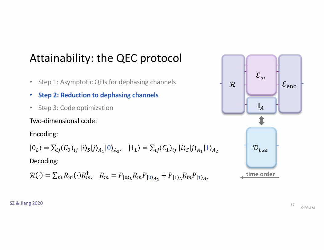
Attainability: the QEC protocol
• Step 1: Asymptotic QFIs for dephasing channels
• Step 2: Reduction to dephasing channels
• Step 3: Code optimization
Two-dimensional code:
Encoding:
0+ = ∑4A 𝐶7 4A 𝑖 R 𝑗 S) 0 S(, 1+ = ∑4A 𝐶" 4A 𝑖 R 𝑗 S) 1 S(
Decoding:
ℛ ⋅ = ∑T𝑅T ⋅ 𝑅T! , 𝑅T = 𝑃 7 *𝑅T𝑃 7 +(
+𝑃 " *𝑅T𝑃 " +(
9:56 AM17
𝒟7,*
time order
ℰ*
𝕀8
ℛ ℰ9:;
SZ & Jiang 2020
Attainability: the QEC protocol
• Step 1: Asymptotic QFIs for dephasing channels
• Step 2: Reduction to dephasing channels
• Step 3: Code optimization
Two-dimensional code:
Encoding:
0+ = ∑4A 𝐶7 4A 𝑖 R 𝑗 S) 0 S(, 1+ = ∑4A 𝐶" 4A 𝑖 R 𝑗 S) 1 S(
Decoding:
ℛ ⋅ = ∑T𝑅T ⋅ 𝑅T! , 𝑅T = 𝑃 7 *𝑅T𝑃 7 +(
+𝑃 " *𝑅T𝑃 " +(
The optimization of 𝐹CD,GHD 𝒟+,' over 𝐶7, 𝐶" and ℛ gives Theorem 2 and 3.
9:56 AM18SZ & Jiang 2020
𝒟7,*
time order
ℰ*
𝕀8
ℛ ℰ9:;
Example 1: Pauli 𝑍 signal with bit-flip noise
ℰ' 𝜌 = 𝒩 ∘𝒰' 𝜌 ,
𝒩 𝜌 = 1− 𝑝 𝜌 + 𝑝𝑋𝜌𝑋, 𝑈' = 𝑒3,"-( ,
𝐻 = 𝑍 ∉ 𝒮 = span{𝐼, 𝑋}
Optimal code: 0+ = 0 R⊗ 0 S , 1+ = 1 R⊗ 1 S.
After error:
(𝑋⊗ 𝐼) 0+ = 1 R⊗ 0 S , (𝑋⊗ 𝐼) 1+ = 0 R⊗ 1 S.
Recovery:
Measure 𝑆 = 𝑍⊗𝑍. If 𝑆 = −1, flip the probe with 𝑋; otherwise do nothing.
199:56 AM
Kessler et al. 2014, Arrad et al. 2014, Dur et al. 2014, Unden et al. 2016
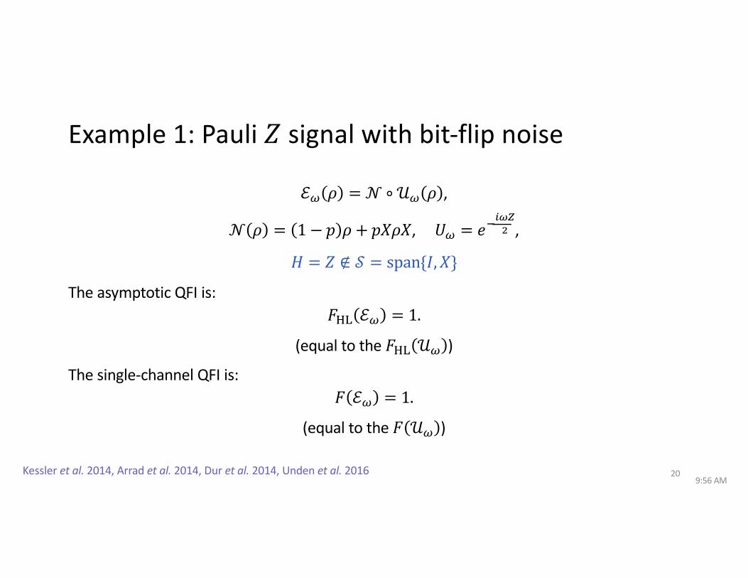
Example 1: Pauli 𝑍 signal with bit-flip noise
ℰ' 𝜌 = 𝒩 ∘𝒰' 𝜌 ,
𝒩 𝜌 = 1− 𝑝 𝜌 + 𝑝𝑋𝜌𝑋, 𝑈' = 𝑒3,"-( ,
𝐻 = 𝑍 ∉ 𝒮 = span{𝐼, 𝑋}
The asymptotic QFI is: 𝐹CD ℰ' = 1.
(equal to the 𝐹CD 𝒰' )
The single-channel QFI is: 𝐹 ℰ' = 1.
(equal to the 𝐹 𝒰' )
209:56 AM
Kessler et al. 2014, Arrad et al. 2014, Dur et al. 2014, Unden et al. 2016
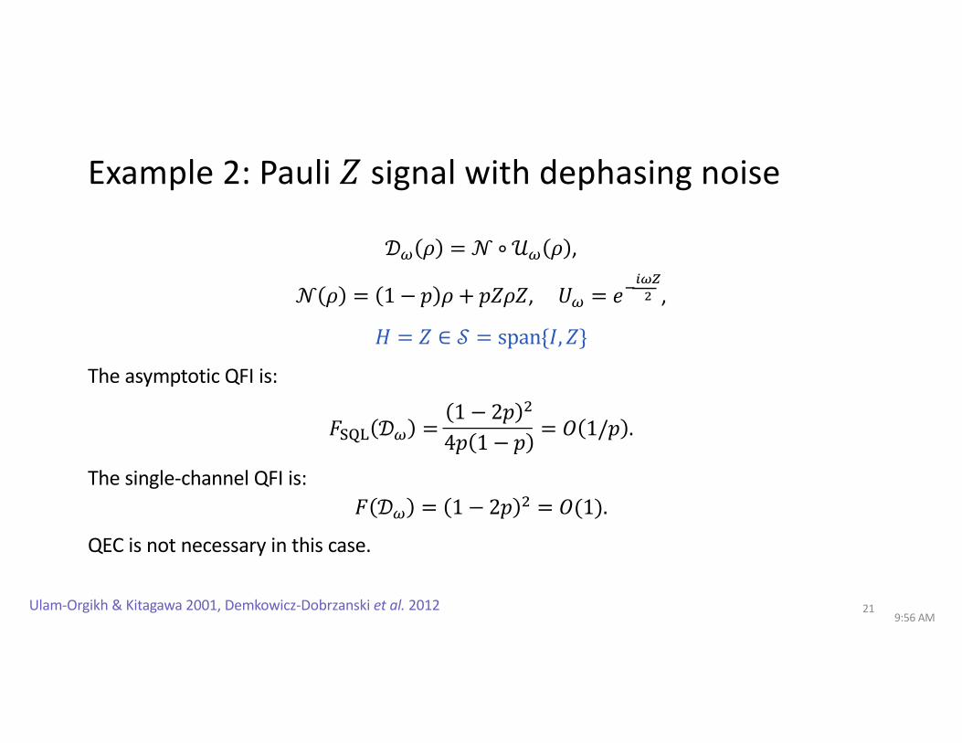
Example 2: Pauli 𝑍 signal with dephasing noise
𝒟' 𝜌 = 𝒩 ∘𝒰' 𝜌 ,
𝒩 𝜌 = 1− 𝑝 𝜌 + 𝑝𝑍𝜌𝑍, 𝑈' = 𝑒3,"-( ,
𝐻 = 𝑍 ∈ 𝒮 = span{𝐼, 𝑍}
The asymptotic QFI is:
𝐹GHD 𝒟' =1− 2𝑝 !
4𝑝 1 − 𝑝 = 𝑂 1/𝑝 .
The single-channel QFI is: 𝐹 𝒟' = 1− 2𝑝 ! = 𝑂(1).
QEC is not necessary in this case.
21Ulam-Orgikh & Kitagawa 2001, Demkowicz-Dobrzanski et al. 20129:56 AM
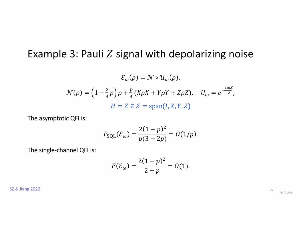
Example 3: Pauli 𝑍 signal with depolarizing noise
ℰ' 𝜌 = 𝒩 ∘𝒰' 𝜌 ,
𝒩 𝜌 = 1− U.𝑝 𝜌 + V
.(𝑋𝜌𝑋 + 𝑌𝜌𝑌 + 𝑍𝜌𝑍), 𝑈' = 𝑒3
,"-( ,
𝐻 = 𝑍 ∈ 𝒮 = span{𝐼, 𝑋, 𝑌, 𝑍}
The asymptotic QFI is:
𝐹GHD ℰ' =2 1− 𝑝 !
𝑝(3 − 2𝑝) = 𝑂 1/𝑝 .
The single-channel QFI is:
𝐹 ℰ' =2 1− 𝑝 !
2 − 𝑝 = 𝑂(1).
229:56 AM
SZ & Jiang 2020
Conclusions and outlook
• The structure of the noise and the Hamiltonian determines the estimation precision limit in quantum metrology.
• Quantum error correction is powerful – recovering the HL, achieving the optimal SQL.
• Future directions: • parallel strategies vs sequential strategies when the HL is achievable
• multi-parameter estimation for general quantum channels
• fault-tolerant QEC for quantum metrology
239:56 AM
Thank you! Liang Jiang