arX

iv:c

ond-

mat

/951

2099

v1 1

2 D

ec 1

995

Conformal Field Theory Approach to the Kondo Effect∗

Ian Affleck

Canadian Institute for Advanced Research and Physics Department, University of British Columbia, Vancouver, BC,

V6T 1Z1, Canada

Recently, a new approach, based on boundary conformal field theory, has been applied to a varietyof quantum impurity problems in condensed matter and particle physics. A particularly enlighteningexample is the multi-channel Kondo problem. In this review some earlier approaches to the Kondoproblem are discussed, the needed material on boundary conformal field theory is developed andthen this new method is applied to the multi-channel Kondo problem.

OUTLINE

I. Renormalization Group and Fermi Liquid Approaches to the Kondo EffectA) Introduction to The Kondo EffectB) Renormalization Group ApproachC) Mapping to a One Dimensional ModelD) Fermi Liquid Approach at Low T

II. Conformal Field Theory (“Luttinger Liquid”) Techniques: Separation of Charge and Spin De-grees of Freedom, Current Algebra, “Gluing Conditions”, Finite-Size Spectrum

III. Conformal Field Theory Approach to the Kondo Effect: “Completing the Square”A) Leading Irrelevant Operator, Specific Heat, Susceptibility, Wilson Ratio, Resistivity at T > 0

IV. Introduction to the Multi-Channel Kondo Effect: Underscreening and OverscreeningA) Large-k LimitB) Current Algebra Approach

V. Boundary Conformal Field Theory

VI. Boundary Conformal Field Theory Results on the Multi-Channel Kondo Effect:A) Fusion and the Finite-Size SpectrumB) Impurity EntropyC) Boundary Green’s Functions: Two-Point Functions, T=0 ResistivityD) Four-Point Boundary Green’s Functions, Spin-Density Green’s FunctionE) Boundary Operator Content and Leading Irrelevant Operator:Specific Heat, Susceptibility, Wilson Ratio, Resistivity at T > 0

1

I. RENORMALIZATION GROUP AND FERMI LIQUID APPROACHES TO THE KONDO EFFECT

A. Introduction to the Kondo Effect

Most mechanisms contributing to the resistivity of metals, ρ(T ), give either ρ(T ) decreasing to 0,as T → 0 (phonons or electron-electron interactions), or ρ(T ) → constant, as T → 0 (non-magnetricimpurities). However, metals containing magnetic impurities show a ρ(T ) which increases as T → 0.This was explained by Kondo1 in 1964 using a simple Hamiltonian:

H =∑

~kα

ψ†α~kψ~kαǫ(k) + λ~S ·

∑

~k ~k′

ψ†~k

~σ

2ψ~k′ (1.1)

where ψ~kα’s are conduction electron annihilation operators, (of momentum ~k, spin α) and ~S repre-sents the spin of the magnetic impurity with

[Sa, Sb] = iǫabcSc.

The interaction term represents an impurity spin interacting with the electron spin at ~x = 0.With the above Hamiltonian, the Born approximation gives: ρ(T ) ∼ λ2, independent of T . The

next order term has a divergent coefficient at T = 0:

ρ(T ) ∼ [λ+ νλ2 lnD

T+ ...]2 (1.2)

Here D is the band-width, ν the density of states. This result stimulated an enormous amount oftheoretical work. As Nozieres put it, “Theorists ‘diverged’ on their own, leaving the experiment

realities way behind”.2 What happens at low T , i.e. T ∼ TK = De−1

υλ ? In that case the O(λ2)term will be as big as the term of O(λ). What about the O(λ3) term? Such questions helped leadto the development of the renormalization group needed to understand the problem.

In particle physics such a growth of a coupling constant at low energies explains quark con-finement (1973) and “asymptotic freedom” at E → ∞. To solve these problems, Wilson3 de-veloped a very powerful numerical renormalization group approach. The Kondo model was also“solved” by the Bethe ansatz4,5 which gives the specific heat and magnetization. Nozieres,2,7

following ideas of Anderson6 and Wilson,3 developed a very simple, and in a sense exact, pic-ture of the low T behaviour. With A. Ludwig, I have generalized and reformulated Nozieres’approach9,10,11,12,13,14,15,16 using recent results in conformal field theory. The latter approachis very general and can be applied to a number of other problems including multi-channeland higher spin Kondo effect,9,10,11,12,13,14,15,16 two (or more)-impurity Kondo effects,17,18 im-purity assisted tunneling,19 impurities in one-dimensional conductors (“quantum wires”)20 or 1Dantiferromagnets,21,22 baryon-monopole interaction,23. Some of these problems, including themulti-channel Kondo effect, exhibit non-Fermi liquid behaviour. These are among the very fewexactly solved problems that do this (the others are 1D Luttinger liquids). It has been sug-gested that this may be connected with exotic behaviour of certain compounds, including high-Tc

superconductors.24,25

B. Renormalization Group

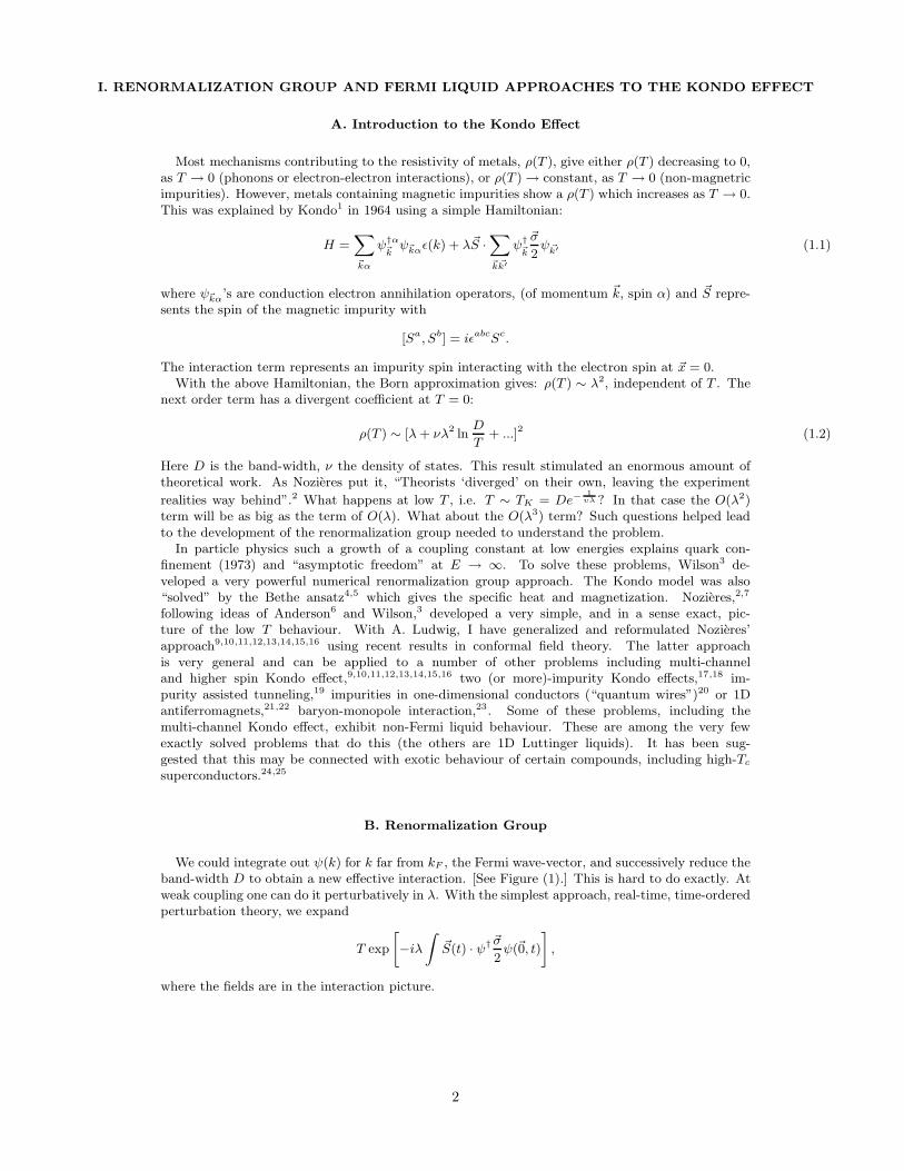
We could integrate out ψ(k) for k far from kF , the Fermi wave-vector, and successively reduce theband-width D to obtain a new effective interaction. [See Figure (1).] This is hard to do exactly. Atweak coupling one can do it perturbatively in λ. With the simplest approach, real-time, time-orderedperturbation theory, we expand

T exp

[

−iλ∫

~S(t) · ψ†~σ

2ψ(~0, t)

]

,

where the fields are in the interaction picture.

2

EF

kF

2D’

E

k

2DFIG. 1. Reduction of the cut-off from D to D′.

As ~S(t) is independent of t, we simply multiply powers of ~S using

[Sa, Sb] = iǫabcSc, ~S2 = s(s+ 1).

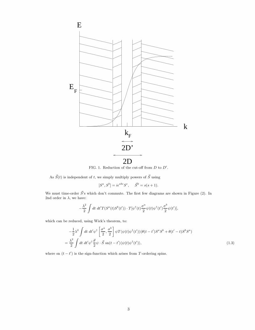
We must time-order ~S’s which don’t commute. The first few diagrams are shown in Figure (2). In2nd order in λ, we have:

−λ2

2

∫

dt dt′T (Sa(t)Sb(t′)) · T [ψ†(t)σa

2ψ(t)ψ†(t′)

σb

2ψ(t′)],

which can be reduced, using Wick’s theorem, to:

−1

2λ2

∫

dt dt′ψ†[

σa

2,σb

2

]

ψT 〈ψ(t)ψ†(t′)〉(θ(t− t′)SaSb + θ(t′ − t)SbSa)

=λ2

2

∫

dt dt′ψ† ~σ

2ψ · ~S sn(t− t′)〈ψ(t)ψ†(t′)〉, (1.3)

where sn (t− t′) is the sign-function which arises from T -ordering spins.

3

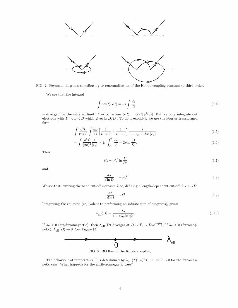
FIG. 2. Feynman diagrams contributing to renormalization of the Kondo coupling constant to third order.

We see that the integral∫

dtǫ(t)G(t) = −i∫

dt

|t| (1.4)

is divergent in the infrared limit: t → ∞, where G(t) = 〈ψ(t)ψ†(0)〉. But we only integrate outelectrons with D′ < k < D which gives lnD/D′. To do it explicitly we use the Fourier transformedform:

∫

d3k

(2π)3

∫

dω

2π

[

1

iω + δ+

1

iω − δ

]

i

ω − ǫk + iδsn(ǫk)(1.5)

=

∫

d3~k

(2π)31

|ǫk|≈ 2ν

∫ D

D′

dǫ

ǫ= 2ν ln

D

D′ . (1.6)

Thus

δλ = νλ2 lnD

D′ , (1.7)

and

dλ

d lnD= −νλ2. (1.8)

We see that lowering the band cut-off increases λ or, defining a length-dependent cut-off, l ∼ vF /D,

dλ

d ln l= νλ2. (1.9)

Integrating the equation (equivalent to performing an infinite sum of diagrams), gives:

λeff(D) =λ0

1 − νλ0 ln D0D

. (1.10)

If λ0 > 0 (antiferromagnetic), then λeff(D) diverges at D ∼ Tk ∼ D0e− 1

νλ0 , If λ0 < 0 (ferromag-netic), λeff(D) → 0. See Figure (3).

eff0λ

FIG. 3. RG flow of the Kondo coupling.

The behaviour at temperature T is determined by λeff(T ): ρ(T ) → 0 as T → 0 for the ferromag-netic case. What happens for the antiferromagnetic case?

4

C. Mapping to a One-Dimensional Model

The above discussion can be simplified if we map the model into a one dimensional one. Weassume a spherically symmetric ǫ(~k),

ǫ(k) =k2

2m− ǫF ≈ vF (k − kF ), (1.11)

and a δ−function Kondo interaction. There is only s-wave scattering, i.e.

ψ(~k) =1√4πk

ψ0(k) + higher harmonics,

H0 =

∫

dkψ†0kψ0kǫ(k) + higher harmonics,

HINT = λvF ν

∫

dkdk′ψ†0,k

~σ

2ψ0,k′ · ~S, (1.12)

where ν = k2F /2π

2vF is the density of states per spin. This can also be written in terms of radialco-ordinate. We eliminate all modes except for a band width 2D: |k − kF | < D. Defining left andright movers (incoming and outgoing waves),

ΨL,R(r) ≡∫ ∧

−∧dke±ikr ψ0(k + kF ), ⇒ ψL(0) = ψR(0), (1.13)

we have

H0 =vF

2π

∫ ∞

0

dr(ψ†Lid

drψL − ψ†

Rid

drψR) (note the unconventional normalization),

HINT = vFλψL(0)†~σ

2ψL(0) · ~S. (1.14)

Here we have redefined a dimensionless Kondo coupling, λ→ λν. Using the notation

ψL = ψL(x, τ ) = ψL(z = τ + ix), ψR(x, τ ) = ψR(z∗ = τ − ix), (1.15)

where τ is imaginary time and x = r, (and we set vF = 1) we have

〈ψL(z)ψ+L (0)〉 =

1

z, 〈ψR(z∗)ψ†

R(0)〉 =1

z∗. (1.16)

Alternatively, since

ψL(0, τ ) = ψR(0, τ ) ψL = ψL(z), ψR = ψR(z∗), (1.17)

we may consider ψR to be the continuation of ψL to the negative r-axis:

ψR(x, τ ) ≡ ψL(−x, τ ). (1.18)

Now we obtain a relativistic (1+1) dimensional field theory ( a “chiral” one, containing left-moversonly) interacting with the impurity at x = 0 with

H0 =vF

2π

∫ ∞

−∞dxψ†

Lid

dxψL (1.19)

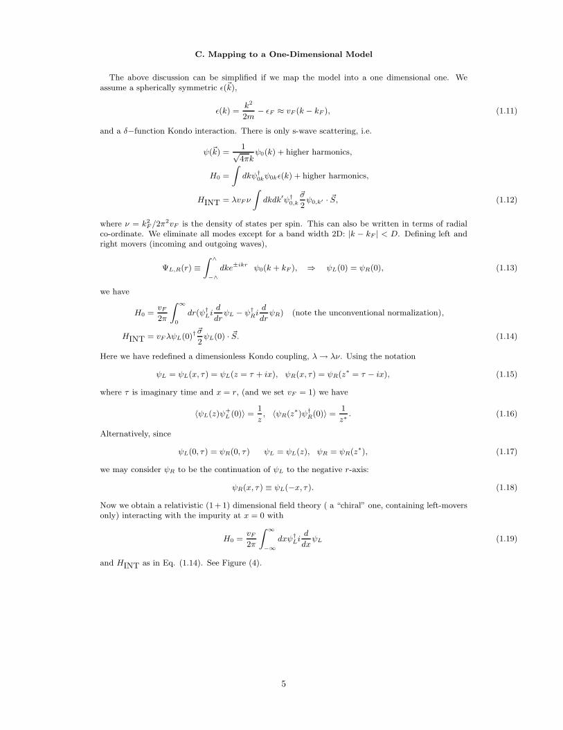
and HINT as in Eq. (1.14). See Figure (4).

5

LL

L

R

FIG. 4. Reflecting the left-movers to the negative axis.

D. Fermi Liquid Approach at Low T

What is the T → 0 behavior of the antiferromagetic Kondo model? The simplest assumption isλeff → ∞. But what does that really mean? Consider the strong coupling limit of a lattice model,2

for convenience, in spatial dimension D = 1. (D doesn’t really matter since we can always reducethe model to D = 1.)

H = t∑

i

(ψ†iψi+1 + ψ†

i+1ψi) + λ~S · ψ†0

~σ

2ψ0 (1.20)

Consider the limit λ >> |t|. The groundstate of the interaction term will be the following con-figuration: one electron at the site 0 forms a singlet with the impurity: | ⇑↓〉 − | ⇓↑〉. (We as-sume SIMP = 1/2). Now we do perturbation theory in t. We have the following low energy states:an arbitary electron configuration occurs on all other sites-but other electrons or holes are forbiddento enter the site-0, since that would destroy the singlet state, costing an energy, ∆E ∼ λ >> t.Thus we simply form free electron Bloch states with the boundary condition φ(0) = 0, where φ(i) isthe single-electron wave-function. Note that at zero Kondo coupling, the parity even single particlewave-functions are of the form φ(i) = cos ki and the parity odd ones are of the form φ(i) = sin ki.On the other hand, at λ → ∞ the parity even wave-functions become φ(i) = | sin ki|, while theparity odd ones are unaffected.

The behaviour of the parity even channel corresponds to a π/2 phase shift in the s-wave channel.

φj ∼ e−ik|j| + e+2iδeik|j|, δ = π/2. (1.21)

In terms of left and right movers on r > 0 we have changed the boundary condition,

ψL(0) = ψR(0), λ = 0,

ψL(0) = −ψR(0), λ = ∞. (1.22)

The strong coupling fixed point is the same as the weak coupling fixed point except for a changein boundary conditions (and the removal of the impurity). In terms of the left-moving descriptionof the P -even sector, the phase of the left-mover is shifted by π as it passes the origin. Imposinganother boundary condition a distance l away quantizes k:

ψ(l) = ψL(l) + ψR(l) = ψL(l) + ψL(−l) = 0,

λ = 0 : k =π

l(n+ 1/2)

λ = ∞ : k =πn

l(1.23)

6

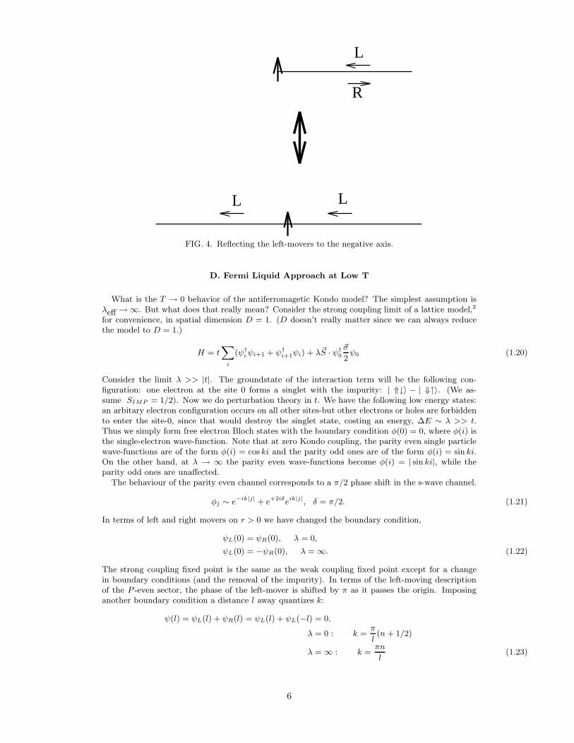
Near the Fermi surface the energies are linearly spaced. Assuming particle-hole symmetry, theFermi energy lies midway between levels or on a level. [See Figures (5) and (6).] The two situationsswitch with the phase shift. Wilson’s numerical RG scheme3 involves calculating the low-lyingspectrum numerically and looking for this shift. This indicates that λ renormalizes to ∞ even if itis initially small. However, now we expect the screening to take place over a longer length scale

ξ ∼ vF

TK∼ vF

De1/νλ. (1.24)

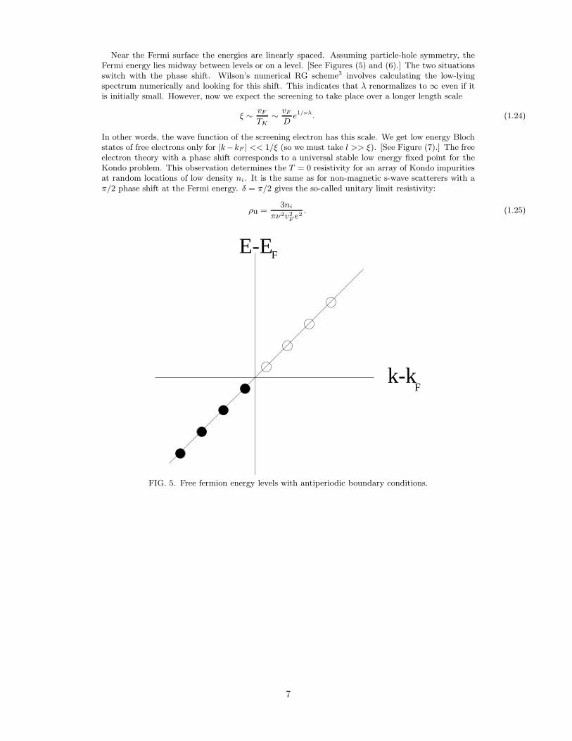
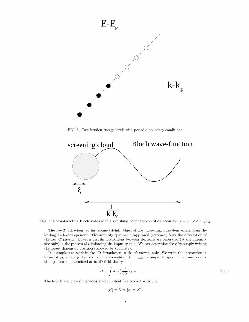
In other words, the wave function of the screening electron has this scale. We get low energy Blochstates of free electrons only for |k−kF | << 1/ξ (so we must take l >> ξ). [See Figure (7).] The freeelectron theory with a phase shift corresponds to a universal stable low energy fixed point for theKondo problem. This observation determines the T = 0 resistivity for an array of Kondo impuritiesat random locations of low density ni. It is the same as for non-magnetic s-wave scatterers with aπ/2 phase shift at the Fermi energy. δ = π/2 gives the so-called unitary limit resistivity:

ρu =3ni

πν2v2F e

2. (1.25)

E-E

F

F

k-k

FIG. 5. Free fermion energy levels with antiperiodic boundary conditions.

7

E-EF

k-kF

FIG. 6. Free fermion energy levels with periodic boundary conditions.

screening cloud

ξ

1k-kF

Bloch wave-function

FIG. 7. Non-interacting Bloch states with a vanishing boundary condition occur for |k − kF | << vF /TK .

The low-T behaviour, so far, seems trivial. Much of the interesting behaviour comes from theleading irrelevant operator. The impurity spin has disappeared (screened) from the description ofthe low -T physics. However certain interactions between electrons are generated (at the impuritysite only) in the process of eliminating the impurity spin. We can determine these by simply writingthe lowest dimension operators allowed by symmetry.

It is simplest to work in the 1D formulation, with left-movers only. We write the interaction interms of ψL, obeying the new boundary condition (but not the impurity spin). The dimension ofthe operator is determined as in 1D field theory

H =

∫

dxψ†Li

d

dxψL + .... (1.26)

The length and time dimensions are equivalent (we convert with vF ),

[H ] = E ⇒ [ψ] = E12 .

8

The interactions are local

δH =∑

i

λiOi(x = 0), [λi] + [Oi] = 1.

So λi has negative energy dimension if [Oi] > 1, implying that it is irrelevant. In RG theory oneusually defines a dimensionless coupling constant by multiplying powers of the cut-off D, if

[λi] = E−a, λi ≡ λiDa,

λi decreases as we lower D:

dλi

dlnD= aλi. (1.27)

Such a coupling, with a > 0, produces no infrared divergences in perturbation theory. The ultravioletones are cancelled by the expicit factors of the ultraviolet cut-off, D, appearing in the Lagrangian,λO/Da. What are the lowest dimension operators allowed by symmetry? Consider ψ+α(0)ψα(0).This has d = 1. However, it is not allowed because it breaks particle-hole symmetry. If particle-holesymmetry is broken then we do get this, a potential scattering term; it adds a term to the phaseshift. Consider another term,

iψ†α d

dxψα(0) − i

d

dxψ†αψα(0). (1.28)

This has d=2 . This term produces a k-dependent phase shift. The only other term with d ≤ 2 isψ†↑ψ↑ψ

†↓ψ↓. This term represents the electron-electron interaction induced by an impurity spin-flip. The first electron flips the impurity spin. This makes it possible for the second electron to flipit back if the electron spin is correct. These are the only d ≤ 2 operators. There are no relevant(d ≤ 1) operators, implying the stability of the low energy fixed point. Note that, by contrast, thehigh energy, zero Kondo coupling, fixed point is unstable. The dimension 1 operator (the Kondointeraction) can occur there because of the presence of the impurity spin.

We can’t calculate these two coupling constants exactly except by using complicated methods:Wilson’s numerical melthod or the Bethe ansatz. They both have dimension E−1. We expect themto be O[1/TK ] by a standard scaling argument. That is, functions of the cut-off D and couplingconstant λ can be replaced by functions of the reduced cut-off, D′ and the renormalized couplingconstant, λeff(D′): f [D, λ] = f [D′, λeff(D′)]. We can lower the cut-off down to TK where λeff isO(1) so f = f(TK , 1) = f(TK). This is a characteristic scale introduced by the infrared divergencesof perturbation theory. For TK << D(λ << 1), Nozieres argued that the two irrelevant couplingconstants have a universal ratio. So there is only one unknown parameter (“the Wilson number”).Essentially all low-temperature information is given by this irrelevant coupling constant, if it wasnot already determined by the π/2 phase shift at kF . I will give a different derivation of the ratioof the two coupling constants later using conformal field theory. We now simply do perturbationtheory in the irrelevant coupling constant ∼ 1/TK . We can determine powers of T by dimensionalanalysis. For the specific heat we find:

C ∼ π

3vFlT + a

T

TK. (1.29)

This is the specific heat for the one-dimensional system with a single impurity at the origin. Notethat the first term is simply the specific heat of the free system, proportional to system length. Thesecond term is independent of length and is the impurity specific heat. It is the result of first orderperturbation theory in the irrelevant coupling constant, of O(1/TK). The (linear) power of T can befixed by dimensional analysis; a is a pure number. Note that while this is formally an “irrelevant”contribution, it in fact gives the leading impurity specific heat at low T . To obtain the specific heatfor the three dimensional system we simply multiply the first term by the ratio νV/(l/2πvF ) i.e. theratio of densities of states per unit energy. For a dilute random array the last term gets multipliedby the number of impurities. At high T we get, approximately, the entropy for a decoupled s=1/2impurity:

S(T ) =πl

3vFT + ln 2. (1.30)

At low T , the impurity entropy decreases to 0:

9

S(T ) =πl

3vFT +

aT

TK. (1.31)

In general we may write:

S(T ) − πl

3vFT ≡ Simp = g(T/TK), (1.32)

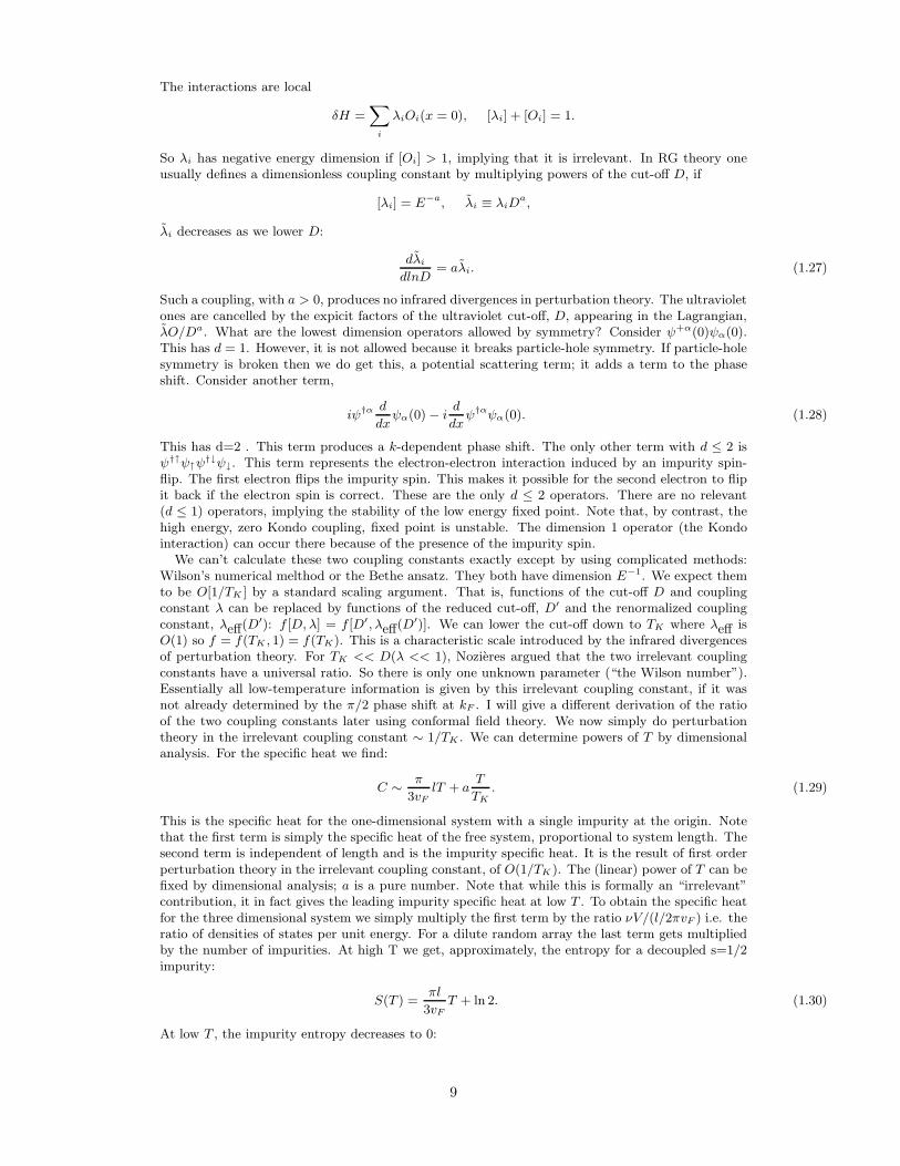
where g is a scaling function which is universal for weak bare coupling. See Figure (8). The behaviourof g(x) for small arguments is determined by RG-improved weak coupling perturbation theory. It’sbehaviour at low T is determined from the theory of the low energy fixed point. Its behaviour atarbitrary T/TK is a property of the universal crossover between fixed points. It has been found fromthe Bethe ansatz.

S

K

TTK

imp

ln 2

aT/T

FIG. 8. Qualitative behaviour of the impurity entropy.

Similarly, the susceptibility, at T = 0, is given by:

χ ∼ l

2πvF+

b

TK. (1.33)

The ratio b/a is universal since the coupling constant (1/TK) drops out. This is known as the WilsonRatio.

At high T , we must (for weak bare coupling) obtain approximately the results for a free spin:

χ ∼ l

2πvF+

1

4T. (1.34)

At lower T , using RG improved perturbation theory this becomes:

χ ∼ l

2πvF+

1

4T

[

1 − 1

ln(T/TK)+ ...

]

. (1.35)

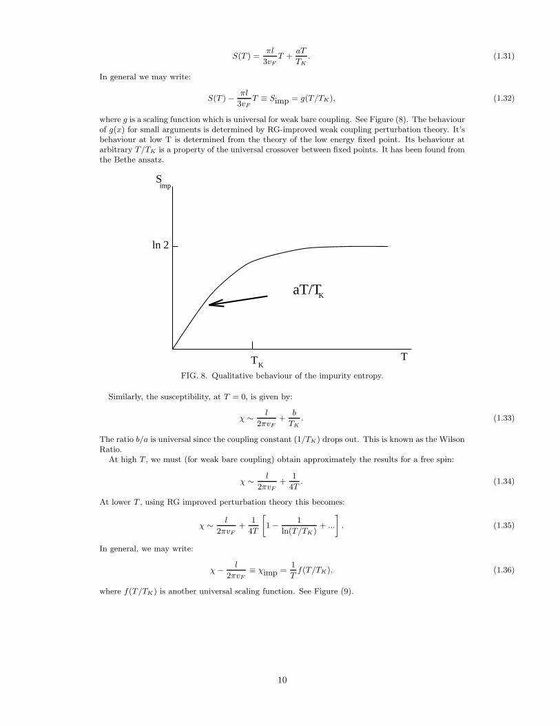
In general, we may write:

χ− l

2πvF≡ χimp =

1

Tf(T/TK), (1.36)

where f(T/TK) is another universal scaling function. See Figure (9).

10

T

K

K

TK

ln (T/T )4T

+...

T

χ

1 - 1

imp

1

b

FIG. 9. Qualitative behaviour of the impurity susceptibility.

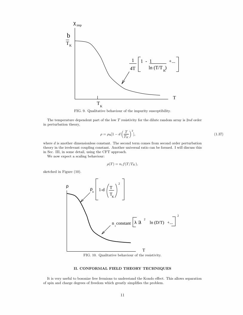
The temperature dependent part of the low T resistivity for the dilute random array is 2nd orderin perturbation theory,

ρ = ρu[1 − d(

T

TK

)2

], (1.37)

where d is another dimensionless constant. The second term comes from second order perturbationtheory in the irrelevant coupling constant. Another universal ratio can be formed. I will discuss thisin Sec. III, in some detail, using the CFT approach.

We now expect a scaling behaviour:

ρ(T ) = nif(T/TK),

sketched in Figure (10).

K

T

λ + λ ln (D/T)2

+...

2

Tu

T

ρ

n i

2

ρ 1-d

constant

FIG. 10. Qualitative behaviour of the resistivity.

II. CONFORMAL FIELD THEORY TECHNIQUES

It is very useful to bosonize free fermions to understand the Kondo effect. This allows separationof spin and charge degrees of freedom which greatly simplifies the problem.

11

We start by considering a left-moving spinless fermion field with Hamiltonian density:

H =1

2πψ†

Lid

dxψL. (2.1)

Define the current (=density) operator,

JL(x− t) = : ψ+LψL : (x, t)

= limǫ→0

[ψL(x)ψL(x+ ǫ) − 〈0|ψL(x)ψL(x+ ǫ)|0〉] (2.2)

(Henceforth we generally drop the subscripts “L”.) We will reformulate the theory in terms ofcurrents (key to bosonization). Consider:

J(x) J(x+ ǫ) as ǫ→ 0

= : ψ†(x)ψ(x)ψ†(x+ ǫ)ψ(x+ ǫ) :

+[: ψ†(x)ψ(x+ ǫ) : + : ψ(x)ψ†(x+ ǫ) :]G(ǫ) +G(ǫ)2

G(ǫ) = 〈0|ψ(x)ψ†(x+ ǫ)|0〉 =1

−iǫ . (2.3)

By Fermi statistics the 4-Fermi term vanishes as ǫ→ 0

: ψ†(x)ψ(x)ψ†(x)ψ(x) : = − : ψ†(x)ψ†(x)ψ(x)ψ(x) : = 0. (2.4)

The second term becomes a derivative,

limǫ→0

[J(x)J(x+ ǫ) +1

ǫ2] = lim

ǫ→0

1

−iǫ [: ψ†(x)ψ(x+ ǫ) : − : ψ†(x+ ǫ) ψ(x) :]

= 2i : ψ† d

dxψ :

H =1

4πJ(x)2 + constant. (2.5)

Now consider the commutator, [J(x), J(y)]. The quartic and quadratic terms cancel. We must becareful about the divergent c-number part,

[J(x), J(y)] = − 1

(x− y − iδ)2+

1

(x− y + iδ)2(δ → 0+)

=d

dx

[

1

x− y − iδ− 1

x− y + iδ

]

= 2πid

dxδ(x− y) (2.6)

Now consider the free massless boson theory with Hamiltonian density (setting vF = 1):

H =1

2

(

∂φ

∂t

)2

+1

2

(

∂φ

∂x

)2

, [φ(x),∂

∂tφ(y)] = iδ(x− y) (2.7)

We can again decompose it into the left and right-moving parts,

(∂t2 − ∂x

2)φ = (∂t + ∂x)(∂t − ∂x)φ

φ(x, t) = φL(x+ t) + φR(x− t)

(∂t − ∂x)φL ≡ ∂−φL = 0, ∂+φR = 0

H =1

4(∂−φ)2 +

1

4(∂+φ)2 =

1

4(∂−φR)2 +

1

4(∂+φL)2 (2.8)

Consider the Hamiltonian density for a left-moving boson field:

H =1

4(∂+φL)2

[∂+φL(x), ∂+φL(y)] = [φ + φ′, φ+ φ′] = 2id

dxδ(x− y) (2.9)

Comparing to the Fermionic case, we see that:

JL =√π∂+φL =

√π∂+φ, (2.10)

12

since the commutation relations and Hamiltonian are the same. That means the operators are thesame with appropriate boundary conditions.

Let’s compare the spectra. For the Fermionic case, choose boundary condition:

ψ(l) = −ψ(−l) (i.e. ψL(l) + ψR(l) = 0), k =π

l(n+

1

2), n = 0,±1,±2... (2.11)

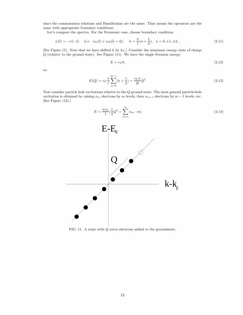
[See Figure (5). Note that we have shifted k by kF .] Consider the minimum energy state of chargeQ (relative to the ground state). See Figure (11). We have the single Fermion energy:

E = vF k, (2.12)

so:

E(Q) = vFπ

l

Q−1∑

n=0

(n+1

2) =

vF π

2lQ2. (2.13)

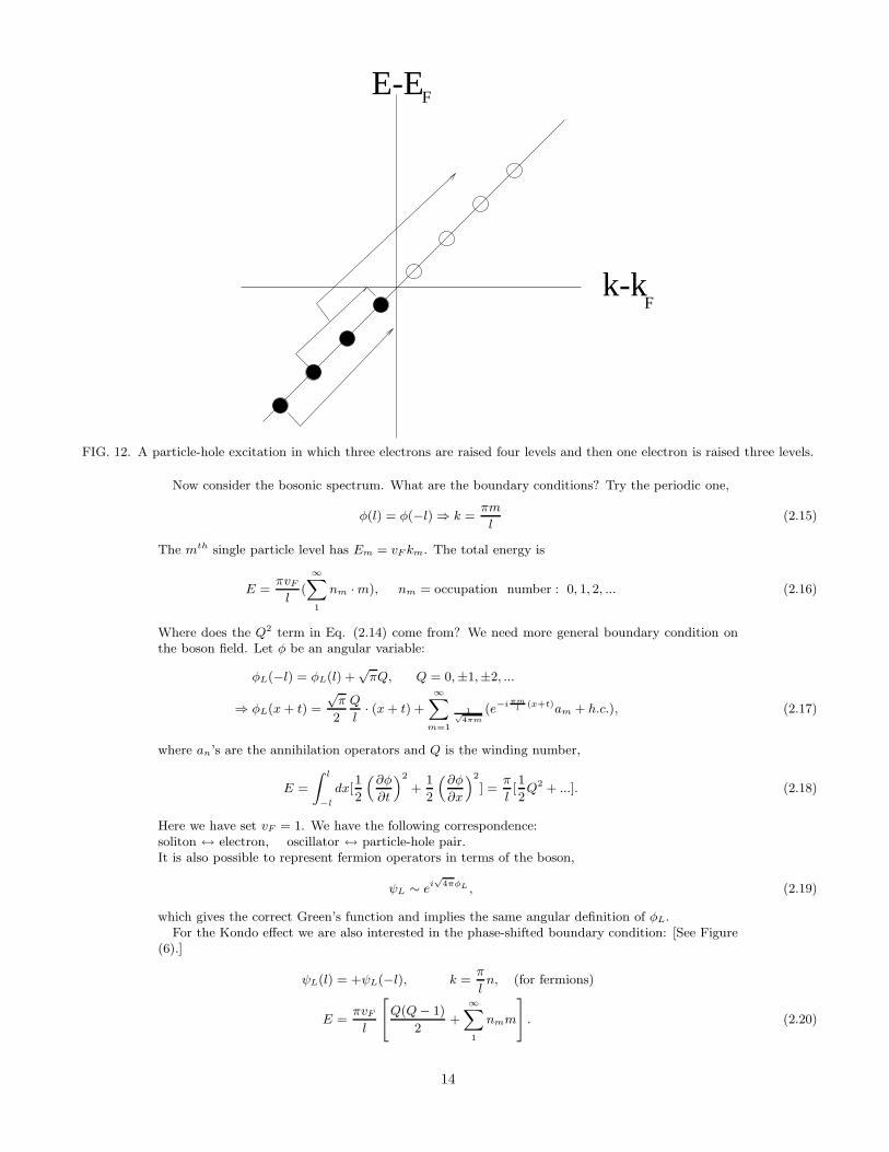
Now consider particle hole excitations relative to the Q-ground state: The most general particle-holeexcitation is obtained by raising nm electrons by m levels, then nm−1 electrons by m− 1 levels, etc.[See Figure (12).]

E =πvF

l(1

2Q2 +

∞∑

m=1

nm ·m) (2.14)

Q

F

F

k-k

E-E

FIG. 11. A state with Q extra electrons added to the groundstate.

13

E-E

k-kF

F

FIG. 12. A particle-hole excitation in which three electrons are raised four levels and then one electron is raised three levels.

Now consider the bosonic spectrum. What are the boundary conditions? Try the periodic one,

φ(l) = φ(−l) ⇒ k =πm

l(2.15)

The mth single particle level has Em = vF km. The total energy is

E =πvF

l(

∞∑

1

nm ·m), nm = occupation number : 0, 1, 2, ... (2.16)

Where does the Q2 term in Eq. (2.14) come from? We need more general boundary condition onthe boson field. Let φ be an angular variable:

φL(−l) = φL(l) +√πQ, Q = 0,±1,±2, ...

⇒ φL(x+ t) =

√π

2

Q

l· (x+ t) +

∞∑

m=1

1√4πm

(e−i πml

(x+t)am + h.c.), (2.17)

where an’s are the annihilation operators and Q is the winding number,

E =

∫ l

−l

dx[1

2

(

∂φ

∂t

)2

+1

2

(

∂φ

∂x

)2

] =π

l[1

2Q2 + ...]. (2.18)

Here we have set vF = 1. We have the following correspondence:soliton ↔ electron, oscillator ↔ particle-hole pair.It is also possible to represent fermion operators in terms of the boson,

ψL ∼ ei√

4πφL , (2.19)

which gives the correct Green’s function and implies the same angular definition of φL.For the Kondo effect we are also interested in the phase-shifted boundary condition: [See Figure

(6).]

ψL(l) = +ψL(−l), k =π

ln, (for fermions)

E =πvF

l

[

Q(Q− 1)

2+

∞∑

1

nmm

]

. (2.20)

14

We have the degenerate ground state, Q = 0 or 1, which correspond to an anti-periodic boundarycondition on φ,

φ(l) = φ(−l) +√π(Q− 1

2)

E =π

l

1

2(Q− 1

2)2 + ... =

π

l(1

2Q(Q− 1) + const. + ...) (2.21)

Now we include spin, i.e. we have 2-component electrons,

H0 = ivFψα† d

dxψα, (α = 1, 2, summed). (2.22)

Now we have charge and spin currents (or densities). We can write H in a manifestly SU(2) invariantway, quadratic in charge and spin currents:

J =: ψα†ψα : , ~J = ψ†α ~σβα

2ψβ (2.23)

Using:

~σβα · ~σδ

γ = 2δβγ δ

δα − δα

β δγδ (2.24)

~J2 = −3

4: ψ†αψαψ

†βψβ : +3i

2ψα+ d

dxψα + c-number,

J2 = : ψ†αψαψ†βψβ : +2iψα+ d

dxψα + c-number,

H =1

8πJ2 +

1

6π~J2, (2.25)

we have the following commutation relations,

[J(x), J(y)] = 4πiδ′(x− y), (twice the result for the spinless case)

[J(x), Jz(y)] =1

2[J↑ + J↓, J↑ − J↓] = 0. (2.26)

From [J, ~J ] = 0, we see that H is sum of commuting charge and spin parts.

[Ja(x), Jb(y)] = 2πψ†[σ

2

a,σ

2

b]ψ · δ(x− y) + tr[

σ

2

a,σ

2

b]2πi

d

dxδ(x− y)

= 2πiǫabcJc(x) · δ(x− y) + πiδab d

dxδ(x− y). (2.27)

We obtain the Kac-Moody algebra of central charge k = 1. More generally the coefficient of thesecond term is multiplied by an integer k.Fourier transforming,

~Jn ≡ 1

2π

∫ l

−l

dxein πl

x ~J(x), [Jan , J

bm] = iǫabcJc

n+m +1

2nδabδn,−m (2.28)

we have an ∞-dimensional generalization of the ordinary SU(2) Lie algebra. The spin part of theHamiltonian is

Hs =π

l

1

3

∞∑

n=−∞

: ~J−n · ~Jn : (2.29)

The spectrum of Hs is again determined by the algebra obeyed by the ~Jn’s together with boundaryconditions. The construction is similar to building representations of SU(2) from commutationrelations, i.e. constructing raising operator, etc.

In the k = 1 case we are considering here it is simplest to use:

~J(x)2 = 3(Jz(x))2

H =1

8πJ2 +

1

2π(Jz)2

=1

4π(J2

↑ + J2↓ )

=1

4((∂+φ↑)

2 + (∂+φ↓)2)

=1

4[(∂+(

φ↑ + φ↓√2

))2 + (∂+(φ↑ − φ↓√

2))2]

=1

4((∂+φc)

2 + (∂+φs)2) (2.30)

15

Now we have introduced two commuting charge and spin free massless bosons. SU(2) symmetry isnow concealed but boundary condition on φs must respect it. Consider the spectrum of fermiontheory with boundary condition: ψ(l) = −ψ(−l),

E =πV

l

[

Q↑2

2

+Q↓2

2

+

∞∑

m=−∞

m(n↑m + n↓

m)

]

. (2.31)

Change over to φc and φs. We can relabel occupation numbers,

n↑m, n

↓m −→ nc

m, nsm

Q = Q↑ +Q↓

Sz =1

2(Q↑ −Q↓)

E =πvF

l[1

4Q2 + (Sz)2 +

∞∑

1

mncm +

∞∑

1

mnsm] (2.32)

= Ec + Es

φc =

√π

2√

2

Q

l(x+ t) + ...

φs =π√2

Sz

l(x+ t) + ... (2.33)

Actually charge and spin bosons are not completely decoupled; we must require Q = 2Sz (mod 2),to correctly reproduce the free fermion spectrum. We see that the boundary conditions on φc andφc are coupled. Now consider the phase-shifted case.

E =πvF

l[1

4(Q− 1)2 + (Sz)2 + ...] (2.34)

Redefine Q− 1 → Q so

E =πvF

l[1

4Q2 + (Sz)2 + ....], (2.35)

the same as before the phase shift, Eq. (2.32). One of the 0-energy single-particle states is filled,for Q = 0 and there are 4 groundstates,

(Q,Sz) = (0,±1

2), (±1, 0). (2.36)

Now Q = 2Sz +1 (mod 2); i.e. we “glue” together charge and spin excitations in two different ways,either

(even, integer) ⊕ (odd, half-integer)

or (even, half-integer) ⊕ (odd, integer), (2.37)

depending on the boundary conditions. The π2

phase shift simply reverses these “gluing conditions”.The set of all integer spin states form a “conformal tower”. They can be constructed from the Kac-

Moody algebra by applying the raising operators ~J−n to the lowest (singlet) state, with all spacingsπvF

l·(integer). Likewise for all half-integer spin states, (sz)2 = 1

4+integer. Likewise for even and

odd charge states. The K-M algebra determines uniquely conformal towers but boundary conditionsdetermine which conformal towers occur in the spectrum and in which spin-charge combinations.

III. CONFORMAL FIELD THEORY APPROACH TO THE KONDO EFFECT

The chiral one-dimensional Hamiltonian density of Eq. (1.19) and (1.14) is:

H =d

dxψLα + λψ†α

L

~σβα

2ψLβ · ~S δ(x) (left-movers only) (3.1)

We rewrite it in terms of spin and charge currents only,

H =1

8πJ2 +

1

6π( ~J)2 + λ~J · ~S δ(x). (3.2)

16

The Kondo interaction involves spin fields only, not charge fields: H = Hs +Hc. Henceforth we onlyconsider the spin part. In Fourier transformed form,

Hs =π

l(1

3

∞∑

n=−∞

~J−n · ~Jn + λ

∞∑

n=−∞

~Jn · ~S)

[Jan , J

bm] = iǫabcJc

n+m +n

2δabδn,−m

[Sa, Sb] = iǫabcSc

[Sa, Jbn] = 0 (3.3)

From calculating Green’s functions for ~J(x) we could again reproduce perturbation theory dλdlnD

=−λ2 + · · ·. That is a small λ > 0 grows. What is the infrared stable fixed point? Consider λ = 2

3,

where we may “complete the square”.

H =πV

3l

∞∑

n=−∞

[( ~J−n + ~S) · ( ~Jn + ~S) − 3

4]

[Jan + Sa, Jb

m + Sb] = iǫabc(Jcn+m + Sc) +

n

2δabδn,−m. (3.4)

H is quadratic in the new currents, ~Jn ≡ ~Jn + ~S, which obey the same Kac-Moody algebra! Whatis the spectrum of H(λ = 2

3)? We must get back to Kac-Moody conformal towers for integer and

half-integer spin. This follows from the KM algebra and the form of H (i.e. starting from the loweststate we produce the entire tower by applying the raising operators, ~J−n).

Thus we find that the strong-coupling fixed point is the same as the weak-coupling fixed point.However, the total spin operator is now ~J0 = ~J0 + ~S. We consider impurity spin magnitude, s=1/2.Any integer-spin state becomes a 1/2-integer spin state and vice versa.

Integer ↔ 1/2-Integer. (3.5)

Presumably λ = 2/3 is the strong coupling fixed point in this formulation of the problem. ∞-coupling can become finite coupling under a redefinition, eg.

λLattice =λKM

1 − 32λKM

. (3.6)

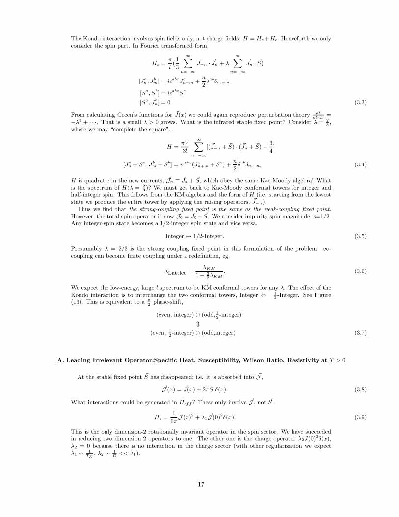
We expect the low-energy, large l spectrum to be KM conformal towers for any λ. The effect of theKondo interaction is to interchange the two conformal towers, Integer ⇔ 1

2-Integer. See Figure

(13). This is equivalent to a π2

phase-shift,

(even, integer) ⊕ (odd, 12-integer)

m(even, 1

2-integer) ⊕ (odd,integer) (3.7)

A. Leading Irrelevant Operator:Specific Heat, Susceptibility, Wilson Ratio, Resistivity at T > 0

At the stable fixed point ~S has disappeared; i.e. it is absorbed into ~J ,

~J (x) = ~J(x) + 2π~S δ(x). (3.8)

What interactions could be generated in Heff? These only involve ~J , not ~S.

Hs =1

6π~J (x)2 + λ1

~J (0)2δ(x). (3.9)

This is the only dimension-2 rotationally invariant operator in the spin sector. We have succeededin reducing two dimension-2 operators to one. The other one is the charge-operator λ2J(0)2δ(x),λ2 = 0 because there is no interaction in the charge sector (with other regularization we expectλ1 ∼ 1

TK, λ2 ∼ 1

D<< λ1).

17

1/2 integer-s

tower tower

integer-s

FIG. 13. At λ = 2/3 the 1/2-integer-spin conformal tower is mapped into the integer-spin conformal tower.

Now we calculate the specific heat and susceptibility to 1st order in λ1.Susceptibility of left-moving free fermions:

0-th order M =1

2(n↑ − n↓) = l

∫

dǫ ν(ǫ)[n(ǫ+h

2) − n(ǫ− h

2)]

χ =l

2π(for T << D)

1st order χ =1

3T〈[∫

dx ~J (x)]2〉λ1

= χ0 − λ1

3T 2〈[∫

dx ~J (x)]2 ~J (0)2〉 + ... (3.10)

A simplifying trick is to replace:

δH = λ1~J 2(0)δ(x) −→ λ1

2l~J 2(x), (3.11)

which gives the same result to first order in λ (only) by translational invariance of H at λ = 0. Nowthe Hamiltonian density changes into

H → (1

6π+λ1

2l) ~J 2(x). (3.12)

We simply rescale H by a factor

H → (1 +3πλ1

l)H. (3.13)

Equivalently in a thermal average,

T → T

1 + 3πλ1l

≡ T (λ1) (3.14)

χ(λ1, T ) =1

3T< (

∫

~J )2 >T (λ1)

=1

1 + 3πλ1/lχ(0, T (λ1))

≈ [1 − 3πλ1

l]χ0

=l

2π− 3λ1

2, (3.15)

18

where in the last equality the first term represents the bulk part and the second one, of order ∼ 1TK

,comes from the impurity part. Specific Heat:

0-th order C = Cc +Cs, Cc = Cs =πlT

3. (3.16)

Each free left-moving boson makes an identical contribution.

1st order in λ1 Cs(λ1, T ) =∂

∂T< H(λ1) >λ1

= Cs(0, T (λ1))

=πl

3

T

1 + 3πλ1/l

≈ πlT

3− π2λ1T (3.17)

δCs

Cs= −3πλ1

l= 2

δCs

C(3.18)

The Wilson Ratio:

Rw ≡ δχ/χ

δC/C= 2 =

C

Cs(3.19)

measues the fraction of C coming from the spin degrees of freedom.Doing more work, we can calculate the resistivity to O(λ2).7,15 First we get the electron lifetime

from the self-energy. The change in the 3D Green’s function comes only from the 1D s-wave part:

G3(~r1, ~r2) −G03(|~r1 − ~r2|)

=1

8π2r1r2[e−ikF (r1+r2)(GLR(r1, r2) −GLR,0(r1, r2)) + h.c.]

= G03(r1)ΣG

03(r2). (3.20)

The self-energy Σ depends only on the frequency. It gets multiplied by the impurity concentationfor a finite density (in the dilute limit). We must calculate the 1D Green’s function GLR(r1, r2, ω)perturbatively in λ

O(λ01) : GLR(r1, r2) = −G0

LL(r1,−r2)= −G0

LL(r1 + r2)

= −G0LR(r1, r2), (3.21)

where the (−) sign comes from the change in boundary conditions,

GLR −G0LR = −2G0

LR +O(λ1) (3.22)

To calculate to higher orders it is convenient to write the interaction as:

~J 2 = −3

4: ψ†αψαψ

†βψβ : +3i

4(ψ†α d

dxψα − dψ†α

dxψα) (3.23)

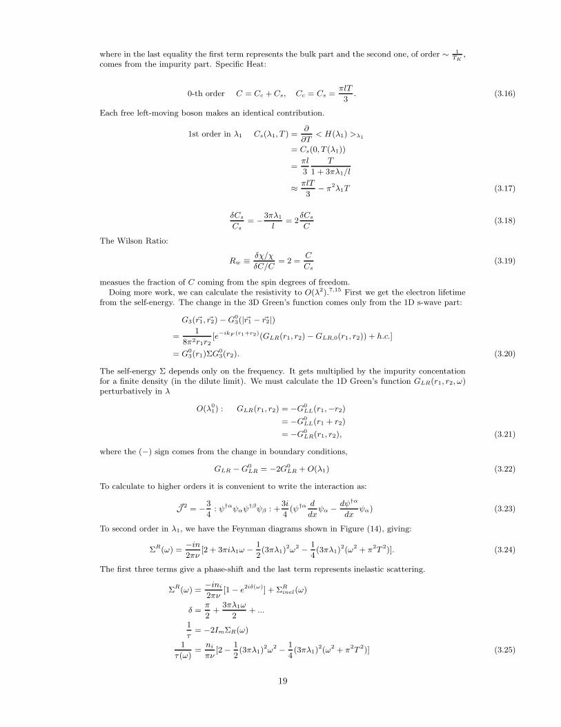
To second order in λ1, we have the Feynman diagrams shown in Figure (14), giving:

ΣR(ω) =−in2πν

[2 + 3πiλ1ω − 1

2(3πλ1)

2ω2 − 1

4(3πλ1)

2(ω2 + π2T 2)]. (3.24)

The first three terms give a phase-shift and the last term represents inelastic scattering.

ΣR(ω) =−ini

2πν[1 − e2iδ(ω)] + ΣR

inel(ω)

δ =π

2+

3πλ1ω

2+ ...

1

τ= −2ImΣR(ω)

1

τ (ω)=ni

πν[2 − 1

2(3πλ1)

2ω2 − 1

4(3πλ1)

2(ω2 + π2T 2)] (3.25)

19

The leading λ1 dependence is O(λ21) in this case. The O(λ1) term in ΣR is real. We calculate the

conductivity from the Kubo formula. (There is no contribution from the scattering vertex for pures-wave scattering.)

σ(T ) =2e2

3m3

∫

d3~k

(2π)3

[

− ∂n

∂ǫk

]

~k2τ (ǫk)

τ (ǫk) ≈ πν

2ni[1 +

1

4(3πλ1

2)ǫ2k +1

8(3πλ1)

2(ǫ2k + (π2T 2)]

ρ(T ) =1

σ(T )=

3ni

π(evF ν)2[1 − 9

4π4λ2

1T2] (3.26)

All low-temperature properties are determined in terms of one unknown coupling constant λ1 ∼ 1TK

.

Numerical or Bethe ansatz methods are needed to find the precise value of λ1(D, λ) ∝ 1De1/λ.

FIG. 14. Feynman diagrams contributing to the electron self-energy up to second order in the leading irrelevant couplingconstant of Eq. (3.8).

IV. MULTI-CHANNEL KONDO EFFECT

Normally there are several “channels” of electrons -e.g. different d-shell orbitals. A very simpleand symmetric model is:

H =∑

~k,α,i=1,2,...k

ǫ~kψ†αi~k

ψ~kαi + λ~S ·∑

~k,~k′α,βi

ψ†αi~k~σβ

αψ~k′βi. (4.1)

This model has SU(2)×SU(k)×U(1) symmetry. Realistic systems do not have this full symmetry.To understand the potential applicability of this model we need to analyse the relevance of varioustypes of symmetry breaking.14 An interesting possible experimental application of the model wasproposed by Ralph, Ludwig, von Delft and Buhrman.19 In general, we let the impurity have anarbitrary spin, s, as well.

Perturbation theory in λ is similar to the result mentioned before:

dλ

d lnD= −νλ2 +

k

2ν2λ3 +O[ks(s+ 1)λ4]

~S2 = s(s+ 1). (4.2)

Does λ → ∞ as T → 0? Let’s suppose it does and check consistency. What is the groundstate forthe lattice model of Eq. (1.20), generalized to arbitrary k and s, at λ/t → ∞? In the limit we justconsider the single-site model:

H = λ~S · ψ†0

~σ

2ψ0, (4.3)

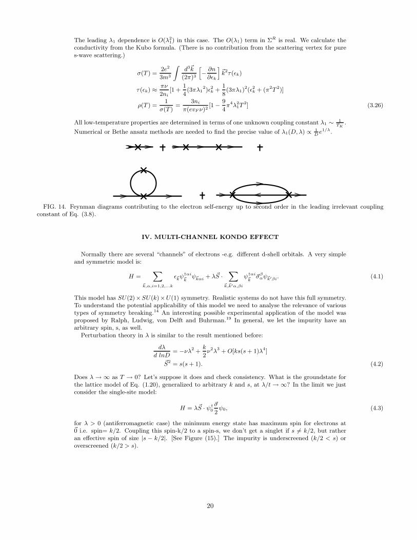
for λ > 0 (antiferromagnetic case) the minimum energy state has maximum spin for electrons at~0 i.e. spin= k/2. Coupling this spin-k/2 to a spin-s, we don’t get a singlet if s 6= k/2, but ratheran effective spin of size |s − k/2|. [See Figure (15).] The impurity is underscreened (k/2 < s) oroverscreened (k/2 > s).

20

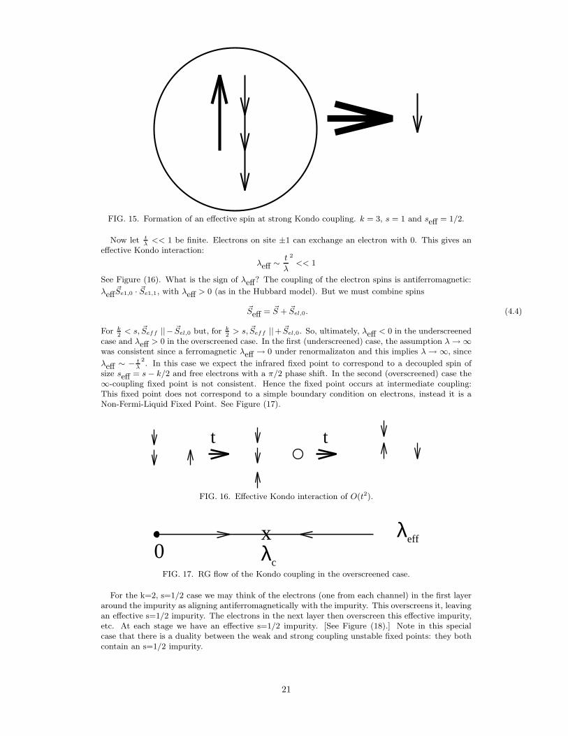
FIG. 15. Formation of an effective spin at strong Kondo coupling. k = 3, s = 1 and seff = 1/2.

Now let tλ<< 1 be finite. Electrons on site ±1 can exchange an electron with 0. This gives an

effective Kondo interaction:

λeff ∼ t

λ

2

<< 1

See Figure (16). What is the sign of λeff? The coupling of the electron spins is antiferromagnetic:

λeff~Se1,0 · ~Se1,1, with λeff > 0 (as in the Hubbard model). But we must combine spins

~Seff = ~S + ~Sel,0. (4.4)

For k2< s, ~Seff ||− ~Sel,0 but, for k

2> s, ~Seff ||+ ~Sel,0. So, ultimately, λeff < 0 in the underscreened

case and λeff > 0 in the overscreened case. In the first (underscreened) case, the assumption λ→ ∞was consistent since a ferromagnetic λeff → 0 under renormalizaton and this implies λ → ∞, since

λeff ∼ − tλ

2. In this case we expect the infrared fixed point to correspond to a decoupled spin of

size seff = s− k/2 and free electrons with a π/2 phase shift. In the second (overscreened) case the∞-coupling fixed point is not consistent. Hence the fixed point occurs at intermediate coupling:This fixed point does not correspond to a simple boundary condition on electrons, instead it is aNon-Fermi-Liquid Fixed Point. See Figure (17).

tt

FIG. 16. Effective Kondo interaction of O(t2).

λeff

0xλc

FIG. 17. RG flow of the Kondo coupling in the overscreened case.

For the k=2, s=1/2 case we may think of the electrons (one from each channel) in the first layeraround the impurity as aligning antiferromagnetically with the impurity. This overscreens it, leavingan effective s=1/2 impurity. The electrons in the next layer then overscreen this effective impurity,etc. At each stage we have an effective s=1/2 impurity. [See Figure (18).] Note in this specialcase that there is a duality between the weak and strong coupling unstable fixed points: they bothcontain an s=1/2 impurity.

21

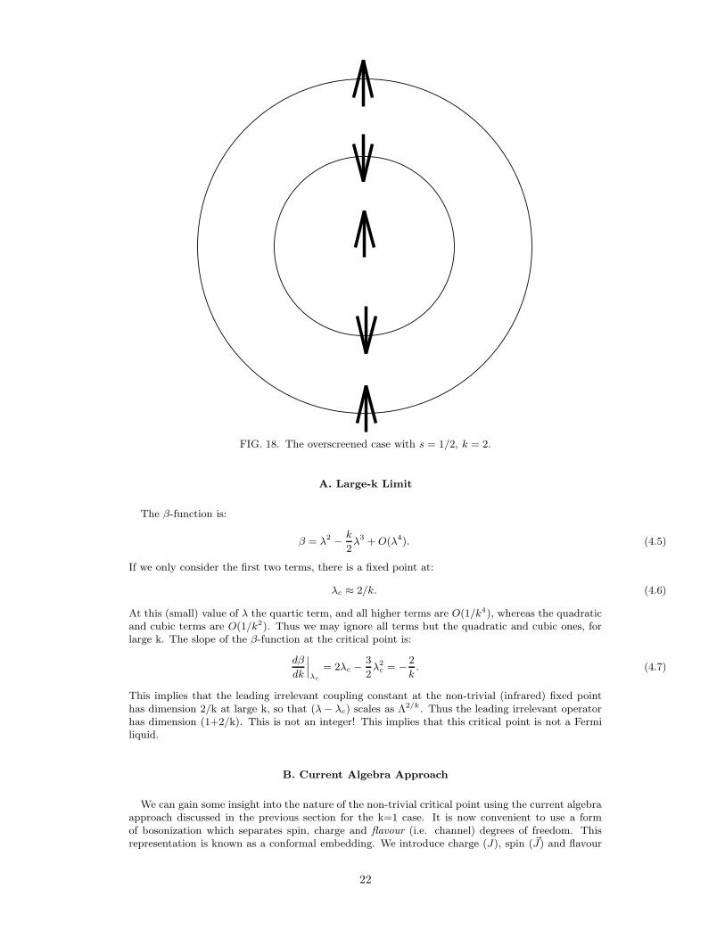
FIG. 18. The overscreened case with s = 1/2, k = 2.

A. Large-k Limit

The β-function is:

β = λ2 − k

2λ3 +O(λ4). (4.5)

If we only consider the first two terms, there is a fixed point at:

λc ≈ 2/k. (4.6)

At this (small) value of λ the quartic term, and all higher terms are O(1/k4), whereas the quadraticand cubic terms are O(1/k2). Thus we may ignore all terms but the quadratic and cubic ones, forlarge k. The slope of the β-function at the critical point is:

dβ

dk

∣

∣

∣

λc

= 2λc − 3

2λ2

c = − 2

k. (4.7)

This implies that the leading irrelevant coupling constant at the non-trivial (infrared) fixed pointhas dimension 2/k at large k, so that (λ− λc) scales as Λ2/k. Thus the leading irrelevant operatorhas dimension (1+2/k). This is not an integer! This implies that this critical point is not a Fermiliquid.

B. Current Algebra Approach

We can gain some insight into the nature of the non-trivial critical point using the current algebraapproach discussed in the previous section for the k=1 case. It is now convenient to use a formof bosonization which separates spin, charge and flavour (i.e. channel) degrees of freedom. Thisrepresentation is known as a conformal embedding. We introduce charge (J), spin ( ~J) and flavour

22

(JA) currents. A runs over the k2 − 1 generators of SU(k). The corresponding elements of thealgebra are written TA. These are traceless Hermitean matrices normalized so that:

trTATB =1

2δAB, (4.8)

and obeying the completeness relation:∑

A

(TA)ba(TA)d

c =1

2

[

δbcδ

da − 1

kδb

aδdc

]

, (4.9)

and the commutation relations:

[TA, TB ] = ifABCTC , (4.10)

where the fABC are the SU(k) structure constants. Thus the currents are:

J ≡ : ψ†iαψiα :

~J ≡ ψ†iα ~σβα

2ψiβ

JA ≡ ψ†iα(TA)jiψjα. (4.11)

(All repeated indices are summed.) It can be seen using Eq. (4.9) that the free fermion Hamiltoniancan be written in terms of these currents as:

H =1

8πkJ2 +

1

2π(k + 2)~J2 +

1

2π(k + 2)JAJA. (4.12)

The currents ~J obey the SU(2) Kac-Moody algebra with central charge k and the currents JA obeythe SU(k) Kac-Moody algebra with central charge 2:

[JAn , J

Bm] = ifABCJC

n+m + nδABδn,−m. (4.13)

The three types of currents commute with each of the other two types, as do the three parts of theHamiltonian. Thus we have succeeded in expressing the Hamiltonian in terms of these three typesof excitations: charge, spin and flavour. The Virasoro central charge c (proportional to the specificheat) for a Hamiltonian quadratic in currents of a general group G at level k is:26

cG,k =Dim(G) · kCV (G) + k

, (4.14)

where Dim (G) is the dimension of the group and CV (G) is the quadratic Casimir in the fundamentalrepresentation. For SU(k) this has the value:

CV (SU(k)) = k. (4.15)

Thus the total value of the central charge, c, is:

cTOT = 1 +3 · kk + 2

+(k2 − 1) · 2k + 2

= 2k, (4.16)

the correct value for 2k species of free fermions. Complicated “gluing conditions” must be imposed tocorrectly reproduce the free fermion spectra, with various boundary conditions. These were workedout in general by Altshuler, Bauer and Itzykson.27 The SU(2)k sector consists of k + 1 conformaltowers, labelled by the spin of the lowest energy (“highest weight”) state: s = 0, 1/2, 1, ...k/2.32,33

We may now treat the Kondo interaction much as in the single channel case. It only involves thespin sector which now becomes:

Hs =1

2π(k + 2)~J2 + λ~J · ~Sδ(x). (4.17)

We see that we can always “complete the square” at a special value of λ:

λc =2

2 + k, (4.18)

where the Hamiltonian reduces to its free form after a shift of the current operators by ~S whichpreserves the KM algebra. We note that at large k this special value of λ reduces to the onecorresponding to the critical point: λc → 2/k.

While this observation is tantalizing, it leaves many open questions. We might expect that somerearranging of the (k + 1) SU(2)k conformal towers takes place at the critical point but preciselywhat is it? Does it correspond to some sort of boundary condition? If so what? How can wecalculate thermodynamic quantities and Green’s functions? To answer these questions we need tounderstand some more technical aspects of CFT in the presence of boundaries.

23

V. BOUNDARY CONFORMAL FIELD THEORY

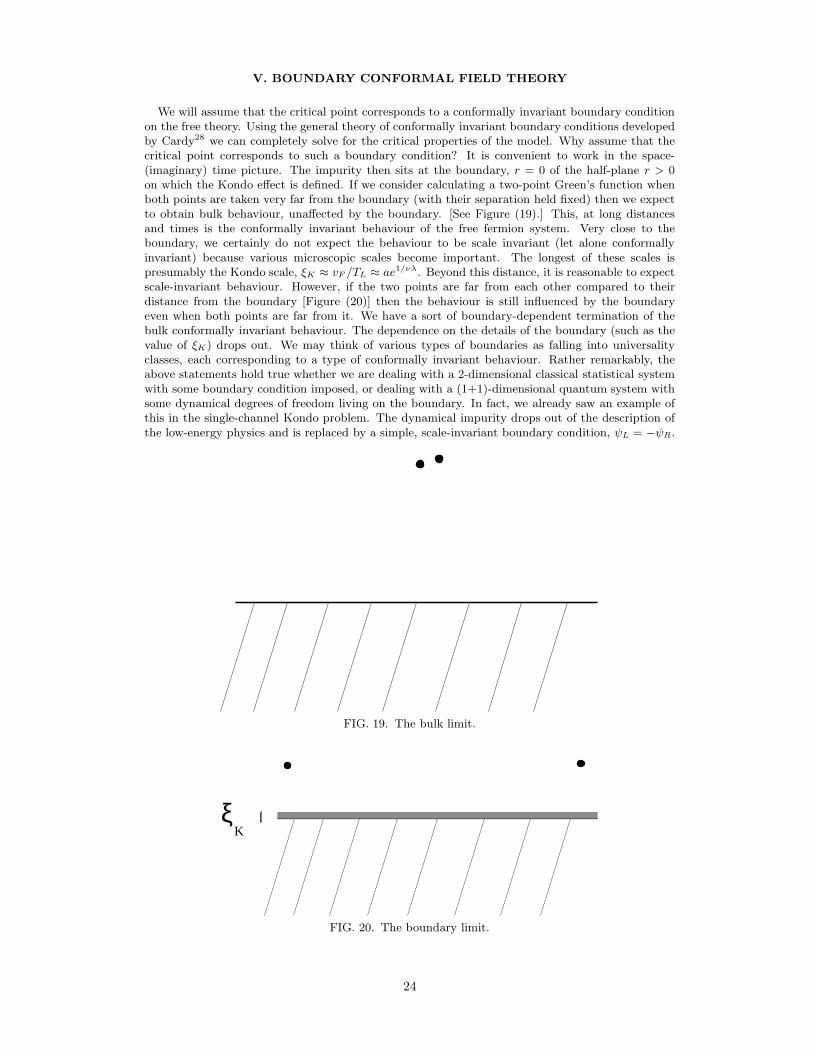
We will assume that the critical point corresponds to a conformally invariant boundary conditionon the free theory. Using the general theory of conformally invariant boundary conditions developedby Cardy28 we can completely solve for the critical properties of the model. Why assume that thecritical point corresponds to such a boundary condition? It is convenient to work in the space-(imaginary) time picture. The impurity then sits at the boundary, r = 0 of the half-plane r > 0on which the Kondo effect is defined. If we consider calculating a two-point Green’s function whenboth points are taken very far from the boundary (with their separation held fixed) then we expectto obtain bulk behaviour, unaffected by the boundary. [See Figure (19).] This, at long distancesand times is the conformally invariant behaviour of the free fermion system. Very close to theboundary, we certainly do not expect the behaviour to be scale invariant (let alone conformallyinvariant) because various microscopic scales become important. The longest of these scales ispresumably the Kondo scale, ξK ≈ vF /TL ≈ ae1/νλ. Beyond this distance, it is reasonable to expectscale-invariant behaviour. However, if the two points are far from each other compared to theirdistance from the boundary [Figure (20)] then the behaviour is still influenced by the boundaryeven when both points are far from it. We have a sort of boundary-dependent termination of thebulk conformally invariant behaviour. The dependence on the details of the boundary (such as thevalue of ξK) drops out. We may think of various types of boundaries as falling into universalityclasses, each corresponding to a type of conformally invariant behaviour. Rather remarkably, theabove statements hold true whether we are dealing with a 2-dimensional classical statistical systemwith some boundary condition imposed, or dealing with a (1+1)-dimensional quantum system withsome dynamical degrees of freedom living on the boundary. In fact, we already saw an example ofthis in the single-channel Kondo problem. The dynamical impurity drops out of the description ofthe low-energy physics and is replaced by a simple, scale-invariant boundary condition, ψL = −ψR.

FIG. 19. The bulk limit.

Kξ

FIG. 20. The boundary limit.

24

Precisely what is meant by a conformally invariant boundary condition? Without boundaries,conformal transformations are analytic mappings of the complex plane:

z ≡ τ + ix, (5.1)

into itself:

z → w(z). (5.2)

(Henceforth, we set the Fermi velocity, vF = 1.) We may Taylor expand an arbitrary conformaltransformation around the origin:

w(z) =

∞∑

0

anzn, (5.3)

where the an’s are arbitrary complex coefficients. They label the various generators of the conformalgroup. It is the fact that there is an infinite number of generators (i.e. coefficients) which makesconformal invariance so powerful in (1+1) dimensions. Now suppose that we have a boundary atx = 0, the real axis. At best, we might hope to have invariance under all transformations whichleave the boundary fixed. This implies the condition:

w(τ )∗ = w(τ ). (5.4)

We see that there is still an infinite number of generators, corresponding to the an’s of Eq. (5.3)except that now we must impose the conditions:

a∗n = an. (5.5)

We have reduced the (still ∞) number of generators by a factor of 1/2. The fact that there is still an∞ number of generators, even in the presence of a boundary, means that this boundary conformalsymmetry remains extremely powerful.

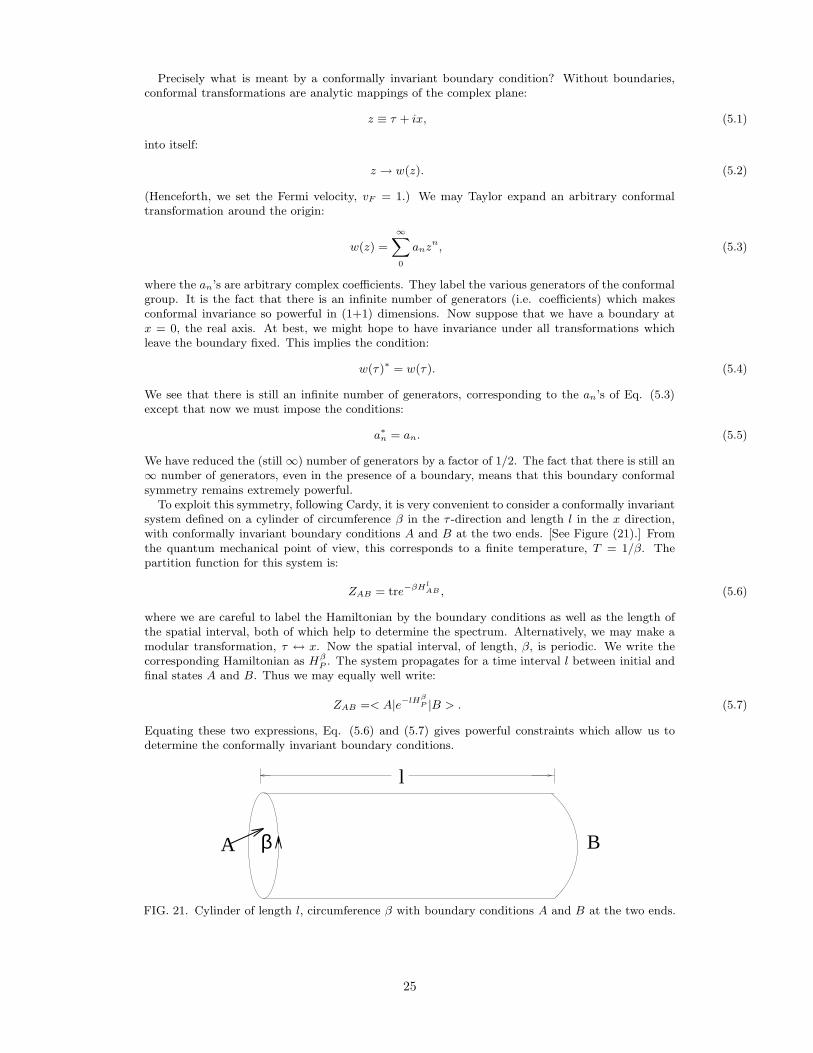
To exploit this symmetry, following Cardy, it is very convenient to consider a conformally invariantsystem defined on a cylinder of circumference β in the τ -direction and length l in the x direction,with conformally invariant boundary conditions A and B at the two ends. [See Figure (21).] Fromthe quantum mechanical point of view, this corresponds to a finite temperature, T = 1/β. Thepartition function for this system is:

ZAB = tre−βHlAB , (5.6)

where we are careful to label the Hamiltonian by the boundary conditions as well as the length ofthe spatial interval, both of which help to determine the spectrum. Alternatively, we may make amodular transformation, τ ↔ x. Now the spatial interval, of length, β, is periodic. We write thecorresponding Hamiltonian as Hβ

P . The system propagates for a time interval l between initial andfinal states A and B. Thus we may equally well write:

ZAB =< A|e−lHβ

P |B > . (5.7)

Equating these two expressions, Eq. (5.6) and (5.7) gives powerful constraints which allow us todetermine the conformally invariant boundary conditions.

β B

l

A

FIG. 21. Cylinder of length l, circumference β with boundary conditions A and B at the two ends.

25

To proceed, we make a further weak assumption about the boundary conditions of interest. Weassume that the momentum density operator, T − T vanishes at the boundary. This amounts to atype of unitarity condition. In the free fermion theory this becomes:

ψ†αiL ψLαi(t, 0) − ψ†αi

R ψRαi(t, 0) = 0. (5.8)

Note that this is consistent with both boundary conditions that occured in the one-channel Kondoproblem: ψL = ±ψR.

Since T (t, x) = T (t+ x) and T (t, x) = T (t− x), it follows that

T (t, x) = T (t,−x). (5.9)

i.e. we may regard T as the analytic continuation of T to the negative axis. Thus, as in ourprevious discussion, instead of working with left and right movers on the half-line we may work withleft-movers only on the entire line. Basically, the energy momentum density, T is unaware of theboundary condition. Hence, in calculating the spectrum of the system with boundary conditions Aand B introduced above, we may regard the system as being defined periodically on a torus of length2l with left-movers only. The conformal towers of T are unaffected by the boundary conditions, A,B. However, which conformal towers occur does depend on these boundary conditions. We introducethe characters of the Virasoro algebra, for the various conformal towers:

χa(e−πβ/l) ≡∑

i

e−βEai(2l), (5.10)

where Eai (2l) are the energies in the ath conformal tower for length 2l. i.e.:

Eai (2l) =

π

lxa

i − πc

24l, (5.11)

where the xai ’s correspond to the (left) scaling dimensions of the operators in the theory and c is the

conformal anomaly. The spectrum of H lAB can only consist of some combination of these conformal

towers. i.e.:

ZAB =∑

a

naABχa(e−πβ/l), (5.12)

where the naAB are some non-negative integers giving the multiplicity with which the various con-

formal towers occur. Importantly, only these multiplicities depend on the boundary conditions, notthe characters, which are a property of the bulk left-moving system. Thus, a specification of allpossible multiplicities, na

AB amounts to a specification of all possible boundary conditions A. Theproblem of specifying conformally invariant boundary conditions has been reduced to determiningsets of integers, na

AB . For rational conformal field theories, where the number of conformal towersis finite, only a finite number of integers needs to be specified.

Now let us focus on the boundary states, |A >. These must obey the operator condition:

[T (x) − T (x)]|A >= 0 (∀x). (5.13)

Fourier transforming with respect to x, this becomes:

[Ln − Ln]|A >= 0. (5.14)

This implies that all boundary states, |A > must be linear combinations of the “Ishibashi states”:29

|a >≡∑

m

|a;m > ⊗|a;m >. (5.15)

Here m labels all states in the ath conformal tower. The first and second factors in Eq. (5.15) referto the left and right-moving sectors of the Hilbert Space. Thus we may write:

|A >=∑

a

|a >< a0|A > . (5.16)

Here,

|a0 >≡ |a; 0 > ⊗|a; 0 >. (5.17)

26

(Note that while the states, |a;m > ⊗|b;n > form a complete orthonormal set, the Ishibashi states,|a > do not have finite norm.) Thus, specification of boundary states is reduced to determining thematrix elements, < a0|A >. (For rational conformal field theories, there is a finite number of suchmatrix elements.) Thus the partition function becomes:

ZAB =∑

a

< A|a0 >< a0|B >< a|e−lHβ

P |a > . (5.18)

From the definition of the Ishibashi state, |a > we see that:

< a|e−lHβ

P |a >=∑

m

e−2lEam(β), (5.19)

the factor of 2 in the exponent arising from the equal contribution to the energy from T and T .This can be written in terms of the characters:

< a|e−lHβ

P |a >= χa(e−4πl/β). (5.20)

We are now in a position to equate these two expressions for ZAB :

ZAB =∑

a

< A|a0 >< a0|B > χa(e−4πl/β) =∑

a

naABχa(e−πβ/l). (5.21)

This equation must be true for all values of l/β. It is very convenient to use the modular transfor-mation of the characters:30,31

χa(e−πβ/l) =∑

b

Sbaχb(e

−4πl/β). (5.22)

Here Sab is known as the “modular S-matrix”. (This name is rather unfortunate since this matrix

has no connection with the scattering-matrix.) We thus obtain a set of equations relating themultiplicities, na

AB which determine the spectrum for a pair of boundary conditions and the matrixelements < a0|A > determining the boundary states:

∑

b

Sab n

bAB =< A|a0 >< a0|B > . (5.23)

We refer to these as Cardy’s equations. They basically allow a determination of the boundary statesand spectrum.

How do we go about constructing boundary states and multiplicities which satisfy these equations?Generally, boundary states corresponding to trivial boundary conditions can be found by inspection.i.e., given nb

AA we can find < a|A >. We can then generate new (sometimes non-trivial) boundarystates by fusion. i.e. given any conformal tower, c, we can obtain a new boundary state |B > andnew spectrum na

AB from the “fusion rule coefficients”, Ncab. These non-negative integers are defined

by the operator product expansion (OPE) for (chiral) primary operators, φa. In general the (OPE)of φa with φb contains the operator φc N

cab times. In simple cases, such as occur in the Kondo

problem, the Ncab’s are all 0 or 1. In the case of SU(2)k, which will be relevant for the Kondo

problem, the OPE is:32,33

j ⊗ j′ = |j − j′|, |j − j′| + 1, |j − j′| + 2, . . . ,min{j + j′, k − j − j′}. (5.24)

Note that this generalizes the ordinary angular momentum addition rules in a way which is consistentwith the conformal tower structure of the theories (i.e. the fact that primaries only exist withj ≤ k/2). Thus,

Nj′′

jj′ = 1 (|j − j′| ≤ j′′ ≤ min{j + j′, k − j − j′}= 0 otherwise. (5.25)

The new boundary state, |B >, and multiplicities obtained by fusion with the conformal tower care given by:

< a0|B > = < a0|A >Sa

c

Sa0

naAB =

∑

b

Nabcn

bAA. (5.26)

27

Here 0 labels the conformal tower of the identity operator. Importantly, the new boundary stateand multiplicities so obtained, obey Cardy’s equation. The right-hand side of Eq. (5.23) becomes:

< A|a0 >< a0|B >=< A|a0 >< a0|A >Sa

c

Sa0

. (5.27)

The left-hand side becomes:∑

b

Sab n

bAB =

∑

b,d

SabN

bdcn

dAA. (5.28)

We now use a remarkable identity relating the modular S-matrix to the fusion rule coefficients,known as the Verlinde formula:34

∑

b

SabN

bdc =

SadS

ac

Sa0

. (5.29)

This gives:

∑

b

Sab n

bAB =

Sac

Sa0

∑

d

Sadn

dAA =

Sac

Sa0

< A|a0 >< a0|A >=< A|a0 >< a0|B >, (5.30)

proving that fusion does indeed give a new solution of Cardy’s equations. The multiplicities, naBB

are given by double fusion:

naBB =

∑

b,d

NabcN

bdcn

dAA. (5.31)

[Recall that |B > is obtained from |A > by fusion with the primary operator c.] It can be checkedthat the Cardy equation with A = B is then obeyed. It is expected that, in general, we can generatea complete set of boundary states from an appropriate reference state by fusion with all possibleconformal towers.

VI. BOUNDARY CONFORMAL FIELD THEORY RESULTS ON THE MULTI-CHANNEL KONDO

EFFECT

A. Fusion and the Finite-Size Spectrum

We are now in a position to bring to bear the full power of boundary conformal field theory onthe Kondo problem. By the arguments at the beginning of Sec. V, we expect that the infraredfixed points describing the low-T properties of the Kondo Hamiltonian correspond to conformallyinvariant boundary conditions on free fermions. We might also expect that we could determinethese boundary conditions and corresponding boundary states by fusion with appropriate operatorsbeginning from some convenient, trivial, reference state.

We actually already saw a simple example of this in Sec. III in the single channel, s = 1/2, Kondoproblem. There we observed that the free fermion spectrum, with convenient boundary conditionscould be written:

(0, even) ⊕ (1/2, odd). (6.1)

Here 0 and 1/2 label the SU(2)1 KM conformal towers in the spin sector, while “even” and “odd”label the conformal towers in the charge sector. We argued that, after screening of the impurityspin, the infrared fixed point was described by free fermions with a π/2 phase shift, correspondingto a spectrum:

(1/2, even) ⊕ (0, odd). (6.2)

The change in the spectrum corresponds to the interchange of SU(2)1 conformal towers:

0 ↔ 1/2. (6.3)

This indeed corresponds to fusion, with the spin-1/2 primary field of the WZW model. To see thisnote that the fusion rules for SU(2)1 are simply [from Eq. (5.25)]:

28

0 ⊗ 1

2=

1

21

2⊗ 1

2= 0. (6.4)

Thus for an s = 1/2 impurity, the infrared fixed point is given by fusion with the j = 1/2 primary.This is related to our completing the square argument. The new currents at the infrared fixed point,~J , are related to the old ones, ~J , by:

~Jn = ~Jn + ~S. (6.5)

If ~J and ~J were ordinary spin operators, then the new spectrum would be given by the ordinaryangular momentum addition rules. In the case at hand, where ~J and ~J are KM current operators,it is plausible that the spectrum is given by fusion with the spin-s representation, generalizing theordinary angular momentum addition rules in a way which is consistent with the structure of theKM CFT. In particular, Eq. (6.5) implies, for half-integer s, that states of integer total spin aremapped into states of half-integer total spin, and vice versa, a property which follows from fusionwith j = 1/2.

This immediately suggests a way of determining the boundary condition for arbitrary numberof channels, k and impurity spin magnitude, s: fusion with spin-s. Actually, while this is possiblefor s ≤ k/2, corresponding to exact or overscreening, it is not possible in the underscreened casesince there is no spin-s primary with which to fuse for s > k/2. Instead, in the underscreenedcase, we assume fusion with the maximal possible spin, namely k/2. This seems to correspond tothe (in this case stable) strong coupling fixed point described in Sec. III. k/2 electrons partiallyscreen the impurity. The fact that further screening is not possible is related to Fermi statistics.The maximal possible conduction electron spin state at the origin, for k channels is k/2. This isalso essentially the reason why there are no primaries with larger spin, as can be seen from thecorresponding bosonization of free fermions. We reiterate this essential point: The infrared fixed

point in the k-channel spin-s Kondo problem is given by fusion with the spin-s primary for s ≤ k/2 or

with the spin k/2 primary for s > k/2. We have referred to this as the “fusion rules hypothesis”. Ifthe general assumption that the infrared fixed point should be described by a conformally invariantboundary condition is accepted, then this hypothesis starts to seem very plausible. The generalmethod for generating new boundary conditions is by fusion. Since the Kondo interaction appearsentirely in the spin sector of the theory we should expect that the fusion occurs in that sector. Thecurrent redefinition ~J → ~J and various self-consistency checks all point towards this particular setof fusions.

An immediate way of checking the fusion rule hypothesis, and more generally the applicability ofthe boundary CFT framework to this problem, is to work out in detail the finite size spectrum fora few values of k and s and compare with spectra obtained by numerical methods.

Let us first consider the exactly screened and underscreened cases, s ≥ k/2, where fusion occurswith the spin k/2 primary. In this case the fusion rules are simply:

j ⊗ k

2=k

2− j. (6.6)

Each conformal tower is mapped into a unique conformal tower. It can be shown that this gives thefree fermion spectrum with a π/2 phase shift.10

We demonstrate the case k=2, s=1 in Tables (I) and (II). Let us start with antiperiodic boundaryconditions in the left-moving formalism:

ψL(l) = −ψL(−l). (6.7)

Let us express this free fermion spectrum, for 2 spin components and 2 channels, in terms ofproducts of conformal towers in the charge, spin and flavour sectors. In this case, the flavour sectorcorresponds to SU(2)2 as does the flavour sector. We will refer to the corresponding quantumnumbers as j for ordinary spin and jf for flavour (or “pseudo-spin”). We need the energy of the“highest weight state” (i.e. groundstate) of each conformal tower. For the Kac-Moody conformaltowers, the highest weight state transforming under the representation R of the group G at level khas energy:26

ER =π

l

CR

k + CA, (6.8)

where CR is the quadratic Casimir in the R representation and A refers to the fundamental repre-sentation. For the case of SU(2) the representations are labelled by their spin, j and the Casimirsare:

29

Cj = j(j + 1). (6.9)

We also need the energy for the charge sector. These can be worked out by generalizing the methodused in the k=1 case in Sec. II. The energy for the lowest charge Q excitation, for each species offermion is:

E =π

l

Q2

2, (6.10)

as shown in Eq. (2.14). Altogether we obtain 4 terms like this for the 4 species of fermions (2 spin× 2 flavours). We can express the total energy in terms of the total charge:

Q ≡ Q11 +Q12 +Q21 +Q22, (6.11)

and various difference variables. This gives:

E =π

l

Q2

8+ ... (6.12)

This gives the energy of the charge Q primary. In addition to the energy of the primary state weobtain additional terms in the energy corresponding to the excitation level in the charge, spin andflavour conformal towers: nQ, ns and nf . These are non-negative integers. Altogether, we maywrite the energy of any state as:

E =π

l

[

Q2

8+j(j + 1)

4+jf (jf + 1)

4+ nQ + ns + nf

]

. (6.13)

For primary states, nQ = ns = nf = 0. Q must be integer and j and jf must be integer or half-integer. The allowed combinations of Q, j and jf are what we refer to as “gluing conditions”. Theydepend on the boundary conditions. For antiperiodic boundary conditions, the allowed fermionmomenta are

k = π(n+ 1/2)/l. (6.14)

The corresponding energy levels are drawn in Figure (5). Note that the groundstate is unique. Ithas j = jf = Q = 0. Thus we must include the corresponding product of conformal towers in thespectrum. The single particle or single hole excitation has j = jf = 1/2 and Q = ±1. The energyis:

E =π

l

[

1

8+

3/4

4+

3/4

4

]

=π

l

1

2, (6.15)

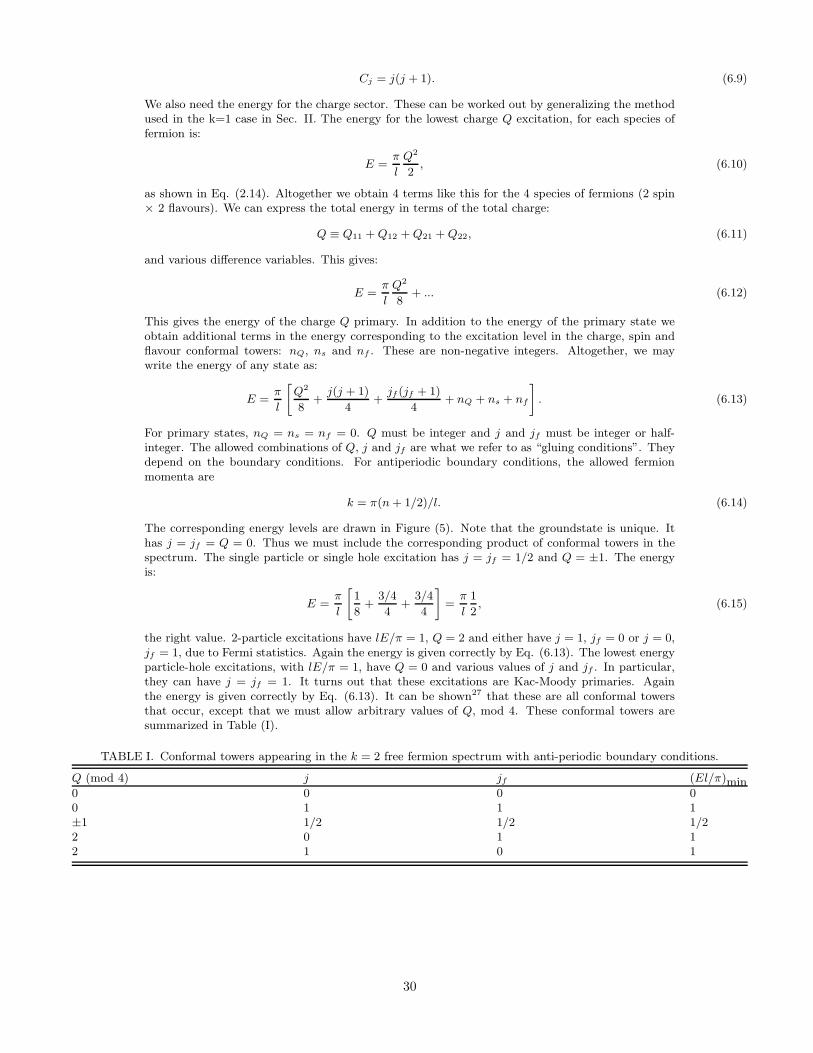
the right value. 2-particle excitations have lE/π = 1, Q = 2 and either have j = 1, jf = 0 or j = 0,jf = 1, due to Fermi statistics. Again the energy is given correctly by Eq. (6.13). The lowest energyparticle-hole excitations, with lE/π = 1, have Q = 0 and various values of j and jf . In particular,they can have j = jf = 1. It turns out that these excitations are Kac-Moody primaries. Againthe energy is given correctly by Eq. (6.13). It can be shown27 that these are all conformal towersthat occur, except that we must allow arbitrary values of Q, mod 4. These conformal towers aresummarized in Table (I).

TABLE I. Conformal towers appearing in the k = 2 free fermion spectrum with anti-periodic boundary conditions.

Q (mod 4) j jf (El/π)min0 0 0 00 1 1 1±1 1/2 1/2 1/22 0 1 12 1 0 1

30

Now consider fusion with the j = 1 primary. This has the effect of shuffling the spin conformaltowers in the following way:

0 → 1

1/2 → 1/2

1 → 0. (6.16)

The spectrum of Table (I) goes into that of Table (II) under this shuffling. It can be checked thatthis corresponds to free fermions with a π/2 phase shift, i.e. periodic boundary conditions, or a shiftof the Fermi energy by 1/2 a level spacing, drawn in Figure (6). Now note that the groundstateis 24 = 16-fold degenerate, since the zero-energy level may be filled or empty for each species offermion. The charge , Q, in Table (II) is now measured relative to the symmetric case where 2 ofthese levels are filled and 2 are empty. Also note that if make the replacement:

Q→ Q− 2, (6.17)

we get back the previous spectrum of Table (I). Making this replacement in Eq. (6.13), we obtain:

El

π→ El

π+Q

2(6.18)

(ignoring a constant). This corresponds to shifting the Fermi energy by 1/2-spacing; i.e. a π/2phase shift.

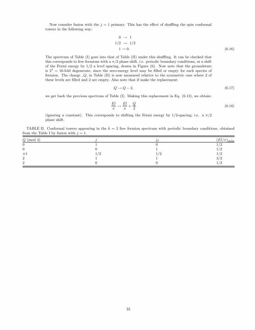
TABLE II. Conformal towers appearing in the k = 2 free fermion spectrum with periodic boundary conditions, obtainedfrom the Table I by fusion with j = 1.

Q (mod 4) j jf (El/π)min0 1 0 1/20 0 1 1/2±1 1/2 1/2 1/22 1 1 3/22 0 0 1/2

31

In the overscreened case the fusion rules are more interesting. They lead to spectra which cannotbe obtained by applying any simple linear boundary conditions to the free fermions. Thus we mayrefer to these as non-Fermi liquid fixed points. It might be possible to find some kind of non-lineardescription of the boundary conditions in this case. But note that a non-linear boundary condi-tion effectively introduces an interaction into the theory at the boundary. A boundary conditionquadratic in the fermion fields might induce an additional condition quartic in fields, etc. Thusspecification of non-linear boundary conditions could be very difficult. Cardy’s formalism cleverlysidesteps this problem by the device of focussing on the boundary states instead of boundary condi-tions, and providing a method (fusion) for producing these boundary states. As was stated above,and we will continue to see in what follows, knowledge of the boundary states will determine allphysical properties of the theory so nothing is lost by using this abstract description of the boundarycondition.

For the k = 2, s = 1/2 example, the fusion rules give:

0 → 1/2

1/2 → 0 ⊕ 1

1 → 1/2. (6.19)

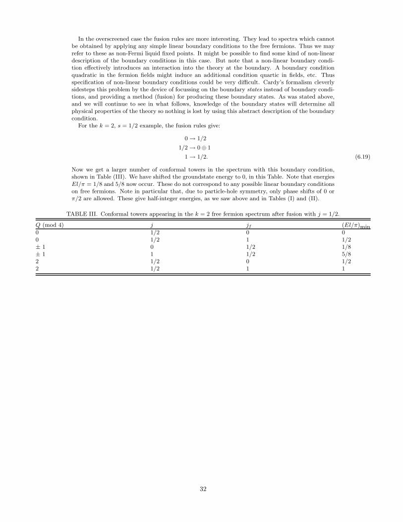
Now we get a larger number of conformal towers in the spectrum with this boundary condition,shown in Table (III). We have shifted the groundstate energy to 0, in this Table. Note that energiesEl/π = 1/8 and 5/8 now occur. These do not correspond to any possible linear boundary conditionson free fermions. Note in particular that, due to particle-hole symmetry, only phase shifts of 0 orπ/2 are allowed. These give half-integer energies, as we saw above and in Tables (I) and (II).

TABLE III. Conformal towers appearing in the k = 2 free fermion spectrum after fusion with j = 1/2.

Q (mod 4) j jf (El/π)min0 1/2 0 00 1/2 1 1/2± 1 0 1/2 1/8± 1 1 1/2 5/82 1/2 0 1/22 1/2 1 1

32

This spectrum was compared with numerical work on the k = 2, s = 1/2 Kondo effect andthe agreement was excellent (to within 5% for several of the lowest energy states).14 This providesevidence that the fusion rule hypothesis is correct in the overscreened case.

B. Impurity Entropy

We define the impurity entropy as:

Simp(T ) ≡ liml→∞[S(l, T ) − S0(l, T )], (6.20)

where S0(l, T ) is the free fermion entropy, proportional to l, in the absence of the impurity. Wewill find an interesting, non-zero value for Simp(0). Note that, for zero Kondo coupling, Simp =

ln[s(s + 1)], simply reflecting the groundstate degeneracy of the free spin. In the case of exactscreening, (k = 2s), Simp(0) = 0. For underscreening,

Simp(0) = ln[s′(s′ + 1)], (6.21)

where s′ ≡ s − k/2. What happens for overscreening? Surprisingly, we will obtain, in general, thelog of a non-integer, implying a sort of “non-integer groundstate degeneracy”.

To proceed, we show how to calculate Simp(0) from the boundary state. All calculations are

done in the scaling limit, ignoring irrelevant operators, so that Simp(T ) is a constant, independentof T , and characterizing the particular boundary condition. It is important, however, that we takethe limit l → ∞ first, as specified in Eq. (6.20), at fixed, non-zero T . i.e. we are interested in thelimit, l/β → ∞. Thus it is convenient to use the first expression for the partition function, ZAB inEq. (5.7):

ZAB =∑

a

< A|a0 >< a0|B > χa(e−4πl/β) → eπlc/6β < A|00 >< 00|B > . (6.22)

Here |00 > labels the groundstate in the conformal tower of the identity operator. c is the conformalanomaly. Thus the free energy is:

FAB = −πcT 2l/6 − T ln < A|00 >< 00|B > . (6.23)

The first term gives the specific heat:

C = πcT l/3 (6.24)

and the second gives the impurity entropy:

Simp = ln < A|00 >< 00|B > . (6.25)

This is a sum of contributions from the two boundaries,

Simp = SA + SB. (6.26)

Thus we see that the “groundstate degeneracy” gA, associated with boundary condition A is:

exp[SimpA] =< A|00 >≡ gA. (6.27)

Here we have used our freedom to choose the phase of the boundary state so that gA > 0. Forour original, anti-periodic, boundary condition, g = 0. For the Kondo problem we expect the lowT impurity entropy to be given by the value at the infrared fixed point. Since this is obtained byfusion with the spin-s (or k/2) operator, we obtain from Eq. (5.26),

g =S0

s

S00

. (6.28)

The modular S-matrix for SU(2)k is:27,30

Sjj′(k) =

√

2

2 + ksin

[

π(2j + 1)(2j′ + 1)

2 + k

]

, (6.29)

so

33

g(s, k) =sin[π(2s+ 1)/(2 + k)]

sin[π/(2 + k)]. (6.30)

This formula agrees exactly with the Bethe ansatz result.36 This formula has various interestingproperties. Recall that in the case of exact or underscreening (s ≥ k/2) we must replace s by k/2 inthis formula, in which case it reduces to 1. Thus the groundstate degeneracy is 1 for exact screening.For underscreening we must multiply g by (2s′ +1) to account for the decoupled, partially screenedimpurity. Note that, in the overscreened case, where s < k/2, we have:

1

2 + k<

2s+ 1

2 + k< 1 − 1

2 + k, (6.31)

so g > 1. In the case k → ∞ with s held fixed, g → 2s + 1, i.e. the entropy of the impurity spinis hardly reduced at all by the Kondo interaction, corresponding to the fact that the critical pointoccurs at weak coupling. In general, for underscreening:

1 < g < 2s + 1. (6.32)

i.e. the free spin entropy is somewhat reduced, but not completely eliminated. Furthermore, g isnot, in general, an integer. For instance, for k = 2 and s = 1/2, g =

√2. Thus we may say that

there is a non-integer “groundstate degeneracy”. Note that in all cases the groundstate degeneracy isreduced under renormalization from the zero Kondo coupling fixed point to the infrared stable fixedpoint. This is a special case of what we believe to be a general result: the groundstate degeneracy

always decreases under renormalization. This appears to be related to Zamolodchikov’s c-theorem37

which states that the conformal anomaly parameter, c, always decreases under renormalization.The intuitive explanation of the c-theorem is that, as we probe lower energy scales, degrees offreedom which appeared approximately massless start to exhibit a mass. This freezes out theircontribution to the specific heat, the slope of which can be taken as the definition of c. In the caseof the “g-theorem” the intuitive explanation is that, as we probe lower energy scales, approximatelydegenerate levels of impurities exhibit small splittings, reducing the degeneracy.

So far, only a perturbative proof of the g-theorem has been given.15 It is completely analogous to aperturbative proof of the c-theorem given by Cardy and Ludwig,38 independently of Zamolodchikov’smore general proof. For the g-theorem proof, we consider perturbing around a boundary CFT fixedpoint with a barely relevant boundary operator. i.e. the action is:

S = S0 − λ

∫ β

0

dτφ(0, τ ), (6.33)

where φ has dimension 1 − y with 0 < y << 1. The β-function has the form:

β = yλ− bλ2, (6.34)

for some constant, b. There is a nearby fixed point at:

λc = y/b. (6.35)

It is possible to calculate the small change in g using renormalization group improved perturbationtheory. This gives:

δg/g = −π2y3/3b2 < 0. (6.36)

C. Boundary Green’s Functions: Two-Point Functions, T=0 Resistivity

In this sub-section we explain the basic concepts for calculation of Green’s functions in the presenceof a conformally invariant boundary condition.35 We then work out the case of two-point funtionsin detail. Finally we show how this gives information about the Kondo problem.

The most important point is the consequence of the identification of left and right-moving sectors,discussed in Sec. V. In general, in the bulk theory, a typical local operator is a product of left andright-moving factors:

φ(x) = φL(x)φR(x). (6.37)

34

Here x is the spatial co-ordinate; we suppress the time-dependence. However, in the presence of aboundary, we use:

φR(x) = φL(−x). (6.38)

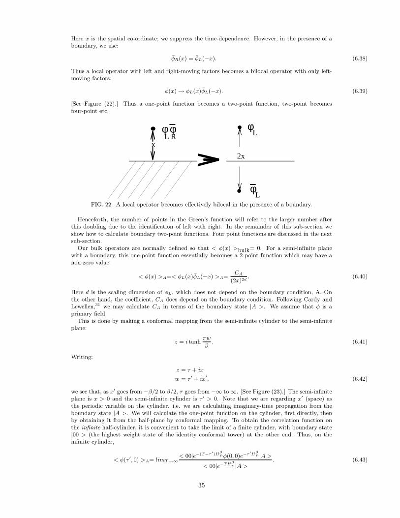
Thus a local operator with left and right-moving factors becomes a bilocal operator with only left-moving factors:

φ(x) → φL(x)φL(−x). (6.39)

[See Figure (22).] Thus a one-point function becomes a two-point function, two-point becomesfour-point etc.

2x

Rφ

LL

φ

x

L

φ φ

FIG. 22. A local operator becomes effectively bilocal in the presence of a boundary.

Henceforth, the number of points in the Green’s function will refer to the larger number afterthis doubling due to the identification of left with right. In the remainder of this sub-section weshow how to calculate boundary two-point functions. Four point functions are discussed in the nextsub-section.

Our bulk operators are normally defined so that < φ(x) >bulk= 0. For a semi-infinite planewith a boundary, this one-point function essentially becomes a 2-point function which may have anon-zero value:

< φ(x) >A=< φL(x)φL(−x) >A=CA

(2x)2d. (6.40)

Here d is the scaling dimension of φL, which does not depend on the boundary condition, A. Onthe other hand, the coefficient, CA does depend on the boundary condition. Following Cardy andLewellen,31 we may calculate CA in terms of the boundary state |A >. We assume that φ is aprimary field.

This is done by making a conformal mapping from the semi-infinite cylinder to the semi-infiniteplane:

z = i tanhπw

β. (6.41)

Writing:

z = τ + ix

w = τ ′ + ix′, (6.42)

we see that, as x′ goes from −β/2 to β/2, τ goes from −∞ to ∞. [See Figure (23).] The semi-infiniteplane is x > 0 and the semi-infinite cylinder is τ ′ > 0. Note that we are regarding x′ (space) asthe periodic variable on the cylinder. i.e. we are calculating imaginary-time propagation from theboundary state |A >. We will calculate the one-point function on the cylinder, first directly, thenby obtaining it from the half-plane by conformal mapping. To obtain the correlation function onthe infinite half-cylinder, it is convenient to take the limit of a finite cylinder, with boundary state|00 > (the highest weight state of the identity conformal tower) at the other end. Thus, on theinfinite cylinder,

< φ(τ ′, 0) >A= limT→∞< 00|e−(T−τ ′)H

β

P φ(0, 0)e−τ ′Hβ

P |A >

< 00|e−THβ

P |A >. (6.43)

35

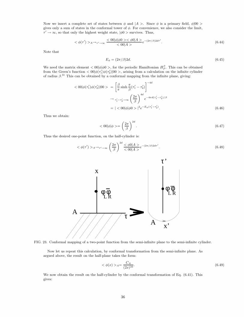
Now we insert a complete set of states between φ and |A >. Since φ is a primary field, φ|00 >gives only a sum of states in the conformal tower of φ. For convenience, we also consider the limit,τ ′ → ∞, so that only the highest weight state, |φ0 > survives. Thus,

< φ(τ ′) >A→τ ′→∞< 00|φ|φ0 >< φ0|A >

< 00|A >e−(2π/β)2dτ ′

. (6.44)

Note that

Eφ = (2π/β)2d. (6.45)

We need the matrix element < 00|φ|φ0 >, for the periodic Hamiltonian HβP . This can be obtained

from the Green’s function < 00|φ(τ ′1)φ(τ ′2)|00 >, arising from a calculation on the infinite cylinderof radius β.31 This can be obtained by a conformal mapping from the infinite plane, giving:

< 00|φ(τ ′1)φ(τ ′2)|00 > =

[

β

πsinh

π

β(τ ′1 − τ ′2)

]−4d

→ τ ′1−τ ′

2→∞

(

2π

β

)4d

e−4πd(τ ′1−τ ′

2)/β

= | < 00|φ|φ0 > |2e−Eφ(τ ′1−τ ′

2). (6.46)

Thus we obtain:

< 00|φ|φ >=

(

2π

β

)2d

. (6.47)

Thus the desired one-point function, on the half-cylinder is:

< φ(τ ′) >A→τ ′→∞

(

2π

β

)2d< φ0|A >

< 00|A >e−(2π/β)2dτ ′

. (6.48)

A

xτ ’

x’τ

RLφ φ RL

φ φ

A

FIG. 23. Conformal mapping of a two-point function from the semi-infinite plane to the semi-infinite cylinder.

Now let us repeat this calculation, by conformal transformation from the semi-infinite plane. Asargued above, the result on the half-plane takes the form:

< φ(x) >A=CA

(2x)2d. (6.49)

We now obtain the result on the half-cylinder by the conformal transformation of Eq. (6.41). Thisgives:

36

< φ(τ ) >1/2-cylinderA = | dz

dw|2d < φ(x) >

planeA

=

(

π

βsech2 πτ

′

β

)2dCA

(2x)2d

= CA

(

π

β

sech2πτ ′/β

2 tanh πτ ′/β

)2d

→ CA

(

2π

βe−2πτ ′/β

)2d

. (6.50)

Thus, equating Eq. (6.48) and (6.50), we finally obtain the desired formula for the coefficient CA,defined in Eq. (6.40):

CA =< φ0|A >

< 00|A >. (6.51)

If |A > is obtained by fusion with primary operator c from some reference state |F > (standing forfree), then:

CA = CfreeA

Sφc /S

φ0

S0c/S0

0

. (6.52)

Eq. (6.40) can be immediately generalized to the case where the left and right factors occur atdifferent points in the upper half-plane:

< φL(z)φR(z′) >A=CA

[(τ − τ ′) + i(x+ x′)]2d. (6.53)

An important application of this formula in the Kondo problem is to the single fermion Green’sfunction, < ψL(z)†ψR(z′) >. In the case of periodic boundary conditions:

< ψ†iαL (x)ψRjβ(x) >free = < ψ†iα

L (x)ψLjβ(−x) >

=δi

jδαβ

2x. (6.54)

We may obtain the one-point function at the Kondo fixed point by fusion. The fermion operatorcan be written as a product of spin flavour and charge operators:

ψLjα ∝ gαhjei√

2π/kφ. (6.55)

Here g and h are the left moving factors of the primary fields of the WZW models, transformingunder the fundamental representation. i.e. g has s=1/2. We may use Eq. (6.52). The Kondoboundary condition is obtained by fusion with the spin-s conformal tower, where s is the spin of theimpurity. Thus:

< ψ†iαL (x)ψRjβ(x) >Kondo

s =δi

jδαβ

2x

S1/2s /S

1/20

S0s/S0

0

=cos[π(2s+ 1)/(2 + k)]

cos[π/(2 + k)]

δijδ

αβ

2x(6.56)

Here we have used the SU(2) modular S-matrix given in Eq. (6.30) . There are several interestingpoints to notice about this formula. First of all, we see that for the case of exact or underscreening,where s = k/2, the cosine in the numerator in Eq. (6.56) becomes:

cos π(k + 1)/(k + 2) = − cosπ/(k + 2). (6.57)

Thus:

< ψ†LψR >Kondo

k/2 = − < ψ†LψR >free . (6.58)

As expected, this corresponds to a π/2 phase shift:

ψR(0) = e2iδψL(0) = −ψL(0). (6.59)

37

In general, we may define a one-particle into one-particle S-matrix element , S(1) by:

< ψ†LψR >= S(1) < ψ†

LψR >free, (6.60)

with:

S(1) =cos[π(2s+ 1)/(2 + k)]

cos[π/(2 + k)]. (6.61)

We see that in the overscreened case, |S(1)| < 1. S(1) is the matrix element, at the Fermi energy,for a single electron to scatter off the impurity into a single electron. In the case where |S(1)| = 1,we see, by unitarity, that there is zero probability for a single electron to scatter into anything buta single electron at the Fermi energy, at zero temperature. This is precisely the starting point forLandau’s Fermi liquid theory. Thus we refer to such cases as Fermi liquid boundary conditions. Inthe overscreened case, where |S(1)| < 1, this inelastic scattering probability is non-zero so we havenon-Fermi liquid boundary conditions. It is interesting to note that in the large k limit (with s heldfixed), S(1) → 1, corresponding to the fixed point occuring at weak coupling. We also note that,for k = 2, s = 1/2, S(1) = 0. This is related to the symmetry between the zero coupling (S(1) = 1)and infinite coupling (S(1) = −1) fixed point, mentioned above. In this case the one particle to oneparticle scattering rate vanishes!

From the electron self-energy we can obtain the lifetime and hence the resistivity for a dilutearray of impurities by the Kubo formula15 giving a T = 0 resistivity:

ρ(0) =3ni

kπ(eνvF )2

[

1 − S(1)

2

]

. (6.62)

Here ni is the impurity density. The first factor is the “unitary limit”. i.e. this is the largest possibleresistivity that can occur for a dilute array of non-magnetic impurities. It is only realised in theKondo problem in the Fermi liquid case (exact or overscreened). Otherwise the resistivity is reduced

by the factor[

1−S(1)

2

]

, which goes to zero for large k.

D. Four Point Boundary Green’s Functions, Spin-Density Green’s Function

In this sub-section we sketch how four-point functions of chiral operators (or two-point functionsof non-chiral ones) are calculated in the presence of a boundary, using the particular example ofthe fermion four-point function with the Kondo boundary condition. For more details, see Ref. (16). Similarly to the case of the two-point function, we will find that the four-point function isdetermined by bulk properties up to a constant which can be expressed in terms of matrix elementsinvolving the boundary state.

We consider the Green’s function:

G ≡< ψLαi(z1)ψ†βjL (z2)ψRβj(z3)ψ

†αiR (z4) > . (6.63)

We suppress spin and flavour indices in what follows, but it must be understood that we are dealingwith tensors throughout. The first step is to regard the right-moving fields as reflected left-movingones:

ψR(z) → ψL(z∗). (6.64)

Then we use Eq. (6.55) to express G as a product of charge, spin and flavour Green’s functions:

G = GcGsGf . (6.65)

The form of Gc is unique up to a multiplicative constant, and is unaffected by the boundary. Gs

and Gf are partially determined by the bulk conformal field theories. i.e. they must be solutions ofthe linear Knizhnik-Zamolodchikov (KZ) equations.26 These equations have two solutions in bothcases. We label them Gs(p) and Gf (q) where p and q take values 0 and 1. They are tensors in spinand flavour space; we suppress these indices. Thus we may schematically write the solution as :

G =

1∑

p,q=0

ap,qGcGs(p)Gf (q). (6.66)

38

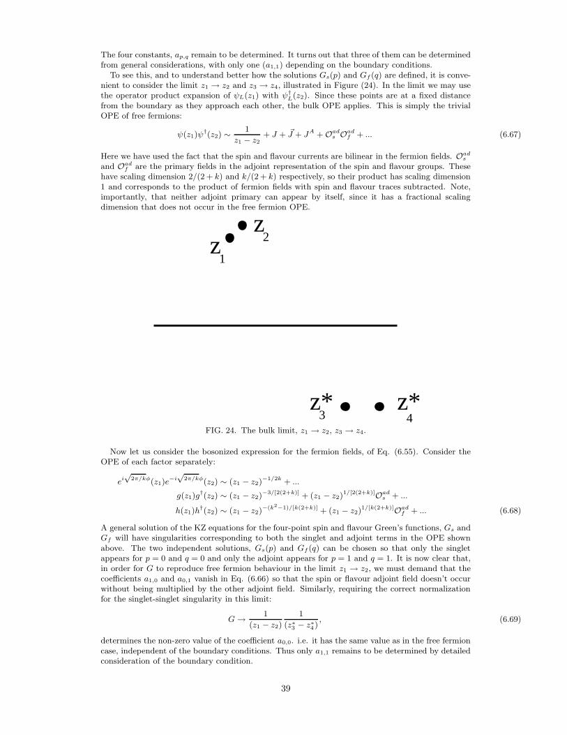
The four constants, ap,q remain to be determined. It turns out that three of them can be determinedfrom general considerations, with only one (a1,1) depending on the boundary conditions.

To see this, and to understand better how the solutions Gs(p) and Gf (q) are defined, it is conve-nient to consider the limit z1 → z2 and z3 → z4, illustrated in Figure (24). In the limit we may usethe operator product expansion of ψL(z1) with ψ†

L(z2). Since these points are at a fixed distancefrom the boundary as they approach each other, the bulk OPE applies. This is simply the trivialOPE of free fermions:

ψ(z1)ψ†(z2) ∼ 1

z1 − z2+ J + ~J + JA + Oad

s Oadf + ... (6.67)

Here we have used the fact that the spin and flavour currents are bilinear in the fermion fields. Oads

and Oadf are the primary fields in the adjoint representation of the spin and flavour groups. These

have scaling dimension 2/(2 + k) and k/(2 + k) respectively, so their product has scaling dimension1 and corresponds to the product of fermion fields with spin and flavour traces subtracted. Note,importantly, that neither adjoint primary can appear by itself, since it has a fractional scalingdimension that does not occur in the free fermion OPE.

z1

4

z2

z* z*3

FIG. 24. The bulk limit, z1 → z2, z3 → z4.

Now let us consider the bosonized expression for the fermion fields, of Eq. (6.55). Consider theOPE of each factor separately:

ei√

2π/kφ(z1)e−i√

2π/kφ(z2) ∼ (z1 − z2)−1/2k + ...

g(z1)g†(z2) ∼ (z1 − z2)

−3/[2(2+k)] + (z1 − z2)1/[2(2+k)]Oad

s + ...

h(z1)h†(z2) ∼ (z1 − z2)

−(k2−1)/[k(2+k)] + (z1 − z2)1/[k(2+k)]Oad

f + ... (6.68)

A general solution of the KZ equations for the four-point spin and flavour Green’s functions, Gs andGf will have singularities corresponding to both the singlet and adjoint terms in the OPE shownabove. The two independent solutions, Gs(p) and Gf (q) can be chosen so that only the singletappears for p = 0 and q = 0 and only the adjoint appears for p = 1 and q = 1. It is now clear that,in order for G to reproduce free fermion behaviour in the limit z1 → z2, we must demand that thecoefficients a1,0 and a0,1 vanish in Eq. (6.66) so that the spin or flavour adjoint field doesn’t occurwithout being multiplied by the other adjoint field. Similarly, requiring the correct normalizationfor the singlet-singlet singularity in this limit:

G→ 1

(z1 − z2)

1

(z∗3 − z∗4), (6.69)

determines the non-zero value of the coefficient a0,0. i.e. it has the same value as in the free fermioncase, independent of the boundary conditions. Thus only a1,1 remains to be determined by detailedconsideration of the boundary condition.

39

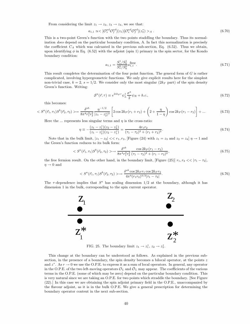
From considering the limit z1 → z2, z3 → z4, we see that:

a1,1 ∝< [Oads Oad

f ](z1)[Oads Oad

f ](z∗3) >A . (6.70)

This is a two-point Green’s function with the two points staddling the boundary. Thus its normal-ization does depend on the particular boundary condition, A. In fact this normalization is preciselythe coefficient CA which was calcuated in the previous sub-section, Eq. (6.52). Thus we obtain,upon identifying φ in Eq. (6.52) with the adjoint (spin 1) primary in the spin sector, for the Kondoboundary condition:

a1,1 =S1

s/S10

S0s/S0

0

afree1,1 . (6.71)

This result completes the determination of the four point function. The general form of G is rathercomplicated, involving hypergeometric functions. We only give explicit results here for the simplestnon-trivial case, k = 2, s = 1/2. We consider only the most singular (2kF part) of the spin densityGreen’s function. Writing:

Sa(~r, τ ) ≡ e2ikF rψ†L

σa

2ψR + h.c., (6.72)

this becomes:

< Sa(~r1, τ1)Sb(~r2, τ2) >=

δab

8π4r21r22

η−1/2

|z1 − z∗2 |2[

2 cos 2kF (r1 + r2) +

(

2 +η

1 − η

)

cos 2kF (r1 − r2)

]

+ ... (6.73)

Here the ... represents less singular terms and η is the cross-ratio:

η ≡ − (z1 − z∗1)(z2 − z∗2)

(z1 − z∗2)(z2 − z∗1)=

4r1r2(τ1 − τ2)2 + (r1 + r2)2

. (6.74)

Note that in the bulk limit, |z1 − z2| << r1, r2, [Figure (24) with z1 = z3 and z2 = z4] η → 1 andthe Green’s function reduces to its bulk form:

< Sa(~r1, τ1)Sb(~r2, τ2) >→ δab

8π4r21r22

cos 2kF (r1 − r2)

(τ1 − τ2)2 + (r1 − r2)2, (6.75)

the free fermion result. On the other hand, in the boundary limit, [Figure (25)] r1, r2 << |τ1 − τ2|,η → 0 and

< Sa(~r1, τ1)Sb(~r2, τ2) >→ δab cos 2kF r1 cos 2kF r2

4π4(r1r2)3/2|τ1 − τ2|. (6.76)

The τ -dependence implies that Sa has scaling dimension 1/2 at the boundary, although it hasdimension 1 in the bulk, corresponding to the spin current operator.

z z

1

1

2

2

z* z*FIG. 25. The boundary limit z1 → z∗1 , z2 → z∗2 .

This change at the boundary can be understood as follows. As explained in the previous sub-section, in the presence of a boundary, the spin density becomes a bilocal operator, at the points zand z∗. As r → 0 we use the O.P.E. to express it as a sum of local operators. In general, any operatorin the O.P.E. of the two left-moving operators OL and OL may appear. The coefficients of the variousterms in the O.P.E. (some of which may be zero) depend on the particular boundary condition. Thisis very natural since we are taking an O.P.E. for two points which straddle the boundary. [See Figure(22).] In this case we are obtaining the spin adjoint primary field in the O.P.E., unaccompanied bythe flavour adjoint, as it is in the bulk O.P.E. We give a general prescription for determining theboundary operator content in the next sub-section.

40

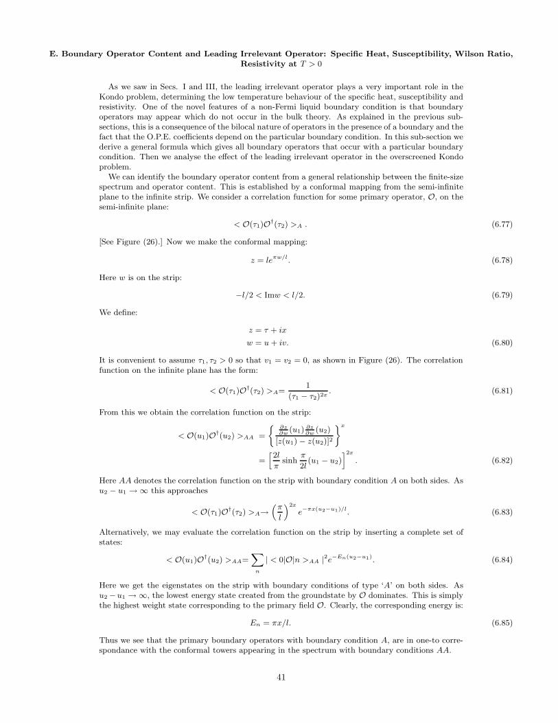
E. Boundary Operator Content and Leading Irrelevant Operator: Specific Heat, Susceptibility, Wilson Ratio,

Resistivity at T > 0

As we saw in Secs. I and III, the leading irrelevant operator plays a very important role in theKondo problem, determining the low temperature behaviour of the specific heat, susceptibility andresistivity. One of the novel features of a non-Fermi liquid boundary condition is that boundaryoperators may appear which do not occur in the bulk theory. As explained in the previous sub-sections, this is a consequence of the bilocal nature of operators in the presence of a boundary and thefact that the O.P.E. coefficients depend on the particular boundary condition. In this sub-section wederive a general formula which gives all boundary operators that occur with a particular boundarycondition. Then we analyse the effect of the leading irrelevant operator in the overscreened Kondoproblem.

We can identify the boundary operator content from a general relationship between the finite-sizespectrum and operator content. This is established by a conformal mapping from the semi-infiniteplane to the infinite strip. We consider a correlation function for some primary operator, O, on thesemi-infinite plane:

< O(τ1)O†(τ2) >A . (6.77)

[See Figure (26).] Now we make the conformal mapping:

z = leπw/l. (6.78)

Here w is on the strip:

−l/2 < Imw < l/2. (6.79)

We define:

z = τ + ix

w = u+ iv. (6.80)

It is convenient to assume τ1, τ2 > 0 so that v1 = v2 = 0, as shown in Figure (26). The correlationfunction on the infinite plane has the form:

< O(τ1)O†(τ2) >A=1

(τ1 − τ2)2x. (6.81)

From this we obtain the correlation function on the strip:

< O(u1)O†(u2) >AA =

{

∂z∂w

(u1)∂z∂w

(u2)

[z(u1) − z(u2)]2

}x

=[

2l

πsinh

π

2l(u1 − u2)

]2x

. (6.82)

Here AA denotes the correlation function on the strip with boundary condition A on both sides. Asu2 − u1 → ∞ this approaches

< O(τ1)O†(τ2) >A→(

π

l

)2x

e−πx(u2−u1)/l. (6.83)

Alternatively, we may evaluate the correlation function on the strip by inserting a complete set ofstates:

< O(u1)O†(u2) >AA=∑

n

| < 0|O|n >AA |2e−En(u2−u1). (6.84)

Here we get the eigenstates on the strip with boundary conditions of type ‘A’ on both sides. Asu2 −u1 → ∞, the lowest energy state created from the groundstate by O dominates. This is simplythe highest weight state corresponding to the primary field O. Clearly, the corresponding energy is:

En = πx/l. (6.85)

Thus we see that the primary boundary operators with boundary condition A, are in one-to corre-spondance with the conformal towers appearing in the spectrum with boundary conditions AA.

41

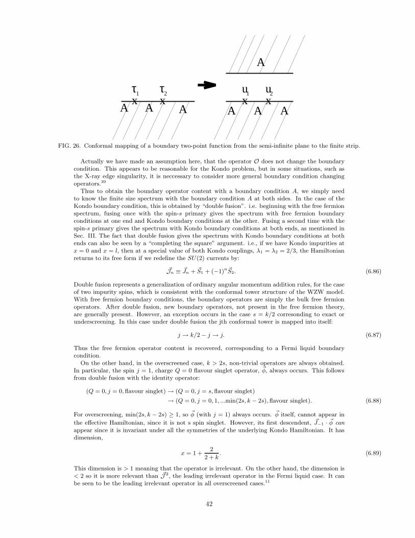
2

x xA A A A A A

A

x xτ τ u u1 12

FIG. 26. Conformal mapping of a boundary two-point function from the semi-infinite plane to the finite strip.

Actually we have made an assumption here, that the operator O does not change the boundarycondition. This appears to be reasonable for the Kondo problem, but in some situations, such asthe X-ray edge singularity, it is neccessary to consider more general boundary condition changingoperators.39

Thus to obtain the boundary operator content with a boundary condition A, we simply needto know the finite size spectrum with the boundary condition A at both sides. In the case of theKondo boundary condition, this is obtained by “double fusion”. i.e. beginning with the free fermionspectrum, fusing once with the spin-s primary gives the spectrum with free fermion boundaryconditions at one end and Kondo boundary conditions at the other. Fusing a second time with thespin-s primary gives the spectrum with Kondo boundary conditions at both ends, as mentioned inSec. III. The fact that double fusion gives the spectrum with Kondo boundary conditions at bothends can also be seen by a “completing the square” argument. i.e., if we have Kondo impurities atx = 0 and x = l, then at a special value of both Kondo couplings, λ1 = λ2 = 2/3, the Hamiltonianreturns to its free form if we redefine the SU(2) currents by:

~Jn ≡ ~Jn + ~S1 + (−1)n~S2. (6.86)

Double fusion represents a generalization of ordinary angular momentum addition rules, for the caseof two impurity spins, which is consistent with the conformal tower structure of the WZW model.With free fermion boundary conditions, the boundary operators are simply the bulk free fermionoperators. After double fusion, new boundary operators, not present in the free fermion theory,are generally present. However, an exception occurs in the case s = k/2 corresonding to exact orunderscreening. In this case under double fusion the jth conformal tower is mapped into itself:

j → k/2 − j → j. (6.87)

Thus the free fermion operator content is recovered, corresponding to a Fermi liquid boundarycondition.

On the other hand, in the overscreened case, k > 2s, non-trivial operators are always obtained.In particular, the spin j = 1, charge Q = 0 flavour singlet operator, ~φ, always occurs. This followsfrom double fusion with the identity operator:

(Q = 0, j = 0,flavour singlet) → (Q = 0, j = s,flavour singlet)

→ (Q = 0, j = 0, 1, ...min(2s, k − 2s),flavour singlet). (6.88)

For overscreening, min(2s, k − 2s) ≥ 1, so ~φ (with j = 1) always occurs. ~φ itself, cannot appear in

the effective Hamiltonian, since it is not s spin singlet. However, its first descendent, ~J−1 · ~φ can

appear since it is invariant under all the symmetries of the underlying Kondo Hamiltonian. It hasdimension,

x = 1 +2

2 + k. (6.89)

This dimension is > 1 meaning that the operator is irrelevant. On the other hand, the dimension is< 2 so it is more relevant than ~J 2, the leading irrelevant operator in the Fermi liquid case. It canbe seen to be the leading irrelevant operator in all overscreened cases.11

42

We now discuss the calculation of various quantities to lowest non-vanishing order in the leadingirrelevant term in the effective Hamiltonian:

δH = λ1~J−1 · ~φ. (6.90)

We begin with the specific heat. The simple change of variables trick that we used in Sec. III for theFermi liquid case doesn’t work here. In fact, since ~J−1 · ~φ is a Virasoro primary operator (althougha Kac-Moody descendant) its one-point function continues to vanish even at finite temperature.Consequently, the leading contribution to the specific heat is second order in λ1. The contributionto the impurity free energy of O(λ2

1) is:

−βfimp =λ2

1

2

∫ β/2

−β/2

dτ1

∫ β/2

−β/2

dτ2T < ~J−1 · ~φ(τ1) ~J−1 · ~φ(τ2) > . (6.91)

Since ~J−1 · ~φ is a Virasoro primary, this two-point function is given by:

< ~J−1 · ~φ(τ1) ~J−1 · ~φ(τ2) > =3(2 + k/2)

|τ1 − τ2|2(1+∆)

→ 3(2 + k/2)

|βπ

sin πβ(τ1 − τ2)|2(1+∆)

. (6.92)

Here

∆ ≡ 2

2 + k, (6.93)

and we have assumed that ~φ has unit normalization:

< φa(τ1)φb(τ2) >=

δab

|τ1 − τ2|2∆. (6.94)

The normalization of ~J−1 · ~φ can then be fixed using the Kac-Moody algebra. A naive rescalingargument implies that:

fimp ∝ T 1+2∆. (6.95)

Actually the integral in Eq. (6.91) requires an ultraviolet cut-off. However, this only leads toadditional terms in fimp that vanish more rapidly as T → 0. Evaluating the universal term in Eq.

(6.91) explicitly, we obtain:

Cimp = −T∂2fimp

∂T 2= λ2

1

[

T 2∆π1+2∆(2∆)23(k

2+ 2)

1

2

Γ(1/2 − ∆)Γ(1/2)

Γ(1 − ∆)+O(T )

]

+O(λ31T

3∆) + ...

(for k > 2) (6.96)

Here Γ(x) is Euler’s Gamma function. Note that this result is independent of the magnitude of theimpurity spin, s. Also note that since, for k > 2, ∆ = 2/(2 + k) < 1/2, so the impurity specific heatis more singular than in the Fermi liquid case. In the particular case k = 2, where ∆ = 1/2, weobtain from Eq. (6.91):

Cimp = λ21π

29T ln(TK/T ) + ... (6.97)

Note that this is only more singular by a log than in the Fermi liquid case.The impurity susceptibility is also second order in λ1,

χimp ∝ βλ21

∫

dτ1dτ2dx1dx2 < ~J−1 · ~φ(τ1) ~J−1 · ~φ(τ2)J3(0, x1)J

3(0, x2) > . (6.98)

Again, by a scaling argument we see that:

χimp ∝ λ21T

2∆−1. (6.99)

By evaluating the integral in Eq. (6.98) explicitly, we can caluculate the Wilson ratio, RW for theoverscreened Kondo problem:

43

χimp

Cimp

Cbulkχbulk

≡ RW =(2 + k/2)(2 + k)2

18. (6.100)

We can calculate the Wilson ratio in the exactly screened, Fermi liquid, case, much more simply.In this case, the simple rescaling argument of Sec. III always works giving:

Cimp/Cs

χimp/χ= 1. (6.101)

Here Cs is the part of the bulk specific heat coming from the spin degrees of freedom. Hence theWilson ratio is given by

RW =C

Cs. (6.102)

It simply measures the ratio of the total bulk specific heat to that coming from the spin degrees offreedom. Using:

C =π

3cT, (6.103)

where c is the conformal anomaly, and the fact that c = 2k for 2k species of free fermions andc = 3k/(2 + k) for the level k SU(2) WZW model, we obtain:

RW =2(2 + k)

3, (6.104)

for the exactly screened Kondo problem.Finally we consider the T-dependence of the impurity resistivity. For more details, see Ref. ( 15).

We may write the electron Green’s function in the one-dimensional theory with the impurity at theorigin in the form:

G(r1,−r2, ωn) −G0(r1 + r2, ωn) = G0(r1, ωn)Σ1(ωn)G0(r2, ωn). (6.105)

In the three dimensional theory with a dilute random array of Kondo impurities, of density ni theself-energy becomes:

Σ3 =ni

νΣ1. (6.106)

The electron life-time is given by:

1

τ= −2ImΣR

3 , (6.107)

where the superscript R denotes the retarded Green’s function, obtained by analytic continuationfrom the Matsubara Green’s function. The conductivity is then expressed in terms of the lifetimein the standard way:

σ =2e2

3m2

∫

d3p

(2π)3

[

−dnF

dǫp

]

~p2τ (ǫp). (6.108)

Thus, we just need to calculate the one-dimensional self-energy, Σ1. This was already done, at T=0,in Subsection (VIC). There we showed that:

G = G0S(1), (6.109)

where S(1) is the scattering matrix element for 1-electron to go into 1-electron, given explicitly inEq. (6.61). This gave the resistivity:

ρ =1 − S(1)

2ρu, (6.110)

where ρu is the unitary limit resistivity. To obtain the leading T-dependence, we do perturbationtheory in the leading irrelevant coupling constant, λ1. In this case, there is a non-zero first ordercontribution:

δΣ1 ∝ λ1 < ψ ~J−1 · ~φψ† > . (6.111)

44

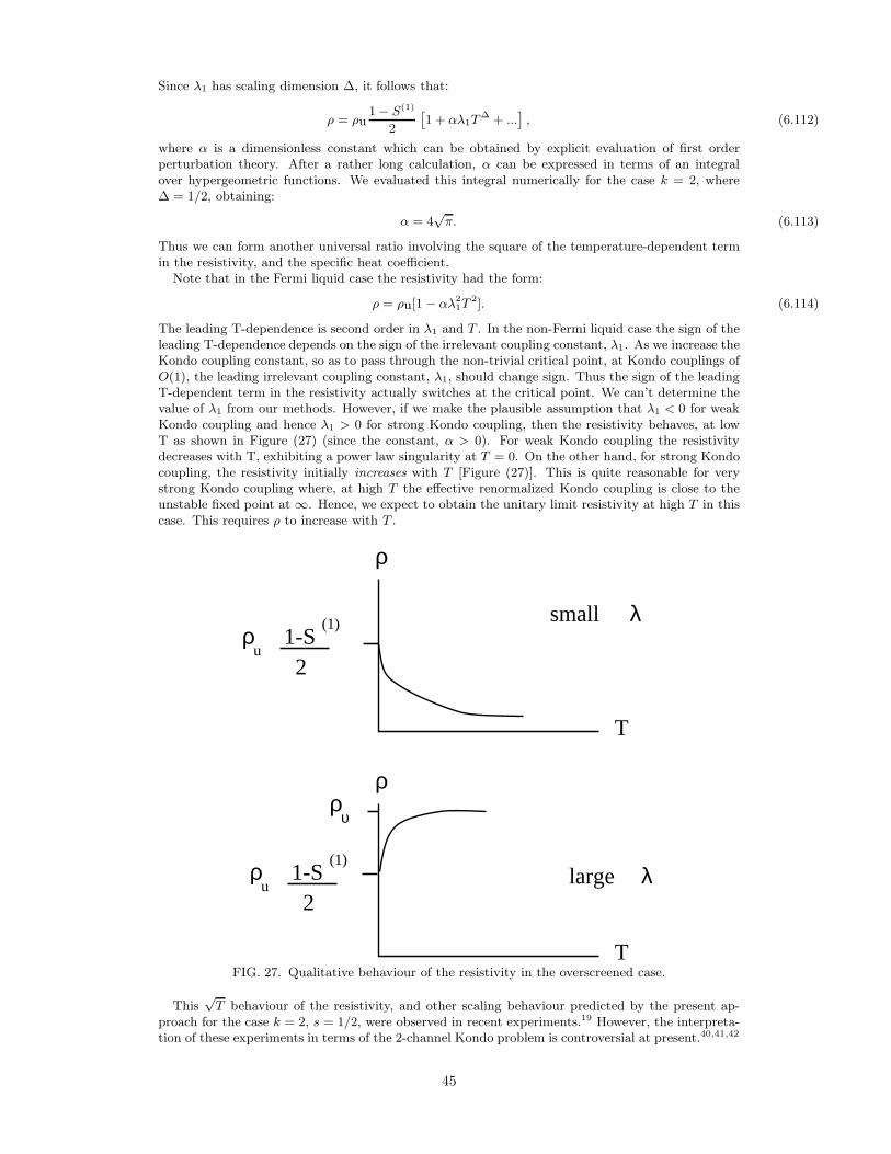
Since λ1 has scaling dimension ∆, it follows that:

ρ = ρu1 − S(1)

2

[

1 + αλ1T∆ + ...

]

, (6.112)

where α is a dimensionless constant which can be obtained by explicit evaluation of first orderperturbation theory. After a rather long calculation, α can be expressed in terms of an integralover hypergeometric functions. We evaluated this integral numerically for the case k = 2, where∆ = 1/2, obtaining:

α = 4√π. (6.113)

Thus we can form another universal ratio involving the square of the temperature-dependent termin the resistivity, and the specific heat coefficient.

Note that in the Fermi liquid case the resistivity had the form:

ρ = ρu[1 − αλ21T

2]. (6.114)

The leading T-dependence is second order in λ1 and T . In the non-Fermi liquid case the sign of theleading T-dependence depends on the sign of the irrelevant coupling constant, λ1. As we increase theKondo coupling constant, so as to pass through the non-trivial critical point, at Kondo couplings ofO(1), the leading irrelevant coupling constant, λ1, should change sign. Thus the sign of the leadingT-dependent term in the resistivity actually switches at the critical point. We can’t determine thevalue of λ1 from our methods. However, if we make the plausible assumption that λ1 < 0 for weakKondo coupling and hence λ1 > 0 for strong Kondo coupling, then the resistivity behaves, at lowT as shown in Figure (27) (since the constant, α > 0). For weak Kondo coupling the resistivitydecreases with T, exhibiting a power law singularity at T = 0. On the other hand, for strong Kondocoupling, the resistivity initially increases with T [Figure (27)]. This is quite reasonable for verystrong Kondo coupling where, at high T the effective renormalized Kondo coupling is close to theunstable fixed point at ∞. Hence, we expect to obtain the unitary limit resistivity at high T in thiscase. This requires ρ to increase with T .

υ

T

ρ

T

ρρ

u

small

large

λ

λ1-S2

(1)

ρ 1-S2

(1)

u

ρ

FIG. 27. Qualitative behaviour of the resistivity in the overscreened case.

This√T behaviour of the resistivity, and other scaling behaviour predicted by the present ap-

proach for the case k = 2, s = 1/2, were observed in recent experiments.19 However, the interpreta-tion of these experiments in terms of the 2-channel Kondo problem is controversial at present.40,41,42

45

ACKNOWLEDGMENTS

I would especially like to thank my main collaborator in this work, Andreas Ludwig. I wouldalso like to thank Chandra Varma for interesting me in this problem, Nathan Seiberg for suggestingthe “fusion rule hypothesis” and John Cardy and Dan Cox for their collaboration and helpfulsuggestions. I am very grateful to Ming Yu who produced a TEXversion, from my transparencies,of some lectures which I gave in Beijing in June, 1991. This essentially became Sections I-III. Thisresearch was supported in part by NSERC of Canada.

∗ Lectures given at the XXXVth Cracow School of Theoretical Physics, Zakopane, Poland, June, 1995. These lecture notesassume a certain familiarity with conformal field theory. Useful background information may be found in the lecture notesof Jean-Bernard Zuber in this series.

1 J. Kondo, Prog. Theor. Phys. 32, 37 (1964).2 P. Nozieres, Proc. of 14th Int. Conf. on Low Temp. Phys. [ Ed. M. Krusius and M. Vuorio ] V.5, P.339, (1975).3 K.G. Wilson, Rev. Mod. Phys. 47, 773 (1975).4 N. Andrei, Phys. Rev. Lett. 45, 379 (1980).5 P.B. Weigmann, Sov. Phys. J.E.T.P. Lett. 31, 392 (1980).6 P.W. Anderson, J. Phys. C3, 2346 (1970).7 P. Nozieres, J. Low Temp. Phys. 17, 31 (1974).8 P. Nozieres and A. Blandin, J. de Physique, 41, 193 (1980).9 I. Affleck, Nucl. Phys. B336, 517, 1990.

10 I. Affleck and A.W.W. Ludwig, Nucl. Phys. B352, 849(1991) .11 I. Affleck and A.W.W. Ludwig, Nucl. Phys. B360, 641(1991) .12 I. Affleck and A.W.W. Ludwig, Phys. Rev. Lett. 67, 161(1991) .13 A.W.W. Ludwig and I. Affleck, Phys. Rev, Lett. 67, 3160(1991) .14 I. Affleck, A.W.W. Ludwig, H-B. Pang and D. L. Cox, Phys. Rev. B45, 7918 (1992).15 I. Affleck and A.W.W. Ludwig, Phys. Rev. B48, 7297 (1993).16 A.W.W. Ludwig and I. Affleck, Nucl. Phys. B428, 545 (1994).17 I. Affleck and A.W.W. Ludwig, Phys. Rev. Lett. 68, 1046 (1992).18 I. Affleck, A.W.W. Ludwig and B.A. Jones, Phys. Rev. B52, 9528 (1995).19 D.C. Ralph, A.W.W. Ludwig, J. von Delft and R.A. Buhrman, Phys. Rev. Lett. 72, 1064 (1994).20 E. Wong and I. Affleck, Nucl. Phys. B417, 403 (1994).21 S. Eggert and I. Affleck, Phys. Rev. B46, 10866 (1992).22 E.S. Sørensen, S. Eggert and I. Affleck, J. Phys. A26, 6756 (1993).23 I. Affleck and J. Sagi, Nuc. Phys. B417, 374 (1994).24 D.L. Cox, Phys. Rev. Lett. 59, 1240 (1987).25 C. Sire, C.M. Varma, A.E. Ruckenstein and T. Giamarchi, Phys. Rev. Lett. 72, 2478 (1994).26 V.G. Knizhnik and A.B. Zamolodchikov, Nucl. Phys. B247, 83 (1984).27 D. Altschuler, M. Bauer and C. Itzykson, Comm. Math. Phys. 132, 349 (1990).28 J.L. Cardy, Nuc. Phys. B324, 581 (1989).29 N. Ishibashi, Mod. Phys. Lett. A4, 251 (1989); T. Onogi and N. Ishibashi, Nuc. Phys. B318, 239 (1989).30 V.G. Kac and M. Wakimoto, Adv. in Math. 70, 156 (1988).31 J.L. Cardy, Nucl. Phys. B270, 186 (1986).32 A.B. Zamolodchikov and V.A. Fateev, Sov. Jour. Nuc. Phys. 43, 657 (1986).33 D. Gepner and E. Witten, Nucl. Phys. B278, 493 (1986).34 E. Verlinde, Nucl. Phys. B300, 360 (1988).35 J.L. Cardy and D. Lewellen, Phys. Lett. B259, 274 (1991).36 A.M. Tsvelick, J. Phys. C18, 159 (1985).37 A.B. Zamolodchikov, Pis’ma Zh. Eksp. Teor. Fiz. 43, 565 (1986) [J.E.T.P. Lett. 43, 730 (1986)].38 A.W.W. Ludwig and J.L. Cardy, Nucl. Phys. B285, 687 (1987).39 I. Affleck and A.W.W. Ludwig, J. Phys. A27, 5375 (1994).40 N.S. Wingreen and B.L. Altshuler, Phys. Rev. Lett. 75, 769 (1995).41 D.C. Ralph, A.W.W. Ludwig, J. von Delft and R.A. Buhrman, Phys. Rev. Lett. 75, 770 (1995).42 A.L. Moustakas and D.S. Fisher, preprint cond-mat/9508011.

46