arXiv:alg-geom/9305002v1 3 May 1993
29
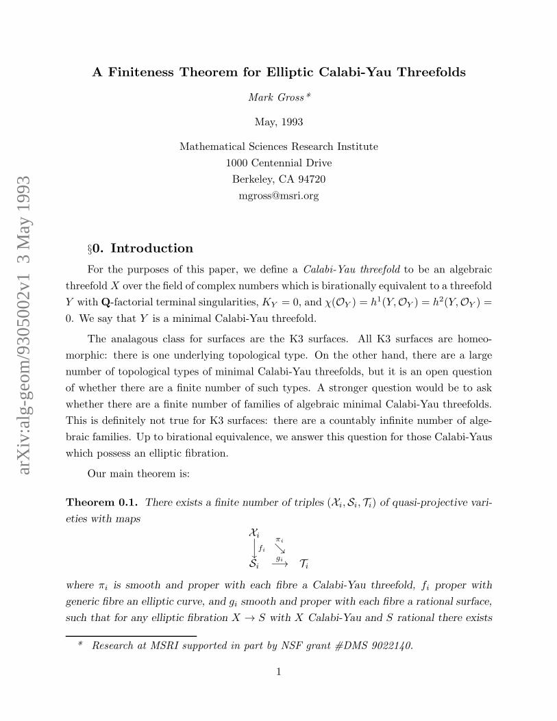
arXiv:alg-geom/9305002v1 3 May 1993 A Finiteness Theorem for Elliptic Calabi-Yau Threefolds Mark Gross* May, 1993 Mathematical Sciences Research Institute 1000 Centennial Drive Berkeley, CA 94720 [email protected] §0. Introduction For the purposes of this paper, we define a Calabi-Yau threefold to be an algebraic threefold X over the field of complex numbers which is birationally equivalent to a threefold Y with Q-factorial terminal singularities, K Y = 0, and χ(O Y )= h 1 (Y, O Y )= h 2 (Y, O Y )= 0. We say that Y is a minimal Calabi-Yau threefold. The analagous class for surfaces are the K3 surfaces. All K3 surfaces are homeo- morphic: there is one underlying topological type. On the other hand, there are a large number of topological types of minimal Calabi-Yau threefolds, but it is an open question of whether there are a finite number of such types. A stronger question would be to ask whether there are a finite number of families of algebraic minimal Calabi-Yau threefolds. This is definitely not true for K3 surfaces: there are a countably infinite number of alge- braic families. Up to birational equivalence, we answer this question for those Calabi-Yaus which possess an elliptic fibration. Our main theorem is: Theorem 0.1. There exists a finite number of triples (X i , S i , T i ) of quasi-projective vari- eties with maps X i f i π i ց S i g i −→ T i where π i is smooth and proper with each fibre a Calabi-Yau threefold, f i proper with generic fibre an elliptic curve, and g i smooth and proper with each fibre a rational surface, such that for any elliptic fibration X → S with X Calabi-Yau and S rational there exists * Research at MSRI supported in part by NSF grant #DMS 9022140. 1
Transcript of arXiv:alg-geom/9305002v1 3 May 1993
arX
iv:a
lg-g
eom
/930
5002
v1 3
May
199
3
A Finiteness Theorem for Elliptic Calabi-Yau Threefolds
Mark Gross*
May, 1993
Mathematical Sciences Research Institute
1000 Centennial Drive
Berkeley, CA 94720
§0. Introduction
For the purposes of this paper, we define a Calabi-Yau threefold to be an algebraic
threefoldX over the field of complex numbers which is birationally equivalent to a threefold
Y withQ-factorial terminal singularities, KY = 0, and χ(OY ) = h1(Y,OY ) = h2(Y,OY ) =
0. We say that Y is a minimal Calabi-Yau threefold.
The analagous class for surfaces are the K3 surfaces. All K3 surfaces are homeo-
morphic: there is one underlying topological type. On the other hand, there are a large
number of topological types of minimal Calabi-Yau threefolds, but it is an open question
of whether there are a finite number of such types. A stronger question would be to ask
whether there are a finite number of families of algebraic minimal Calabi-Yau threefolds.
This is definitely not true for K3 surfaces: there are a countably infinite number of alge-
braic families. Up to birational equivalence, we answer this question for those Calabi-Yaus
which possess an elliptic fibration.
Our main theorem is:
Theorem 0.1. There exists a finite number of triples (Xi,Si, Ti) of quasi-projective vari-
eties with maps
Xi
yfi
πi
ց
Sigi−→ Ti
where πi is smooth and proper with each fibre a Calabi-Yau threefold, fi proper with
generic fibre an elliptic curve, and gi smooth and proper with each fibre a rational surface,
such that for any elliptic fibration X → S with X Calabi-Yau and S rational there exists
* Research at MSRI supported in part by NSF grant #DMS 9022140.
1
a t ∈ Ti for some i such that there are birational maps X · · → (Xi)t, S · · → (Si)t with the
following diagram commutative:
X ·· → (Xi)t
y
y
S ·· → (Si)t
Let us make several remarks before indicating the idea of the proof. First, in this
theorem, we only consider elliptic fibrations with rational bases. If X is Calabi-Yau and
f : X → S an elliptic fibration, then S is either rational or birational to an Enriques
surface. In the latter case, X has a particularly simple structure. In particular, it is the
quotient of a three-fold Y with κ(Y ) = 0 and h1(OY ) > 0. (See Proposition 2.10).
Secondly, note that by [12], Theorem 1.2, we can thus obtain a finite number of fam-
ilies of minimal Calabi-Yau threefolds X ′i → Ti. However, because of the non-uniqueness
of minimal models for threefolds, not every minimal elliptic Calabi-Yau threefold will be
isomorphic to a (X ′i )t for some t ∈ Ti, but merely birational to such. It is not known if a
Calabi-Yau threefold always has a finite number of minimal models, even up to automor-
phism. Thus this result does not imply that there are only a finite number of topological
types of even non-singular minimal elliptic Calabi-Yau threefolds. Nevertheless, any such
threefold will be related by a series of flops to a finite number of possible topological types.
Thirdly, this result is a much stronger one than proved in [10], i.e. that there exists
a finite number of possible Euler characteristics of certain types of elliptic Calabi-Yau
threefolds. Our theorem says that there exists a complete, finite classification. One hopes
that any minimal Calabi-Yau threefold with sufficiently large Picard number is elliptic.
With our results, proving such a conjecture would then show that there are only a finite
number of types of minimal Calabi-Yau threefolds with Picard number greater than some
fixed number. This hopefully gives some suggestion that there are only a finite number of
types of algebraic Calabi-Yau threefolds.
If one were to ask how many families of elliptic Calabi-Yaus exist, the proof of this
theorem gives no hint, other than to suggest that it is a very large number. Making an
uninformed guess, I would conservatively expect thousands of families.
The proof of this theorem relies heavily on results about elliptic threefolds. Results
of [3] and [7] tell us how to go about classifying elliptic three-folds; we simply have to
apply them carefully. The proof also uses minimal model theory for threefolds, especially
as developed for elliptic threefolds in [4] and [6]. The main application of these techniques
is
2
Theorem 0.2. Let f : X → S be an elliptic fibration with X and S projective and
X having a minimal model with trivial canonical class. Then there exists a birationally
equivalent equidimensional fibration f : X → S where X is a minimal model of X and S
is a projective surface with only DuVal singularities.
Grassi in [4] has proven this theorem in the case that f has no multiple fibres. In fact,
in that case S can be found to be non-singular.
The second key ingredient is the calculation of the Tate-Shafarevich group for elliptic
fibrations in [3] and [7]. The most important fact is that the Tate-Shafarevich group is
finite for Calabi-Yau elliptic fibrations, something which fails for K3 surfaces. After these
two observations, most of the proof is simply careful bookkeeping to make sure that we
have not missed any threefolds.
I would like to thank M. Reid for suggesting this problem to me, and I. Dolgachev
and A. Grassi for many useful discussions.
§1. Generalities on Elliptic Threefolds.
We recall some basic definitions and state some general results about elliptic threefolds
which will be necessary. We note that all varieties in this paper are algebraic varieties of
finite type over the complex numbers.
Definition 1.1. A projective morphism f : X → S is called an elliptic fibration if its
generic fibre E is a regular curve of genus one and all fibres are geometrically connected.
f : X → S is called a model for E. The closed subset
Σred = Σred(f) = {s ∈ S|Xs is not regular}
is called the (reduced) discriminant locus. If t ∈ S is a codimension one point of S, then the
fibre type of t is the Kodaira fibre type (mIn, I∗n, II, II
∗, III, III∗, IV, IV ∗) of the central
fibre of a relatively minimal model (or Neron model) of X(t) = X ×S SpecOS,t. (OS,t is
the strict henselization of the local ring OS,t.) A collision is a singular point of Σ. The
closed subset
Σm = {s ∈ S|f is not smooth at any x ∈ f−1(s)}
is called the multiple locus of f . A fibre over a point s ∈ Σm is called multiple. A fibre is
called an isolated multiple fibre if it is over a zero-dimensional component of Σm. A section
(resp. a rational section) of f is a closed subscheme Y of X for which the restriction of f
to Y is an isomorphism (resp. a birational morphism).
Let f : X → S be an elliptic fibration between two non-singular complex varieties,
which is smooth off of a simple normal crossings divisor on S. Then by [11], Theorem
3
20, f∗ωX/S is an invertible sheaf. This defines a divisor on S, which we denote by ∆X/S
(or ∆ if no confusion will arise). If f : X → S is then just an elliptic fibration with X
and S having singularities in codimension 3 and 2 respectively, then there exists an open
subset S0 ⊆ S such that S − S0 is codimension 2 in S and if f0 is the induced morphism
X0 = X ×S S0 → S0, then X0 and S0 are non-singular and Σred(f0) has simple normal
crossings. Then ∆X0/S0is a Cartier divisor on S0, which extends to a Weil divisor on S,
which we denote by ∆X/S again.
Let {Mi} be the codimension one components of Σm, with fibre type miIa. We set
ΛX/S = ∆X/S +∑ mi − 1
miMi.
We then have
Lemma 1.2. Let f : X → S be an elliptic fibration with dimS = 2. Then there exists a
blow-up S′ → S and a birationally equivalent fibration f ′ : X ′ → S′ such that
1) f ′ is flat and relatively minimal, X ′ has only Q-factorial terminal singularities, S′ is
regular, and the reduced discriminant locus Σred of f ′ has simple normal crossings.
2) The modular function J gives a morphism J : S′ → P1, and ∆ = ∆X′/S′ is a divisor
on S′ such that
12∆ ∼ J∞ +∑
12aiDi
where J∞ is the fibre of J at∞ ∈ P1, and Di are the components of Σred with 12ai =
0, 2, 3, 4, 6, 8, 9 or 10 depending on whetherDi is of fibre-type mIa, II, III, IV, I∗a, IV
∗, III∗
or II∗ respectively.
3)
KX′ = f ′∗(KS′ +ΛX′/S′).
Since f ′∗Mi is a divisor with multiplicity mi, this gives a well-defined Q-cartier Weil
divisor on X ′.
Proof: By [20], Theorem A.1, there exists a blowing up S′ → S and a model X ′ → S′
satisfying 1). (We can always assume that Σred has simple normal crossings by blowing
up S first until this is achieved.) 2) then follows from [11], Theorem 20. 3) follows from
[19], Theorem 0.1. •
Next, let φ : S → S′ be a birational morphism from a smooth surface S to a possibly
singular surface S′, with normal singularities, with exceptional curves E1, . . . , En ⊆ S.
Recall that if D is a Q-Weil divisor on S′, then φ∗D is the unique Q-divisor on S of the
4
form φ−1(D)+∑
aiEi for some ai such that φ∗D.Ei = 0 for all n. This allows us to define
an intersection product on S′ by C.D = φ∗C.φ∗D.
The following theorem is an application of Mori’s minimal model algorithm, and will
be crucial for the classification of singularities of the base.
Lemma 1.3. Let f : X → S be a relatively minimal elliptic fibration with KX = f∗(KS+
ΛX/S), S a non-singular surface. Let φ : S → S′ be a birational morphism with S′ normal,
exceptional curves E1, . . . , En, and KS+ΛX/S = φ∗(KS′ +ΛX/S′)+∑ni=1 aiEi with ai > 0
for all i. Then if f ′ : X ′ → S′ is a relatively minimal model of φ ◦ f : X → S′, then KX′ =
f ′∗(KS′ + ΛX′/S′). (Note that ΛX′/S′ = ΛX/S′ .) Furthermore, if f is equidimensional,
then f ′ is equidimensional.
Proof: [6], Theorem 2.5. •
Definition 1.4. Let f : X → S be an elliptic fibration. An elliptic fibration j : J → S
is called the jacobian of f if the generic fibre of j is the jacobian of the generic fibre of f .
The jacobian of f is thus defined up to birational equivalence.
Any jacobian fibration over a non-singular variety S is birationally equivalent to a
Weierstrass model over S ([3], Prop. 2.4). We review the definition of a Weierstrass
model. See [1,18,19] for details. Let L a line bundle on a scheme S, a ∈ H0(S,L⊗4), and
b ∈ H0(S,L⊗6) such that 4a3+27b2 is a non-zero section of L⊗12. Let P = P(OS⊕L⊗−2⊕
L⊗−3), π : P → S be the natural projection, and OP(1) the tautological line bundle on
P. We define the scheme W (L, a, b) as a closed subscheme of P given by the equation
Y 2Z = X3 + aXZ2 + bZ3 where X , Y and Z are given by the sections of OP(1) ⊗ L⊗2,
OP(1) ⊗ L⊗3, and OP(1) which correspond to the natural injections of L⊗−2, L⊗−3 and
OS into π∗OP(1) = OS ⊕L⊗−2 ⊕ L⊗−3, respectively.
The structure morphism f :W (L, a, b)→ S is a flat elliptic fibration, called a Weier-
strass fibration. It has a section σ : S → W (L, a, b) defined by the S-point (X, Y, Z) =
(0, 1, 0). We also see that σ(S) lies in the smooth locus of W (L, a, b) if S is regular. We
will call this section the section at infinity. It is easy to see that KW (L,a,b) = f∗(KS ⊗L).
A Weierstrass fibrationW (L, a, b)→ S is called minimal if there is no effective divisor
D on S such that div(a) ≥ 4D, div(b) ≥ 6D. Any Weierstrass model is birationally
equivalent to a minimal Weierstrass model.
The reduced discriminant locus Σred of W (L, a, b) → S is equal to the support of
the Cartier divisor defined by the section Σ of L⊗12 given by 4a3 + 27b2. This gives
the discriminant locus a scheme structure. If j : J → S is a relatively minimal jacobian
5
fibration and w : W (L, a, b)→ S a birationally equivalent minimal Weierstrass model, then
Σred(j) = supp(Σ(w)). Thus, when dealing with a relatively minimal jacobian fibration,
we can set Σ(j) := Σ(w), and Σ(j) ∼ 12∆J/S.
Let W (L, a, b) → S be a Weierstrass model with dimS = 2. Then there exists a
blowing-up S′ → S with S′ regular, a Weierstrass model W (L′, a′, b′) → S′ birational to
W (L, a, b) → S, and a resolution of singularities X ′ → W (L′, a′, b′) with X ′ flat over S′.
Indeed, Miranda [15] has given an explicit algorithm for finding such a resolution, first by
blowing up the base surface S until the reduced discriminant locus Σred has simple normal
crossings, and continuing further so that only one of a small list of possible collisions
between components of Σ can occur, namely the following possibilities: IM1+ IM2
, IM1+
I∗M2, II + IV, II + I∗0 , II + IV ∗, IV + I∗0 , III + I∗0 . Thus we have
Definition 1.5. A Miranda elliptic fibration is an elliptic fibration f : X → S such that
a) X and S are regular and f is flat and has a section;
b) the reduced discriminant locus Σred has simple normal crossings;
c) All collisions are of type IM1+ IM2
, IM1+ I∗M2
, II + IV , II + I∗0 , II + IV ∗, IV + I∗0
or III + I∗0 .
A few comments about passing from an elliptic three-fold to its jacobian. If f : X → S
and j : J → S are relatively minimal, then outside a codimension 2 subset and Σm, the
two fibrations are locally (i.e. in the complex or etale topologies on S) isomorphic. This
follows from the proof of [3], Prop. 2.17. Fibres over collision points may change; in
particular, there may be flat relatively minimal models f : X → S such that there is no
flat relatively minimal model for its jacobian over S. Fortunately, the canonical bundle
formula remains valid for a relatively minimal model of the jacobian even though it may
not be flat, assuming the discriminant locus has simple normal crossings.
Lemma 1.6. Let f : X → S be a relatively minimal elliptic fibration with Σred(f) simple
normal crossings. Then a relatively minimal model j : J → S of the jacobian of f obeys
KJ = j∗(KS +∆J/S).
Furthermore, 12∆J/S = 12∆X/S.
Proof. Since Σred(j) ⊆ Σred(f), we see that Σred(j) must have simple normal cross-
ings. Thus by [6], Theorem 1.14, the formula for the canonical class of J holds.
6
For the second statement, it is clear that the J-morphism for f and j coincide, since
f and j are locally isomorphic away from the multiple fibre locus. Furthermore, in codi-
mension one the only multiple fibres possible are of type mIa. By [11], Theorem 20, we
have
12∆X/S = J∞ +∑
aiDi,
where the ai and Di are as in item 2) of Lemma 1.2. The same formula holds for 12∆J/S,
and by the above observations, J∞ and the ai and Di coincide for both fibrations. •
§2. Proof of Theorem 0.2 and Related Results.
Proof of Theorem 0.2: Let f : X → S be an elliptic fibration with X birational to a
threefold with trivial canonical class. Replace f : X → S with the birationally equivalent
fibration given in Lemma 1.2.
Following [4], in the proof of Lemma 1.4, one can then find a unique contraction
map φ : S → S such that the Zariski decomposition of the Q-divisor KS + ΛX/S is
φ∗(KS +ΛX/S) +∑
ciEi, the Ei the exceptional curves of φ, with KS +ΛX/S nef, the ci
positive rational numbers, and S has log-terminal singularities. Then Lemma 1.3 shows
that if one takes a relatively minimal model f : X → S of X → S, then X is in fact
minimal, with KX = f∗(KS+ΛX/S), and thus in our case KS+ΛX/S = 0. Furthermore f
is equidimensional. In the proof of [21] Theorem 3.1, Oguiso shows that if KX = 0, then f
cannot have multiple fibres in codimension one; hence it has only isolated multiple fibres.
Thus the one-dimensional components Mi of Σm(f) are all exceptional for φ, and we can
write 0 = KX = f∗(KS + ∆), where ∆ = ∆X/S = ∆X/S.
We need to show that S has only canonical (i.e. DuVal) singularities. Let P ∈ S be a
singular point, and replace S and S with analytic germs around φ−1(P ) and P . We have
φ : S → S, with φ−1(P ) =⋃ri=1 Ei, each Ei a P1, as P is necessarily a log-terminal, hence
rational, singularity. As S and S are germs,
PicS = H1(S,O∗S) = H2(S,Z) = Zr,
generated by divisors Di, i = 1, . . . , r, with Di.Ej = δij . We have
Cl(S) = Pic(S − P )
= Pic(S − φ−1(P ))
=Zr
(E1, . . . , Er),
where (E1, . . . , Er) is the subgroup of PicS generated by the Ei. The intersection matrix
of the Ei’s is negative definite, so we can write any element D ∈ Pic(S) as a linear
7
combination of the Ei with rational coefficients. φ∗ : Pic(S)→ Cl(S) is defined to be the
projection Zr → Zr/(E1, . . . , Er), so φ∗D = 0 in Cl(S) if the coefficients of the Ei’s in D
are integral. It is clear that ∆ = φ∗∆X/S . Thus we can write
KS +∆X/S +∑ mi − 1
miEi =
r∑
i=1
(
di + ai +mi − 1
mi
)
Ei + biDi.
Here, di is the discrepancy of Ei (i.e. KS =∑
diEi), 12ai is the appropriate coefficient of
Ei in 12∆X/S in 2) of Lemma 1.2, ai depending on the fibre type of Ei, 0 ≤ ai < 1; mi is
the multiplicity of fibres over Ei. Notice that if ai > 0, then mi = 1, since in codimension
one there are only multiple fibres of type mIa. Thus
(2.1) 0 ≤ ai +mi − 1
mi< 1.
Finally bi is the suitable coefficient for those components of Σred(f) appearing in ∆X/S
which are not one of the Ei’s but intersect them (this includes J∞, which can be replaced
by another, linearly equivalent, fibre of J which does not contain any Ei). We have 0 ≤ bi,
and we can write∑
biDi =∑
b′iEi, with b′i ≤ 0, by negative definiteness of the intersection
matrix of the Ei’s. In fact, since∑
biDi is nef, b′i < 0 for all i unless∑
biDi = 0, i.e.
bi = 0 for all i. (See, for example, [13], 2.19.3).
By uniqueness of the Zariski decomposition, we must have
ci = di + ai +mi − 1
mi+ b′i.
Furthermore, we have
0 = KS + ∆ = φ∗(KS +∆X/S),
which means that
(2.2) di + ai + b′i ∈ Z ∀i
Furthermore,
(2.3) di + ai +mi − 1
mi+ b′i > 0 ∀i
since ci > 0 for all i.
Now suppose that di < 0 for some i. Then di + b′i < 0, so (2.2) and ai < 1 imply that
di + b′i + ai ≤ 0, with equality only possible if ai > 0, and hence mi = 1, contradicting
(2.3). If ai = 0, then di + b′i ≤ −1, again contradicting (2.3). Thus di ≥ 0 for all i, and S
has a canonical, hence DuVal, singularity. This proves Theorem 0.2.
Note that if mi = 1 for all i, then if di = 0, b′i + ai cannot be greater than zero, so
di > 0 for all i, and hence S has terminal singularities, i.e., S is smooth, as was shown in
[4], Cor. 3.3, using results in [5]. •
8
Corollary 2.1. In the notation of the proof of 0.2, let E1, . . . , Er be the set of curves in S
mapping to a singular point P of S. Then⋃
Ei is contained in a fibre of the J-morphism.
Furthermore, if a relatively minimal model for the jacobian j : J → S has a singular fibre
over any point in⋃
Ei, then⋃
Ei is contained in J∞.
Proof: Assume that⋃
Ei is not contained in a fibre of the J-morphism. Then one of
the bi would have to be non-zero, as at least one of the Ei intersects J∞. Let k be chosen
so that dk = 0. If b′k < 0, then dk + b′k < 0 and (2.2) then implies that ak > 0 so that
mk = 1, contradicting (2.2) and (2.3). Thus b′k = 0. This then implies ([13, 2.19.3]) that
bi = 0 for all i.
For the second statement, if j : J → S had a singular fibre over some point of⋃
Ei
and⋃
Ei were not contained in J∞, then as 12∆X/S = 12∆J/S (Lemma 1.6) either bi 6= 0
for some i, which we have already seen is not possible, or else ai > 0 for some i. But all
the di are integers, and ai is only an integer if ai = 0, so we obtain a contradiction by
(2.2). •
Proposition 2.2. Let f : X → S be an elliptic fibration with X a Calabi-Yau threefold
and S rational, and let j : J → S be its jacobian fibration. Then J is a Calabi-Yau
threefold, and there is a minimal model J ′ of J with a fibration j′ : J ′ → S′ along with a
morphism S′ → S, where f : X → S is the fibration given in Theorem 0.2.
Proof: Assume f : X → S is given as in Lemma 1.2 and j : J → S as given in Lemma
1.6. We have KJ = j∗(KS + ∆), where ∆ = ∆X/S = ∆J/S, by Lemma 1.6 and the fact
that PicS has no torsion as S is rational. Now (continuing the notation of the proof of
Theorem 0.2)
KS +∆ =∑
(ci − (mi − 1)/mi)Ei =∑
(di + ai + b′i)Ei,
and by (2.2) and (2.3), di+ ai+ b′i is a non-negative integer. Hence KS +∆ is an effective
divisor, and so is KJ . Thus KS +∆ has a Zariski decomposition, which by uniqueness is
KS +∆ = 0 +∑
(di + ai + b′i)Ei.
Thus to obtain a minimal model for J , we contract those curves Ei on S for which di +
ai + b′i > 0, to obtain a surface S′, and take j : J ′ → S′ to be a relatively minimal model
of J → S′. Since S → S′ contracts a subset of the exceptional divisors of φ : S → S, there
exists a morphism S′ → S.
To show J ′ is Calabi-Yau, we now only need to show that χ(OJ ) = 0 = h1(OJ) =
h2(OJ ). But this follows from the corresponding facts for X by [4, 2.3, 2.4]. •
9
Proposition 2.3. If f : X → S is an elliptic fibration with X birational to a Calabi-Yau
threefold, and f : X → S the minimal model constructed in Theorem 0.2, then S is either
rational or is birational to an Enriques surface. In the latter case, the minimal resolution
of S is a minimal Enriques surfaces.
Proof: It is clear that κ(S) ≤ 0, and if κ(S) = −∞, then S must be rational since
h1(OX) = 0. If S has Kodaira dimension zero, then it must be a K3 or Enriques surface
for the same reason. If it is a K3, then by [4], Prop. 2.2, h2(OX) ≥ 1 since h2(OS) = 1,
and this is again a contradiction. Thus S must be an Enriques surface. By [4], Theorem
3.1 b), the minimal resolution of S is a minimal Enriques surface. •
Definition 2.4. Let S be a normal Gorenstein surface. An irreducible curve C in S is an
exceptional curve of the first kind if KS.C < 0 and C2 < 0. S is said to be minimal if S
contains no exceptional curves of the first kind.
Theorem 2.5. Let S be a normal Gorenstein surface. There exists a morphism S →
S′ with S′ minimal. If KS′ is not nef, then either (i) −KS′ is numerically ample (i.e.
−KS′ .C > 0 for all irreducible curves C on S′) and ρ(S′) = dimPic(S′) ⊗Q = 1 or (ii)
there is a smooth curve C and a map S′ → C such that no fibre contains an exceptional
curve of the first kind. In this case all fibres of π are irreducible. In any event, S′ is called
a minimal model of S.
Proof: [22, Thm. 4.9 and Lemma 4.6] The theorem is proved by contracting excep-
tional curves of the first kind until there are none left, and then analyzing the case that
KS′ is not nef. •
Remark 2.6. If S has only DuVal singularities, then an exceptional curve C of the first
kind is either a −1-curve disjoint from the singular locus, or else passes through precisely
one singularity of type An. Furthermore, if S → S is the minimal resolution of S, we
can write the resolution of the An singularity as a union of irreducible curves C1, . . . , Cn,
Ci.Ci+1 = 1, 1 ≤ i ≤ n − 1. Then the proper transform of C on S is a −1-curve and
intersects only C1 or Cn. In particular, C then contracts to a smooth point. [22, Example
1.2.]
Definition 2.7. A Gorenstein log Del Pezzo surface is a surface S with only DuVal
singularities with −KS ample. The rank of S is ρ(S) = dimPic(S)⊗Q.
Clearly if ρ(S) = 1 then −KS is ample if it is numerically ample.
10
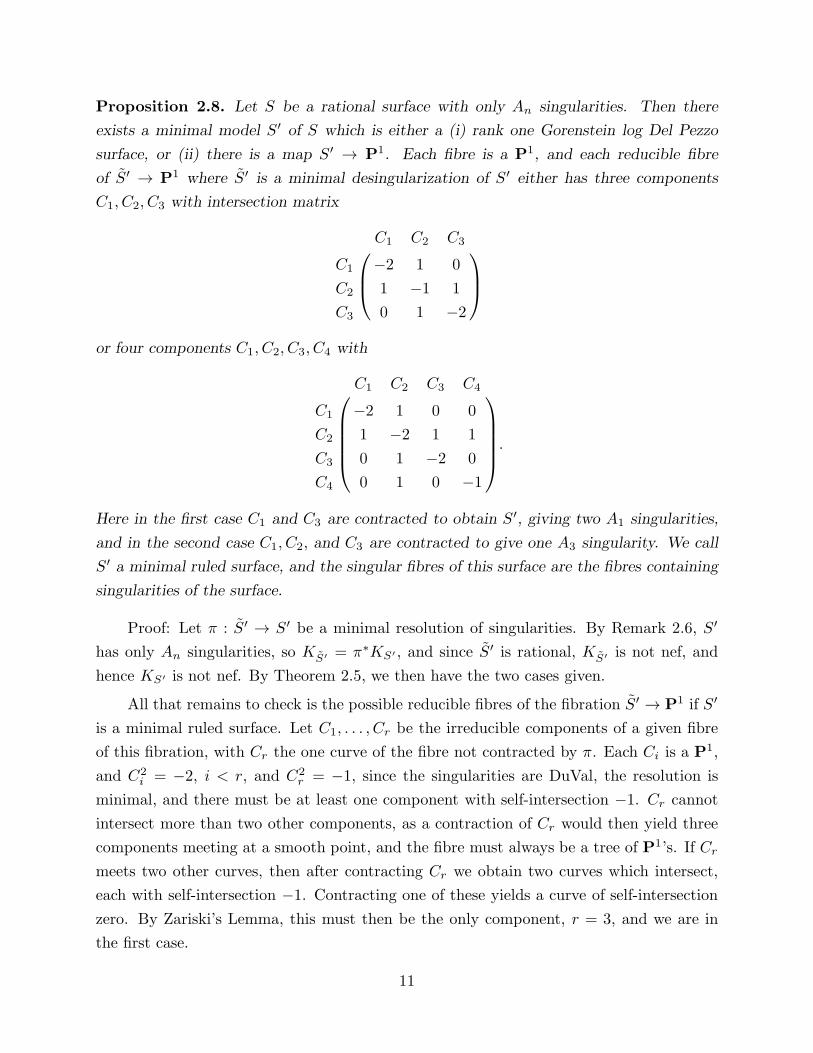
Proposition 2.8. Let S be a rational surface with only An singularities. Then there
exists a minimal model S′ of S which is either a (i) rank one Gorenstein log Del Pezzo
surface, or (ii) there is a map S′ → P1. Each fibre is a P1, and each reducible fibre
of S′ → P1 where S′ is a minimal desingularization of S′ either has three components
C1, C2, C3 with intersection matrix
C1 C2 C3
C1 −2 1 0
C2 1 −1 1
C3 0 1 −2
or four components C1, C2, C3, C4 with
C1 C2 C3 C4
C1 −2 1 0 0
C2 1 −2 1 1
C3 0 1 −2 0
C4 0 1 0 −1
.
Here in the first case C1 and C3 are contracted to obtain S′, giving two A1 singularities,
and in the second case C1, C2, and C3 are contracted to give one A3 singularity. We call
S′ a minimal ruled surface, and the singular fibres of this surface are the fibres containing
singularities of the surface.
Proof: Let π : S′ → S′ be a minimal resolution of singularities. By Remark 2.6, S′
has only An singularities, so KS′ = π∗KS′ , and since S′ is rational, KS′ is not nef, and
hence KS′ is not nef. By Theorem 2.5, we then have the two cases given.
All that remains to check is the possible reducible fibres of the fibration S′ → P1 if S′
is a minimal ruled surface. Let C1, . . . , Cr be the irreducible components of a given fibre
of this fibration, with Cr the one curve of the fibre not contracted by π. Each Ci is a P1,
and C2i = −2, i < r, and C2
r = −1, since the singularities are DuVal, the resolution is
minimal, and there must be at least one component with self-intersection −1. Cr cannot
intersect more than two other components, as a contraction of Cr would then yield three
components meeting at a smooth point, and the fibre must always be a tree of P1’s. If Cr
meets two other curves, then after contracting Cr we obtain two curves which intersect,
each with self-intersection −1. Contracting one of these yields a curve of self-intersection
zero. By Zariski’s Lemma, this must then be the only component, r = 3, and we are in
the first case.
11
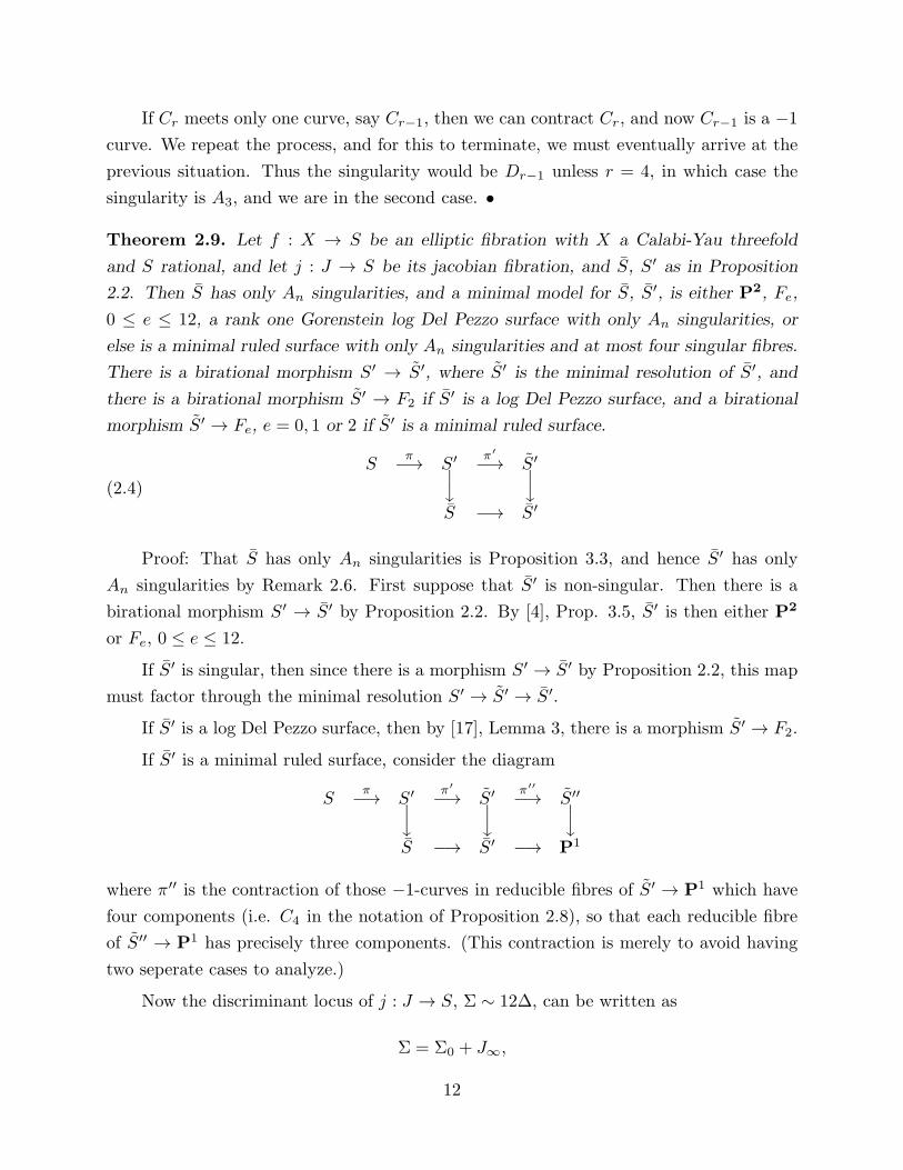
If Cr meets only one curve, say Cr−1, then we can contract Cr, and now Cr−1 is a −1
curve. We repeat the process, and for this to terminate, we must eventually arrive at the
previous situation. Thus the singularity would be Dr−1 unless r = 4, in which case the
singularity is A3, and we are in the second case. •
Theorem 2.9. Let f : X → S be an elliptic fibration with X a Calabi-Yau threefold
and S rational, and let j : J → S be its jacobian fibration, and S, S′ as in Proposition
2.2. Then S has only An singularities, and a minimal model for S, S′, is either P2, Fe,
0 ≤ e ≤ 12, a rank one Gorenstein log Del Pezzo surface with only An singularities, or
else is a minimal ruled surface with only An singularities and at most four singular fibres.
There is a birational morphism S′ → S′, where S′ is the minimal resolution of S′, and
there is a birational morphism S′ → F2 if S′ is a log Del Pezzo surface, and a birational
morphism S′ → Fe, e = 0, 1 or 2 if S′ is a minimal ruled surface.
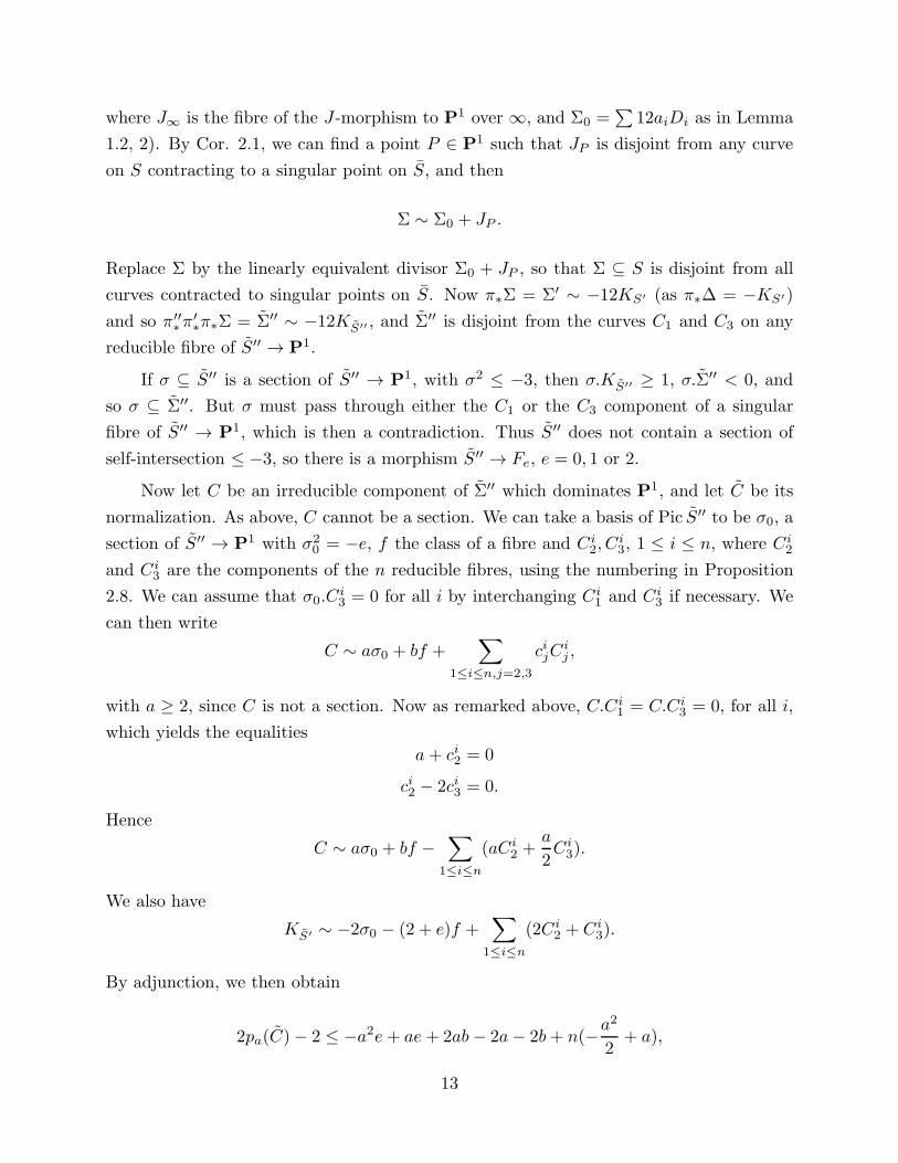
(2.4)
Sπ−→ S′ π′
−→ S′
y
y
S −→ S′
Proof: That S has only An singularities is Proposition 3.3, and hence S′ has only
An singularities by Remark 2.6. First suppose that S′ is non-singular. Then there is a
birational morphism S′ → S′ by Proposition 2.2. By [4], Prop. 3.5, S′ is then either P2
or Fe, 0 ≤ e ≤ 12.
If S′ is singular, then since there is a morphism S′ → S′ by Proposition 2.2, this map
must factor through the minimal resolution S′ → S′ → S′.
If S′ is a log Del Pezzo surface, then by [17], Lemma 3, there is a morphism S′ → F2.
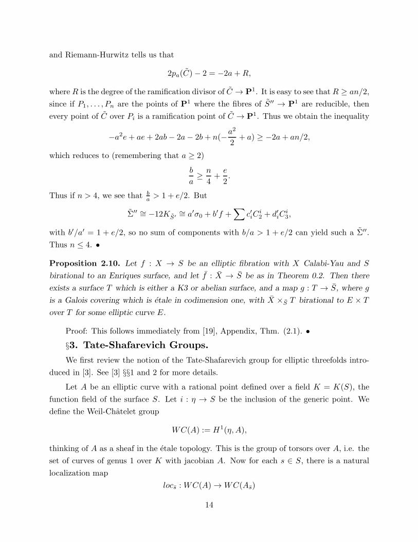
If S′ is a minimal ruled surface, consider the diagram
Sπ−→ S′ π′
−→ S′ π′′
−→ S′′
y
y
y
S −→ S′ −→ P1
where π′′ is the contraction of those −1-curves in reducible fibres of S′ → P1 which have
four components (i.e. C4 in the notation of Proposition 2.8), so that each reducible fibre
of S′′ → P1 has precisely three components. (This contraction is merely to avoid having
two seperate cases to analyze.)
Now the discriminant locus of j : J → S, Σ ∼ 12∆, can be written as
Σ = Σ0 + J∞,
12
where J∞ is the fibre of the J-morphism to P1 over ∞, and Σ0 =∑
12aiDi as in Lemma
1.2, 2). By Cor. 2.1, we can find a point P ∈ P1 such that JP is disjoint from any curve
on S contracting to a singular point on S, and then
Σ ∼ Σ0 + JP .
Replace Σ by the linearly equivalent divisor Σ0 + JP , so that Σ ⊆ S is disjoint from all
curves contracted to singular points on S. Now π∗Σ = Σ′ ∼ −12KS′ (as π∗∆ = −KS′)
and so π′′∗π
′∗π∗Σ = Σ′′ ∼ −12KS′′ , and Σ′′ is disjoint from the curves C1 and C3 on any
reducible fibre of S′′ → P1.
If σ ⊆ S′′ is a section of S′′ → P1, with σ2 ≤ −3, then σ.KS′′ ≥ 1, σ.Σ′′ < 0, and
so σ ⊆ Σ′′. But σ must pass through either the C1 or the C3 component of a singular
fibre of S′′ → P1, which is then a contradiction. Thus S′′ does not contain a section of
self-intersection ≤ −3, so there is a morphism S′′ → Fe, e = 0, 1 or 2.
Now let C be an irreducible component of Σ′′ which dominates P1, and let C be its
normalization. As above, C cannot be a section. We can take a basis of Pic S′′ to be σ0, a
section of S′′ → P1 with σ20 = −e, f the class of a fibre and Ci2, C
i3, 1 ≤ i ≤ n, where Ci2
and Ci3 are the components of the n reducible fibres, using the numbering in Proposition
2.8. We can assume that σ0.Ci3 = 0 for all i by interchanging Ci1 and Ci3 if necessary. We
can then write
C ∼ aσ0 + bf +∑
1≤i≤n,j=2,3
cijCij ,
with a ≥ 2, since C is not a section. Now as remarked above, C.Ci1 = C.Ci3 = 0, for all i,
which yields the equalities
a+ ci2 = 0
ci2 − 2ci3 = 0.
Hence
C ∼ aσ0 + bf −∑
1≤i≤n
(aCi2 +a
2Ci3).
We also have
KS′ ∼ −2σ0 − (2 + e)f +∑
1≤i≤n
(2Ci2 + Ci3).
By adjunction, we then obtain
2pa(C)− 2 ≤ −a2e+ ae+ 2ab− 2a− 2b+ n(−a2
2+ a),
13
and Riemann-Hurwitz tells us that
2pa(C)− 2 = −2a+R,
where R is the degree of the ramification divisor of C → P1. It is easy to see that R ≥ an/2,
since if P1, . . . , Pn are the points of P1 where the fibres of S′′ → P1 are reducible, then
every point of C over Pi is a ramification point of C → P1. Thus we obtain the inequality
−a2e+ ae+ 2ab− 2a− 2b+ n(−a2
2+ a) ≥ −2a+ an/2,
which reduces to (remembering that a ≥ 2)
b
a≥n
4+e
2.
Thus if n > 4, we see that ba> 1 + e/2. But
Σ′′ ∼= −12KS′
∼= a′σ0 + b′f +∑
c′iCi2 + d′iC
i3,
with b′/a′ = 1 + e/2, so no sum of components with b/a > 1 + e/2 can yield such a Σ′′.
Thus n ≤ 4. •
Proposition 2.10. Let f : X → S be an elliptic fibration with X Calabi-Yau and S
birational to an Enriques surface, and let f : X → S be as in Theorem 0.2. Then there
exists a surface T which is either a K3 or abelian surface, and a map g : T → S, where g
is a Galois covering which is etale in codimension one, with X ×S T birational to E × T
over T for some elliptic curve E.
Proof: This follows immediately from [19], Appendix, Thm. (2.1). •
§3. Tate-Shafarevich Groups.
We first review the notion of the Tate-Shafarevich group for elliptic threefolds intro-
duced in [3]. See [3] §§1 and 2 for more details.
Let A be an elliptic curve with a rational point defined over a field K = K(S), the
function field of the surface S. Let i : η → S be the inclusion of the generic point. We
define the Weil-Chatelet group
WC(A) := H1(η, A),
thinking of A as a sheaf in the etale topology. This is the group of torsors over A, i.e. the
set of curves of genus 1 over K with jacobian A. Now for each s ∈ S, there is a natural
localization map
locs :WC(A)→ WC(As)
14
where As = A×η ηs and ηs is the function field of OS,s, the strict henselization of the local
ring of S at s. The map is given by E 7→ E ×η ηs. We define the Tate-Shafarevich group
to be
XS(A) :=⋂
s∈S
ker(locs).
This turns out to be also H1(S, i∗A), with cohomology in the etale topology.
We can identify XS(A) with the set
{E ∈WC(A)|XE → S has a rational section locally in the etale topology at every point s ∈ S}
where XE → S is proper and a model of E (i.e. (XE)η = E.) Thus if E ∈ XS(A),
f : X → S a model for E, then f can have only isolated multiple fibres. In this case, if
s ∈ S and Xs is an isolated multiple fibre, f still has a rational section locally at s. Such
an isolated multiple fibre is called a locally trivial isolated multiple fibre. (See [3], 2.19.)
If f : X → S is an elliptic fibration with only locally trivial isolated multiple fibres,
with X birational to a Calabi-Yau, then we have seen in Proposition 2.2 that its jacobian,
j : J → S, is also birational to a Calabi-Yau. Thus as a first approximation to a finiteness
theorem, we would hope that XS(A) is finite where A is the generic fibre of j.
In [3], §1, we have shown how to calculate XS(A) if j : J → S is a Miranda model.
From this we obtain almost immediately the following crucial theorem. Note that this fails
for elliptic K3 surfaces, since h2(OX) 6= 0 when X is K3. This explains why our main
theorem is not true in the K3 case.
Proposition 3.1. If J → S is a Miranda fibration with generic fibre A and J a Calabi-Yau
threefold and S projective, then XS(A) is a finite group.
Proof: By [3], Theorem 2.24, XS(A) is an extension of (Q/Z)r by a finite group,
where r is the corank of XS(A), and
r = b2(J)− ρ(J)− (b2(S)− ρ(S))
where ρ is the rank of the Picard group and b2 is the second Betti number. Since h2(OJ ) =
h2(OS) = 0, b2(J) = ρ(J) and b2(S) = ρ(S). Thus r = 0 and XS(A) is a finite group. •
Of course, an elliptic Calabi-Yau threefold might have multiple fibres which are not
locally trivial. The group XS−Z(A)/XS(A) measures the additional fibrations one ob-
tains by allowing multiple fibres along Z. Since only isolated multiple fibres are allowed
on the minimal model of an elliptic Calabi-Yau threefold, we consider sets Z which can be
contracted to a set of points. This motivates the following proposition. The proof requires
familiarity with the results and notation of [7].
15
Proposition 3.2. Let j : J → S be a Miranda model with generic fibre A, and let Ei ⊆ S,
1 ≤ i ≤ n be irreducible projective curves with the intersection matrix (Ei.Ej) negative
definite. Then the group
XS−⋃
Ei(A)/XS(A)
is a finite group.
Proof: Put Z =⋃
Ei, and order the Ei’s so that E1, . . . , En1are of fibre-type I0 with
j−1(Ei) = Ei × Ci for elliptic curves Ci, 1 ≤ i ≤ n1, En1+1, . . . , En2are of fibre type Ia,
Case I, a ≥ 1. (See [7], §1, for the distinction between Case I and Case I∗ for curves
of fibre type Ia, a ≥ 1.) The remaining components of Z will be curves not of this type.
Then from [7, 2.11],
H2Z(S, i∗A) ⊆
n1⊕
i=1
MW (j−1(Ei)/Ei)tors ⊕
n2⊕
i=n1+1
Q/Z⊕G,
where G is a finite group and MW (j−1(Ei)/Ei) is the Mordell-Weil group of the elliptic
surface j−1(Ei) → Ei. Indeed, from [7], 2.11, G has various finite contributions from
curves of type Ia, Case I∗, a finite number of collisions of type I∗0 + III, and the torsion
parts of Mordell-Weil groups of non-trivial elliptic surfaces, which by the Mordell-Weil
theorem are finitely generated, and hence have finite torsion.
By the exact sequence of local cohomology, we have
XS−Z(A)/XS(A) ∼= ker(H2Z(S, i∗A)
φ−→H2(S, i∗A)).
So, while H2Z(S, i∗A) may well be infinite, we can show that the kernel of φ is finite. Recall
from [7] that if γ ∈ H2Z(S, i∗A), then φ(γ) = 0 if and only if the so-called first and second
obstructions of γ are zero. See [7], §4, for details.
Let γ1, . . . , γn2be the invariants of an element γ of H2
Z(S, i∗A) along the curves
E1, . . . , En2, with γ1, . . . , γn1
∈ (Q/Z)⊕2 = MW (j−1(Ei)/Ei)tors and γn1+1, . . . , γn2∈
Q/Z. (See [7], Remark 2.12) Consider the first obstruction along the curves En1+1, . . . , En2.
By [7] Theorems 4.5 and 4.3, this obstruction being zero requires in particular that for all
l
(3.1)
(
n2∑
i=n1+1
γiEi.El
)
+ kl = 0,
where kl ∈ Q/Z depends on the other invariants of γ along the curves Ei, i > n2. These
invariants take values in the finite group G, and thus kl can only take on a finite number
16
of possible values. Now the intersection matrix (Ei.El)n1+1≤i,l≤n2is negative definite, and
as a result, the number of solutions to (3.1) is finite for any given set of values for the kl’s.
Thus there are only a finite number of possibilities for the γi, n1 + 1 ≤ i ≤ n2.
A similar argument works for the γi, 1 ≤ i ≤ n1, but we need to use the second
obstruction, which is a codimension 2 algebraic cycle on J . Identifying (PicCi)tors with
(Q/Z)⊕2, following [7], Examples 5.2, 1) and 2), we obtain a cycle of the following form.
If πi : Ei ×Ci → Ci is the second projection, fi : Ei ×Ci → J the inclusion, ci ∈ (Ci)tors,
then the second obstruction is a cycle
α =
(
n∑
i=1
fi∗π∗i (γi)
)
+ β,
where β is a cycle which again only takes on a finite number of possible different values.
In order to realise this set of invariants, we need α to be rationally equivalent to zero. In
order for this to be possible, in particular we must have πl∗f∗l (α) linearly equivalent to
zero on each curve Cl, i.e.
(3.2) πl∗f∗l (α) =
(
n∑
i=1
γiEi.El
)
+ kl = 0,
as an equation in (Q/Z)⊕2, where the kl come from the cycle β and thus take on only a
finite number of possible values. We then argue as before, and the γi, 1 ≤ i ≤ n, take on
only a finite number of values. •
As an application of the above proof, we obtain
Proposition 3.3. The singularities occuring in S in Theorem 0.2 are all An singularities,
i.e the minimal resolution consists of a chain of −2 curves.
Proof: As usual, we have f : X → S, j : J → S as given in Lemmas 1.2 and 1.6. We
have the resolution S → S of the singularities of S. Let P ∈ S be a singular point. Then
φ−1(P ) consists of curves E1, . . . , Er which are all isomorphic to P1. By Corollary 2.1,
there are two cases. Either j−1(Ei) = Ei×Ci for an elliptic curve Ci, or all Ei are of fibre
type Ia, a ≥ 1 and Case I. Thus either formulae (3.1) or (3.2) are relevant, except that
there is no kl. Thus we obtain, with γ1, . . . , γr ∈ (Q/Z)⊕2 or Q/Z depending on the two
cases, the following system of equations in (Q/Z)⊕2 or Q/Z:
r∑
i=1
γiEi.El = 0, 1 ≤ l ≤ r.
17
The multiplicity of the fibres over Ei in the fibration f : X → S, mi, is the order of γi
([7], 2.12).
Now in the notation of the proof of Theorem 0.2, ai = b′i = 0 for all i. Thus by (2.3),
if di = 0 for some i, then we must have mi > 0, and hence γi 6= 0. Let C = (Ei.Ej) be
the intersection matrix of the Ei’s. Then γi = 0 if the ith row of C−1 consists of integers.
If the resolution is minimal, it is easy to check that there exists integral rows in C−1 for
singularities Dm or Em. (In fact, for E8, C−1 itself is integral). If the resolution is not
minimal, then it is a blowup of a minimal resolution, and it is easy to see that blowing up
does not effect the integrality of a row in C−1. •
Example 3.4. Let f1 : Y1 → P1 and f2 : Y2 → P1 be two rational elliptic surfaces,
with Y1 → P1 having two singular fibres of type I∗0 . Such a surface exists by [16], Theorem
4.1. Let X = Y1×P1 Y2 with p1, p2 : X → Y1, Y2 the projections. If Y2 is chosen so that no
singular fibres of f1 and f2 map to the same point in P1, then X is a non-singular Calabi-
Yau threefold, and p1 and p2 are elliptic fibrations. (See [23], §2) Let P ∈ P1 be a point
with the fibre (Y1)P of type I∗0 and (Y2)P = E ⊆ Y2 a non-singular elliptic curve. (Y1)P
has five components C1, . . . , C5 with C5 having multiplicity 2. We have p−11 (Ci) ∼= Ci×E.
We wish to perform a logarithmic transformation along C1, . . . , C4.
Let P1, P0 ∈ E ⊆ Y2 be two points with P1 − P0 a 2-torsion element in PicE, and
consider the cycle on X given by p∗2(P1 − P0). Since Y2 is rational, P1 − P0 is rationally
equivalent to zero on Y2, so p∗2(P1 − P0) ∼ 0 on X . Now
p∗2(P1 − P0) =
4∑
i=1
αi∗(P1 × Ci − P0 × Ci) + 2α5∗(P1 × C5 − P0 × C5)
∼4∑
i=1
αi∗(P1 × Ci − P0 × Ci)
where αi : Ci×E → X is the inclusion. (The last rational equivalence is because P1−P0 is
2-torsion in E.) Because this expression is rationally equivalent to zero, as in [7], Example
5.2. we can then obtain a threefold X ′ → Y1 whose jacobian is p1 : X → Y1 with fibres
of multiplicity 2 along C1, . . . , C4. X′ is not minimal, but as in the proof of Theorem 0.2,
one can contract C1, . . . , C4 to obtain a surface Y1 and a minimal Calabi-Yau threefold X ′
with a fibration X ′ → Y1. Y1 has four A1 points.
We now put results of the last section and this section together. This statement is
very close to our final result; we will only need to show how Ogg-Shafarevich theory works
in families, which we will do in the next section.
18
Proposition 3.5. Let f : X → S be a Calabi-Yau elliptic fibration with S rational and
generic fibre E and Jac(E) = A. Let S′ and S′ be as in Theorem 2.9. Then there exists
sections a ∈ Γ(S′, ω−4
S′) and b ∈ Γ(S′, ω−6
S′) such that the Weierstrass model
W (ω−1
S′, a, b)→ S′
is minimal and has generic fibre A. If Σred is the reduced discriminant locus of this
Weierstrass model, let Z ⊆ S′ be the union of sing(Σred) and the exceptional locus of
S′ → S′. Then E ∈XS′−Z(A). Furthermore, this latter group is finite.
Proof. As in Proposition 2.2, we have a jacobian fibration j′ : J ′ → S′ with KJ ′ = 0.
We obtained a composed fibration J ′ → S′. This fibration has a rational section, and
hence we can find a birationally equivalent minimal Weierstrass fibration
w : W :=W (L, a, b)→ S′.
It is then easy to see that L ∼= ω−1
S′. Indeed, KW = w∗(ωS′⊗L), and if T = S′−sing(Σred),
WT = W ×S′ T has a canonical crepant resolution of singularities φ : WT → WT with
KWT= φ∗KWT
. Furthermore, WT → T and J ′T = J ′×S′T → T are birationally equivalent
and both are relatively minimal; since KJ ′
T= 0, this implies that KWT
= 0 also, and hence
KWT= KW = 0. Thus L ∼= ω−1
S′.
Now consider the fibration X → S′. Σm for this fibration consists of a finite number
of points, as Σm for X → S consists of isolated points. Every one of these points must
be either at a singular point of S′ or a singular point of the reduced discriminant locus of
X → S, Σred, by [3], Cor. 3.2. Let Z ′ = sing(Σred) ∪ sing(S′). Then S′ − Z ′ = S′ − Z,
and clearly E ∈XS′−Z′(A) = XS′−Z(A).
Finally, to show the finiteness statement, let JM → M be a Miranda model for A
obtained by blowing up S′. The exceptional locus of ψ : M → S′ maps to Z, since we
only need to blow-up points of sing(Σred). Now ψ−1(Z) consists of a finite number of
points and a union E1 ∪ · · · ∪En of P1’s whose intersection matrix is negative definite by
Grauert’s criterion. Now Proposition 3.1 tells us that XM (A) is finite, Proposition 3.2
tells us that XM−E1∪···∪En(A) is then finite, and [3], Cor. 3.2 tells us that removing a
finite number of further points can only increase the Tate-Shafarevich group by a finite
group, so that XM−ψ−1(Z)(A) = XS′−Z(A) is a finite group.
§4. Proof of the Main Theorem.
19
Definition 4.1. A family of elliptic three-folds is a triple (X ,S, T ) of non-singular quasi-
projective varieties with a diagram
X
yf
π
ց
Sg−→ T
with f, g and π projective, g and π smooth of relative dimension 2 and 3 respectively, and
the generic fibre of f a geometrically regular curve of genus 1.
Lemma 4.2. Let g : S → T be a family of smooth projective surfaces, L a line bundle
on S. Then there exists a finite number of families (Xi,Si, Ti) of elliptic fibrations with
fi : Xi → Si having a section, along with Xi → Wi(Li, ai, bi) a resolution of singularities
of a Weierstrass model over Si, and also with Cartesian diagrams
Si −→ Ti
y
αi
y
S −→ T
with Li ∼= α∗iL, such that the following property holds. For any t ∈ T , S = St, a ∈
Γ(S,L⊗4|S), b ∈ Γ(S,L⊗6|S) with 4a3 + 27b2 6= 0, there exists a t′ ∈ Ti for some i with
ai|(Si)t′= a, bi|(Si)t′
= b. Furthermore, we can assume that fi : Xi → Si is flat away from
the singularities of the reduced discriminant locus of fi.
Proof: Let E = L⊗4 ⊕ L⊗6, and let T ′ = V((g∗E)∨) and S′ = V((g∗g∗E)
∨), where
V(F) = Spec(S(F)), S(F) the symmetric algebra of F . By semicontinuity, we can split
T up into a finite number of locally closed subsets of T on which g∗E is locally free, so we
can assume that g∗E is indeed locally free. We have a diagram
S′π′
−→ S
yg′
y
g
T ′ π−→ T
Now π′∗E has a universal section given by the composition
OS′ → π′∗g∗g∗E → π′∗E
where the first map is the universal section of π′∗g∗g∗E ([9], 9.4.9). If we write this section
as (a, b), a ∈ Γ(S′, π′∗L⊗4) and b ∈ Γ(S′, π′∗L⊗6), then if t′ ∈ T ′ corresponds to a point
(t, a′, b′), t ∈ T , a′ ∈ Γ(St,L⊗4|St
), b′ ∈ Γ(St,L⊗6|St
), then a, b|(S′)t′= a′, b′. We then
have a universal Weierstrass model
W ′ = W (π′∗L, a, b)→ S′,
20
and we can replace T ′ with the open subset
{t′ ∈ T ′|4a3 + 27b2 is not identically zero on (S′)t′},
and replace S′ with the inverse image of this open subset. Thus we can assume that no
fibre of g′ is contained in the discriminant locus Σ ⊆ S′.
Now let X ′ →W ′ be a resolution of singularities, and let T1 ⊆ T′ be a dense open set
on which X ′ → T ′ is smooth, S1 = S′ ×T ′ T1, X1 = X ′ ×T ′ T1, and
W1 = W (π′∗L|S1, a|S1
, b|S1)→ S1.
As in [15], §7, this resolution can be performed canonically away from the singular points
of the reduced discriminant locus Σred of W ′ → S′. Thus we can assume that X ′ → S′ is
flat away from sing(Σred). Note also that a Weierstrass model is always non-singular at
the section at infinity, so the resolution can be performed so that X ′ → S′ has a section.
Now replace T ′ with a finite disjoint union of non-singular locally closed subsets of T ′−T1,
whose union is T ′ − T1, replace W′ and S′ with restrictions of these to the new T ′, and
then construct a resolution of singularities of the smaller W ′. By Noetherian induction,
we eventually cover all of T ′ in this fashion, proving the theorem. •
Theorem 4.3. Let (X , S, T ) be a family of elliptic fibrations such that f : X → S has
a section, and let S ⊆ S be an open subset, X = S ×S X . Assume furthermore that the
reduced discriminant locus Σred of f : X → S is smooth over T , every component of Σred
surjects onto T , and that f is flat. Furthermore, assume that for all t ∈ T , XSt(At) is a
finite group, where At is the generic fibre of Xt → St. Then there exists a finite collection
of families of elliptic threefolds (Xi, Si, Ti) with maps pi : Ti → T and Si = Ti ×T S, such
that for all t ∈ T , and for all Et ∈ XSt(At), there exists a t′ ∈ Ti for some i such that
(Xi)t′ → (Si)t′ has generic fibre Et.
We will need five lemmas:
Lemma 4.4. Let i : η → S be the inclusion of the generic point of S into S in the
situation of Theorem 4.3, g : S → T the restriction of g : S → T . Then for any integer
n > 0, nR1g∗(i∗A), the n-torsion subsheaf of R1g∗(i∗A), is a constructible sheaf on T ,
where A is the generic fibre of f : X → S.
Proof: Let Σ be the discriminant locus of the elliptic fibration f : X → S. Then
R1g∗(i∗A) ⊆ R1g′∗(i∗A)|S−Σ,
21
where g′ is the restriction of g to S − Σ. This can be verified on stalks since XS(A) ⊆
XU (A) whenever U ⊆ S is an open subset of a variety S. Since a subsheaf of a constructible
sheaf is constructible ([14, V 1.9]), it is enough to show the Lemma when Σ is empty,
replacing S by S − Σ. Assume that Σ is empty. By [3], 1.11 and 1.12, we have
PX/S∼= i∗i
∗PX/S
where PX/S = R1f∗Gm for a morphism f : X → S, and we also have the exact sequence
0→ i∗A→ i∗i∗PX/S → Z→ 0.
([3], §1, (6)) Applying g∗, we see that
R1g∗(i∗A) ∼= R1g∗(i∗i∗PX/S) ∼= R1g∗PX/S .
Now by the Leray spectral sequence and [3], 1.4, we have
R1g∗PX/S∼=R2π∗Gm
R2g∗Gm,
where π : X → T is the restriction of π : X → T . Taking n-torsion, we see that we obtain
an exact sequence
0→ nR2g∗Gm → nR
2π∗Gm → nR1g∗PX/S → (R2g∗Gm)⊗Z/nZ
φ−→(R2π∗Gm)⊗ Z/nZ,
and by the Kummer sequence we obtain a diagram
0 −→ (R2g∗Gm)⊗ Z/nZ −→ R3g∗µn
yφ
yf∗
0 −→ (R2π∗Gm)⊗ Z/nZ −→ R3π∗µn
Since f∗ is injective as f has a section, φ is also injective, and hence we obtain
nR1g∗PX/S
∼=nR
2π∗Gm
nR2g∗Gm.
Now we have by the Kummer sequence that R2π∗µn → nR2π∗Gm → 0, and R2π∗µn is
constructible, so (R2π∗Gm)n is also. Tracing back, we obtain the Lemma. •
Let f : X → Y be a smooth, proper morphism, and let D ⊆ X be an effective divisor,
D = D1 ∪ · · · ∪Dn, with the Di irreducible components of D. We say D is simple normal
crossings relative to Y if whenever x ∈ D, and I = {i|x ∈ Di}, then⋂
i∈I Di → Y is
smooth of relative dimension dimX − dimY −#I.
22
Lemma 4.5. Let f : X → Y be a proper, smooth morphism with X and Y of finite
type over a field of characteristic zero. Let D ⊆ X be a divisor which has simple normal
crossings over Y . Let F be a locally constant constructible torsion sheaf on X , and let
g : X − D → Y be the restriction. Then Rig∗F commutes with arbitrary base changes
over Y .
Proof. This is a standard application of purity (see e.g. [2], Th. Finitude, Appendice).
First note that the lemma is true if D is empty by the proper base change theorem
([14], VI 2.3). Now let
Xr = X −⋃
#I=r
(
⋂
i∈I
Di
)
,
and Xn+1 = X , where n is the number of components of D. We then have a diagram
Xr−1 → Xri←− Xr −Xr−1 = Zr
g
ց
yf
h
ւ
S
Since D is simple normal crossings over Y , h is smooth.
By [14], VI 5.3, there is an exact sequence
· · · → Rj−2c−1h∗(i∗F ⊗ TZr/Xr
)→ Rj−1f∗(F|Xr)→ Rj−1g∗(F|Xr−1
)
→ Rj−2ch∗(i∗F ⊗ TZr/Xr
)→ Rjf∗(F|Xr)→ · · ·
where TZr/Xris a locally constant sheaf on Zr. From this we see that if Rjg∗(F|Xr
) and
Rjh∗(i∗F ⊗ TZr/Xr
) commute with base change for all j, then so does Rj−1g∗(F|Xr−1).
Thus by induction on dimX and descending induction on r, we obtain the desired result.
•
Lemma 4.6. Let f : X → Y be a compactifiable smooth morphism, X and Y of finite
type over an algebraically closed field of characteristic zero. Then there exists a dense
open set U ⊆ Y such that for any locally constant constructible torsion sheaf F on X ,
(Rif∗F)y = Hi(Xy,F) for all y ∈ U , and (Rif∗F)|U is locally constant.
Proof. Let X ⊆ Xf−→Y be a compactification of f . By resolution of singularities, we
can assume that X−X is a simple normal crossings divisor. By generic smoothness, there
exists U ⊆ Y such that X −X is simple normal crossings over U . We then apply Lemma
4.5. The two claims then follow as in [14] VI 2.5 and 4.2. •
Now consider the following situation. Let f : X → S be an elliptic fibration with a
section with generic fibre A, and let S′ ⊆ S be an irreducible locally closed subset such
23
that the generic fibre A′ of f ′ : X ×S S′ → S′ is an elliptic curve. Let i be the inclusion
of the generic point of S in S and i′ the inclusion of the generic point of S′ in S′. Let
g : S′ → S be the inclusion. I claim there is a natural restriction map
XS(A)→XS′(A′)
defined as follows. First, there is a map
i∗A→ g∗i′∗A
′.
Indeed, a section of i∗A corresponds to a rational section of f over an open set U . By
restricting this rational section to U ′ = U ×S S′, we obtain a rational section of f ′ over
U ′ provided that the original section was defined over an open dense set of S′. But this is
indeed the case, as a rational section is always defined where f is smooth by [20], Lemma
1.9. Thus we obtain a composition H1(S, i∗A)→ H1(S, g∗i′∗A
′)→ H1(S′, i∗A′), the latter
map by the Leray spectral sequence. This is the desired restriction map. It is then clear
that if E ∈XS(A) and g : Y → S is an elliptic fibration with generic fibre E, and if g|S′
is an elliptic fibration over S′, then the latter has generic fibre E|S′, the image of E in
XS′(A′).
As one particular case of this, there is, in our situation in Theorem 4.3, a restriction
map
(R1g∗(i∗A))t →XSt(At)
where At is the generic fibre of Xt → St whenever t ∈ T is a closed point. Indeed,
(R1g∗(i∗A))t ∼= H1(S ×T SpecOT ,t, i∗A) where OT ,t is the strict henselization of the local
ring of T at t, and we then use the above restriction map with S′ = St. We then have
Lemma 4.7. In the situation of Theorem 4.3, there exists a dense Zariski open subset
U ⊆ T for which the following is true. For all closed points t ∈ U , with At the generic
fibre of Xt → St, the natural restriction map
(nR1g∗(i∗A))t → nXSt
(At)
is surjective, for any integer n.
Proof: First, let Σ be the discriminant locus of f . Let g′ : S′ = S − Σ → T be the
restriction of g, X ′ = S′ ×S X , and f′, π′ the restrictions of f and π to X ′. As shown in
the proof of Lemma 4.4, we have
nR1g′∗(i∗A)|S′
∼=nR
2π′∗Gm
nR2g′∗Gm
24
and similarly
nXS′
t(At) =
nH2(X ′
t ,Gm)
nH2(S′t,Gm).
To show the lemma for S′, it is then enough to show that there is some open set U ⊆ T
such that the natural restriction map
n(R2π′
∗Gm)t → nH2(X ′
t ,Gm)
is surjective for t ∈ U for any n. But by the Kummer sequence, we have a diagram
(R2π′∗µn)t −→ n(R
2π′∗Gm)t −→ 0
y
y
H2(X ′t , µn) −→ nH
2(X ′t ,Gm) −→ 0
By Lemma 4.5, the first vertical arrow is surjective for all n for t ∈ U for some dense open
set U of T , and hence so is the second. This proves the Lemma for the family (X ′,S′, T ).
Now note that
(R1g′∗(i∗A)|S′)t = XS′(t)(A(t))
where S′(t) = S′ ×T SpecOT ,t, and A(t) = A ×η η(t), where η(t) is the generic point of
S′(t). We have a similar equality for g, and hence a diagram
0 −→ nXS(t)(A(t)) −→ nXS′(t)(A(t))
y
r1
y
r2
0 −→ nXSt(At) −→ nXS′
t(At)
We have shown that r2 is surjective for t ∈ U . We wish to show that r1 is.
Let E ∈ nXSt(At), E
′ ∈ nXS′(t)(A(t)) with r2(E′) = E. Let Z ⊆ S(t) be the closed
subset of S(t) defined by
Z = {s ∈ S(t)|locs(E′) 6= 0}.
Suppose Z 6= φ. Let s1, . . . , sn be the generic points of the irreducible components of Z.
Since Σ → T is smooth, Σ ×T SpecOT ,t in particular is non-singular, and hence by [3],
Cor. 3.2, all the si are generic points of Σ ×T SpecOT ,t. Thus {si} ∩ St 6= φ (as each
component of Σ surjects onto T ), and if s′i is the generic point of this intersection, then
locs′i(E) 6= 0, contradicting E ∈XSt
(At). Thus Z = φ and E′ ∈XS(t)(A(t)) and r1 is
surjective. •
25
Lemma 4.8. With the hypothesis of Theorem 4.3, there exists an n ∈ Z and a dense
open subset U ⊆ T such that XSt(At) is killed by n for all closed points t ∈ U .
Proof: First we claim that there exists a dense open set U ⊆ T for which
H2(Xt,Gm)/H2(St,Gm)
is constant for all t ∈ U , assuming that it is always finite. Recall from [8], II 3.2 that if X
is a scheme smooth over a field k of characteristic zero, then H2(X,Gm) = (Q/Z)r⊕G for
some finite group G and some r. We define H2(X,Gm)f := G. Thus since we are assuming
H2(Xt,Gm)/H2(St,Gm) is finite, this group is the same as H2(Xt,Gm)f/H2(St,Gm)
f .
Furthermore, H2(X,Gm)f (l) = H3(X,Zl[1])tors by [8], III, (8.9). Thus by Lemma 4.5,
there exists an open subset U ⊆ T such that these groups are constant.
Now from the proof of [3], Theorem 2.24 a), there exists a locally constant sheaf G on
the discriminant locus Σ of f which is represented by an etale scheme over Σ such that
there is an exact sequence
0→ H2(Xt,Gm)/H2(St,Gm)→XSt
(At)→ H1(Σt,G|St)
for all closed points t ∈ T . Again by Lemma 4.5, there is an open subset U ⊆ T on which
the latter group is constant (and finite). This proves the Lemma. •
Proof of Theorem 4.3: We prove the theorem by Noetherian induction, proving it for
a dense open subset U ⊆ T . By [14, V, 1.8], there exists an open subset U ⊆ T for which
F = nR1g∗(i∗A)|U is locally constant with finite stalks, (with n given by Lemma 4.8), as
the latter sheaf is constructible by Lemma 4.4. Thus there exists an etale cover U ′ → U
with F|U ′ constant, F|U ′∼= GU ′ , G a finite group. Now for all x ∈ U ′, g ∈ G, there exists
an etale neighborhood Ux,g → U ′ of x such that the element of the stalk g ∈ (F|U ′)x = G
is represented by an element Ex,g ∈ H1(Ux,g ×T S, i∗A). By quasi-compactness, we can
find an open subcover of {Ux,g|x ∈ U ′} which covers U ′, for each g. In this manner,
one obtains a finite collection of connected etale schemes U1, . . . , Un over U ′ and elements
Ej ∈ H1(Uj×T S, i∗A) such that for all closed points t ∈ U , restricting each Ej to St gives
all elements of XSt(At), by Lemmas 4.7 and 4.8.
We now only have to construct suitable models for the Ei. We will find a decompo-
sition of Ui into a finite number of locally closed subsets Tij along with families of elliptic
fibrations (Xij , Sij , Tij), Sij ∼= Tij ×T S, such that the generic fibre of Xij → Sij is Ei|Sij.
This can be done by constructing a family (Xi1,Si1, Ti1) with Ti1 ⊆ Ui a dense open subset,
and then applying Noetherian induction, replacing Ui with a finite number of non-singular
26
locally closed subsets of Ui whose union is the complement of Ti1 in Ui, and then restricting
Ei to the inverse image of these locally closed subsets on Si = S ×T Ui.
One can construct a projective morphism fi : Xi → Si, where Si = S ×T Ui, with
generic fibre Ei, and by resolution of singularities, Xi can be taken to be non-singular.
Now there is an open set Ti1 ⊆ Ui on which Xi → Ui is smooth, by generic smoothness.
This gives the desired family. •
Proof of Theorem 0.1: First apply Theorem 4.2 to a number of different families, with
L = ω−1S/T :
1) T a point, S a P2 or Fe, 0 ≤ e ≤ 12.
2) Si → Ti a finite set of families of surfaces which are minimal resolutions of all possible
rank one Gorenstein log Del Pezzo surfaces with only An singularities.
3) Si → Ti a finite set of families which include all possible surfaces S of the following
type: S is a minimal resolution of a minimal ruled surface S′ → P1 with ≤ 4 singular
fibres with only An singularities, and there is a birational morphism S → Fe, 0 ≤ e ≤
2.
It is not hard to construct the families in 2) and 3): in case 2), any minimal resolution
of a Gorenstein log Del Pezzo surface is the blowup of F2 in ≤ 7 points, by [17], Lemma
3. In this case, there is a map Si → S′i over Ti induced by some sufficiently high power
of L which contracts only the −2 curves on the fibres of Si → Ti. Let Ei ⊆ Si be the
exceptional locus of this contraction.
In case 3), any such surface is a blowup of Fe, 0 ≤ e ≤ 2, in ≤ 12 points. For example,
to construct a family of resolutions which map to Fe of minimal ruled surfaces with two
A1 singularities and one singular fibre, put T = Fe, and obtain S by first blowing up
Fe × T along the diagonal ∆ to obtain α : S′ → Fe × T with exceptional locus ∆. Let
p : Fe × T → P1 ×T be the natural ruling. Next blow up S′ along ∆ ∩ F , where F is the
proper transform of p−1(p(∆)) via α. This new blow-up is S. Let E ⊆ S be the union of
the proper transforms of ∆ and F on S. This is the union of the −2 curves on the fibres
of S → T which must be contracted to obtain the singular, minimal ruled surfaces with
one singular fibre with two A1 singularities. Likewise, one can construct other families
Si → Ti covering all such minimal ruled surfaces, and let Ei be the corresponding union of
−2 curves.
After applying Theorem 4.2, we obtain a new set of families (Xi, Si, Ti) in which in
particular any jacobian Calabi-Yau elliptic fibration appears. (We can throw out any family
which contains threefolds which aren’t Calabi-Yau which may have popped up, as being
27
Calabi-Yau is deformation invariant.) One also has Weierstrass models wi : Wi → Si. Let
Σi ⊆ Si be the reduced discriminant locus of Wi. By decomposing Ti into a finite number
of locally closed subsets, we can assume that if Zi ⊆ Σi is the locus of points where Σi → Ti
is not smooth, then each irreducible component of Σi − Zi maps surjectively to Ti. (For
this to be the case, Zi must be of relative dimension zero.) Furthermore, in cases 2) and 3)
above, we have Ei ⊆ Si which are as above. Now apply Theorem 4.3 with Si = Si−Zi∪Ei.
By Theorem 3.5, the finiteness hypothesis of Theorem 4.3 is satisfied, and Theorem 3.5
also tells us that all Calabi-Yau elliptic fibrations are thus obtained in applying Theorem
4.3. •
Bibliography
[1] Deligne, P., “Courbes Elliptiques: Formulaire d’apres J. Tate,” in Modular Functions
in One Variable IV, Lecture Notes in Mathematics vol. 476, Springer-Verlag, 1975,
pg. 53-74.
[2] Deligne, P., with Boutot, J.-F., Illusie, L., and Verdier, J.-L., SGA 4 12 , Cohomologie
Etale, Lecture Notes in Math., 569, Springer, Heidelberg 1977.
[3] Dolgachev, I., and Gross, M., “Elliptic Three-folds I: Ogg-Shafarevich Theory,” preprint,
1992 (revised version, April 1993).
[4] Grassi, A., “On Minimal Models of Elliptic Threefolds,” Math. Ann. 290, 287–301
(1991).
[5] Grassi, A., “The Singularities of the Parameter Surface of a Minimal Elliptic Three-
fold,” To appear in Int. J. of Math., 4, ???–??? (1993).
[6] Grassi, A., “Log Contractions and Equidimensional Models of Elliptic Threefolds,”
Preprint (1993).
[7] Gross, M., “Elliptic Three-folds II: Multiple Fibres,” MSRI preprint #018-93, 1992.
[8] Grothendieck, A., “Le Groupe de Brauer, I, II, III,” In Dix Exposes sur la Cohomologie
des Schemas, North-Holland, Amsterdam, 1968, 46-188.
[9] Grothendieck, A., and Dieudonne, J., Elements de Geometrie Algebrique, I,Grundlehren
der Math. Wissenschaften, 166, Springer-Verlag, (1971).
[10] Hunt, B., “A Bound on the Euler Number for Certain Calabi-Yau Threefolds,” J.
Reine Angew. Math., 411 , 137–170 (1990).
[11] Kawamata, Y., “Kodaira Dimensions of Certain Algebraic Fiber Spaces,” J. Fac. Sci.,
Tokyo Univ. IA, 30, 1–24 (1983).
[12] Kollar, J., and Mori, S., “Classification of Three-dimensional Flips,” J. of the AMS,
28
5, 533–703 (1992).
[13] Kollar, J., et al, Flips and Abundance for Algebraic Threefolds, to appear.
[14] Milne, J. Etale Cohomology, Princeton Univ. Press, 1980.
[15] Miranda, R., “Smooth Models for Elliptic Threefolds,” in Birational Geometry of
Degenerations, Birkhauser, (1983) 85-133.
[16] Miranda, R., and Persson, U., “On Extremal Rational Elliptic Surfaces,” Math. Z.,
193 537–558 (1986).
[17] Miyanishi, M., and Zhang, D.Q., “Gorenstein log Del Pezzo Surfaces of Rank One,”
Journal of Algebra, 118, 63–84, (1988).
[18] Mumford, D., and Suominen, K., “Introduction to the Theory of Moduli,” in Algebraic
Geometry, Oslo 1970, Wolters-Noordhoff Press, (1972) 171-222.
[19] Nakayama, N., “On Weierstrass Models,” Algebraic Geometry and Commutative Al-
gebra in Honor of Masayoshi Nagata, 405–431, (1987).
[20] Nakayama, N., “Local Structure of an Elliptic Fibration,” Preprint, 1991, Univ. of
Tokyo.
[21] Oguiso, K., “On Algebraic Fiber Space Structures on a Calabi-Yau Threefold,” preprint,
1992.
[22] Sakai, F., “The Structure of Normal Surfaces,” Duke Math. J., 52, 627–648 (1985).
[23] Schoen, C., “On Fiber Products of Rational Elliptic Surfaces with Section,” Math.
Z., 197, 177–199 (1988).
29